Universal time scalings of sensitivity in Markovian quantum metrology

Abstract

Assuming a Markovian time evolution of a quantum sensing system, we provide a general characterization of the optimal sensitivity scalings with time, under the most general quantum control protocols. We allow the estimated parameter to influence both the Hamiltonian as well as the dissipative part of the quantum master equation. We focus on the asymptotic-time as well as the short-time sensitivity scalings, and investigate the relevant time scales on which the transition between the two regimes appears. This allows us to characterize, via simple algebraic conditions (in terms of the Hamiltonian, the jump operators as well as their parameter derivatives), the four classes of metrological models that represent: quadratic-linear, quadratic-quadratic, linear-linear and linear-quadratic time scalings. We also provide universal numerical methods to obtain quantitative bounds on sensitivity that are the tightest that exist in the literature.

Introduction.

With rapid technological advancements, the need for precise characterizations of physical systems is getting increasingly demanding. Quantum metrology [1, 2, 3, 4, 5, 6], based on the theoretical framework of quantum estimation theory [7, 8] is a pursuit towards this goal. Understanding fundamental limits to the measurement precision arising from the basic principles of quantum mechanics and simultaneously using the quantum resources [9] like coherence [10] and entanglement [11] to achieve the optimal enhancement over classical strategies is crucial for further development of already spectacular achievements in gravitational wave detection [12, 13, 14], spectroscopy [15, 16, 17, 18, 19], magnetometry [20, 21, 22] or atomic clocks [23, 24, 25, 26, 27] to name a few.

One of the pivotal moments in the development of the field, was a realization that the potential quadratic gain in the scaling of precision with the number of resources used (particles, time), referred to as the Heiseneberg scaling [28, 16, 29, 30, 31], is extremely fragile in the presence of noise [17, 32, 33, 34, 35, 36, 37, 38, 39, 40, 41]. In commonly encountered noisy scenarios, one may asymptotically expect at most a constant quantum enhancement factor, even if all possible adaptive quantum strategies, e.g. quantum error correction protocols, are allowed [40, 41, 42, 43, 44, 45]. Nevertheless, there are also cases, when noise may be efficiently countered via quantum-error correction inspired protocols and long-time or large-scale benefits of quantum coherence/entanglement may be exploited [46, 47, 48, 49, 50, 44, 44, 45].

Figure 1: A general model of Markovian quantum sensing. A Quantum probe may be entangled with arbitrary large ancillary systems and fast and strong quantum controls can be applied during the whole sensing process. The character of the Markovian dynamics determines the optimal quantum Fisher information scaling both in the short-time as well as in the asymptotic-time regimes. The scaling may be either linear or quadratic in both regimes, and all four combinations are allowed.

In this paper, we consider the most general Markovian quantum sensing model, where the dynamics of the sensing probe is governed by the celebrated Gorini-Kossakowski-Sudarshan-Lindblad (GKSL) [51, 52] equation:

$$\frac{d\rho(t)}{dt}=\mathcal{L}_{\varphi}[\rho(t)]=-i[H(\varphi),\rho(t)]+\\ \sum_{k=1}^{n}\left(L_{k}(\varphi)\rho(t)L_{k}^{\dagger}(\varphi)-\frac{1}{2}\{L_{k}^{\dagger}(\varphi)L_{k}(\varphi),\rho(t)\}\right),$$ (1)

where the parameter $\varphi$ to be estimated may be encoded both in the Hamiltonian as well as in the jump operators $L_{k}$ that represent the noisy part of the evolution. In what follows, for simplicity of notation, we will drop the explicit dependence of $H$ and $L_{k}$ on $\varphi$. We assume, that we can perform arbitrary quantum control operations on the sensing probe as often as required, including entangling operations with ancilla of arbitrary size, see Fig. 1—we implicitly assume that $H$ as well as $L_{k}$ operators act trivially on the ancillary system.

We assess quantitatively the performance of metrological protocols by studying the maximal achievable quantum Fisher information (QFI), as a function of the total sensing time $t$, inverse of which provides a lower bound on the achievable parameter estimation variance [53, 8]. There are a number of efficient numerical tools to find a quantum control protocol that yields a reasonable sensing performance [3, 54, 55], but the exact optimization of the QFI over the most general sensing strategies is typically not feasible, unless one considers idealized noiseless scenarios [30].

The alternative approach is to analyze fundamental bounds on the performance of the most general control protocols, which are relatively easy to compute for Markovian models [56, 40, 41, 42, 50, 57, 43, 44, 45, 58, 59]. The bounds were originally developed with parallel channel estimation schemes in mind [56, 40, 41], but were later generalized to cover the most general adaptive channel estimation schemes [42, 45, 59] as well as continuous time Markovian sensing scenarios [43, 44, 58].

These approaches allowed for an identification of simple if and only if conditions on the achievability of the asymptotic Heisenberg scaling of the QFI in Markovian Hamiltonian parameter sensing scenarios [43, 44]. These bounds were shown to be asymptotically saturable [44, 45, 59], yet were not particularly tight on the short and intermediate time scales nor did they allow to obtain a proper insight into the time scales on which the transition from the short-time behaviour to the asymptotic one takes place. Moreover, in most of the works except e.g. [58], the sole focus was on the parameter that appears in the Hamiltonian part of the Markovian dynamics. This restricted the generality of the studies, and in particular the full understanding of all the possible combinations of short-time and asymptotic-time scalings as well as the time scales on which the transitions between the relevant scalings may be observed.

In this paper we remedy all these deficiencies. We provide a simple algebraic classification of all the four classes of Markovian sensing models, that differ by either short or asymptotic-time scaling character (linear or quadratic) as well as provide simple formulas capturing the characteristic time scales for the transitions between these regimes. Finally, we provide an efficient numerical method to compute explicit bounds that are not only tight in the short and the asymptotic-time regimes, but also perform the best in the intermediate-time regime from all known efficiently computable bounds.

Scaling analysis.

In what follows, we will use the notation, were $\vec{L}=[L_{1},\dots,L_{n}]^{T}$ is a column vector of length $n$ collecting all the jump operators, while $\mathbf{L}=[\openone,L_{1},\dots,L_{n}]^{T}$ is an extended vector with additional identity operator at the first position. Our starting point is the fundamental bound on the rate of the increase of QFI derived in [59], which in the continuous time Markovian limit takes the following form (for the derivation see Supplementary Material, Appendix F in [59]):

$$\frac{dF_{Q}(t)}{dt}\leq 4\min_{h}\left(\|\mathfrak{a}(h)\|+\|\mathfrak{b}(h)\|\sqrt{F_{Q}(t)}\right),$$ (2)

where the optimization variable

$$h=\begin{pmatrix}\begin{array}[]{c|c}h_{0}^{0}&\vec{h}^{\dagger}\\ \hline\cr\vec{h}&\mathfrak{h}\\ \end{array}\end{pmatrix}$$ (3)

is an $n+1\times n+1$ Hermitian matrix with a block structure, where $\mathfrak{h}\in\mathbb{C}^{n\times n}_{\textrm{H}}$ is an $n\times n$ hermitian matrix, $\vec{h}\in\mathbb{C}^{n}$ is a complex vector of length $n$, $h^{0}_{0}\in\mathbb{R}$, $\|\cdot\|$ is the operator norm, while $\mathfrak{a}(h)$, $\mathfrak{b}(h)$ are operators defined as:

$$\mathfrak{a}(h) = {\left(i\dot{\vec{L}}+\mathfrak{h}\vec{L}+\vec{h}\openone\right)}^{\dagger}\left(i\dot{\vec{L}}+\mathfrak{h}\vec{L}+\vec{h}\openone\right),$$ (4)

$$\mathfrak{b}(h) = \dot{H}-\frac{i}{2}\left(\dot{\vec{L}}^{\dagger}\vec{L}-\vec{L}^{\dagger}\dot{\vec{L}}\right)+\mathbf{L}^{\dagger}h\mathbf{L},$$ (5)

where $\dot{H}$, $\dot{\vec{L}}$ are derivatives of the Hamiltonian and the jump operators over the estimated parameter $\varphi$. Note that for the sake of clarity, the notation we use in the paper is slightly modified compared with the one originally used in [59]. In particular, $\mathfrak{a}(h)$, $\mathfrak{b}(h)$ represent here $\alpha^{(1)}(h)$, $-i\beta^{(1)}(h)$ respectively from [59], which are the first order time expansions of operators $\alpha$, $\beta$ commonly used in expressions for the bounds in the quantum channel estimation framework [41, 42, 45, 59].

In order to analyze both quantitative and qualitative (scalings) implications of (2) it is best to start with the plot of the achievable region for the operator norms of $\mathfrak{a}$, $\mathfrak{b}$, $(\|\mathfrak{a}\|,\|\mathfrak{b}\|)$—see Fig. 2(a). In what follows we will refer to this plot as the ‘ab-plot’. This plot can be generated as a solution of simple semi-definite program (SDP), see Appendix A. The character of the plot immediately determines the character of he short-time and asymptotic QFI scalings. It is enough to determine whether the minimal achievable values of ${a}_{-}=\min_{h}\|\mathfrak{a}(h)\|$ and ${b}_{-}=\min_{h}\|\mathfrak{b}(h)\|$ are strictly greater than zero.

If $b_{-}=0$, then for large enough $t$ it is always optimal to choose $\|\mathfrak{b}\|=0$ in (2) in order to kill the term that grows quadratically with $t$ and hence the QFI will grow linearly in the asymptotic-time regime according to the formula $F_{Q}\approx 4a_{+}t$, where ${a}_{+}=\min_{h,\|\mathfrak{b}\|=b_{-}}(\|\mathfrak{a}(h)\|)$. On the other hand, if $b_{-}>0$ the asymptotic-time QFI scaling is necessarily quadratic, $F_{Q}\approx 4b_{-}^{2}t^{2}$.

In a complementary manner, $a_{-}=0$ implies that for short-times it is always optimal to set $\|\mathfrak{a}\|=0$ in (2), as in this regime the linear growth dominates the quadratic one. This results in the QFI growing as $F_{Q}\approx 4b_{+}^{2}t^{2}$, where $b_{+}=\min_{h,\|\mathfrak{a}\|=a_{-}}(\|\mathfrak{b}(h)\|)$. When $a_{-}>0$, however, the linear term cannot be removed and the QFI grows as $F_{Q}\approx 4a_{-}t$. See Fig. 2(ii), where all the four cases of short-time and asymptotic scalings are depicted.

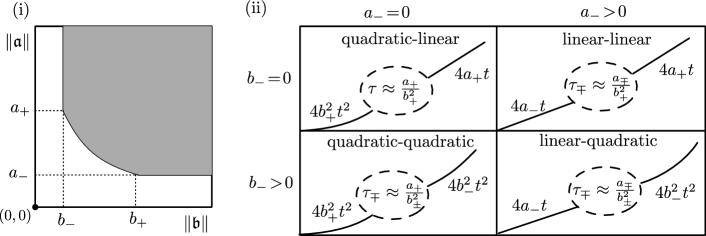
Figure 2: (i) A schematic plot of achievable pairs of operator norms $(\|\mathfrak{a}\,\|\mathfrak{b}\|)$ of operators defined in (4,5). The short-time and asymptotic-time QFI scalings depending on whether the minimal achievable values for $\|\mathfrak{a}\|$ and $\|\mathfrak{b}\|$ are zero or strictly greater then zero—see (ii) part of the figure. The other characteristic points on the plot ${a}_{+}=\min_{h,\|\mathfrak{b}\|={b}_{-}}(\|\mathfrak{a}(h)\|)$, ${b}_{+}=\min_{h,\|\mathfrak{a}\|={a}_{-}}(\|\mathfrak{b}(h)\|)$ represent the minimal values of operator norm of a given operator, assuming the operator norm of the other one is set to its unconstrained minimal value. Given these four numbers, one can write quantitative short-time and asymptotic formulas for the QFI behaviour, as well as assess the relevant time scales when the transition from short-time to asymptotic behaviour takes place (ii).

Furthermore, the formula (2) together with the ‘ab-plot’ allows one to asses the characteristic time-scales when the transition from the short-time to the asymptotic-time scaling regime takes place. It is enough to compare the contributions from the linear and quadratic terms, and find time $\tau$ when they become comparable. In the quadratic-linear case this leads to transition time $\tau\approx\frac{a_{+}}{b_{+}^{2}}$. In three other cases we in fact deal with two time scales, representing the moment when the initial QFI formula ceases to be valid ($\tau_{-}$) and the second time scale when the the QFI approaches the asymptotic behaviour ($\tau_{+}$). These times read $\tau_{\mp}\approx\frac{a_{+}}{b_{\pm}^{2}}$, $\tau_{\mp}\approx\frac{a_{\mp}}{b_{+}^{2}}$ and $\tau_{\mp}\approx\frac{a_{\mp}}{b_{\pm}^{2}}$ for quadratic-quadratic, linear-linear and linear-quadratic models respectively, see Fig. 2(ii).

Algebraic conditions.

While obtaining the exact values of $a_{\pm}$, $b_{\pm}$ requires in general to run an SDP programme, determining whether $a_{-}$, $b_{-}$ are zero or strictly positive may be phrased in terms of simple algebraic conditions on $H$, $\dot{H}$, $\vec{L}$ and $\dot{\vec{L}}$.

Inspecting (4), we see that the condition for the quadratic short-time scaling can be phrased as:

$$a_{-}=0\quad\textrm{iff}\quad\exists_{\mathfrak{h},\vec{h}}\,\dot{\vec{L}}=-i(\mathfrak{h}\vec{L}+\vec{h}\openone).$$ (6)

Looking at (5) it is clear that the condition for linear asymptotic-time scaling amounts to

$$b_{-}=0\quad\textrm{iff}\quad G=\dot{H}-\frac{i}{2}\left(\dot{\vec{L}}^{\dagger}\vec{L}-\vec{L}^{\dagger}\dot{\vec{L}}\right)\in\mathcal{S},$$ (7)

where $\mathcal{S}=\textrm{span}_{\mathbb{C}}\{\openone,L_{k},L_{k}^{\dagger},L_{k}^{\dagger}L_{l}\}$ has been called the Lindblad-span space in [43, 44].

If the parameter is encoded in $H$ only, so $\dot{\vec{L}}=0$, the condition (6) is trivially satisfied and the initial scaling of QFI is always quadratic. The impact of parameter dependence of $L_{k}$ operators on the asymptotic scaling has also been analyzed in [58], but rather than presenting fully general conditions, only some exemplary cases have been discussed.

To investigate the impact of non-zero $\dot{\vec{L}}$ let us discuss first the case when all Lindblad operators’ derivatives are linear combinations of the Lindblad operators themselves. This allows us to write them as:

$$\forall_{i}\dot{L}_{i}\in\textrm{span}_{\mathbb{C}}\{\openone,L_{k}\}\Leftrightarrow\dot{\vec{L}}=\mathfrak{h}_{1}\vec{L}-i\mathfrak{h}_{2}\vec{L}-i\vec{h}\openone,$$ (8)

where $\mathfrak{h}_{1}$ is hermitian matrix, $-i\mathfrak{h}_{2}$ is anti-hermitian matrix, and $-i\vec{h}$ is a complex vector. Thanks to the freedom of redefining $L_{k}$ and $H$, while keeping the quantum master equation unchanged, one can show that there is a representation $H^{\prime}$, $L_{k}^{\prime}$ where the part $-i\mathfrak{h}_{2}$ disappears, while $-i\vec{h}\openone$ part is transferred to the Hamiltonian (see Appendix B):

$$\dot{\vec{L}}^{\prime}=\mathfrak{h}_{1}\vec{L},\quad\dot{H}^{\prime}=\dot{H}-\frac{1}{2}\left[\vec{h}^{\dagger}\vec{L}+\vec{L}^{\dagger}\vec{h}\right].$$ (9)

Hence, only the term $\mathfrak{h}_{1}\vec{L}$ is responsible for the parameter dependence truly connected with the actual dissipative part of the evolution. If this part is non zero, (6) cannot be satisfied. Consequently, we can always interpret the initial quadratic scaling of QFI with a purely Hamiltonian parameter estimation model, while the appearance of linear initial scaling is a clear indication of non-trivial parameter dependence of noise operators $L_{k}$. Moreover, the effective modification of Hamiltonian due to $-i\vec{h}\openone$ term, will not affect the (7) condition as the added term lies in $\mathcal{S}$. Hence, on its own it will never allow for a Heisenberg scaling asymptotic behaviour.

Finally, the interesting case is when at least one of the derivatives $\dot{L}_{i}$ does not live in the span of Lindblad operators $\exists_{i}\dot{L}_{i}\notin\textrm{span}_{\mathbb{C}}\{\openone,L_{k}\}$. Then the second term in (7) provides a nontrivial contribution. In particular, we may even observe asymptotic quadratic QFI scaling, even with no Hamiltonian parameter dependence at all ($\dot{H}=0$) or when the Hamiltonian part on its own would not allow for this–see Examples below.

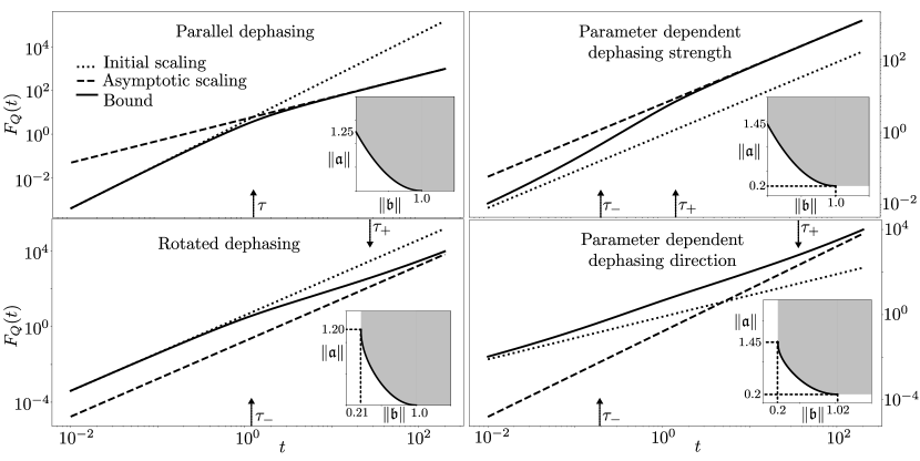
Figure 3: Bound on $F_{Q}(t)$ derived using Eq. (10), as well as initial and asymptotic scalings of $F_{Q}(t)$ as a function of time $t$ in log-log scale for four sensing cases each representing a different initial-asymptotic scaling combination in the same order as depicted in Fig. 2(ii). The insets represent the corresponding ‘ab-plots’ indicating the values of $a_{-}$, $b_{-}$, $a_{+}$, and $b_{+}$. In the the plots, $\tau$, $\tau_{-}$, and $\tau_{+}$ denote the transition times computed according to formulas presented in the schematic Fig. 2(ii). The structure and the numerical parameters for the models are given in Table 1.

Quantitative analysis.

After this qualitative scaling analysis, we now present a recipe to obtain the tightest possible numerical bounds within the framework presented. The method amounts to a discrete time step approximated integration of (2), during which $\|\mathfrak{a}(h)\|$, $\|\mathfrak{b}(h)\|$ are chosen at each step in a way to yield the tightest bound possible. Note that, since we want our bound to be fundamentally valid, we do not assume that control operations can be applied only on time scales longer than the discretization time step $\Delta t$. On the contrary, our bound will be valid for arbitrary fast and arbitrary strong quantum controls, while the choice od the $\Delta t$ will only affect the tightness of the bound—the smaller $\Delta t$ the tighter the bound.

We first note, that RHS of (2) is strictly increasing with time, therefore for any $h$, $F_{Q}(t+\Delta t)-F_{Q}(t)\leq 4(\mathfrak{a}(h)+\mathfrak{b}(h)\sqrt{F_{Q}(t+\Delta t)})\Delta t$. Next, thinking of $F_{Q}(t+\Delta t)$ and $F_{Q}(t)$ as independent variables, we solve the above for $F_{Q}(t+\Delta t)$. Finally, as the obtained inequality is valid for any $h$, we may optimize it over $h$:

$$F_{Q}(t+\Delta t)\leq F_{Q}(t)+4\min_{h}\Big{[}\|\mathfrak{a}(h)\|\Delta t+2\|\mathfrak{b}(h)\|^{2}\Delta t^{2}+\\ \|\mathfrak{b}(h)\|\Delta t\sqrt{F_{Q}(t)+4\|\mathfrak{a}(h)\|\Delta t+4\|\mathfrak{b}(h)\|^{2}\Delta t^{2}}\Big{]}.$$ (10)

Clearly, in the limit $\Delta t\rightarrow 0$ the above formula corresponds to exact integration of $\eqref{QFI-growth}$, but the important point is that for any finite $\Delta t$ it results in a fundamentally valid bound. It is not advisable to optimize $h$ at every step via an SDP. It is much more efficient to first obtain the ‘ab-plot’ or more specifically the curve $a(b)$ connecting $(b_{-},a_{+})$ and $(b_{+},a_{-})$ points, see Fig. 2(i), and then at each step identify the point on the curve $a(b)$ that provides the tightest bound at a given step—this can be done by a simple search through tabularized values of $a(b)$.

Examples.

In Fig. 3 we present numerical results for four models representing all four different ‘scaling cases’, ordered in a way to correspond to classification presented in Fig. 2(ii). The results are presented in log-log scale in order to better reveal the scaling character of the curves. In all the models considered the Hamiltonian is $H(\varphi)=\omega\varphi\sigma_{z}$, and they differ only by the form of the single noise operator $L_{1}(\varphi)$, which is given together with numerical parameters of the models is Table 1. Without loss of generality, we set $\omega=1$ which therefore determines the natural time scale for the problem to be $\omega^{-1}$. We also assume that the parameter to be estimated $\varphi$ is dimensionless, as a result the QFI will also be dimensionless.

model	$L_{1}(\varphi)$	$a_{-}$	$b_{-}$	$a_{+}$	$b_{+}$	$\tau_{-}$	$\tau_{+}$
PD	$\sqrt{\frac{\gamma}{2}}\sigma_{z}$	$\boldsymbol{0}$	$\boldsymbol{0}$	$1.25$	$1$	$1.25$
RD	$\sqrt{\frac{\gamma}{2}}\sigma\!\left(\frac{\pi}{15}\right)$	$\boldsymbol{0}$	$0.21$	$1.20$	$1$	1.20	27.67
PDDS	$\sqrt{\frac{\gamma}{2}}e^{\varphi}\sigma_{z}$	$0.2$	$\boldsymbol{0}$	$1.45$	1	0.2	1.45
PDDD	$\sqrt{\frac{\gamma}{2}}\sigma\!\left(\varphi\right)$	0.2	0.2	1.45	1.02	0.19	36.25

Table 1: The form of the single noise operator $L_{1}$ and the parameters of the models depicted in Fig. 3: PD (parallel dephasing), RD (rotated dephasing), PDDS (parameter dependent dephasing strength), PDDD (parameter dependent dephasing direction), where $\sigma(\theta)=\sigma_{z}\cos\theta+\sigma_{x}\sin\theta$. In all the models $H(\varphi)=\varphi\omega\sigma_{z}$. Numerical values are given for the parameters set to $\omega=1$, $\gamma=0.4$. The sensing is performed around the parameter value $\varphi=0$.

We take the conventional parallel dephasing (PD) model as an example of quadratic-linear case ($a_{-}=0$, $b_{-}=0$). This may be regarded as a generic Hamiltonian parameter estimation case, where noise cannot be removed so that asymptotic Heisenberg scaling is recovered. Consequently, in the plot we note an initial quadratic scaling of $F_{Q}(t)$, which asymptotically goes to linear. Transition time $\tau=\frac{a_{+}}{b_{+}^{2}}=1.25$ is indeed a good indicator of quadratic to linear transition.

For quadratic-quadratic case, we consider a rotated dephasing (RD) model with a parameter independent jump operator $L_{1}=\sqrt{\gamma/2}\sigma\left(\sigma_{z}\cos\frac{\pi}{15}+\sigma_{x}\sin\frac{\pi}{15}\right)$. Here $G=\dot{H}\propto\sigma_{z}\notin\mathcal{S}$ and of course $\dot{L_{1}}=0$. Hence, in this case $a_{-}=0$, but $b_{-}>0$. We have two transition times $\tau_{-}=\frac{a_{+}}{b_{+}^{2}}=1.20$ indicating the transition away from initial quadratic scaling and $\tau_{+}=\frac{a_{+}}{b_{-}^{2}}=27.67$ indicating the transition to asymptotic quadratic scaling.

For the linear-linear case, we consider a the parameter dependent dephasing strength (PDDS) model, where $L_{1}(\varphi)=\sqrt{\gamma/2}e^{\varphi}\sigma_{z}$ depends on $\varphi$. Clearly, condition of Eq. (6) is not satisfied but condition of Eq. (7) is satisfied, meaning $a_{-}>0$, but $b_{-}=0$. Two transition times $\tau_{-}=\frac{a_{-}}{b_{+}^{2}}=0.2$, and $\tau_{+}=\frac{a_{+}}{b_{+}^{2}}=1.45$ faithfully indicates the transition from initial linear scaling to intermediate scaling and then transition to asymptotic linear scaling respectively.

Finally, we consider a parameter dependent dephasing direction (PDDD) model, where $L_{1}(\varphi)=\sqrt{\gamma/2}(\cos{\varphi}\sigma_{z}+\sin{\varphi}\sigma_{x})$. In this model both the conditions of Eq. (6) and Eq. (7) are not satisfied, implying $a_{-}>0$, and $b_{-}>0$ and results in the linear-quadratic scaling case. This model has also been studied in [58] being an example where asymptotic Heisenberg scaling is caused by the parameter dependent jump operator. The two time scales shown in the plot are $\tau_{-}=\frac{a_{-}}{b_{+}^{2}}=0.19$, and $\tau_{+}=\frac{a_{+}}{b_{-}^{2}}=36.25$, which denote the transition from initial linear scaling to intermediate, and ultimately to asymptotic quadratic scaling respectively.

In some situation it is possible to derive an analytical form of the bound obtained via numerical optimization. We provide such an example in Appendix C for the PD case, but stress that in general SDP optimization is necessary to obtain the tightest bound.

Conclusions.

With this paper, we performed comprehensive analysis of general Markovian sensing models and provided simple and efficient tools to assess the potential quantum enhancement for the models on all evolution time-scales. Notice that the framework covers in particular all continuous-measurement paradigms [60, 61] and as such any results obtained in these approaches should obey the bounds derived here. An obvious direction for further research is to study non-Markovian models [62, 63], but this would require going significantly beyond the framework presented here.

Appendix A Semi-definite programme to generate the $(\|\mathfrak{a}\|,\|\mathfrak{b}\|)$-plot

To generate the ‘ab-plot’ plot, first we determine ${a}_{-}=\min_{h}\|\mathfrak{a}(h)\|$ and ${b}_{-}=\min_{h}\|\mathfrak{b}(h)\|$ according to the main text. Next step is to calculate ${b}_{+}=\min_{h,\|\mathfrak{a}\|={a}_{-}}(\|\mathfrak{b}(h)\|)$ and then evaluating $\min_{h}\|\mathfrak{a}\|$, for a given $b\in[b_{-},b_{+}]$. Clearly, given $b=b_{-}$, we get $\min_{h}\|\mathfrak{a}\|=a_{+}$. To be able to do the above calculations, we formulate the following optimization problems,

$${\rm min}_{h}\|\mathfrak{a}\|,\leavevmode\nobreak\ \leavevmode\nobreak\ \text{subject to}\leavevmode\nobreak\ \leavevmode\nobreak\ \|\mathfrak{b}\|\leq b,$$ (11)

$${\rm min}_{h}\|\mathfrak{b}\|,\leavevmode\nobreak\ \leavevmode\nobreak\ \text{subject to}\leavevmode\nobreak\ \leavevmode\nobreak\ \|\mathfrak{a}\|\leq a.$$ (12)

Note that the above minimization problems simply produce $a_{-}$, and $b_{-}$ without any constraints on $\|\mathfrak{b}\|$, and $\|\mathfrak{a}\|$ respectively. We can pose the above optimizations as SDP by constructing the following matrices,

$$A= \begin{pmatrix}a\mathds{1}&{\left(i\dot{\vec{L}}+\mathfrak{h}\vec{L}+\vec{h}\openone\right)}^{\dagger}\\ {\left(i\dot{\vec{L}}+\mathfrak{h}\vec{L}+\vec{h}\openone\right)}&\mathds{1}^{\otimes n}\end{pmatrix},$$ (13)

$$B=\begin{pmatrix}b\mathds{1}&i\mathfrak{b}(h)\\ -i\mathfrak{b}^{\dagger}(h)&b\mathds{1}\end{pmatrix}.$$ (14)

Using the Schur’s complement condition, one can show that, $A\succeq 0\iff a\geq\|\mathfrak{a}\|$, and similarly $B\succeq 0\iff b\geq\|\mathfrak{b}\|$. As a result, just setting the constraint as $A\succeq 0$, and minimizing $a$ is equivalent to minimizing $\|\mathfrak{a}\|$, which gives us $a_{-}$. Similarly, minimizing $b$ with the constraint $B\succeq 0$ is equivalent to minimizing $\|\mathfrak{b}\|$, producing $b_{-}$. Furthermore, minimizing $a$, with two constraints $A\succeq 0$, and $B\succeq 0$, for a given $b$ leads to the solution of the optimization problem defined in Eq. (11). Likewise, minimizing $b$, with the constraints $A\succeq 0$, and $B\succeq 0$ for a given $a$ produces solution of Eq. (12). Clearly, setting $a=a_{-}$, we obtain $b_{+}$. Then we solve Eq. (11), setting $b\in[b_{-},b_{+}]$, and thus producing the ‘ab-plot’.

Appendix B The class of models with effectively only Hamiltonian parameter dependence.

Let us assume that the dynamics of the sensing system is governed by the quantum master equation (1) with Hamilotnian $H$ that has an arbitrary dependence on estimated parameter $\varphi$, and jump operators $\vec{L}$ such that $\dot{\vec{L}}=\mathfrak{h}_{1}\vec{L}-i\mathfrak{h}_{2}\vec{L}-i\vec{h}\openone$. Quantum master equation is invariant under a unitary mixing of jump operators (homogeneous transformation) as well as the inhomogeneous transformation mixing the Hamiltonian with the jump operators [64]:

$$\begin{split}\vec{L}^{\prime}&=u(\varphi)\left[\vec{L}+\vec{v}(\varphi)\openone\right],\\ H^{\prime}&=H+\frac{1}{2i}\left[\vec{v}^{\dagger}(\varphi)\vec{L}-\vec{L}^{\dagger}\vec{v}(\varphi)\right],\end{split}$$ (15)

where $u(\varphi)$ is a $n\times n$ unitary matrix and $\vec{v}(\varphi)\in\mathbb{C}^{n}$. We choose $u(\varphi)=e^{i\mathfrak{h}_{2}\varphi}$ (matrix exponentiation) and $\vec{v}(\varphi)=e^{i\vec{h}\varphi}-\vec{1}$, where we perform element-wise exponentiation and where $\vec{1}$ denotes a vector of length $n$ with all entries equal to $1$. Finally, assuming the derivatives are taken at $\varphi=0$ (this is no loss of generlity as we can always shift the value of parameter in the definition), we get:

$$\dot{\vec{L}}^{\prime}=\mathfrak{h}_{1}\vec{L},\quad\dot{H}^{\prime}=\dot{H}-\frac{1}{2}\left[\vec{h}^{\dagger}\vec{L}+\vec{L}^{\dagger}\vec{h}\right].$$ (16)

As a result, we obtain an equivalent model, where the parameter enters into the Lindblad operator only via hermitian part $\mathfrak{h}_{1}$. If $\mathfrak{h}_{1}=0$, the parameter enters into the Hamiltonian part of the master equation only.

Appendix C Analytical approximately optimal formula for the bounds

In general, we obtain the tightest bound only numerically. Yet, some useful sub-optimal bounds may be easily derived, following the reasoning from [58], adapted to our formalism.

For any $h$ (fixed to be the same during the whole evolution), the inequality:

$$\frac{dF(t)}{dt}\leq 4\|\mathfrak{a}(h)\|+4\|\mathfrak{b}(h)\|\sqrt{F(t)}$$ (17)

may be directly integrated (to a rather complicated form) and further bounded by (Eq. (C17) of [58]):

$$F(t)\leq 4\left(\|\mathfrak{b}(h)\|t+\sqrt{\|\mathfrak{a}(h)\|t}\right)^{2}.$$ (18)

The above bound is valid for any model. In limits $t\to 0$ and $t\to\infty$ it gives respectively $\sim 4\|\mathfrak{a}(h)\|t$ and $\sim 4\|\mathfrak{b}(h)\|^{2}t^{2}$.

For the quadratic-linear case ($a_{-},b_{-}=0$) an analytical bound tighter than above may be derived. Let us name by $h_{a}$, $h_{b}$ a proper $h$ matrices satisfying:

$$\|\mathfrak{a}(h_{b})\|=0,\quad \|\mathfrak{b}(h_{b})\|=b_{+},$$ (19)

$$\|\mathfrak{a}(h_{a})\|=a_{+},\quad \|\mathfrak{b}(h_{a})\|=0.$$ (20)

Then for linear combination $h=\delta h_{a}+(1-\delta)h_{b}$, where $0\leq\delta\leq 1$, we have:

$$\left(i\dot{\vec{L}}+(\delta\mathfrak{h}_{a}+(1-\delta)\mathfrak{h}_{b}\vec{L}+(\delta\vec{h}_{a}+(1-\delta)\vec{h}_{b})\openone\right)=\\ \delta\left(i\dot{\vec{L}}+\mathfrak{h}_{a}\vec{L}+\vec{h}_{a}\openone\right)+\underbrace{(1-\delta)\left(i\dot{\vec{L}}+\mathfrak{h}_{b}\vec{L}+\vec{h}_{b}\openone\right)}_{=0}$$ (21)

so from (4)(5)

$$\|\mathfrak{a}(\delta h_{a}+(1-\delta)h_{b})\|=\quad\delta^{2}\|\mathfrak{a}(h_{a})\| =\quad\delta^{2}a_{+}$$ (22)

$$\|\mathfrak{b}(\delta h_{a}+(1-\delta)h_{b})\|=(1-\delta)\|\mathfrak{b}(h_{b})\| =(1-\delta)b_{+}.$$ (23)

Then (2) takes the form:

$$\frac{dF(t)}{dt}\leq 4\delta^{2}a_{+}+4(1-\delta)b_{+}\sqrt{F(t)}.$$ (24)

RHS may be directly minimized by the choice of $\delta$:

$$\delta=\begin{cases}\frac{b_{+}}{2a_{+}}\sqrt{F(t)}\quad&\textrm{for}\,\frac{2a_{+}}{b_{+}}\leq\sqrt{F(t)},\\ 1\quad&\textrm{for}\,\frac{2a_{+}}{b_{+}}\geq\sqrt{F(t)}.\end{cases}$$ (25)

Then the bound for $F(t)$ may be integrated directly:

$$F(t)\leq\begin{cases}\frac{16a_{+}^{2}}{b_{+}^{2}}(1-2^{-t/t_{c}})^{2}\quad&\textrm{for}\,t\leq t_{c},\\ 4a_{+}(t-t_{c})+4(\frac{a_{+}}{b_{+}})^{2}\quad&\textrm{for}\,t\geq t_{c},\end{cases}$$ (26)

where $t_{c}=\frac{2a_{+}}{b_{+}^{2}}\ln 2$ (for comparison see Eq. (31) of [58], which coincides with our bound after the substituations $a_{+}\leftrightarrow c_{2}$, and $b_{+}\leftrightarrow c_{1}$).

For the PD model considered above, the bound (26) turns out to be as tight as the one obtained by full numerical optimization. This is, however, not the case for all quadratic-linear models, and in principle, for some $t$ the optimal $h(t)$ may be not the one of the form $\delta h_{a}+(1-\delta)h_{b}$.

Similar construction of the bound can be carried out for quadratic-quadratic case leading to the analogous bound as Eq. (37) of [58] with the substitutions $a_{+}\leftrightarrow c_{2}$, $b_{+}\leftrightarrow c_{1}$, and $b_{-}\leftrightarrow c_{0}$. But this bound is not optimal for the RD model in the main text as optimal $h(t)$ is not of the form $\delta h_{a}+(1-\delta)h_{b}$.

Moreover, for linear-linear and linear-quadratic, this method of derivation does not work as there are no counterparts of Eq. (22) and (23) solely in terms of the constants $a_{+}$, $b_{+}$, $a_{-}$, and $b_{-}$. For that we need to use Eq. (10) to obtain the tightest numerical bound, while there is no simple recipe to provide the tightest bound from Eq. (18) in the Ref [58].

References

- Giovannetti et al. [2011] V. Giovannetti, S. Lloyd, and L. Maccone, Nat. Photonics 5, 222 (2011).
- Toth and Apellaniz [2014] G. Toth and I. Apellaniz, J. Phys. A: Math. Theor. 47, 424006 (2014).
- Degen et al. [2017] C. L. Degen, F. Reinhard, and P. Cappellaro, Rev. Mod. Phys. 89, 035002 (2017).
- Braun et al. [2018] D. Braun, G. Adesso, F. Benatti, R. Floreanini, U. Marzolino, M. W. Mitchell, and S. Pirandola, Rev. Mod. Phys. 90, 035006 (2018).
- Pezzè et al. [2018] L. Pezzè, A. Smerzi, M. K. Oberthaler, R. Schmied, and P. Treutlein, Rev. Mod. Phys. 90, 035005 (2018).
- Pirandola et al. [2018] S. Pirandola, B. R. Bardhan, T. Gehring, C. Weedbrook, and S. Lloyd, Nat. Photonics 12, 724 (2018).
- Holevo [2011] A. S. Holevo, Probabilistic and Statistical Aspects of Quantum Theory; 2nd ed., Publications of the Scuola Normale Superiore. Monographs (Springer, 2011).
- Braunstein and Caves [1994] S. L. Braunstein and C. M. Caves, Phys. Rev. Lett. 72, 3439 (1994).
- Chitambar and Gour [2019] E. Chitambar and G. Gour, Rev. Mod. Phys. 91, 025001 (2019).
- Streltsov et al. [2017] A. Streltsov, G. Adesso, and M. B. Plenio, Rev. Mod. Phys. 89, 041003 (2017).
- Horodecki et al. [2009] R. Horodecki, P. Horodecki, M. Horodecki, and K. Horodecki, Rev. Mod. Phys. 81, 865 (2009).
- Schnabel et al. [2010] R. Schnabel, N. Mavalvala, D. E. McClelland, and P. K. Lam, Nature Communications 1, 121 (2010).
- Grote et al. [2013] H. Grote, K. Danzmann, K. L. Dooley, R. Schnabel, J. Slutsky, and H. Vahlbruch, Phys. Rev. Lett. 110, 181101 (2013).
- Tse [2019] M. e. a. Tse, Phys. Rev. Lett. 123, 231107 (2019).
- Sanders and Milburn [1995] B. C. Sanders and G. J. Milburn, Phys. Rev. Lett. 75, 2944 (1995).
- Bollinger et al. [1996] J. J. . Bollinger, W. M. Itano, D. J. Wineland, and D. J. Heinzen, Phys. Rev. A 54, R4649 (1996).
- Huelga et al. [1997] S. F. Huelga, C. Macchiavello, T. Pellizzari, A. K. Ekert, M. B. Plenio, and J. I. Cirac, Phys. Rev. Lett. 79, 3865 (1997).
- Leibfried et al. [2004] D. Leibfried, M. D. Barrett, T. Schaetz, J. Britton, J. Chiaverini, W. M. Itano, J. D. Jost, C. Langer, and D. J. Wineland, Science 304, 1476 (2004).
- Roos et al. [2006] C. F. Roos, M. Chwalla, K. Kim, M. Riebe, and R. Blatt, Nature 443, 316 (2006).
- Jones et al. [2009] J. A. Jones, S. D. Karlen, J. Fitzsimons, A. Ardavan, S. C. Benjamin, G. A. D. Briggs, and J. J. L. Morton, Science 324, 1166 (2009).
- Schmitt et al. [2017] S. Schmitt, T. Gefen, F. M. Stürner, T. Unden, G. Wolff, C. Müller, J. Scheuer, B. Naydenov, M. Markham, S. Pezzagna, J. Meijer, I. Schwarz, M. Plenio, A. Retzker, L. P. McGuinness, and F. Jelezko, Science 356, 832 (2017).
- Hou et al. [2020] Z. Hou, Z. Zhang, G.-Y. Xiang, C.-F. Li, G.-C. Guo, H. Chen, L. Liu, and H. Yuan, Phys. Rev. Lett. 125, 020501 (2020).
- Schmidt et al. [2005] P. O. Schmidt, T. Rosenband, C. Langer, W. M. Itano, J. C. Bergquist, and D. J. Wineland, Science 309, 749 (2005).
- Kruse et al. [2016] I. Kruse, K. Lange, J. Peise, B. Lücke, L. Pezzè, J. Arlt, W. Ertmer, C. Lisdat, L. Santos, A. Smerzi, and C. Klempt, Phys. Rev. Lett. 117, 143004 (2016).
- Hosten et al. [2016] O. Hosten, N. J. Engelsen, R. Krishnakumar, and M. A. Kasevich, Nature 529, 505 (2016).
- Pezzè and Smerzi [2020] L. Pezzè and A. Smerzi, Phys. Rev. Lett. 125, 210503 (2020).
- Kaubruegger et al. [2021] R. Kaubruegger, D. V. Vasilyev, M. Schulte, K. Hammerer, and P. Zoller, Phys. Rev. X 11, 041045 (2021).
- Holland and Burnett [1993] M. J. Holland and K. Burnett, Phys. Rev. Lett. 71, 1355 (1993).
- Lee et al. [2002] H. Lee, P. Kok, and J. P. Dowling, Journal of Modern Optics 49, 2325 (2002).
- Giovannetti et al. [2006] V. Giovannetti, S. Lloyd, and L. Maccone, Phys. Rev. Lett. 96, 010401 (2006).
- Dowling [2008] J. P. Dowling, Contemp Phys 49, 125 (2008).
- Rubin and Kaushik [2007] M. A. Rubin and S. Kaushik, Phys. Rev. A 75, 053805 (2007).
- Shaji and Caves [2007] A. Shaji and C. M. Caves, Phys. Rev. A 76, 032111 (2007).
- Huver et al. [2008] S. D. Huver, C. F. Wildfeuer, and J. P. Dowling, Phys. Rev. A 78, 063828 (2008).
- Olivares and Paris [2007] S. Olivares and M. G. A. Paris, Optics and Spectroscopy 103, 231 (2007).
- Gilbert et al. [2008] G. Gilbert, M. Hamrick, and Y. S. Weinstein, J. Opt. Soc. Am. B 25, 1336 (2008).
- Demkowicz-Dobrzanski et al. [2009] R. Demkowicz-Dobrzanski, U. Dorner, B. J. Smith, J. S. Lundeen, W. Wasilewski, K. Banaszek, and I. A. Walmsley, Phys. Rev. A 80, 013825 (2009).
- Banaszek et al. [2009] K. Banaszek, R. Demkowicz-Dobrzański, and I. A. Walmsley, Nature Photonics 3, 673 (2009).
- Ono and Hofmann [2010] T. Ono and H. F. Hofmann, Phys. Rev. A 81, 033819 (2010).
- Escher et al. [2011] B. M. Escher, R. L. de Matos Filho, and L. Davidovich, Nature Phys. 7, 406 (2011).
- Demkowicz-Dobrzański et al. [2012] R. Demkowicz-Dobrzański, J. Kołodyński, and M. Guţă, Nat. Commun. 3, 1063 (2012).
- Demkowicz-Dobrzański and Maccone [2014] R. Demkowicz-Dobrzański and L. Maccone, Phys. Rev. Lett. 113, 250801 (2014).
- Demkowicz-Dobrzański et al. [2017] R. Demkowicz-Dobrzański, J. Czajkowski, and P. Sekatski, Phys. Rev. X 7, 041009 (2017).
- Zhou et al. [2018] S. Zhou, M. Zhang, J. Preskill, and L. Jiang, Nat. Commun. 9, 78 (2018).
- Zhou and Jiang [2021] S. Zhou and L. Jiang, PRX Quantum 2, 010343 (2021).
- Dür et al. [2014] W. Dür, M. Skotiniotis, F. Fröwis, and B. Kraus, Phys. Rev. Lett. 112, 080801 (2014).
- Kessler et al. [2014] E. M. Kessler, I. Lovchinsky, A. O. Sushkov, and M. D. Lukin, Phys. Rev. Lett. 112, 150802 (2014).
- Arrad et al. [2014] G. Arrad, Y. Vinkler, D. Aharonov, and A. Retzker, Phys. Rev. Lett. 112, 150801 (2014).
- Unden et al. [2016] T. Unden, P. Balasubramanian, D. Louzon, Y. Vinkler, M. B. Plenio, M. Markham, D. Twitchen, A. Stacey, I. Lovchinsky, A. O. Sushkov, M. D. Lukin, A. Retzker, B. Naydenov, L. P. McGuinness, and F. Jelezko, Phys. Rev. Lett. 116, 230502 (2016).
- Sekatski et al. [2017] P. Sekatski, M. Skotiniotis, J. Kołodyński, and W. Dür, Quantum 1, 27 (2017).
- Gorini et al. [1976] V. Gorini, A. Kossakowski, and E. C. G. Sudarshan, Journal of Mathematical Physics 17, 821 (1976).
- Lindblad [1976] G. Lindblad, Communications in Mathematical Physics 48, 119 (1976).
- Helstrom [1976] C. W. Helstrom, Quantum detection and estimation theory (Academic press, 1976).
- Zhang et al. [2022] M. Zhang, H.-M. Yu, H. Yuan, X. Wang, R. Demkowicz-Dobrzański, and J. Liu, Phys. Rev. Res. 4, 043057 (2022).
- Kurdzialek et al. [2024] S. Kurdzialek, P. Dulian, J. Majsak, S. Chakraborty, and R. Demkowicz-Dobrzanski, arXiv e-prints , arXiv:2403.04854 (2024).
- Fujiwara and Imai [2008] A. Fujiwara and H. Imai, J. Phys. A 41, 255304 (2008).
- Pirandola and Lupo [2017] S. Pirandola and C. Lupo, Phys. Rev. Lett. 118, 100502 (2017).
- Wan and Lasenby [2022] K. Wan and R. Lasenby, Phys. Rev. Research 4, 033092 (2022).
- Kurdziałek et al. [2023] S. Kurdziałek, W. Górecki, F. Albarelli, and R. Demkowicz-Dobrzański, Phys. Rev. Lett. 131, 090801 (2023).
- Rossi et al. [2020] M. A. C. Rossi, F. Albarelli, D. Tamascelli, and M. G. Genoni, Phys. Rev. Lett. 125, 200505 (2020).
- Amorós-Binefa and Kołodyński [2021] J. Amorós-Binefa and J. Kołodyński, New Journal of Physics 23, 123030 (2021).
- Chin et al. [2012] A. W. Chin, S. F. Huelga, and M. B. Plenio, Phys. Rev. Lett. 109, 233601 (2012).
- Smirne et al. [2016] A. Smirne, J. Kołodyński, S. F. Huelga, and R. Demkowicz-Dobrzański, Phys. Rev. Lett. 116, 120801 (2016).
- Breuer and Petruccione [2002] H. P. Breuer and F. Petruccione, The Theory of Open Quantum Systems (Oxford University Press, 2002).