Heterogeneous Multi-Agent Reinforcement Learning for Zero-Shot Scalable Collaboration

Abstract

The rise of multi-agent systems, especially the success of multi-agent reinforcement learning (MARL), is reshaping our future across diverse domains like autonomous vehicle networks. However, MARL still faces significant challenges, particularly in achieving zero-shot scalability, which allows trained MARL models to be directly applied to unseen tasks with varying numbers of agents. In addition, real-world multi-agent systems usually contain agents with different functions and strategies, while the existing scalable MARL methods only have limited heterogeneity. To address this, we propose a novel MARL framework named Scalable and Heterogeneous Proximal Policy Optimization (SHPPO), integrating heterogeneity into parameter-shared PPO-based MARL networks. we first leverage a latent network to adaptively learn strategy patterns for each agent. Second, we introduce a heterogeneous layer for decision-making, whose parameters are specifically generated by the learned latent variables. Our approach is scalable as all the parameters are shared except for the heterogeneous layer, and gains both inter-individual and temporal heterogeneity at the same time. We implement our approach based on the state-of-the-art backbone PPO-based algorithm as SHPPO, while our approach is agnostic to the backbone and can be seamlessly plugged into any parameter-shared MARL method. SHPPO exhibits superior performance over the baselines such as MAPPO and HAPPO in classic MARL environments like Starcraft Multi-Agent Challenge (SMAC) and Google Research Football (GRF), showcasing enhanced zero-shot scalability and offering insights into the learned latent representation’s impact on team performance by visualization.

I Introduction

Multi-agent systems are playing more and more important roles in future human society with the development of artificial intelligence [1, 2, 3, 4, 5]. Multi-agent reinforcement learning (MARL) has seen widespread application in cooperative multi-agent tasks across various domains like autonomous vehicle networks [6, 7, 8], guaranteed display ads [9], and video games [10], significantly enhancing collaboration among agents. With the introduction of actor-critic [11] to MARL, recent advances [12, 13] in MARL algorithms exhibit great potential for addressing more complex cooperative tasks in dynamic environments. Despite its successes, traditional MARL methods are confined to specific environments where models are trained. Lack of generalizability poses a significant barrier to real-world deployment.

Specifically, in this paper, we focus on zero-shot scalability and the generalizability of agents’ population sizes. This involves directly applying trained MARL models to other unseen tasks with similar settings but varying numbers of agents without the need for further training, which is necessary in various real-world applications. For instance, traffic flows fluctuate throughout the day, requiring a traffic junction coordination algorithm capable of transferring to scenarios with varying numbers of vehicles.

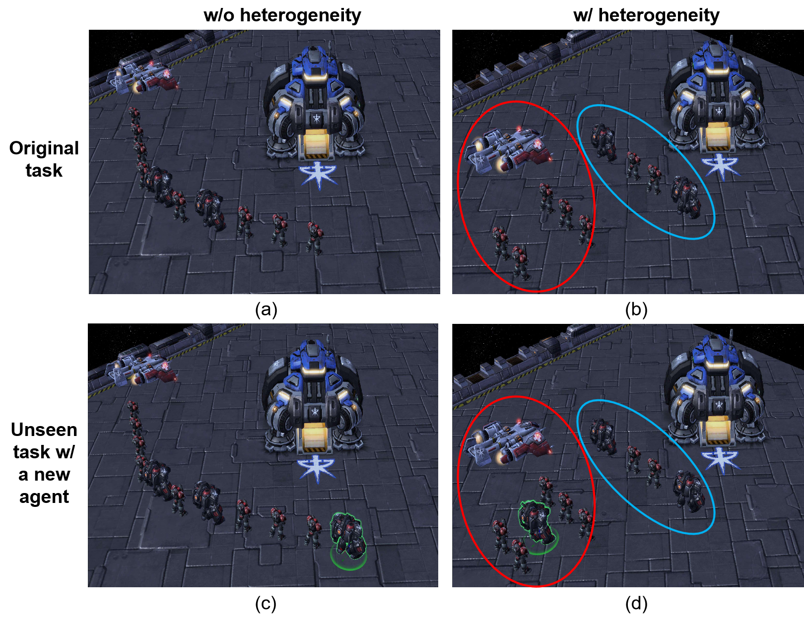
Figure 1: Illustration of scalability and heterogeneity in SMAC. (a) The original task without heterogeneity, where all the agents have the same strategy. (b) The original task with heterogeneity, where the agents form two groups to attract the fire (blue) and attack in the distance (red). (c) The unseen task with a new agent without heterogeneity, where the new agent has the same strategy. (d) The new task with heterogeneity, where the new agent can adaptively choose the strategy.

Moreover, agents within a team may have different strategies or even different functions; thus, learning and transferring heterogeneous roles in a team stands out as an important problem of zero-shot scalable collaboration. First, lack of heterogeneity hinders agents from effectively collaborating with diverse counterparts, constraining team performance. As shown in Fig. 1(a), when heterogeneity is not considered, the agents will have similar strategies and simply form a circle to attack in the game screenshot, while there are different kinds of units with different capacities in the team. But in Fig. 1(b), after the introduction of heterogeneity, some agents may attack in the front to attract the fire (blue circle) while others stay back to be covered. Moreover, in zero-shot scalable tasks, teamwork roles change with team sizes (refer to our experiments in Fig. 8). An adaptive policy is needed to flexibly assign and adjust agents’ heterogeneous roles for better zero-shot scalability. We can implement this policy based on heterogeneous settings (Fig. 1(d)) but may fail without heterogeneity (Fig. 1(c)).

The literature has attempted to address heterogeneity and scalability issues independently. Some works [14, 15] explore giving each agent a distinct model to improve heterogeneity, but they struggle to scale with the number of agents. They suffer from the dimension curse, and there are no training processes for the newly added agents. While other works [16, 17] try to build population-invariant MARL for scalability but ignore the heterogeneity. In addition, parameter sharing is scalable and widely used as network parameters for all agents are shared, bringing benefits of training efficiency and superior performance [18, 19, 20], which, however, also limit the diversity and temporal flexibility of the policies. Motivated by these challenges, we aim to enhance zero-shot scalable collaboration by integrating both inter-individual and temporal heterogeneity.

In this paper, we propose a novel MARL framework called Scalable and Heterogeneous Proximal Policy Optimization (SHPPO) to add a heterogeneous layer to a parameter-shared version of the classic PPO [21] under multi-agent settings (see Fig. 2). We introduce a latent network to adaptively learn low-dimension latent variables to represent the strategy pattern for each agent, according to its observations and trajectories. And then, based on the latent variable, SHPPO generates the parameters of the heterogeneous layer in the actor network. We also introduce a centralized inference net to guide the learning of the latent network to form a symmetrical structure as the actor-critic in PPO (see Fig. 2(b)). Note that our approach can be applied to any parameter-shared MARL backbone, and we take PPO as an example to evaluate the performance in this paper.

In this way, though all the network parameters except for the heterogeneous layers are shared for scalability, the heterogeneous layer for every agent is specifically designed to enhance the diversity of the team. In addition to the inter-individual heterogeneity, the agents are able to update the strategy with the change of observations during the task, so the agents also gain temporal heterogeneity. When transferred to a new scenario with new agents added or removed, the latent variable is accordingly updated with the learned labor division knowledge. Thus the following generation of new heterogeneous layers can transfer the learned strategy patterns while keeping heterogeneity.

By conducting extensive experiments on two classic and complex MARL environments Starcraft Multi-Agent Challenge (SMAC) [22] and Google Research Football (GRF) [23], we demonstrate the superior performance of our method over several baselines such as MAPPO [20] and HAPPO [14]. Thanks to the heterogeneity, our approach shows better zero-shot scalability when directly transferred to scenarios with varied agent populations. Furthermore, we illustrate the learned latent space with the task progress to analyze how heterogeneity improves the team’s performance.

We list the main contributions as follows.

1. New network design: we introduce actor-critic-like latent net and inference net along with corresponding losses to learn latent representations of the agents’ strategy patterns, facilitating the parameter generation of the heterogeneous layer.

2. Novel MARL framework: the proposed approach can add both inter-individual and temporal heterogeneity to any parameter-shared MARL architecture. The flexible and adaptive heterogeneous strategies help the agents scale to unseen scenarios.

3. Superior performance: our method SHPPO outperforms the baselines, such as HAPPO and MAPPO, on the original and zero-shot scalable collaboration tasks of SMAC and GRF.

II Related Works

II-A MARL for Collaboration

Multi-Agent Reinforcement Learning (MARL) has emerged as a powerful paradigm for training groups of AI agents to collaborate and solve complex tasks [6, 7, 8, 9, 10]. QMIX [24] addresses the challenge of credit assignment by computing joint Q-values from individual agents as a value-based method, while MADDPG [12] extends the policy gradient method DDPG [25] to multi-agent settings using centralized critics and decentralized actors. Different from the off-policy MADDPG, MAPPO [20], based on on-policy PPO [21], achieves strong performance in various MARL benchmarks. Despite significant progress, challenges in MARL persist, including generalizability for unseen scenarios, sample efficiency, non-stationarity, and agent communication [26, 27, 28, 29]. In this paper, we mainly focus on zero-shot scalability as one of the generalizability issues.

II-B Scaling MARL

The first step to generalize MARL is to scale the learned MARL models to different population sizes without further training, which is particularly challenging when each agent’s policy is independently modeled [14, 30]. Some works tackle this by designing population-invariant [31], input-length-invariant [32], and permutation-invariant [33] networks. Graph neural networks [34] and transformers [17, 35] are adopted to handle the varying populations. UPDeT [16] further decouples the observation and action space, using an importance weight determined with the aid of the self-attention mechanism. In addition, curriculum learning [31], multi-task transfer learning [36], and parameter sharing [19] are also applied to scale MARL. SePS [18] models all the policies as $K$ parameter-shared networks, and learns a deterministic function to map the agent to one of the policies, which cannot be adaptively updated during the task. In sum, however, these methods all ignore the heterogeneity or limit the heterogeneity to predefined and fixed $K$ policies when scaling MARL, which may lead to ineffective labor division of the agent teams.

II-C Heterogeneous MARL

To implement heterogeneity without separately modeling each agent like HAPPO [14], HetGPPO [37] and CDS [15], existing works have delved into this much to learn the role assignment in MARL [38, 39, 40, 41]. ROMA [42] tailors individual policies based on roles and exclusively depends on the present observation to formulate the role embedding, which may not fully capture intricate agent behaviors. On the other hand, RODE [43] links each role with a specific subset of the complete action space to streamline learning complexity. LDSA [44] introduces heterogeneity from the subtask perspective, but it is hard to determine the total number of subtasks by prior knowledge. Despite these efforts, the existing methods encounter difficulties when scaled to new scenarios with varied population sizes as the number of roles is hard to pre-determine to fit new scenarios, and taking the IDs of agents as inputs to learn the roles makes the integration of a new agent unfeasible. Therefore, achieving a balanced trade-off between scalability and heterogeneity remains an ongoing challenge in MARL.

III Background

III-A DEC-POMDP

We begin by providing an overview of the background related to Markov Decision Processes (MDP) in multi-agent systems. A Markov game [45] is defined by a tuple $<N,S,A,P,r,\gamma>$, where $N=\{1,\ldots,n\}$ represents the set of agents, $S$ denotes the finite state space, $A=\prod_{i=1}^{n}A_{i}$ is the product of finite action spaces for all agents, forming the joint action space. The transition probability function $P:S\times A\times S\rightarrow[0,1]$ and the reward function $r:S\times A\rightarrow\mathbb{R}$ describe the dynamics of the environment, while $\gamma\in[0,1)$ is the discount factor. The agents engage with the environment according to the following protocol: at time step $t\in\mathbb{N}$, the agents find themselves in state $s\in S$; each agent $i$ selects an action $a_{i}\in A_{i}$, drawn from its policy $\pi_{i}(\cdot|s)$; these individual actions collectively form a joint action $\boldsymbol{a}=(a_{1},\ldots,a_{n})\in A$, sampled from the joint policy $\pi(\cdot|s)=\prod_{i=1}^{n}\pi_{i}(\cdot_{i}|s)$; the agents receive a joint reward $r=r(s,\boldsymbol{a})\in\mathbb{R}$ and transition to a new state $s^{\prime}$ with probability $P(s^{\prime}|s,\boldsymbol{a})$. The joint policy $\pi$, transition probability function $P$, and initial state distribution $\rho_{0}$ collectively determine the marginal state distribution at time $t$, denoted by $\rho_{t}^{\pi}$.

In the development of multi-agent reinforcement learning, various paradigms have been introduced to adapt single-agent training methodologies. Initially, the Decentralized Training with Decentralized Execution (DTDE) [46] paradigm is employed, where each agent autonomously makes decisions and learns independently, operating without access to the observations, actions, or policies of other agents. However, this approach encounters the non-stationary problem from the perspective of every single agent when all agents individually update their policies.

To enhance the stability of the learning process, the Centralized Training with Centralized Execution (CTCE) paradigm was introduced [47]. This method conceptualizes the joint policy as a centralized policy and utilizes single-agent methods to learn this aggregated policy. Nonetheless, scalability is hampered by the curse of dimensionality, as the state-action space grows exponentially with the number of agents.

To address this scalability issue, the Centralized Training with Decentralized Execution (CTDE) paradigm [12] combines the advantages of both DTDE and CTCE. CTDE allows agents to utilize additional information during training, yet during execution, each agent acts independently, and decision-making relies solely on its own policy.

When agents are unable to observe the concise state of the environment, commonly referred to as partial observation (PO), a Partially Observable Markov Decision Process (POMDP) extends the MDP model by incorporating observations and their conditional probability of occurrence based on the state of the environment [48, 49]. Within the POMDP and CTDE paradigm, the decentralized partially observable Markov decision processes (DEC-POMDP) [50] have become a widely adopted model in MARL. A DEC-POMDP is defined by $<N,S,A,O,r,P,\gamma>$. $o_{i}=O(s;i)$ represents the local observation for agent $i$ at the global state $s$. Each agent utilizes its policy $\pi_{\theta_{i}}(a_{i}|o_{i})$, parameterized by $\theta_{i}$, to produce an action $a_{i}$ from the local observation $o_{i}$. And agents jointly aim to optimize the discounted accumulated reward $J(\theta)=\mathbb{E}_{\boldsymbol{a},s}[\sum_{t}\gamma^{t}r(s,\boldsymbol{a})]$, where $\boldsymbol{a}$ is the joint action at time step $t$.

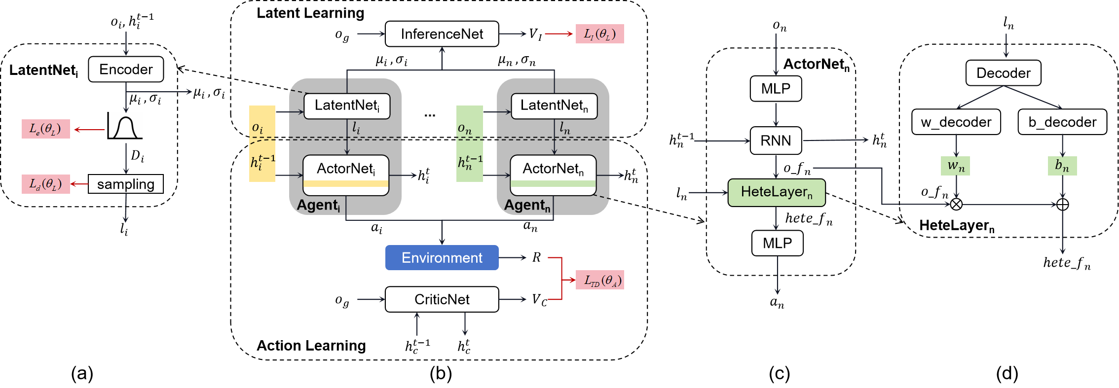
Figure 2: Schematics of our approach SHPPO. (a) Architecture of LatentNet. (b) Framework of SHPPO. (c) Architecture of ActorNet with the heterogeneous layer (HeteLayer). (d) Architecture of HeteLayer. The pink blocks denote the losses. The yellow and green bars denote different HeteLayers.

III-B Policy Gradient (PG)

Policy Gradient (PG) reinforcement learning offers the distinct advantage of explicitly learning a policy network, setting it apart from value-based reinforcement learning methods. PG methods aim to optimize the policy parameter $\theta$ to maximize the objective function $J(\theta)=E_{S}[V_{\pi_{\theta}}(s)]$.

However, choosing an appropriate learning rate in reinforcement learning proves challenging due to the variance of environments and tasks. Suboptimal learning rates may lead to either slow optimization or value collapse, where updated parameters rapidly traverse the current region in policy space.

To address this challenge and ensure stable policy optimization, Trust Region Policy Optimization (TRPO) [51] introduces a constraint on the parameter difference between policy updates. This constraint restricts parameter changes to a small range, preventing value collapse and facilitating monotonic policy learning.

Denote the advantage function as $A(s,\boldsymbol{a})=Q(s,\boldsymbol{a})-R$, with $R=\sum_{t}\gamma^{t}r(s,\boldsymbol{a})$. In the training episode $k$, the parameter update in TRPO follows $\mathop{\theta}_{k+1}={\arg\max}_{\theta}L(\theta_{k},\theta)~{}s.t.\bar{D}_{KL}(\theta||\theta_{k})\leq\delta$, where $L(\theta_{k},\theta)=E[\frac{\pi_{\theta}(a|s)}{\pi_{\theta_{k}}(a|s)}A_{\pi_{\theta_{k}}}(s,a)]$ approximates the original policy gradient objective $J(\theta)$ within the constraint of KL divergence.

Building upon TRPO, Proximal Policy Optimization (PPO) [21] offers a simplified version that maintains the learning step constraint while being more computationally efficient and easier to implement.

In PPO, the objective function is given by:

$$\mathcal{L}(s,a, \theta_{k},\theta)=\mathbb{E}\left[\min\left(\frac{\pi_{\theta}(a|s)}{\pi_{\theta_{k}}(a|s)}A_{\pi_{\theta_{k}}}(s,a),\right.\right.$$ (1)

$$\left.\left.\text{clip}\left(\frac{\pi_{\theta}(a|s)}{\pi_{\theta_{k}}(a|s)},1-\epsilon,1+\epsilon\right)A_{\pi_{\theta_{k}}}(s,a)\right)\right],$$

forcing the ratio $\frac{\pi_{\theta}(a|s)}{\pi_{\theta_{k}}(a|s)}$ to be within the interval $(1-\epsilon,1+\epsilon)$. This ensures that the new parameter $\theta$ remains close to the old parameter $\theta_{k}$.

III-C PG in Multi-agent

Multi-agent PPO (MAPPO) extends PPO to the multi-agent scenario [20], specifically considering DEC-POMDP. MAPPO employs parameter sharing among homogeneous agents, where agents share the same network structure and parameters during both training and testing. MAPPO is a CTDE framework, with each PPO agent maintaining a parameter-shared actor network $\pi_{\theta}$ for policy learning and a critic network $V(s,\phi)$ for value learning, where $\theta$ and $\phi$ are the parameters of the policy and value networks, respectively. The value function requires the global state and is used during training to reduce variance.

MAPPO faces challenges when dealing with heterogeneous agents or tasks and lacks the monotonic improvement guarantee present in trust region learning. To address these limitations, [14] introduced Heterogeneous-Agent TRPO (HATRPO) and Heterogeneous-Agent PPO (HAPPO) algorithms. These algorithms leverage the multi-agent advantage decomposition lemma and a sequential policy update scheme to ensure monotonic improvement. HATRPO/HAPPO extend single-agent TRPO/PPO methods to the context of multi-agent reinforcement learning with heterogeneous agents.

Building on the multi-agent advantage decomposition lemma, HAPPO calculates the actor loss for each agent as follows:

$$\mathcal{L}_{Actor}(\theta)=\mathbb{E}\left[\min\left(\frac{\pi_{\theta^{i_{m}}}^{i_{m}}(a^{i}|s)}{\pi_{\theta_{k}^{i_{m}}}^{i_{m}}(a^{i}|s)}M^{i_{1:m}}(s,\boldsymbol{a}),\right.\right.$$ (2)

$$\left.\left.\text{clip}\left(\frac{\pi_{\theta^{i_{m}}}^{i_{m}}(a^{i}|s)}{\pi_{\theta_{k}^{i_{m}}}^{i_{m}}(a^{i}|s)},1\pm\epsilon\right)M^{i_{1:m}}(s,\boldsymbol{a})\right)\right],$$

where $i_{1:m}$ denotes the permutation of updated $m$ agents, $\theta_{k}^{i_{m}}$ is the network parameter of agent $i_{m}$ in training episode $k$, and $M^{i_{1:m}}(s,\boldsymbol{a})=\prod_{i=1}^{i_{1:m}}\frac{\pi_{\theta^{i}}^{i}(a^{i}|s)}{\pi_{\theta_{k}^{i}}^{i}(a^{i}|s)}(V(s,\phi)-R)$ represents the weighted advantage in HAPPO.

Both MAPPO and HAPPO calculate the critic loss as follows:

$$\mathcal{L}_{Critic}(\phi)=\mathbb{E}\left[(V(s,\phi)-R)^{2}\right].$$ (3)

In our work, we adopt the parameter-shared HAPPO as the baseline and backbone for constructing our approach, SHPPO.

IV Scalable and Heterogeneous
Multi-Agent Reinforcement Learning

Existing heterogeneous MARL methods such as HAPPO model each agent as an independent and different network; it suffers from its inflexibility and huge parameter costs when the scale of the multi-agent system increases. In this section, we propose a novel MARL framework SHPPO and its training method to tackle the trade-off of scalability and heterogeneity.

We try to solve this problem in another direction different from HAPPO: we add adaptive heterogeneity to one single parameter-shared model. Specifically, as in Fig. 2(b), we design the new framework as two parts, latent learning and action learning. First, we implement a latent learning model (LatentNet) to adaptively generate a latent distribution $\mathcal{D}$ for each agent based on its observation and memory (in practice, we take the hidden state of the RNN in the actor network (ActorNet) as the memory). The learned latent distribution represents the strategy pattern of the specific agent, which is further sampled and applied to the computation of the heterogeneous layer parameters for this agent. Except for the heterogeneous layer, the other layers’ parameters in the ActorNet are shared by all the agents. When the number of agents varies, the LatentNet can always generate a unique latent distribution for each agent so that the proposed method can handle the scalability and heterogeneity at the same time. Our approach is agnostic to the implementation of the action learning part, and in practice, we adopt the shared version of HAPPO as the backbone for its monotonic improvement property.

IV-A Scalable Latent Learning

To design a heterogeneous layer for each agent, we first need to represent the agent’s strategy pattern as a low-dimensional latent variable $l$ as shown in Fig. 2(a). Take agent $i$ as an example, we take a 3-layer MLP as the Encoder to convert the observation $o_{i}$ and the memory from the RNN $h^{t-1}_{i}$ at time step $t$ to a latent distribution. Therefore, the Encoder outputs the mean $\boldsymbol{\mu}_{i}$ and the standard deviation $\boldsymbol{\sigma}_{i}$ of the multi-dimensional Gaussian $\boldsymbol{\mathcal{D}}_{i}$. Like humans, the agents’ strategy patterns may not be exactly the same under similar situations, so the Encoder learns a distribution instead of a vector. The final latent variable $l_{i}$ is generated by sampling to keep the randomness as

$$l_{i}\sim\boldsymbol{\mathcal{N}}(\boldsymbol{\mu}_{i},\boldsymbol{\sigma}_{i}).$$ (4)

Inspired by the classic Actor-Critic architecture [11], an inference net (InferenceNet) is introduced as a critic to guide the learning of the LatentNet (see Fig. 2(b)). Though the LatentNet generates the latent variable individually for each agent, the InferenceNet centrally learns an overall value function to evaluate the whole team. Specifically, the InferenceNet takes all the $\boldsymbol{\mu}$ and $\boldsymbol{\sigma}$ as the inputs, together with the joint global observation $o_{g}$, and then computes $V_{I}$ as the evaluation for the LatentNet. The InferenceNet is trained by supervised learning to minimize the difference between $V_{I}$ and the return from the environment $R$. In another way, it judges whether the learned latent distributions are good enough to help with the decision-making based on global observations. Thus, the LatentNet’s goal is to maximize the $V_{I}$.

It is noteworthy that all the agents share the same parameters. Thanks to the CTDE architecture, during the execution and transfer, we only forward the LatentNet and ActorNet, namely, the Agent part in gray color in Fig. 2(b). Though the input dimensions of the InferenceNet and CriticNet vary with the population sizes, this will not influence the transfer to the new scenario to execute. In this way, our method is scalable to fit scenarios with different agent numbers.

IV-B Heterogeneous Layer Design

With the generated latent variable for each agent, we can further design the heterogeneous layer for each agent described in Fig. 2(c, d). The heterogeneous layer is a linear layer in the ActorNet, which also has an MLP and an RNN ahead and an MLP behind. The ActorNet for agent $n$ takes the observation $o_{n}$ and the hidden states of the RNN $h^{t-1}_{n}$ to get the action $a_{n}$. The ActorNet for different agents shares the parameters, except for the heterogeneous layer, whose parameters are generated with each agent’s $l$.

The heterogeneous layer computes $hete\_f_{n}$ as Equation 5.

$$hete\_f_{n}=w_{n}*o\_f_{n}+b_{n}.$$ (5)

Here, the weights $w_{n}$ and the bias $b_{n}$ are unique for different agents, so the decision-making policies are heterogeneous for them. With a decoder implemented as an MLP and two different linear decoders to generate $w_{n}$ and $b_{n}$ based on $l_{n}$, respectively. Namely, the LatentNet learns to represent the strategy patterns, and the heterogeneous layer turns the latent variable into parameters of the ActorNet. Now, the agents can have distinguished styles to take action, though they share most of the parameters. Also, they can change the style adaptively as the task goes on or team size changes. The execution of one time step is shown in Algorithm 1.

Algorithm 1 Execution of one time step $t$.

  Input: observations $\boldsymbol{o}$ and hidden states from the last time step $\boldsymbol{h}^{t-1}$ for all the agents, LatentNet and ActorNet sharing parameters among the agents.

  

  Distributed execution

        Compute latent variable $l_{i}$ by LatentNet with the inputs of $o_{i},h_{i}^{t-1}$ for each agent.

        Compute the parameters $w_{i},b_{i}$ for the HeteLayer in each agent’s ActorNet with the input $l_{i}$.

        Generate the action $a_{i}$ for each agent by ActorNet with $o_{i},h_{i}^{t-1}$ as inputs.

        Store the hidden state $h_{i}^{t}$ for the next step.

  

  Interaction with the environment

        Agents execute the the actions $\boldsymbol{a}$ in the environment together.

        The environment returns the reward $r$ and the flag whether this episode is finished.

IV-C Loss Formulation

A good latent representation should be identifiable, diverse, and helpful for decision-making. Therefore, we design three distinct loss items to guide the learning of the LatentNet.

For the first two demands, we apply unsupervised losses to learn the latent variable. The first item is $\mathcal{L}_{e}$, the mean entropy of the $\boldsymbol{\mathcal{D}}_{i}$, defined as follows:

$$\mathcal{L}_{e}(\theta_{L}) =\frac{1}{n}\sum_{i=1}^{n}\mathcal{H}(\mathcal{D}_{i}(o_{i},h^{t-1}_{i};\theta_{L}))$$

$$=\frac{1}{n}\sum_{i=1}^{n}\mathcal{H}(\mathcal{N}(\boldsymbol{\mu}_{i}(o_{i},h^{t-1}_{i};\theta_{L}),\boldsymbol{\sigma}_{i}(o_{i},h^{t-1}_{i};\theta_{L}))),$$ (6)

where $n$ is the team size, $\mathcal{H}$ is the entropy function of the distribution, $\theta_{L}$ is the parameters of the LatentNet. To minimize the $\mathcal{L}_{e}(\theta_{L})$, the latent distributions tend to be sharper and thus more identifiable.

The second item is the distance among the agents’ latent variables $\mathcal{L}_{d}(\theta_{L})$:

$$\mathcal{L}_{d}(\theta_{L})= \frac{1}{n(n-1)}\sum_{i=1}^{n}\sum_{j\neq i}^{n}Norm(1-$$

$$cos\_sim(l_{i}(o_{i},h^{t-1}_{i};\theta_{L}),l_{j}(o_{j},h^{t-1}_{j};\theta_{L}))),$$ (7)

where $cos\_sim$ is the cosine similarity between two vectors. $Norm$ is the normalization of all the distances to ensure the distance distribution :

$$Norm(x_{i})|_{x_{i}\in\boldsymbol{x}}=\frac{x_{i}-min(\boldsymbol{x})}{max(\boldsymbol{x})-min(\boldsymbol{x})+10^{-12}}.$$ (8)

By maximizing the $\mathcal{L}_{d}(\theta_{L})$, the latent variables will be diverse to encourage the agents to have heterogeneous styles. Note we implement the sampling function as rsample() in Pytorch to get reparameterized samples, so the sampling is differentiable.

The third item is the value $V_{I}$ from the InferenceNet $\mathcal{L}_{v}$:

$$\mathcal{L}_{v}(\theta_{L})= V_{I}(o_{g},\boldsymbol{\mu}(\boldsymbol{o},\boldsymbol{h}^{t-1};\theta_{L}),\boldsymbol{\sigma}(\boldsymbol{o},\boldsymbol{h}^{t-1};\theta_{L})),$$ (9)

where $\boldsymbol{\mu}$ and $\boldsymbol{\sigma}$ are the concatenation of each agent’s $\boldsymbol{\mu}_{i}$ and $\boldsymbol{\sigma}_{i}$. Note that when calculating $\mathcal{L}_{v}(\theta_{L})$ to update the LatentNet, the parameters of the InferenceNet are fixed and will not be updated. To maximize $\mathcal{L}_{v}$, we can expect that the learned latent variables will be improved to help the agents choose a better heterogeneous layer.

Up to this point, we have the overall loss for the LatentNet $\mathcal{L}_{L}(\theta_{L})$ to be minimized as follows,

$$\mathcal{L}_{L}(\theta_{L})=\lambda_{e}\mathcal{L}_{e}(\theta_{L})-\lambda_{d}\mathcal{L}_{d}(\theta_{L})-\lambda_{v}\mathcal{L}_{v}(\theta_{L}),$$ (10)

where $\lambda_{e},\lambda_{d}$, and $\lambda_{v}$ are the weights of the three items of the final loss.

The InferenceNet is learned by an MSE loss between the value $V_{I}$ and environment return $R$:

$$\mathcal{L}_{I}(\theta_{I})= MSE\_Loss[V_{I}(o_{g},\boldsymbol{\mu}(\boldsymbol{o},\boldsymbol{h}^{t-1};\theta_{I}),$$

$$\boldsymbol{\sigma}(\boldsymbol{o},\boldsymbol{h}^{t-1};\theta_{I})),R],$$ (11)

where the MSE loss is calculated as

$$MSE\_Loss[X,Y]=\frac{1}{B}\sum_{k=1}^{B}(x_{k}-y_{k})^{2},$$ (12)

where $B$ is the minibatch size, $x_{k}$ and $y_{k}$ are the samples in the minibatch. The InferenceNet will be able to infer how good the latent distributions are when $\mathcal{L}_{I}$ converges. Then, The value $V_{I}$ will be a good estimation of the return.

Besides, the ActorNet and the CriticNet are updated following the HAPPO loss Equation 2 and Equation 3, including the parameters of the decoder, w_decoder, and b_decoder. The loss of the ActorNet is a Temporal Difference (TD) loss, $\mathcal{L}_{TD}$:

$$\mathcal{L}_{TD}(\theta_{A}) =\mathcal{L}_{Actor}(s,\boldsymbol{a},\theta_{A})$$

$$=\mathcal{L}_{Actor}(V_{C},R,\boldsymbol{a}(\boldsymbol{o},\boldsymbol{h}^{t-1},\boldsymbol{l};\theta_{A})),$$ (13)

note that here $\boldsymbol{l}$ is taken as an input without gradients.

The loss for the critic is $\mathcal{L}_{C}$:

$$\mathcal{L}_{C}(\theta_{C}) =\mathcal{L}_{Critic}(s,\theta_{C})$$

$$=\mathcal{L}_{Critic}(V_{C}(o_{g},h^{t-1}_{c};\theta_{C}),R).$$ (14)

IV-D Overall Training Procedure

In one episode, the first phase is the interaction with the environment to collect data. Every agent gains a latent variable and then decides its action decision at each step (see Algorithm 1). Data such as observations, hidden states, latent variables, actions, and rewards are saved in the buffer. After the agents succeed, fail, or the step limit is reached, the second phase is training (see Algorithm 2). The agents update their ActorNets one by one, following the procedure in HAPPO [14]. Of course, here all the agents share the same ActorNet. Thus, the ActorNet will be updated for $n$ times based on different agents’ observations, actions, and rewards. After that, the CriticNet, the LatentNet, and the InferenceNet update their parameters. Please refer to Appendix  B and C for the detailed network and hyperparameter configurations.

Algorithm 2 Overall Training Procedure.

  Input: batch size $B$, number of agents $n$, number of episodes $K$, max steps per episode $T$.

  Initialize: parameter-shared networks: ActorNet $\{\theta_{A}\}$, CriticNet $\{\theta_{C}\}$, LatentNet $\{\theta_{L}\}$, InferenceNet $\{\theta_{I}\}$, replay buffer $\mathcal{B}$.

  for $k=0:K$ do

        Collect trajectories and latent distributions.

        Push transitions $\{(o^{t}_{i},h^{t-1}_{i},l^{t}_{i},a^{t}_{i},o^{t+1}_{i},r^{t})\},0\leq t\leq T,i=1,...,n$ into $\mathcal{B}$

        Sample a random minibatch of $B$ transitions from $\mathcal{B}$

        Draw a random permutation of agents $i_{1:n}$.

        for agent $i_{m}=i_{1},...,i_{n}$ do

            Update ActorNet as Equation IV-C with $o_{i_{m}},h^{t-1}_{i_{m}},l_{i_{m}}$

        end for

        Update CriticNet as Equation IV-C

        Compute $\mathcal{L}_{e}(\theta_{L}),\mathcal{L}_{d}(\theta_{L})$ by forwarding LatentNet with all the agents’ $\boldsymbol{o}$ and $\boldsymbol{h^{t-1}}$ as Equation IV-C and Equation IV-C.

        Compute $\mathcal{L}_{v}(\theta_{L})$ by InferenceNet as Equation 9.

        Update LatentNet by Equation 10:

            $\mathcal{L}_{L}(\theta_{L})=\lambda_{e}\mathcal{L}_{e}(\theta_{L})-\lambda_{d}\mathcal{L}_{d}(\theta_{L})-\lambda_{v}\mathcal{L}_{v}(\theta_{L})$

        Update InferenceNet by $\mathcal{L}_{I}(\theta_{I})$ as Equation IV-C

  end for

V Experiments

V-A Environments and Metrics

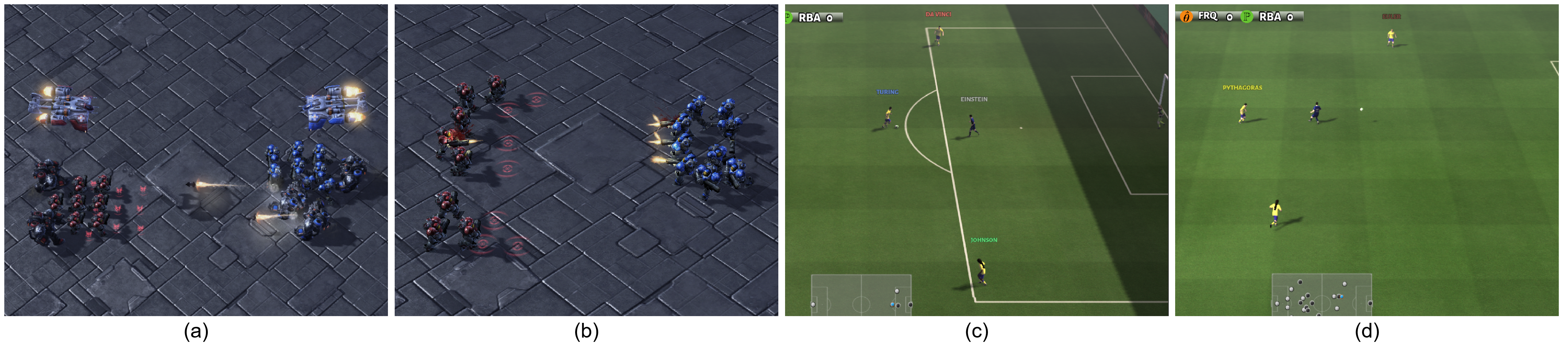
Figure 3: Visualization of the tasks. (a) MMM2 in SMAC. (b) 8m_vs_9m in SMAC. (c) 3_vs_1_with_keeper in GRF. (d) counterattack _easy in GRF.

To demonstrate the effectiveness of our method, especially when scaled to unseen scenarios, we adopt two classic and hard MARL environments - Starcraft Multi-Agent Challenge (SMAC) [22] and Google Research Football (GRF) [23], and further modify them to design scalability tasks.

StarCraft II is a real-time strategy game serving as a classic benchmark in the MARL community. In the Starcraft Multi-Agent Challenge (SMAC) tasks, a team of allied units aims to defeat the adversarial team in various tasks.

Google Research Football (GRF) contains diverse subtasks in a football game. The agents cooperate as part of a football team to score a goal against the opposing team under different scenarios such as counterattack, shooting in the penalty area, etc.

TABLE I: Win/score rate and reward on SMAC and GRF.

Task	Metric	SHPPO		HAPPO		HAPPO (share)*		MAPPO (share)		HATRPO (share)
MMM2	Win rate	71.2$\pm$	6.5	76.3$\pm$	5.1	31.2$\pm$	20.4	62.7$\pm$	10.1	6.8$\pm$	5.9
	Reward	17.5$\pm$	1.3	17.8$\pm$	1.1	14.7$\pm$	3.1	16.9$\pm$	1.5	8.9$\pm$	1.2
8m_vs_9m	Win rate	85.5$\pm$	5.8	81.0$\pm$	10.5	70.5$\pm$	9.3	65.2$\pm$	12.8	78.0$\pm$	8.8
	Reward	18.9$\pm$	0.8	18.3$\pm$	1.2	17.2$\pm$	1.6	17.5$\pm$	1.9	17.5$\pm$	1.5
3_vs_1_with_keeper	Score rate	94.2$\pm$	2.1	90.8$\pm$	2.4	91.3$\pm$	3.7	78.7$\pm$	11.5	41.3$\pm$	20.8
	Reward	19.9$\pm$	0.1	19.6$\pm$	0.2	19.7$\pm$	0.3	17.0$\pm$	1.1	13.3$\pm$	1.3
counterattack_easy	Score rate	91.2$\pm$	3.0	92.0$\pm$	4.1	86.4$\pm$	5.8	81.8$\pm$	7.3	61.4$\pm$	22.5
	Reward	18.9$\pm$	0.2	19.0$\pm$	0.3	18.5$\pm$	0.4	17.3$\pm$	0.5	16.5$\pm$	1.3

• Implemented based on HAPPO but every agent shares the same parameters.

In order to directly zero-shot transfer the learned models to tasks with varied populations, we modify the original environments to fix the number of allies and enemies that one agent can observe. This way, the observations and actions length is the same before and after the transfer. Hence, we can concentrate on transferring strategies without the need to map observations, which is not the primary focus of this paper. For example, in the task MMM2 of SAMC, there are 10 controlled agents and 12 enemies, respectively. In the original tasks of SMAC, the agent can observe all the enemies, resulting in easy and unscalable tasks. We modify the tasks to limit the observation range to the closest 10 enemies and the closest 8 allies so that we can create a series of new tasks with different numbers of agents and enemies to test scalability. While in GRF, there are always 11 players in one team. We change the number of players that the algorithm can control to test scalability but keep the observations as the global observations of all the players in the field. More details of the modified tasks can be found in Appendix Table IV. All the experiments in our paper are conducted on the new scalable tasks.

As for metrics, we adopt training rewards to evaluate the training progress. We also test the performance on the test environments to calculate the win rate for SMAC or score rate for GRF.

We compare the performance of our approach with four other baselines. As SHPPO is built based on parameter-shared HAPPO, we take both HAPPO and HAPPO (share) as baselines. HATRPO [14] is another heterogeneous MARL method, and for a fair comparison, we adopt its parameter-shared version as a baseline. MAPPO [20] is a classic homogeneous MARL method, and in this paper, we also use parameter-shared MAPPO.

V-B Results on SMAC

We first evaluate SHPPO on the original tasks. The first task is a heterogeneous task MMM2, where each side has three kinds of different units - Marine, Marauder, and Medivac (Fig. 3(a)). They have different health points, hit points, and even special skills. Therefore, heterogeneous strategies will improve the team’s performance by maximizing each agent’s advantages. In Fig. 4(a), HAPPO performs best for its great heterogeneous representation ability. However, HAPPO models every agent individually and thus lacks scalability. In contrast, our approach, SHPPO, outperforms all the other parameter-shared baselines without modeling each agent. The training reward and win rate of SHPPO are very close to those of HAPPO, showing that SHPPO has a similar heterogeneous representation ability to HAPPO (See Table I). The performance of the two heterogeneous methods, HAPPO and HATRPO, is the worst when parameters are shared.

We also evaluate on a homogeneous task 8m_vs_9m (Fig. 3(b)), where each side has the same kind of unit - Marine. Though the agents are all the same, they can have different strategies and adaptively alter during the task. As shown in Fig. 4(b) and Table I, SHPPO outperforms all the baselines including HAPPO. The training process of SHPPO also converges faster than other baselines.

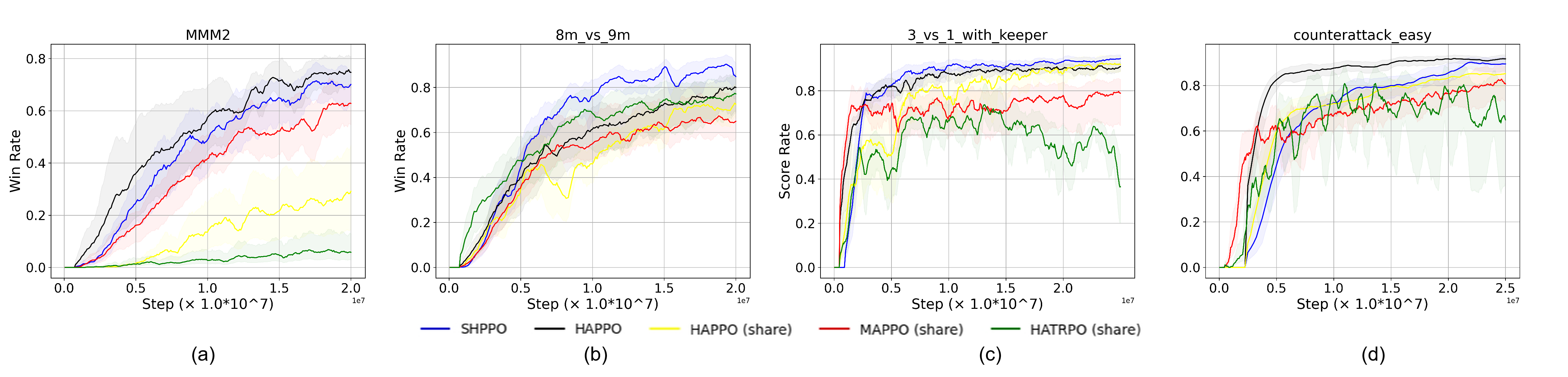
Figure 4: Performance on SMAC and GRF. We plot the win rate on SMAC and the score rate on GRF during training. (a) MMM2 (SMAC). (b) 8m_vs_9m (SMAC). (c) 3_vs_1_with_keeper (GRF). (d) counterattack_easy (GRF). The confidence interval is calculated on 5 seeds.

TABLE II: Scalability test on SMAC.

Task*	SHPPO		HAPPO**		HAPPO (share)		MAPPO (share)		HATRPO (share)
MMM2 (721_831)***	71.2$\pm$	6.5	76.3$\pm$	5.1	31.2$\pm$	20.4	62.7$\pm$	10.1	6.8$\pm$	5.9
722_831	96.3$\pm$	1.5	87.5$\pm$	10.1	95.6$\pm$	2.5	96.1$\pm$	3.8	45.4$\pm$	5.2
821_831	82.5$\pm$	7.5	12.5$\pm$	4.9	70.0$\pm$	19.2	95.1$\pm$	4.5	18.7$\pm$	7.5
731_831	95.6$\pm$	4.5	31.8$\pm$	30.2	96.4$\pm$	3.5	97.5$\pm$	2.5	41.6$\pm$	7.7
711_731	5.6$\pm$	2.5	2.5$\pm$	1.8	0.0$\pm$	0.0	5.1$\pm$	2.5	0.0$\pm$	0.0
711_821	65.8$\pm$	8.2	72.5$\pm$	11.8	35.2$\pm$	17.5	63.5$\pm$	20.1	3.7$\pm$	2.4
621_821	77.5$\pm$	7.8	56.8$\pm$	11.2	25.1$\pm$	12.5	75.2$\pm$	12.5	9.5$\pm$	5.6
621_631	62.5$\pm$	2.5	35.1$\pm$	22.4	26.4$\pm$	14.1	62.5$\pm$	15.9	2.6$\pm$	2.1
8m_vs_9m	85.5$\pm$	5.8	81.0$\pm$	10.5	70.5$\pm$	9.3	65.2$\pm$	12.8	78.0$\pm$	8.8
6m_vs_7m	17.5$\pm$	10.4	2.5$\pm$	1.2	12.7$\pm$	9.8	15.7$\pm$	11.9	12.6$\pm$	8.2
7m_vs_8m	42.5$\pm$	10.7	2.5$\pm$	2.5	40.5$\pm$	10.2	37.1$\pm$	23.5	37.5$\pm$	12.1
10m_vs_11m	70.2$\pm$	20.1	0.0$\pm$	0.0	51.3$\pm$	23.8	42.5$\pm$	18.3	68.1$\pm$	22.5

• The first row is the original task, while the others are unseen tasks with varied numbers of agents, whose results are achieved by zero-shot transfer.

• When transferring HAPPO, We randomly select a model of the same type for the added agent, or removing extra models when there are fewer units in the new task.

• We use the format ABC_DEF to represent the team sizes of both sides. A, B, C are the number of Marines, Marauders, Medivacs of the ally side controlled by our algorithm. D, E, F are the number of Marines, Marauders, Medivacs of the enemy side. The original MMM2 can be represented as 721_831.

V-C Results on GRF

We test the performance on two tasks of GRF. In task 3_vs_1_with_keeper (Fig. 3(c)), our algorithm can control three football players against one adversary player and the keeper. SHPPO is the most effective method among all the methods in Fig. 4(c) and Table I.

In another task counterattack_easy (Fig. 3(d)), four agents need to cooperate together to do a counterattack. They need to pass the ball against one adversary player and the keeper to score. In Fig. 4(d), HAPPO converges fastest and has the best performance. SHPPO reaches a similar performance, though at a slow speed. Still, SHPPO outperforms all the parameter-shared baselines (also see Table I).

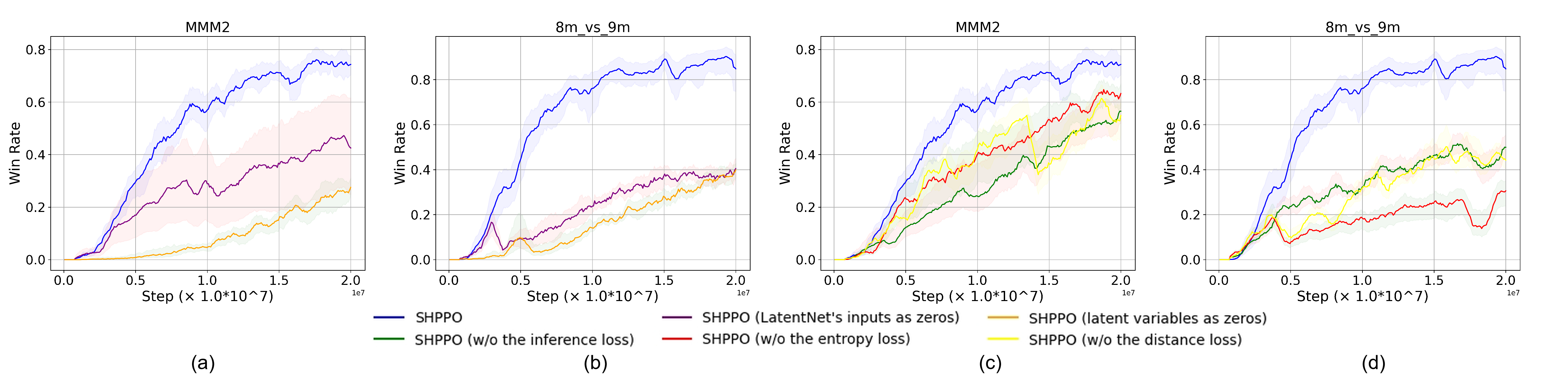
Figure 5: Ablation studies. The experiments are conducted on MMM2 and 8m_vs_9m in SMAC. (a, b) Ablation studies of LatentNet’s inputs. (c, d) Ablation studies of LatentNet’s losses. The confidence interval is calculated on 5 seeds.

TABLE III: Scalability test on GRF.

Task	SHPPO		HAPPO		HAPPO (share)		MAPPO (share)		HATRPO (share)
3_vs_1_with_keeper	94.2$\pm$	2.1	90.8$\pm$	2.4	91.3$\pm$	3.7	78.7$\pm$	11.5	41.3$\pm$	20.8
4_vs_1_with_keeper	90.1$\pm$	9.5	82.3$\pm$	10.7	47.5$\pm$	20.6	61.2$\pm$	15.3	37.8$\pm$	21.5
2_vs_1_with_keeper	92.3$\pm$	7.7	91.0$\pm$	3.5	91.3$\pm$	6.4	63.4$\pm$	22.1	45.2$\pm$	17.3
counterattack_easy* (4_vs_1_counterattack_with_keeper)	91.2$\pm$	3.0	92.0$\pm$	4.1	86.4$\pm$	5.8	81.8$\pm$	7.3	61.4$\pm$	22.5
5_vs_1_counterattack_with_keeper	87.8$\pm$	3.7	89.2$\pm$	4.9	86.5$\pm$	3.4	77.1$\pm$	5.7	68.2$\pm$	12.3
3_vs_1_counterattack_with_keeper	27.4$\pm$	4.1	1.0$\pm$	1.0	24.7$\pm$	5.2	15.1$\pm$	6.5	23.4$\pm$	5.7

• The original task counterattack_keeper can be represented as 4_vs_1_counterattack_with_keeper. The algorithm can control 4 players to counterattack against 1 adversary player and the adversary keeper.

V-D Sacability Test

The proposed method SHPPO not only performs well on the original tasks on SMAC and GRF, but also has extraordinary zero-shot scalability. We construct a series of new tasks with different numbers of agents and enemies to test the scalability.

In the original MMM2 task, the ally team has 7 Marines, 2 Marauders, and 1 Medivac, while the enemy team has 8 Marines, 3 Marauders, and 1 Medivac. This task is labeled as 721_831. To adjust the difficulty of the new task appropriately, we either add one ally unit or remove one ally unit and one enemy unit together. This ensures that the task is neither too difficult nor too easy, avoiding situations where any method would have a win rate of 0% or 100%.

When transferring the learned model from the original task to the unseen tasks, SHPPO does not require additional training. While HAPPO cannot be directly transferred due to each agent having a distinct model, we address this by randomly selecting a model of the same type for the added agent, or removing extra models when there are fewer units in the new task.

From Table II, SHPPO performs the best on most of the unseen zero-shot tasks. Even in cases where SHPPO is not optimal, it still performs comparably to the best. It’s worth noting that although we attempt to transfer HAPPO, it only outperforms SHPPO in one scenario (711_821), despite having a better win rate on the original task.

On another task 8m_vs_9m of SMAC, we also create new tasks with both fewer and more agents, such as 6m_vs_7m and 10m_vs_11m. SHPPO is superior in all the unseen tasks. Surprisingly, HAPPO almost cannot win after the transfer. We suppose that though the agents can have distinct roles in a homogeneous task, their strategies may not be extremely different as they belong to the same unit type. HAPPO possibly overfits every agent’s heterogeneous policy to task 8m_vs_9m, which may not be suitable for the new tasks. Therefore, when we try to transfer HAPPO, the learned strategies do not work on the unseen tasks.

Similarly, we test scalability by removing or adding one agent in the two tasks of GRF. SHPPO maintains the best performance after transfer on the 3_vs_1_with_keeper series. For the counterattack_easy series, despite HAPPO’s best performance on the original task, SHPPO achieves the superior score rate on 3_vs_1_counterattack_with_keeper after the transfer. And when adding a new agent, SHPPO also has comparable performance.

V-E Ablation Studies

We further conduct ablation studies to examine the effects of different parts of latent learning.

In order to test the effectiveness of the latent variables, we first only mask the inputs of the LatentNet with zeros so that the latent variables cannot be adaptively updated according to the new observations. Moreover, in another experiment, we replace all the latent variables with zeros to totally remove the latent learning. In Fig. 5(a, b), when the inputs of LatentNets are zeros, the performance on two tasks of SMAC reduces significantly, especially in task 8m_vs_9m. When the latent variables are set as zeros, it is equal to the removal of the latent learning part, and we can see even worse performance in such a case. Therefore, heterogeneous strategies and flexible adjustment of strategies are important for the agents to cooperate.

Next, we test the effectiveness of the losses of latent learning. We first remove the guidance from the InferenceNet $\mathcal{L}_{v}(\theta_{L})$ while keeping the unsupervised losses $\mathcal{L}_{e}(\theta_{L})$ and $\mathcal{L}_{d}(\theta_{L})$. Results in Fig. 5(c, d) show that without the InferenceNet, there will be a performance decline on both MMM2 and 8m_vs_9m. It suggests that the InferenceNet is able to assess the value of latent variables to help with agents’ decision-making.

Similarly, in Fig. 5(c, d), we then keep $\mathcal{L}_{v}(\theta_{L})$ but remove $\mathcal{L}_{e}(\theta_{L})$ and $\mathcal{L}_{d}(\theta_{L})$, respectively. The two experiments have similar performance reductions on task MMM2. Nevertheless, on the homogeneous task 8m_vs_9m, the experiment without the entropy loss $\mathcal{L}_{e}(\theta_{L})$ has the lowest win rate. We believe this is because, the strategies for a homogeneous task may have some extent of diversity for labor division, but the strategies cannot be too random and different as the agents are of the same unit type. While the entropy loss $\mathcal{L}_{e}(\theta_{L})$ can make sure that the learned latent variables are relatively deterministic and identifiable.

V-F Strategy Analysis

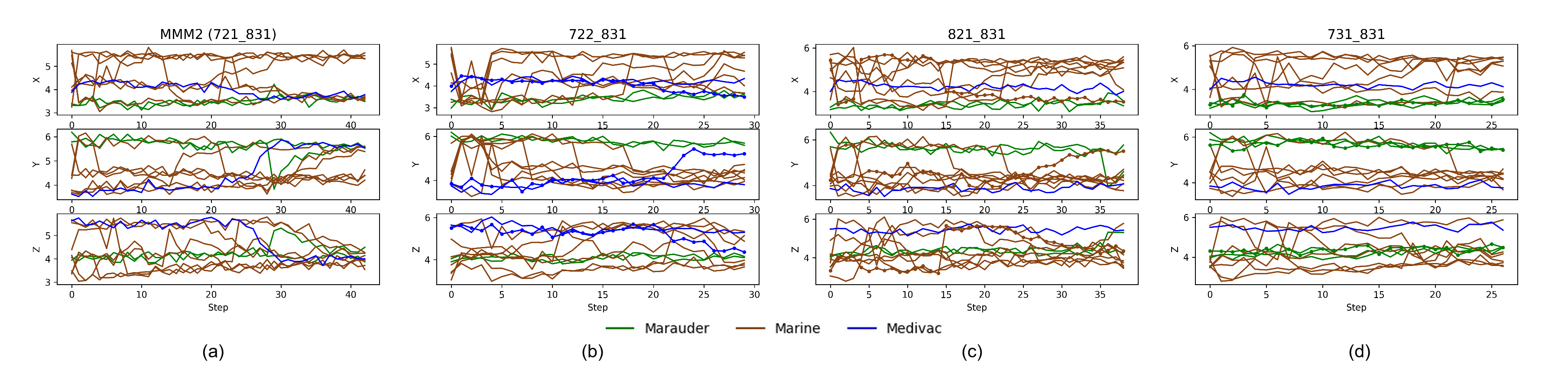
Figure 6: Latent variables in one episode in the original and unseen tasks with different population sizes. The latent variables have three dimensions X, Y, Z and change dynamically with the steps. All the ally agents are illustrated and we use colors to distinguish the unit type. The new agent is marked dots. (a) The original task MMM2. (b) The transferred task 722_831 with a new Medivac. (c) The transferred task 821_831 with a new Marine. (d) The transferred task 731_831 with a new Marauder.

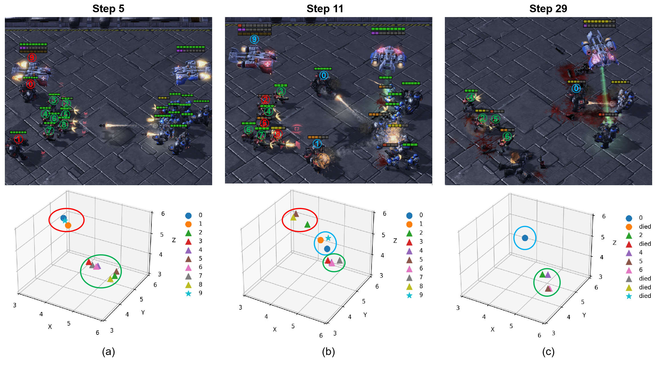
Figure 7: Visualization of MMM2 and latent variables. The agents adaptively adopt different strategies during the task. The latent variables cluster accordingly. Red: stay back to be covered. Green: attack in the distance. Blue: attract the fire by moving to the front.

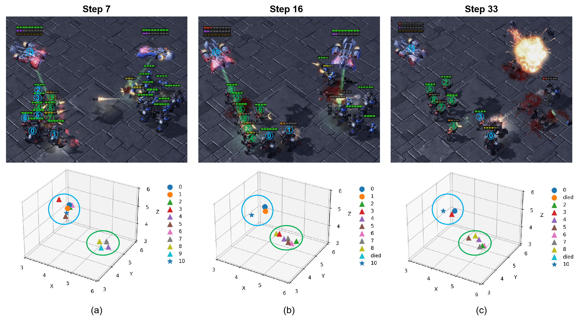
Figure 8: Visualization of the transferred task 821_831 and latent variables. The agents adaptively adjust strategies after being transferred to an unseen task with one added Marine (Number 9). The latent variables cluster accordingly. Green: attack in the distance. Blue: attract the fire by moving to the front.

Finally, we visualize the learned latent variables and the progress of the task to analyze the heterogeneous strategies during the task. Take MMM2 as an example. In Fig. 6, we plot how the latent variables update in one episode. In the original task (Fig. 6(a)), the latent variable patterns vary among different types of units. The two Marauders’ latent variables basically have the same trends, while those of the Marines are much more diverse. Most of the agents do not stick to only one strategy during the task. Instead, they adaptively alter the latent variables to change the strategy. With the learned heterogeneous strategies, we transfer the models to three unseen tasks adding one agent of different types (Fig. 6(b, c, d)). We can see that, generally, the agents’ latent variables still follow similar heterogeneous patterns to those in the original task, with slight differences in strategy updates during the task. Thanks to the shared LatentNet, the newly added agent can initially adopt one of the strategies from units of the same type. However, over time, the new agents may also develop novel strategies to enhance their performance in the new task by temporal heterogeneity (Fig. 6(b) after step 20, Fig. 6(c) after step 15).

We also illustrate the screenshots with the corresponding latent variables before (Fig. 7) and after (Fig. 8) the transfer. In Fig. 7, at the early stage of the task (Step 5), the agents form two groups, the Marines move forward and attack in the front (green circle) to cover the Marauders and the Medivac behind (red circle). At step 11, the two armies encounter and the strategies alter accordingly. The Marauders get close to the enemies to attract the fire while the Medivac keeps curing them (blue circle). Some Marines (Agent 2, 5, and 8) are hurt with low health points, thus they retreat to be covered (red circle), while the other Marines attack the enemies (green circle). In the final stage, some agents are dead and the enemies are almost defeated. The only Marauder keeps attracting the fire in the front. However, the Marines attack the enemies regardless of their health points to achieve final victory.

In Fig. 8, one new Marine is added while the enemies are the same, making the new task easier. Thus, the agents inherit the previous strategies and roles in the team, but further adaptively align them with the easier scenario. At step 7, the added Marine (Agent 9) joins its fellow Marines to attack the enemies (green circle), while other Marines are moving forward to attract and disperse the enemies’ fires, together with the Medivac and Marauders (blue circle). Note that no agents keep staying back to be covered as the red circle in Fig. 7, because they are taking a more aggressive strategy in easier tasks. At step 16, all the Marines stop moving and focus on attacks (green circle). The Marauders go on moving to the front with the support of the Medivac (blue circle). At the final stage (step 33), Marauder 1 dies, and almost at the same time, Marine 3 changes its strategy to replace the dead Marauder, moving to the front (blue circle).

We can see that the latent variables successfully learn the heterogeneous strategy patterns in this task, which are located diversely in the latent space. These latent variables contribute to the adaptive policy updates during the task through the HeteLayer in the ActorNet, so the agents can not only have distinct strategies but also change their strategies as the task progresses and the population size varies.

VI Conclusion

In this paper, we propose a novel MARL framework SHPPO to add both inter-individual and temporal heterogeneity to any parameter-shared actor-critic architecture so that the framework can be scalable for unseen zero-shot new tasks. We introduce latent learning to adaptively update the parameters of the heterogeneous layer and the agents’ strategies. Our approach shows superior performance over baselines, especially for zero-shot scalable collaboration, on several classic MARL tasks. Future work could implement the heterogeneous layer with more complex network designs like transformers, or integrate population-invariant methods to further enhance scalability. One can even take advantage of the emerging large language models (LLMs), converting the latent variables to heterogeneous prompts for LLM agents to gain better scalability.

Appendix A Environment Settings

We modify and keep the number of observations the same in one task series, so that we can focus on the transfer of strategies without mapping the observations. The detailed settings are shown in Table IV.

TABLE IV: Number of observations in the modified tasks for scalability test.

Task	#Obs of allies*	#Obs of enemies
MMM series	9	10
8m_vs_9m series	5	6
3_vs_1_with_keeper series	11	11
counterattack_easy series	11	11

• The number of observations of the ally agents includes the agent itself.

Appendix B Network Settings

We provide the network configurations as follows:

TABLE V: Network configurations for SHPPO.

Module	Implementation
MLP dim	64
Encoder	3-layer MLP
Decoder	3-layer MLP
InferenceNet	3-layer MLP
w_decoder	linear layer
b_decoder	linear layer
HeteLayer	linear layer
ActorNet RNN hidden dim	64
CriticNet RNN hidden dim	64
activation	ReLU
optimizer	Adam
latent variable dim	3

Appendix C Parameter Settings

The hyperparameters used for training of SHPPO is provided in Table VI.

TABLE VI: Hyperparameters settings for SHPPO.

Parameter	Value
mini batch num	1
ActorNet learning rate	0.0005
CriticNet learning rate	0.0005
LatentNet learning rate	0.0005
InferenceNet learning rate	0.005
entropy loss weight $\lambda_{e}$	0.001
distance loss weight $\lambda_{d}$	0.01
inference loss weight $\lambda_{v}$	0.1
discount factor $\gamma$	0.95
evaluate interval	25
evaluate times	40
clip	0.2
GAE lambda	0.95
max steps per episode	160

Appendix D Biography Section

Xudong Guo received the B.Eng. degree in automation from Tsinghua University, Beijing, China, in 2020. He is now pursuing the Ph.D. degree at the Department of Automation, Tsinghua University, Beijing, China. His research interests include multi-agent systems and reinforcement learning.

Daming Shi received the B.S. degree in automatic science from Beihang University, Beijing, China, in 2018 and the Ph.D. degree in automatic science from Tsinghua University, Beijing, China, in 2023. His research interests include reinforcement learning and multi-agent systems in gaming and production.

Junjie Yu received the B.S. degree in automatic science from Beihang University, Beijing, China, in 2023. He is now pursuing the M.S. degree at the Department of Automation, Tsinghua University, Beijing, China. His current research interests include multi-agent systems and reinforcement learning.

Wenhui Fan received the Ph.D. degree in mechanical engineering from Zhejiang University, Hangzhou, China, in 1998. He obtained the postdoctoral certificate from Tsinghua University, Beijing, China, in 2000. He is a vice president of China Simulation Federation. He is currently a professor at Tsinghua University, Beijing, China. His current research interests include multi-agent modeling and simulation, large scale agent modeling and simulation, and multi-agent reinforcement learning.

References

- [1] R. Axelrod and W. D. Hamilton, “The evolution of cooperation,” Science, vol. 211, no. 4489, pp. 1390–1396, 1981.
- [2] V. R. Lesser, “Reflections on the nature of multi-agent coordination and its implications for an agent architecture,” Autonomous agents and multi-agent systems, vol. 1, pp. 89–111, 1998.
- [3] X. Guo, P. Chen, S. Liang, Z. Jiao, L. Li, J. Yan, Y. Huang, Y. Liu, and W. Fan, “Pacar: Covid-19 pandemic control decision making via large-scale agent-based modeling and deep reinforcement learning,” Medical Decision Making, vol. 42, no. 8, pp. 1064–1077, 2022.
- [4] J. S. Park, J. O’Brien, C. J. Cai, M. R. Morris, P. Liang, and M. S. Bernstein, “Generative agents: Interactive simulacra of human behavior,” in Proceedings of the 36th Annual ACM Symposium on User Interface Software and Technology, 2023, pp. 1–22.
- [5] H. Li, Y. Q. Chong, S. Stepputtis, J. Campbell, D. Hughes, M. Lewis, and K. Sycara, “Theory of mind for multi-agent collaboration via large language models,” arXiv preprint arXiv:2310.10701, 2023.
- [6] H. Sha, Y. Mu, Y. Jiang, L. Chen, C. Xu, P. Luo, S. E. Li, M. Tomizuka, W. Zhan, and M. Ding, “LanguageMPC: Large language models as decision makers for autonomous driving,” arXiv preprint arXiv:2310.03026, 2023.
- [7] H. Zhang, S. Feng, C. Liu, Y. Ding, Y. Zhu, Z. Zhou, W. Zhang, Y. Yu, H. Jin, and Z. Li, “CityFlow: A multi-agent reinforcement learning environment for large scale city traffic scenario,” in The World Wide Web Conference. ACM, 2019, pp. 3620–3624.
- [8] J. Wang, T. Shi, Y. Wu, L. Miranda-Moreno, and L. Sun, “Multi-agent graph reinforcement learning for connected automated driving,” in Proceedings of the 37th International Conference on Machine Learning (ICML), 2020, pp. 1–6.
- [9] L. Wang, L. Han, X. Chen, C. Li, J. Huang, W. Zhang, W. Zhang, X. He, and D. Luo, “Hierarchical multiagent reinforcement learning for allocating guaranteed display ads,” IEEE Transactions on Neural Networks and Learning Systems, pp. 1–13, 2021.
- [10] O. Vinyals, I. Babuschkin, W. M. Czarnecki, M. Mathieu, A. Dudzik, J. Chung, D. H. Choi, R. Powell, T. Ewalds, P. Georgiev, J. Oh, D. Horgan, M. Kroiss, I. Danihelka, A. Huang, L. Sifre, T. Cai, J. P. Agapiou, M. Jaderberg, A. S. Vezhnevets, R. Leblond, T. Pohlen, V. Dalibard, D. Budden, Y. Sulsky, J. Molloy, T. L. Paine, C. Gulcehre, Z. Wang, T. Pfaff, Y. Wu, R. Ring, D. Yogatama, D. Wünsch, K. McKinney, O. Smith, T. Schaul, T. Lillicrap, K. Kavukcuoglu, D. Hassabis, C. Apps, and D. Silver, “Grandmaster level in StarCraft II using multi-agent reinforcement learning,” Nature, vol. 575, no. 7782, pp. 350–354, 2019.
- [11] V. Konda and J. Tsitsiklis, “Actor-critic algorithms,” in Advances in Neural Information Processing Systems, vol. 12, 1999.
- [12] R. Lowe, Y. I. Wu, A. Tamar, J. Harb, O. Pieter Abbeel, and I. Mordatch, “Multi-agent actor-critic for mixed cooperative-competitive environments,” Advances in neural information processing systems, vol. 30, 2017.
- [13] S. Iqbal and F. Sha, “Actor-attention-critic for multi-agent reinforcement learning,” in International conference on machine learning. PMLR, 2019, pp. 2961–2970.
- [14] J. G. Kuba, R. Chen, M. Wen, Y. Wen, F. Sun, J. Wang, and Y. Yang, “Trust region policy optimisation in multi-agent reinforcement learning,” arXiv preprint arXiv:2109.11251, 2021.
- [15] C. Li, T. Wang, C. Wu, Q. Zhao, J. Yang, and C. Zhang, “Celebrating diversity in shared multi-agent reinforcement learning,” Advances in Neural Information Processing Systems, vol. 34, pp. 3991–4002, 2021.
- [16] S. Hu, F. Zhu, X. Chang, and X. Liang, “Updet: Universal multi-agent rl via policy decoupling with transformers,” in International Conference on Learning Representations, 2020.
- [17] T. Zhou, F. Zhang, K. Shao, K. Li, W. Huang, J. Luo, W. Wang, Y. Yang, H. Mao, B. Wang et al., “Cooperative multi-agent transfer learning with level-adaptive credit assignment,” arXiv preprint arXiv:2106.00517, 2021.
- [18] F. Christianos, G. Papoudakis, M. A. Rahman, and S. V. Albrecht, “Scaling multi-agent reinforcement learning with selective parameter sharing,” in International Conference on Machine Learning. PMLR, 2021, pp. 1989–1998.
- [19] J. K. Terry, N. Grammel, S. Son, B. Black, and A. Agrawal, “Revisiting parameter sharing in multi-agent deep reinforcement learning,” arXiv preprint arXiv:2005.13625, 2020.
- [20] C. Yu, A. Velu, E. Vinitsky, J. Gao, Y. Wang, A. Bayen, and Y. Wu, “The surprising effectiveness of ppo in cooperative multi-agent games,” Advances in Neural Information Processing Systems, vol. 35, pp. 24 611–24 624, 2022.
- [21] J. Schulman, F. Wolski, P. Dhariwal, A. Radford, and O. Klimov, “Proximal policy optimization algorithms,” arXiv preprint arXiv:1707.06347, 2017.
- [22] M. Samvelyan, T. Rashid, C. Schroeder de Witt, G. Farquhar, N. Nardelli, T. G. Rudner, C.-M. Hung, P. H. Torr, J. Foerster, and S. Whiteson, “The starcraft multi-agent challenge,” in Proceedings of the 18th International Conference on Autonomous Agents and MultiAgent Systems, 2019, pp. 2186–2188.
- [23] K. Kurach, A. Raichuk, P. Stańczyk, M. Zając, O. Bachem, L. Espeholt, C. Riquelme, D. Vincent, M. Michalski, O. Bousquet et al., “Google research football: A novel reinforcement learning environment,” in Proceedings of the AAAI conference on artificial intelligence, vol. 34, no. 04, 2020, pp. 4501–4510.
- [24] T. Rashid, M. Samvelyan, C. S. De Witt, G. Farquhar, J. Foerster, and S. Whiteson, “Monotonic value function factorisation for deep multi-agent reinforcement learning,” The Journal of Machine Learning Research, vol. 21, no. 1, pp. 7234–7284, 2020.
- [25] T. P. Lillicrap, J. J. Hunt, A. Pritzel, N. Heess, T. Erez, Y. Tassa, D. Silver, and D. Wierstra, “Continuous control with deep reinforcement learning,” arXiv preprint arXiv:1509.02971, 2015.
- [26] A. Oroojlooy and D. Hajinezhad, “A review of cooperative multi-agent deep reinforcement learning,” Applied Intelligence, vol. 53, no. 11, pp. 13 677–13 722, 2023.
- [27] Y. Du, J. Z. Leibo, U. Islam, R. Willis, and P. Sunehag, “A review of cooperation in multi-agent learning,” arXiv preprint arXiv:2312.05162, 2023.
- [28] T. T. Nguyen, N. D. Nguyen, and S. Nahavandi, “Deep reinforcement learning for multiagent systems: A review of challenges, solutions, and applications,” IEEE transactions on cybernetics, vol. 50, no. 9, pp. 3826–3839, 2020.
- [29] X. Guo, D. Shi, and W. Fan, “Scalable communication for multi-agent reinforcement learning via transformer-based email mechanism,” in Proceedings of the Thirty-Second International Joint Conference on Artificial Intelligence, IJCAI-23, 2023, pp. 126–134.
- [30] Z. Ding, T. Huang, and Z. Lu, “Learning individually inferred communication for multi-agent cooperation,” Advances in Neural Information Processing Systems, vol. 33, pp. 22 069–22 079, 2020.
- [31] Q. Long, Z. Zhou, A. Gupta, F. Fang, Y. Wu, and X. Wang, “Evolutionary population curriculum for scaling multi-agent reinforcement learning,” arXiv preprint arXiv:2003.10423, 2020.
- [32] W. Wang, T. Yang, Y. Liu, J. Hao, X. Hao, Y. Hu, Y. Chen, C. Fan, and Y. Gao, “From few to more: Large-scale dynamic multiagent curriculum learning,” in Proceedings of the AAAI Conference on Artificial Intelligence, vol. 34, no. 05, 2020, pp. 7293–7300.
- [33] X. Hao, H. Mao, W. Wang, Y. Yang, D. Li, Y. Zheng, Z. Wang, and J. Hao, “Breaking the curse of dimensionality in multiagent state space: A unified agent permutation framework,” arXiv preprint arXiv:2203.05285, 2022.
- [34] A. Agarwal, S. Kumar, and K. Sycara, “Learning transferable cooperative behavior in multi-agent teams,” arXiv preprint arXiv:1906.01202, 2019.
- [35] M. Wen, J. Kuba, R. Lin, W. Zhang, Y. Wen, J. Wang, and Y. Yang, “Multi-agent reinforcement learning is a sequence modeling problem,” Advances in Neural Information Processing Systems, vol. 35, pp. 16 509–16 521, 2022.
- [36] R. Qin, F. Chen, T. Wang, L. Yuan, X. Wu, Z. Zhang, C. Zhang, and Y. Yu, “Multi-agent policy transfer via task relationship modeling,” arXiv preprint arXiv:2203.04482, 2022.
- [37] M. Bettini, A. Shankar, and A. Prorok, “Heterogeneous multi-robot reinforcement learning,” arXiv preprint arXiv:2301.07137, 2023.
- [38] D. Nguyen, P. Nguyen, S. Venkatesh, and T. Tran, “Learning to transfer role assignment across team sizes,” arXiv preprint arXiv:2204.12937, 2022.
- [39] S. Hu, C. Xie, X. Liang, and X. Chang, “Policy diagnosis via measuring role diversity in cooperative multi-agent rl,” in International Conference on Machine Learning. PMLR, 2022, pp. 9041–9071.
- [40] D. Wang, F. Zhong, M. Wen, M. Li, Y. Peng, T. Li, and Y. Yang, “Romat: Role-based multi-agent transformer for generalizable heterogeneous cooperation,” Neural Networks, p. 106129, 2024.
- [41] Z. Hu, Z. Zhang, H. Li, C. Chen, H. Ding, and Z. Wang, “Attention-guided contrastive role representations for multi-agent reinforcement learning,” in The Twelfth International Conference on Learning Representations, 2024.
- [42] T. Wang, H. Dong, V. Lesser, and C. Zhang, “Roma: Multi-agent reinforcement learning with emergent roles,” in International Conference on Machine Learning. PMLR, 2020, pp. 9876–9886.
- [43] T. Wang, T. Gupta, B. Peng, A. Mahajan, S. Whiteson, and C. Zhang, “Rode: learning roles to decompose multi- agent tasks,” in Proceedings of the International Conference on Learning Representations. OpenReview, 2021.
- [44] M. Yang, J. Zhao, X. Hu, W. Zhou, J. Zhu, and H. Li, “Ldsa: Learning dynamic subtask assignment in cooperative multi-agent reinforcement learning,” Advances in Neural Information Processing Systems, vol. 35, pp. 1698–1710, 2022.
- [45] M. L. Littman, “Markov games as a framework for multi-agent reinforcement learning,” in Machine learning proceedings 1994. Elsevier, 1994, pp. 157–163.
- [46] M. Tan, “Multi-agent reinforcement learning: Independent vs. cooperative agents,” in Proceedings of the tenth international conference on machine learning, 1993, pp. 330–337.
- [47] G. Palmer, K. Tuyls, D. Bloembergen, and R. Savani, “Lenient multi-agent deep reinforcement learning,” in Proceedings of the 17th International Conference on Autonomous Agents and MultiAgent Systems, 2018, pp. 443–451.
- [48] L. P. Kaelbling, M. L. Littman, and A. R. Cassandra, “Planning and acting in partially observable stochastic domains,” Artificial intelligence, vol. 101, no. 1-2, pp. 99–134, 1998.
- [49] M. A. Wiering and M. Van Otterlo, “Reinforcement learning,” Adaptation, learning, and optimization, vol. 12, no. 3, p. 729, 2012.
- [50] F. A. Oliehoek, C. Amato et al., A concise introduction to decentralized POMDPs. Springer, 2016, vol. 1.
- [51] J. Schulman, S. Levine, P. Moritz, M. I. Jordan, and P. Abbeel, “Trust region policy optimization,” Computer Science, pp. 1889–1897, 2015.