Dimension-free Relaxation Times of Informed MCMC Samplers on Discrete Spaces

Abstract

Convergence analysis of Markov chain Monte Carlo methods in high-dimensional statistical applications is increasingly recognized. In this paper, we develop general mixing time bounds for Metropolis-Hastings algorithms on discrete spaces by building upon and refining some recent theoretical advancements in Bayesian model selection problems. We establish sufficient conditions for a class of informed Metropolis-Hastings algorithms to attain relaxation times that are independent of the problem dimension. These conditions are grounded in high-dimensional statistical theory and allow for possibly multimodal posterior distributions. We obtain our results through two independent techniques: the multicommodity flow method and single-element drift condition analysis; we find that the latter yields a tighter mixing time bound. Our results and proof techniques are readily applicable to a broad spectrum of statistical problems with discrete parameter spaces.

Keywords: Drift condition; Finite Markov chains; Informed Metropolis-Hastings; Mixing time; Model selection; Multicommodity flow; Random walk Metropolis-Hastings; Restricted spectral gap

1 Introduction

1.1 Convergence of MCMC Algorithms

Approximating probability distributions with unknown normalizing constants is a ubiquitous challenge in data science. In Bayesian statistics, the posterior probability distribution can be obtained through the Bayes rule, but without conjugacy, calculating its normalizing constant is a formidable challenge. In such scenarios, Markov chain Monte Carlo (MCMC) methods are commonly employed to simulate a Markov chain whose stationary distribution coincides with the target distribution. The convergence assessment of MCMC methods usually relies on an empirical diagnosis of Markov chain samples, such as effective sample size (Robert et al., 1999; Gong and Flegal, 2016) and Gelman-Rubin statistic (Gelman and Rubin, 1992), but the results can sometimes be misleading due to the intrinsic difficulty in detecting the non-convergence (Cowles and Carlin, 1996). For this reason, there has been a growing recognition of the importance of taking into account algorithmic convergence when evaluating Bayesian statistical models. A widely used metric for assessing the convergence of MCMC methods is the mixing time, which indicates the number of iterations required for the sampler to get sufficiently close to the target posterior distribution in total variation distance. Most existing studies on the mixing of MCMC algorithms consider Euclidean spaces. In particular, a very rich theory for log-concave target distributions has been developed (Dwivedi et al., 2019; Durmus and Moulines, 2019; Cheng et al., 2018; Dalalyan, 2017; Chewi et al., 2021), providing useful insights into the sampling complexity and guidance on the tuning of algorithm parameters. These results encompass a wide range of statistical models owing to the Bernstein-von Mises theorem (Belloni and Chernozhukov, 2009; Tang and Yang, 2022), which suggests that the posterior distribution becomes approximately normal (and thus log-concave) as the sample size tends to infinity. In contrast, the literature on the complexity of MCMC samplers for discrete statistical models is limited. Further, since every discrete space comes with its own combinatorial structure, researchers often choose to investigate each problem on a case-by-case basis rather than formulating a unified theory for arbitrary discrete spaces. Notable examples include variable selection (Yang et al., 2016), community detection (Zhuo and Gao, 2021), structure learning (Zhou and Chang, 2023), and classification and regression trees (CART) (Kim and Rockova, 2023).

Zhou and Chang (2023) undertook the endeavor to establish a general theoretical framework for studying the complexity of MCMC sampling for high-dimensional statistical models with discrete parameter spaces. They assumed a mild unimodal condition on the posterior distribution, akin to the log-concavity assumption in continuous-space problems, and derived mixing time bounds for random walk Metropolis-Hastings (MH) algorithms that were sharper than existing ones. Here “unimodal” means that other than the global maximizer, every state has a “neighbor” with strictly larger posterior probability, where two states are said to be neighbors if the proposal probability from one to the other is nonzero. Selecting this neighborhood relation often entails a trade-off, and the result of Zhou and Chang (2023) shows that rapid mixing can be achieved if (i) the neighborhood is large enough so that the posterior distribution becomes unimodal, and (ii) the neighborhood is not too large so that the proposal probability of each neighboring state is not exceedingly small. Techniques from high-dimensional statistical theory can be used to establish the unimodality in a way similar to how posterior consistency is proved, but the analysis is often highly complicated and tailored to individual problems. We will not explore these statistical techniques in depth in this paper; instead, our focus will be the mixing time analysis under the unimodal condition or a weaker condition that will be introduced later.

1.2 Main Contributions of This Work

Our first objective is to extend the result of Zhou and Chang (2023) to more sophisticated MH schemes that do not use random walk proposals. We consider the informed MH algorithm proposed in Zanella (2020), which emulates the behavior of gradient-based MCMC samplers on Euclidean spaces (Duane et al., 1987; Roberts and Stramer, 2002; Girolami and Calderhead, 2011) and has gained increasing attention among the MCMC practitioners (Grathwohl et al., 2021; Zhang et al., 2022). The proposal schemes used in the informed algorithms always assess the local posterior landscape surrounding the current state and then tune the proposal probabilities to prevent the sampler from visiting states with low posterior probabilities. However, such informed schemes do not necessarily result in faster mixing, because the acceptance probabilities can be extremely low for proposed states, and it was shown in Zhou et al. (2022) that, for Bayesian variable selection, naive informed MH algorithms can even mix much more slowly than random walk MH algorithms. We will show that this acceptance probability issue can be overcome by generalizing the “thresholding” idea introduced in Zhou et al. (2022). Moreover, if the posterior distribution is unimodal and tails decay sufficiently fast, we prove that there always exists an informed MH scheme whose relaxation time can be bounded by a constant, independent of the problem dimension, which immediately leads to a nearly optimal bound on the mixing time. Our result significantly generalizes the finding of Zhou et al. (2022), which only considered the high-dimensional variable selection problem.

Delving into the more technical aspects, we investigate and compare two different approaches to obtaining sharp mixing time bounds on discrete spaces: the multicommodity flow method (Giné et al., 1996; Sinclair, 1992), and the single-element drift condition (Jerison, 2016). The former bounds the spectral gap of the transition matrix by identifying likely paths connecting any two distinct states. Compared to another path argument, known as “canonical path ensemble” and commonly used in the statistical literature (Yang et al., 2016; Zhuo and Gao, 2021; Kim and Rockova, 2023; Chang et al., 2022), the multicommodity flow method is more flexible and can yield tighter bounds. The drift condition method is based on a coupling argument and stands as the most popular technique for deriving the convergence rates of MCMC algorithms on general state spaces (Rosenthal, 1995; Roy and Hobert, 2007; Fort et al., 2003; Johndrow et al., 2020). A notable difference from the path method is that this approach directly bounds the total variation distance from the stationary distribution without analyzing the spectral gap. The existing literature suggests that both methods have their own unique strengths, and which method yields a better mixing time bound depends on the problem (Jerrum and Sinclair, 1996; Guruswami, 2000; Anil Kumar and Ramesh, 2001). To our knowledge, the two approaches have never been compared for analyzing MCMC algorithms for discrete-space statistical models. Indeed, the only works we are aware of that use drift conditions in these contexts are Zhou et al. (2022) and Kim and Rockova (2023), which considered variable selection and CART, respectively. We will demonstrate how the two methods can be applied under the general framework considered in this paper, and it will be shown that the drift condition approach yields a slightly sharper bound.

As the last major contribution of this work, we further extend our general theory beyond unimodal settings. For multimodal target distributions, while various mixing time bounds have been obtained (Guan and Krone, 2007; Woodard et al., 2009; Zhou and Smith, 2022), it is generally impossible to obtain rapid mixing results where the mixing time grows only polynomially with respect to the problem dimension. This is because the definition of mixing time considers the worst-case scenario regarding the choice of the initial distribution, and the chain can easily get stuck if it is initialized at a local mode. When these local modes (other than the global one) possess only negligible posterior mass and are unlikely to be visited by the sampler given a “warm” initialization, mixing time may provide an overly pessimistic estimate for the convergence rate. One possible remedy was described in the recent work of Atchadé (2021), who proposed to study initial-state-dependent mixing times using restricted spectral gap, a notion that generalizes the spectral gap of a transition matrix, and derived a rapid mixing result for Bayesian variable selection. We extend this technique to our setting and show that it can be integrated with the multicommodity flow method to produce sharp mixing time bounds for both random walk and informed MH schemes.

Setting	Proof techniques	Random walk MH	Informed MH	Require
				warm start
Unimodal	Path method	Thm 1:   $\tau=O\left(M\log\frac{1}{\pi_{\min}}\right)$	Thm 2:   $\tau=O\left(\log\frac{1}{\pi_{\min}}\right)$	No
	Drift condition	Not considered (Remark 6)	Thm 3:   $\tau=O\left(\frac{\log(1/\pi_{\min})}{\log(L/M)}\right)$	No
Beyond	Path method +	Thm 4:   $\tau_{x}=O\left(M\log\frac{1}{\pi(x)}\right)$	Thm 5:   $\tau_{x}=O\left(\log\frac{1}{\pi(x)}\right)$	Yes
unimodal	restricted spectral gap

Table 1: Mixing time bounds obtained in this paper. Here, $\pi$ is the target posterior distribution, $\pi_{\min}=\min_{x}\pi(x)$, $M$ is the maximum neighborhood size, and $L$ is a parameter of the informed proposal scheme. Mixing times $\tau$ and $\tau_{x}$ are defined in (10) and (9) respectively, where $\epsilon$ is treated as fixed. See theorem statements for the required assumptions.

1.3 Organization of the Paper

In Section 2, we review some recent results about the Bayesian variable selection problem, which will be used as an illustrative example throughout this paper; this section can be skipped for knowledgeable readers. Section 3 presents the setup for our theoretical analysis and reviews the mixing time bounds for random walk MH algorithms. In Section 4, we consider unimodal target distributions and prove mixing time bounds for informed MH algorithms via both the path method and drift condition analysis. Section 5 generalizes our results to a potentially multimodal setting. Simulation studies are conducted in Section 6, and Section 7 concludes the paper with some further discussion. A summary of the mixing time bounds obtained in this work is presented in Table 1.

Most technical details are deferred to the appendix. In Appendix A, we review the path method used in Zhou and Chang (2023) for bounding the spectral gaps of MH algorithms. In Appendix B, we review the result about restricted spectral gaps obtained in Atchadé (2021) and develop the multicommodity flow method for bounding restricted spectral gaps. Appendix C gives a brief review of the single-element drift condition of Jerison (2016). Proofs for all results presented in the main text are given in Appendix D.

2 Working Example: Variable Selection

We review in this section some recent advancements in understanding the complexity of MCMC sampling for high-dimensional spike-and-slab variable selection, one of the most representative examples for discrete-space models in Bayesian statistics (Tadesse and Vannucci, 2021).

2.1 Target Posterior Distribution

We consider the standard linear regression model where a design matrix $\bm{X}\in\mathbb{R}^{n\times p}$ and a response vector $\bm{y}\in\mathbb{R}^{n}$ are assumed to satisfy

$$\bm{y}=\bm{X}\bm{\beta}^{*}+\bm{z},\quad\bm{z}\sim\mathrm{MVN}(0,\sigma^{2}\bm{I}_{n}),$$ (1)

where $\bm{\beta}^{*}\in\mathbb{R}^{p}$ is the unknown vector of regression coefficients and $\mathrm{MVN}$ denotes the multivariate normal distribution. Introduce the indicator vector $\delta=(\delta_{1},\dots,\delta_{p})\in\{0,1\}^{p}$ such that $\delta_{j}=1$ indicates that the $j$-th variable has a non-zero effect on the response. Variable selection is the task of identifying the true value of $\delta$, that is, finding the subset of variables with nonzero regression coefficients. Given $\delta$, we can write $\bm{y}=\bm{X}_{\delta}\bm{\beta}_{\delta}+\bm{z}$ with $\bm{z}\sim\mathrm{MVN}(0,\sigma^{2}\bm{I}_{n})$, where $\bm{X}_{\delta}$ and $\bm{\beta}_{\delta}$, respectively, denote the submatrix and subvector corresponding to those variables selected in $\delta$. We will also call $\delta\in\mathcal{V}$ a model, and $\delta=(0,0,\dots,0)$ will be referred to as the empty model. Consider the following two choices for the space of allowed models:

$$\mathcal{V}=\{0,1\}^{p},\text{ or }\mathcal{V}_{s}=\{\delta\in\mathcal{V}\colon||\delta||_{1}\leq s\},$$ (2)

where $||\cdot||_{1}$ denotes the $L^{1}$-norm and $s$ is a positive integer. The set $\mathcal{V}$ is the unrestricted space, while $\mathcal{V}_{s}$ represents a restricted space with some sparsity constraint. Let $|\cdot|$ denote the cardinality of a set. It is typically assumed in the high-dimensional literature that the sparsity parameter $s$ increases to infinity with $p$, in which case both $|\mathcal{V}|=2^{p}$ and $|\mathcal{V}_{s}|=O(p^{s})$ grow super-polynomially with $p$.

Spike-and-slab variable selection is a Bayesian procedure for constructing a posterior distribution over $\mathcal{V}$ or $\mathcal{V}_{s}$, which we denote by $\pi(\delta)$. In Section 6.1, we recall one standard approach to specifying the prior distribution for $(\delta,\bm{\beta},\sigma^{2})$, which leads to the following closed-form expression for $\pi$ up to a normalizing constant.

$$\quad\pi(\delta)\propto\frac{1}{p^{\kappa||\delta||_{1}}}\cdot\frac{(1+g)^{-(||\delta||_{1}/2)}}{\left(1+g\left(1-\mathsf{r}^{2}(\delta)\right)\right)^{n/2}}.$$ (3)

In (3), $\kappa,g$ are prior hyperparameters and $\mathsf{r}^{2}(\delta)=\bm{y}^{\top}(\bm{X}_{\delta}(\bm{X}_{\delta}^{\top}\bm{X}_{\delta})^{-1}\bm{X}_{\delta}^{\top})\bm{y}/(\bm{y}^{\top}\bm{y})$ is the coefficient of determination. Exact calculation of the normalizing constant is usually impossible, because it would require a summation over the entire parameter space, which involves super-polynomially many evaluations of $\pi$.

2.2 MH Algorithms for Variable Selection

To find posterior probabilities of models of interest or evaluate integrals with respect to $\pi$, the most commonly used method is to use an MH algorithm to generate samples from $\pi$. The transition probability from $\delta$ to $\delta^{\prime}$ in an MH scheme can be expressed by

$$\mathsf{P}(\delta,\delta^{\prime})=\mathsf{K}(\delta,\delta^{\prime})\mathsf{A}(\delta,\delta^{\prime}),$$

where $\mathsf{K}(\delta,\delta^{\prime})$ is the probability of proposing to move from $\delta$ to $\delta^{\prime}$, and the associated acceptance probability $\mathsf{A}(\delta,\delta^{\prime})$ is given by

$$\mathsf{A}(\delta,\delta^{\prime})=\min\left\{1,\frac{\pi(\delta^{\prime})\mathsf{K}(\delta^{\prime},\delta)}{\pi(\delta)\mathsf{K}(\delta,\delta^{\prime})}\right\},$$ (4)

ensuring that $\pi$ is the stationary distribution of $\mathsf{P}$.

The efficiency of the MH algorithm depends on the choice of $\mathsf{K}$, and there are many strategies for selecting the proposal neighborhood and assigning the proposal probabilities. Recall that neighborhood refers to the support of the distribution $\mathsf{K}(\delta,\cdot)$ for each $\delta$, which we denote by $\mathcal{N}(\delta)$. Let us begin by considering random walk proposals such that $\mathsf{K}(\delta,\cdot)$ is simply the uniform distribution on $\mathcal{N}(\delta)$. To illustrate the importance of selecting a proper proposal neighborhood, we first present two naive choices that are bound to result in slow convergence.

Example 1.

Let the state space be $\mathcal{V}$ and the proposal $\mathsf{K}(\delta,\cdot)$ be a uniform distribution on $\mathcal{N}(\delta)=\mathcal{V}$ for each $\delta$. In this case, we get an independent MH algorithm, which is clearly ergodic but usually mixes very slowly. For example, suppose the true model is $\delta^{*}=(1,0,0,\dots,0)$ and the data is extremely informative. Even if the chain is initialized at the empty model, it takes on average $2^{p}$ iterations to propose moving to $\delta^{*}$.

Example 2.

Let $T\colon\mathcal{V}\rightarrow\{0,1,\dots,2^{p}-1\}$ be a one-to-one mapping defined by $T(\delta)=\sum_{j=1}^{p}\delta_{j}2^{j-1}$. Define $\mathcal{N}(\delta)=T^{-1}(\{T(\delta)+1,T(\delta)-1\})$. In words, we number all elements of $\mathcal{V}$ from $0$ to $2^{p}-1$, and the proposal is a simple random walk on $\{0,1,\dots,2^{p}-1\}$. The resulting MH algorithm is also ergodic, but again the mixing is slow, since it requires at least $2^{p}-1$ steps to move from the empty model to the full model $(1,1,\dots,1)$.

The neighborhood size is exponential in $p$ in Example 1 and is a fixed constant in Example 2. Both are undesirable, and it is better to use a neighborhood with size polynomial in $p$. The following choice is common in practice:

$$\mathcal{N}_{1}(\delta)=\{\delta^{\prime}\in\mathcal{V}\colon||\delta-\delta^{\prime}||_{1}=1,\text{ and }\delta\neq\delta^{\prime}\}.$$ (5)

The set $\mathcal{N}_{1}(\delta)$ contains all the models that can be obtained from $\delta$ by either adding or removing a variable. When the design matrix $\bm{X}$ contains highly correlated variables, it is generally considered that $\mathcal{N}_{1}$ is too small and introducing “swap” moves is beneficial, which means to remove one variable and add another one at the same time. The resulting random walk MH algorithm is often known as the add-delete-swap sampler; denote its neighborhood by $\mathcal{N}_{\rm{ads}}$, which is defined by

$$\mathcal{N}_{\rm{ads}}(\delta)=\mathcal{N}_{1}(\delta)\cup\mathcal{N}_{\mathrm{swap}}(\delta),\quad\mathcal{N}_{\mathrm{swap}}(\delta)=\left\{\delta^{\prime}\in\mathcal{V}\colon||\delta^{\prime}-\delta||_{1}=2,||\delta^{\prime}||_{1}=||\delta||_{1}\right\}.$$ (6)

We will treat $\mathcal{N}_{\rm{ads}}$ and $\mathcal{N}_{1}$ as neighborhood relations defined on $\mathcal{V}$. When implementing the add-delete-swap sampler on the restricted space $\mathcal{V}_{s}$, one can still propose $\delta^{\prime}$ from $\mathcal{N}_{\rm{ads}}(\delta)$ and simply reject the proposal if $\delta^{\prime}\notin\mathcal{V}_{s}$. Note that $|\mathcal{N}_{\rm{ads}}(\delta)\cap\mathcal{V}_{s}|=O(ps)$.

We end this subsection with two comments. First, a popular alternative to MH algorithms is Gibbs sampling. Consider a random-scan Gibbs sampler that randomly picks $j\in\{1,2,\dots,p\}$ and updates $\delta_{j}$ from its conditional posterior distribution given the other coordinates. It is not difficult to see that this updating is equivalent to randomly proposing $\delta^{\prime}\in\mathcal{N}_{1}(\delta)$ and accepting $\delta^{\prime}$ with probability $\pi(\delta^{\prime})/(\pi(\delta)+\pi(\delta^{\prime}))$. By Peskun’s ordering (Mira, 2001), this Gibbs sampler is less efficient than the random walk MH algorithm with proposal neighborhood $\mathcal{N}_{1}$ (George and McCulloch, 1997).

Second, for simplicity, we assume in this work that $\mathsf{K}(\delta,\cdot)$ is a uniform distribution on $\mathcal{N}(\delta)$ for random walk proposals. But in practice, these proposals can be implemented in a more complicated, non-uniform fashion. For example, one can first choose randomly whether to add or remove a variable, and then given the type of move, a proposal of that type is generated with uniform probability. This distinction has minimal impact on all theoretical results we will develop.

2.3 Rapid Mixing of a Random Walk MH Algorithm

The seminal work of Yang et al. (2016) considered a high-dimensional setting with $n,p,s\rightarrow\infty$ and $s\log p=o(n)$, and they proved that, under some mild assumptions, the mixing time of the add-delete-swap sampler on the restricted space $\mathcal{V}_{s}$ has order $O(pns^{2}\log p)$, polynomial in $(n,p,s)$; in other words, the sampler is rapidly mixing. To provide intuition about this result and proof techniques, which will be crucial to the understanding of the theory developed in this work, we construct a detailed illustrative example.

Example 3.

Let $p=3$ and $\bm{X}$ be such that $||\bm{X}_{j}||_{2}^{2}=n$ for $j=1,2,3$, $\bm{X}_{1}^{T}\bm{X}_{2}=-0.8n$, $\bm{X}_{2}^{T}\bm{X}_{3}=-0.6n$ and $\bm{X}_{1}^{T}\bm{X}_{3}=0.9n$; the three explanatory variables are highly correlated. Let $\bm{y}$ be generated by

$$\bm{y}=1.25\bm{X}_{1}+\bm{X}_{2}+\bm{z},$$

where $\bm{z}$ is orthogonal to each explanatory variable, i.e., $\bm{X}_{j}^{\top}\bm{z}=0$ for each $j$, and $||\bm{z}||_{2}^{2}=n$. We calculate the un-normalized posterior probabilities by (3) for all models with $n=1,000$, $g=p^{3}=27$ and $\kappa=1$; the values are given in Table 2.

$\delta$	$1-\mathsf{r}^{2}(\delta)$	$C+\log\pi(\delta)$	Local mode	Local mode	Local mode
			w.r.t. $(\mathcal{V},\mathcal{N}_{1})$	w.r.t. $(\mathcal{V}_{2},\mathcal{N}_{1})$	w.r.t. $(\mathcal{V}_{2},\mathcal{N}_{\mathrm{ads}})$
$(0,0,0)$	1	0	No	No	No
$(1,0,0)$	0.8704	63.98	No	No	No
$(0,1,0)$	1	-2.76	No	No	No
$(0,0,1)$	0.8236	90.46	No	No	No
$(1,1,0)$	0.64	207.70	Global mode	Global mode	Global mode
$(1,0,1)$	0.8219	88.69	No	No	No
$(0,1,1)$	0.7243	148.95	No	Yes	No
$(1,1,1)$	0.64	204.90	No	–	–

Table 2: Log-posterior probabilities of all possible models in Example 3 with $n=1,000$, $g=p^{3}=27$ and $\kappa=1$. For the third column, we set the constant $C=-\log\pi((0,0,0))$. For each $\delta$, we indicate if it is a local mode with respect to the given search space and neighborhood relation.

The true model, $\delta^{*}=(1,1,0)$, is the global mode of $\pi$, which is expected since $p$ is small but $n$ is large. Further, we indicate in Table 2 if each model is a local mode with respect to the given search space and neighborhood relation. For example, we say $\delta\in\mathcal{V}_{2}$ is a local mode with respect to $(\mathcal{V}_{2},\mathcal{N}_{\rm{ads}})$ if $\pi(\delta)>\pi(\delta^{\prime})$ for every $\delta^{\prime}\in\mathcal{V}_{2}\cap\mathcal{N}_{\rm{ads}}(\delta)$. When there is only one local mode (which must be $\delta^{*}$ in this example), we say $\pi$ is unimodal. Table 2 shows that $\pi$ is unimodal with respect to $(\mathcal{V}_{2},\mathcal{N}_{\mathrm{ads}})$, but it is multimodal with respect to $(\mathcal{V}_{2},\mathcal{N}_{1})$ and the other local mode is $(0,1,1)$. A graphical illustration is given in Figure 1. Another interesting observation is that $\pi(\delta)$ does not necessarily increase as $\delta$ gets closer to $\delta^{*}$. We have $\pi((0,0,1))>\pi((0,0,0))>\pi((0,1,0))$, while the $L^{1}$ distance from each of the three models to $\delta^{*}$ is strictly decreasing. This happens due to the correlation structure among the three variables, and in high-dimensional settings, such collinearity is very likely to occur between some variables. We will frequently revisit this example in later discussions.

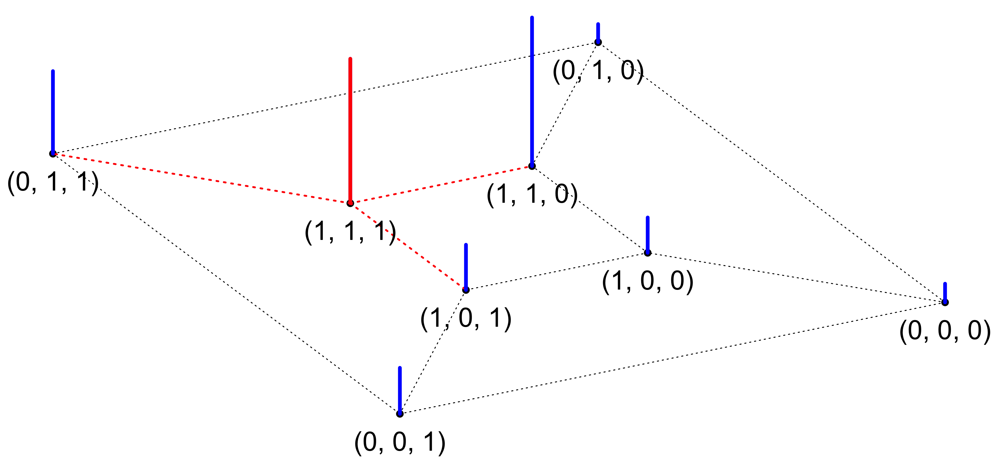
Figure 1: Visualization of $\pi$ on $(\mathcal{V},\mathcal{N}_{1})$ in Example 3. For every $\delta\in\mathcal{V}$, the neighboring states $\delta^{\prime}\in\mathcal{N}_{1}(\delta)$ are connected by dotted lines. The height of each bar is equal to $\sqrt[100]{\pi(\delta)}$. The red bar and dotted lines are removed if the underlying space is $(\mathcal{V}_{2},\mathcal{N}_{1})$.

In Example 3, $\pi$ is unimodal with respect to $(\mathcal{V}_{2},\mathcal{N}_{\mathrm{ads}})$. An important intermediate result of Yang et al. (2016) was that, with high probability, such a unimodality property still holds in the high-dimensional regime they considered, and the global mode coincides with the true model $\delta^{*}$. This implies that the add-delete-swap sampler is unlikely to get stuck at any $\delta\neq\delta^{*}$, since there always exists some neighboring state $\delta^{\prime}$ such that $\mathsf{A}(\delta,\delta^{\prime})=1$ and thus $\mathsf{P}(\delta,\delta^{\prime})=\Omega(p^{-1}s^{-1})$. This is the main intuition behind the rapid mixing proof of Yang et al. (2016). Interestingly, it was shown in Yang et al. (2016) that the unimodality is unlikely to hold on the unrestricted space $\mathcal{V}$, since local modes can easily occur on the set $\mathcal{V}\setminus\mathcal{V}_{s}$, though it has negligible posterior mass. Since these local modes can easily trap the sampler for a huge number of iterations, they had to consider the restricted space $\mathcal{V}_{s}$ in order to obtain a rapid mixing result. They also found that without using swap moves, local modes are likely to occur at the boundary of the restricted space. (In Example 3, $(0,1,1)$ is such a local mode.) This is exactly the reason why swaps are required for their rapid mixing proof. More generally, for the MCMC convergence analysis of high-dimensional model selection problems with sparsity constraints, examining the local posterior landscape near the boundary seems often a major technical challenge (Zhou and Chang, 2023). Nevertheless, the practical implications of this theoretical difficulty is largely unclear. Even if we choose $\mathcal{V}$ as the search space, in practice, the sampler is typically initialized within $\mathcal{V}_{s}$, and if $s$ is large enough, we will probably never see the chain leave $\mathcal{V}_{s}$, and thus the landscape of $\pi$ on $\mathcal{V}\setminus\mathcal{V}_{s}$ is unimportant.

The above discussion naturally leads to the following question: assuming a warm initialization, can we obtain a “conditional” rapid mixing result on the unrestricted space $\mathcal{V}$? Here, “warm” means that the posterior probability of the model is not too small, and we use $\hat{\delta}$ to denote such an estimator, which can often be obtained by a frequentist variable selection algorithm. An affirmative result was given in Pollard and Yang (2019), where a random walk MH algorithm on $\mathcal{V}$ is constructed such that it proposes models from $\mathcal{N}_{1}(\delta)$ and is allowed to immediately jump back to $\hat{\delta}$ whenever $||\delta||_{1}$ becomes too large. They assumed $\hat{\delta}$ was obtained by the thresholded lasso method (Zhou, 2010). An even stronger result was obtained recently in Atchadé (2021), who showed that by only using addition and deletion proposals, the random walk MH algorithm on $\mathcal{V}$ is still rapidly mixing given a warm start. The proof of Atchadé (2021) utilizes a novel technique based on restricted spectral gap, which we will discuss in detail later.

2.4 Rapid Mixing of an Informed MH Algorithm

Now consider informed proposal schemes (Zanella, 2020), which will be the focus of our theoretical analysis. Unlike random walk proposals which draw a candidate move indiscriminately from the given neighborhood, informed schemes compare the posterior probabilities of all models in the neighborhood and then assign larger proposal probabilities to those with larger posterior probabilities. One might conjecture that such an informed MH sampler may behave similarly to a greedy search algorithm and can quickly find the global mode if the target distribution is unimodal. But a naive informed proposal scheme may lead to performance even much worse than a random walk MH sampler, as illustrated in the following example.

Example 4.

Consider Example 3 and Table 2 again. Let the informed proposal be given by

$$\mathsf{K}(\delta,\delta^{\prime})=\pi(\delta^{\prime})\mathbbm{1}_{\mathcal{N}_{1}(\delta)}(\delta^{\prime})/Z(\delta),$$ (7)

where $Z(\delta)$ is the normalizing constant; that is, the probability of proposing to move from $\delta$ to $\delta^{\prime}\in\mathcal{N}_{1}(\delta)$ is proportional to $\pi(\delta^{\prime})$. Suppose that the chain is initialized at the empty model $\delta_{0}=(0,0,0)$. A simple calculation yields $\mathsf{K}(\delta_{0},\delta_{1})\approx 1-3\times 10^{-12}$ where $\delta_{1}=(0,0,1)$. But the acceptance probability is

$$\mathsf{A}(\delta_{0},\delta_{1}) =e^{90.46}\times\frac{1/(1+e^{148.95}+e^{88.69})}{e^{90.46}/(e^{90.46}+e^{-2.76}+e^{63.98}))}\approx e^{-58.49}\approx 4\times 10^{-26}.$$

Hence, we will probably never see the chain leave $\delta_{0}$. In contrast, for the random walk MH algorithm with proposal neighborhood $\mathcal{N}_{1}$, the probability that the chain stays at $\delta_{0}$ is less than 1/3.

In order to avoid scenario similar to Example 4, Zhou et al. (2022) proposed to use informed schemes with bounded proposal weights. They constructed an informed add-delete-swap sampler and showed that, under the high-dimensional setting considered by Yang et al. (2016), the mixing time on the restricted space is $O(n)$, thus independent of the problem dimension parameter $p$. Since each iteration of informed proposal requires evaluating the posterior probabilities of all models in the current neighborhood, the actual complexity of their algorithm should be $O(psn)$, comparable to the mixing time of the random walk MH sampler. The intuition behind the proof of Zhou et al. (2022), which was based on a drift condition argument, is similar to that of Yang et al. (2016). The unimodality of $\pi$ implies that any $\delta\neq\delta^{*}$ has one or more neighboring models with larger posterior probabilities, and they showed that, for their sampler, the transition probability to such a “good” neighbor is bounded from below by a universal constant.

In the remainder of this paper, we develop general theories that extend the results discussed in this section to arbitrary discrete spaces.

3 Theoretical Setup and Preliminary Results

3.1 Notation and Setup for Theoretical Analysis

Let $\pi$ denote a probability distribution on a finite space $\mathcal{X}$. Let $\mathcal{X}$ be endowed with a neighborhood relation $\mathcal{N}\colon\mathcal{X}\rightarrow 2^{\mathcal{X}}$, and we say $x^{\prime}$ is a neighbor of $x$ if and only if $x^{\prime}\in\mathcal{N}(x)$. We assume $\mathcal{N}$ satisfies three conditions: (i) $x\notin\mathcal{N}(x)$ for each $x$, (ii) $x\in\mathcal{N}(x^{\prime})$ whenever $x^{\prime}\in\mathcal{N}(x)$, and (iii) $(\mathcal{X},\mathcal{N})$ is connected. For our theoretical analysis, we will assume the triple $(\mathcal{X},\mathcal{N},\pi)$ is given and analyze the convergence of MH algorithms that propose states from $\mathcal{N}$. Define

$$M=M(\mathcal{X},\mathcal{N})\coloneqq\max_{x\in\mathcal{X}}|\mathcal{N}(x)|.$$ (8)

For most high-dimensional statistical problems, $|\mathcal{X}|$ grows at a super-polynomial rate with respect to some complexity parameter $p$, while $M$ only has a polynomial growth rate. Below are some examples.

1. Variable selection. As discussed in Section 2, we can let $\mathcal{X}=\mathcal{V}$ and $\mathcal{N}=\mathcal{N}_{\mathrm{ads}}$, in which case we have $M(\mathcal{V},\mathcal{N}_{\rm{ads}})=O(p^{2})$. If we consider the restricted space $\mathcal{V}_{s}$, we have $M(\mathcal{V}_{s},\mathcal{N}_{\rm{ads}})=O(ps)$.

2. Structure learning of Bayesian networks. Given $p$ variables, one can let $\mathcal{X}$ be the collection of all $p$-node Bayesian networks (i.e., labeled directed acyclic graphs). Let $\mathcal{N}(x)$ be the collection of all Bayesian networks that can be obtained from $x$ by adding, deleting or reversing an edge (Madigan et al., 1995). We have $M=O(p^{2})$ since the graph has at most $O(p^{2})$ edges, while $|\mathcal{X}|$ is super-exponential in $p$ by Robinson’s formula (Robinson, 1977).

3. Ordering learning of Bayesian networks. Every Bayesian network is consistent with at least one total ordering of the $p$ nodes such that node $i$ precedes node $j$ whenever there is an edge from $i$ to $j$. To learn the ordering, we can let $\mathcal{X}$ be all possible orderings of $p$, which is the symmetric group with degree $p$. Clearly, $|\mathcal{X}|=p!$ is super-exponential in $p$. We may define $\mathcal{N}(x)$ as the set of all orderings that can be obtained from $x$ by a random transposition, which interchanges any two elements of $x$ while keeping the others unchanged (Chang et al., 2023; Diaconis and Shahshahani, 1981). This yields $M=p(p-1)/2$.

4. Community detection. Suppose there are $p$ nodes forming $K$ communities. One can let $\mathcal{X}$ be the collection of all label assignment vectors that specify the community label for each node, and define $\mathcal{N}(x)$ as the set of all assignments that differ from $x$ by the label of only one node (Zhuo and Gao, 2021). We have $|\mathcal{X}|=K^{p}$ and $M=p(K-1)$.

5. Dyadic CART. Consider a classification or regression tree problem where the splits are selected from $p$ pre-specified locations. Assume $p=2^{K}-1$ for some integer $K\geq 1$, and consider the dyadic CART algorithm, a special case of CART, where splits always occur at midpoints (Donoho, 1997; Castillo and Ročková, 2021; Kim and Rockova, 2023). The search space $\mathcal{X}$ is the collection of all dyadic trees with depth less than or equal to $K$ (in a dyadic tree, every non-leaf node has 2 child nodes). One can show that $|\mathcal{X}|$ is exponential in $p$. For $x\in\mathcal{X}$, we define $\mathcal{N}(x)$ as the set of dyadic trees obtained by either a “grow” or “prune” operation; “grow” means to add two child nodes to one leaf node, and “prune” means to remove two leaf nodes with a common parent node. Then $M=O(p)$.

Let $\mathsf{P}$ be the transition matrix of an irreducible, aperiodic and reversible Markov chain with stationary distribution $\pi$. For all Markov chains we will analyze, $\mathsf{P}$ moves on the graph $(\mathcal{X},\mathcal{N})$; that is, $\{x^{\prime}\colon\mathsf{P}(x,x^{\prime})>0\}=\mathcal{N}(x)$. Define the total variation distance between $\pi$ and another distribution $\zeta$ by $||\zeta-\pi||_{\mathrm{TV}}=\sup_{A\subset\mathcal{X}}|\zeta(A)-\pi(A)|$. For $\epsilon\in(0,1/2)$, let

$$\tau_{x}(\mathsf{P},\epsilon)=\min\{t\in\mathbb{N}:||\mathsf{P}^{t}(x,\cdot)-\pi||_{\mathrm{TV}}\leq\epsilon\},$$ (9)

which can be seen as the “conditional” mixing time of $\mathsf{P}$ given the initial state $x$. Define the mixing time of $\mathsf{P}$ by

$$\tau(\mathsf{P},\epsilon)=\max_{x\in\mathcal{X}}\tau_{x}(\mathsf{P},\epsilon).$$ (10)

It is often assumed in the literature that $\epsilon=1/4$, because one can show that $\tau(\mathsf{P},\epsilon)\leq\lceil\log_{2}\epsilon^{-1}\rceil\tau(\mathsf{P},1/4)$ for any $\epsilon\in(0,1/2)$ (Levin and Peres, 2017, Chap. 4.5). However, since such an inequality does not hold for $\tau_{x}$, we will treat $\epsilon$ as an arbitrary constant in $(0,1/2)$ in this work. We can quantify the complexity of an MH algorithm by the product of its mixing time and the complexity per iteration.

It is well known that mixing time can be bounded by the spectral gap (Sinclair, 1992). Our assumption on $\mathsf{P}$ implies that it has real eigenvalues $1=\lambda_{1}>\dots\geq\lambda_{|\mathcal{X}|}>-1$ (Levin and Peres, 2017, Lemma 12.1). The spectral gap is defined as $\mathrm{Gap}(\mathsf{P})=1-\max\{\lambda_{2},|\lambda_{|\mathcal{X}|}|\}$ and satisfies the inequality

$$\tau(\mathsf{P},\epsilon)\leq\mathrm{Gap}(\mathsf{P})^{-1}\log\left\{\frac{1}{\epsilon\,\pi_{\min}}\right\},$$ (11)

where $\pi_{\min}=\min_{x\in\mathcal{X}}\pi(x)$. The quantity $\mathrm{Gap}(\mathsf{P})^{-1}$ is known as the relaxation time. In our mixing time bounds, we will always work with the “lazy” version of $\mathsf{P}$, which is defined by $\mathsf{P}^{\rm{lazy}}=(\mathsf{P}+\mathsf{I})/2$. That is, for any $x\neq x^{\prime}$, we set $\mathsf{P}^{\rm{lazy}}(x,x^{\prime})=\mathsf{P}(x,x^{\prime})/2$. Since all eigenvalues of $\mathsf{P}^{\rm{lazy}}$ are non-negative, $1-\mathrm{Gap}(\mathsf{P}^{\rm{lazy}})$ always equals the second largest eigenvalue of $\mathsf{P}^{\rm{lazy}}$.

3.2 Unimodal Conditions

To characterize the modality and tail behavior of $\pi$, we introduce another parameter $R$:

$$R=R(\mathcal{X},\mathcal{N},\pi) \coloneqq\min_{x\in\mathcal{X}\setminus\{x^{*}\}}\max_{y\in\mathcal{N}(x)}\frac{\pi(y)}{\pi(x)},$$ (12)

$$\text{ where }x^{*} =\operatorname*{arg\,max}_{x\in\mathcal{X}}\pi(x).$$ (13)

If $\operatorname*{arg\,max}$ in the above equation is not uniquely defined, fix $x^{*}$ as one of the modes according to any pre-specified rule. If $R>1$, we say $\pi$ is unimodal with respect to $\mathcal{N}$, since for any $x\neq x^{*}$, there is some neighboring state $x^{\prime}\in\mathcal{N}(x)$ such that $\pi(x^{\prime})>\pi(x)$. In our subsequent analysis of MH algorithms, we will consider unimodal targets with $R>M$ (for random walk MH) or $R>M^{2}$ (for informed MH). These conditions ensure that the tails of $\pi$ decay sufficiently fast. To see this, for $k\geq 1$, let $\mathrm{Tail}(k)=\{x\colon\mathsf{P}^{k-1}(x,x^{*})=0,\;\mathsf{P}^{k}(x,x^{*})>0\}$ denote the set of states that need at least $k$ steps to reach $x^{*}$. Then, $\pi(\mathrm{Tail}(k))\leq(M/R)^{k}$, which decreases to $0$ exponentially fast if $R>M$.

As discussed in Section 2, for high-dimensional variable selection, the unimodal property has been rigorously established on $\mathcal{X}=\mathcal{V}_{s}$ with $\mathcal{N}=\mathcal{N}_{\mathrm{ads}}$. A careful examination of the proof of Yang et al. (2016) reveals that, since $M$ is polynomial in $p$, the proof for $R>1$ and that for $R>M^{2}$ are essentially the same; see the discussion in Section S3 of Zhou et al. (2022). The unimodal condition has also been proved for other high-dimensional statistical problems, including structure learning of Markov equivalence classes (Zhou and Chang, 2023), community detection (Zhuo and Gao, 2021), and dyadic CART (Kim and Rockova, 2023). It should be noted that how to choose a proper $\mathcal{N}$ so that $R>M$ or $R>M^{2}$ can be a very challenging question (e.g., for structure learning), which we do not elaborate on in this paper.

In order to achieve rapid mixing, such unimodal conditions are arguably necessary, since for general multimodal targets, the chain can get trapped at some local mode for an arbitrarily large amount of time. We further highlight two reasons why the unimodal analysis is important and not as restrictive as it may seem. First, mixing time bounds for unimodal targets are often the building blocks for more general results in multimodal scenarios. One strategy that will be discussed shortly is to use restricted spectral gap. Another approach is to apply state decomposition techniques (Madras and Randall, 2002; Jerrum et al., 2004; Guan and Krone, 2007), which works for general multimodal targets; see, e.g., Zhou and Smith (2022). Second, as explained in Remark 4 of Zhou and Smith (2022), the condition $R>M$ is very similar to log-concavity on Euclidean spaces, since it implies unimodality and exponentially decaying tails. Moreover, as we have illustrated in Example 3, for a variable selection problem with fixed $p$ and sufficiently large $n$, $\pi$ is typically unimodal, but $\pi(\delta)$ may not increase as $\delta$ gets closer to the mode in $L^{1}$ distance. This suggests that our unimodal condition is conceptually more general than log-concavity, since the latter also implies unimodality in a slice taken along any direction.

For the analysis beyond the unimodal setting, we consider a subset $\mathcal{X}_{0}\subset\mathcal{X}$ and only impose unimodality on $\mathcal{X}_{0}$. Let $\mathcal{N}|_{\mathcal{X}_{0}}$ denote $\mathcal{N}$ restricted to $\mathcal{X}_{0}$, that is, $\mathcal{N}|_{\mathcal{X}_{0}}(x)=\mathcal{N}(x)\cap\mathcal{X}_{0}$. Mimicking the definition of $R$, we define $R|_{\mathcal{X}_{0}}$ by restricting ourselves to $\mathcal{X}_{0}$:

$$R|_{\mathcal{X}_{0}}=R(\mathcal{X}_{0},\mathcal{N}|_{\mathcal{X}_{0}},\pi) =\min_{x\in\mathcal{X}_{0}\setminus\{x^{*}_{0}\}}\max_{x^{\prime}\in\mathcal{N}|_{\mathcal{X}_{0}}(x)}\frac{\pi(x^{\prime})}{\pi(x)},$$ (14)

$$\text{ where }x^{*}_{0} =\operatorname*{arg\,max}_{x\in\mathcal{X}_{0}}\pi(x).$$ (15)

If $R|_{\mathcal{X}_{0}}>1$, we say $\pi$ is unimodal on $\mathcal{X}_{0}$ with respect to $\mathcal{N}$. Note that $R|_{\mathcal{X}_{0}}>1$ also implies that $(\mathcal{X}_{0},\mathcal{N})$ is connected. In Section 5, we will study the mixing times of MH algorithms assuming $R|_{\mathcal{X}_{0}}>M$ (or $R|_{\mathcal{X}_{0}}>M^{2}$) for some $\mathcal{X}_{0}$ such that $\pi(\mathcal{X}_{0})$ is sufficiently large.

3.3 Mixing Times of Random Walk MH Algorithms

We first review the mixing time bound for random walk algorithms obtained in Zhou and Chang (2023) under a unimodal condition. Recall that we assume the random walk proposal scheme can be expressed as

$$\mathsf{K}(x,x^{\prime})=|\mathcal{N}(x)|^{-1}\mathbbm{1}_{\mathcal{N}(x)}(x^{\prime}).$$

The resulting transition matrix of random walk MH can be written as

$$\mathsf{P}_{0}(x,x^{\prime})=\left\{\begin{array}[]{cc}\min\left\{\frac{1}{|\mathcal{N}(x)|},\,\frac{\pi(x^{\prime})}{\pi(x)|\mathcal{N}(x^{\prime})|}\right\},&\text{ if }x^{\prime}\in\mathcal{N}(x),\vskip 3.0pt plus 1.0pt minus 1.0pt\\ 1-\sum_{\tilde{x}\in\mathcal{N}(x)}\mathsf{P}_{0}(x,\tilde{x}),&\text{ if }x^{\prime}=x,\vskip 3.0pt plus 1.0pt minus 1.0pt\\ 0,&\text{ otherwise. }\end{array}\right.$$ (19)

Yang et al. (2016) used (11) and the “canonical path ensemble” argument to bound the mixing time of the add-delete-swap sampler for high-dimensional variable selection. As observed in Zhou and Smith (2022) and Zhou and Chang (2023), the method of Yang et al. (2016) is applicable to the general setting we consider. The only assumption one needs is that the triple $(\mathcal{X},\mathcal{N},\pi)$ satisfies $R>M$, which ensures that, for any $x\neq x^{*}$, we can identify a path $(x_{0}=x,x_{1},\dots,x_{k-1},x_{k}=x^{*})$ such that $\pi(x_{j})/\pi(x_{j-1})>M$ for each $j$. A canonical path ensemble is a collection of such paths, one for each $x\neq x^{*}$, and then a spectral gap bound can be obtained by identifying the maximum length of a canonical path and the edge subject to the most congestion. It was shown in Zhou and Smith (2022) that the bound of Yang et al. (2016) can be further improved by measuring the length of each path using a metric depending on $\pi$ (instead of counting the number of edges). The following result is a direct consequence of (11) and Lemma 3 of Zhou and Smith (2022).

Theorem 1.

Assume $\rho=R/M>1$. Then, we have $\pi(x^{*})\geq 1-\rho^{-1}$, $\mathrm{Gap}(\mathsf{P}^{\rm{lazy}}_{0})^{-1}\leq c(\rho)M$ and

$$\tau(\mathsf{P}^{\rm{lazy}}_{0},\epsilon)\leq c(\rho)M\log\left\{\frac{1}{\epsilon\,\pi_{\min}}\right\},$$ (20)

where

$$c(\rho)=\frac{4}{(1-\rho^{-1/2})^{3}}.$$ (21)

Remark 1.

For high-dimensional statistical models, we say that a random walk MH algorithm is rapidly mixing if for fixed $\epsilon\in(0,1/2)$, $\tau(\mathsf{P}^{\rm{lazy}}_{0},\epsilon)$ scales polynomially with some complexity parameter $p$. As discussed in Section 3.1, $M$ is typically polynomial in $p$ by construction. Hence, to conclude rapid mixing from Theorem 1, it suffices to establish two conditions: (i) $\log\pi_{\min}$ is polynomial in $p$, and (ii) $\rho=R/M\rightarrow\infty$, which implies $c(\rho)\rightarrow 4$. This line of argument is used in most existing works on the complexity of MCMC algorithms for high-dimensional model selection problems; see Yang et al. (2016); Zhou and Chang (2023); Zhuo and Gao (2021) and Kim and Rockova (2023). In particular, under common high-dimensional assumptions, $\rho$ often grows to infinity at a rate polynomial in $p$. Note that if $\rho\rightarrow\infty$, we also have $\pi(x^{*})\rightarrow 1$ by Theorem 1, which is a consistency property of the underlying statistical model.

4 Dimension-free Relaxation Times of Informed MH Algorithms

4.1 Informed MH Algorithms

Informed MH algorithms generate proposal moves after evaluating the posterior probabilities of all neighboring states. Given a weighting function $h:\mathbb{R}^{+}\rightarrow\mathbb{R}^{+}$, we define the informed proposal by

$$\mathsf{K}_{h}\left(x,x^{\prime}\right)=\frac{h\left(\frac{\pi\left(x^{\prime}\right)}{\pi(x)}\right)}{Z_{h}(x)}\mathbbm{1}_{\mathcal{N}(x)}\left(x^{\prime}\right),\text{ where }Z_{h}(x)=\sum_{\tilde{x}\in\mathcal{N}(x)}h\left(\frac{\pi(\tilde{x})}{\pi(x)}\right);$$ (22)

that is, $\mathsf{K}_{h}(x,\cdot)$ draws $x^{\prime}$ from the set $\mathcal{N}(x)$ with probability proportional to $h(\pi(x^{\prime})/\pi(x))$. Intuitively, one wants to let $h$ be non-decreasing so that states with larger posterior probabilities receive larger proposal probabilities. Choices such as $h(u)=1+u,\sqrt{u}$ or $1\wedge u$ were analyzed in Zanella (2020). It was observed in Zhou et al. (2022) and also illustrated by our Example 4 that for problems such as high-dimensional variable selection, such choices could be problematic and lead to even worse mixing than random walk MH algorithms. To gain a deeper insight, we write down the transition matrix of the induced MH algorithm:

$$\mathsf{P}_{h}\left(x,x^{\prime}\right)=\left\{\begin{array}[]{cc}\mathsf{K}_{h}\left(x,x^{\prime}\right)\min\left\{1,\frac{\pi\left(x^{\prime}\right)\mathsf{K}_{h}\left(x^{\prime},x\right)}{\pi(x)\mathsf{K}_{h}\left(x,x^{\prime}\right)}\right\},&\text{ if }x^{\prime}\neq x,\\ 1-\sum_{\tilde{x}\neq x}\mathsf{P}_{h}(x,\tilde{x}),&\text{ if }x^{\prime}=x.\end{array}\right.$$ (23)

We expect that $\mathsf{K}_{h}(x,\cdot)$ proposes with high probability some $x^{\prime}$ such that $\pi(x^{\prime})\gg\pi(x)$. But $\mathsf{K}_{h}(x^{\prime},x)$, which depends on the local landscape of $\pi$ on $\mathcal{N}(x^{\prime})$, can be arbitrarily small if $h$ is unbounded, causing the acceptance probability of the proposal move from $x$ to $x^{\prime}$ to be exceedingly small.

The solution proposed in Zhou et al. (2022) was to use some $h$ that is bounded both from above and from below. In this work, we consider the following choice of $h$:

$$h(u)=\mathrm{clip}(u,\ell,L)\coloneqq\left\{\begin{array}[]{cc}\ell,&\text{ if }u<\ell,\\ u,&\quad\text{ if }\ell\leq u\leq L,\\ L,&\text{ if }u>L,\end{array}\right.$$ (24)

where $\ell<L$ are some constants. Henceforth, whenever we write $\mathsf{K}_{h}$ or $\mathsf{P}_{h}$, it is understood that $h$ takes the form given in (24). We now revisit Example 3 and show that this bounded weighting scheme overcomes the issue of diminishing acceptance probabilities.

Example 5.

Consider Example 3. It was shown in Example 4 that if an unbounded informed proposal is used, the algorithm can get stuck at $\delta_{0}=(0,0,0)$, since it keeps proposing $\delta_{1}=(0,0,1)$ of which the acceptance probability is almost zero. Now consider an informed proposal with $h$ defined in (24) and $\ell=p=3$, $L=p^{2}=9$. By Table 2, this yields proposal probability $\mathsf{K}_{h}\left(\delta_{0},\delta_{1}\right)=3/7$; thus, $\delta_{1}$ receives larger proposal probability than in the random walk proposal. In contrast to the scenario in Example 4, the acceptance probability of this move equals $1$, since

$$\frac{\pi\left(\delta_{1}\right)\mathsf{K}_{h}\left(\delta_{1},\delta_{0}\right)}{\pi(\delta_{0})\mathsf{K}_{h}\left(\delta_{0},\delta_{1}\right)}=\; e^{90.46}\frac{h(e^{-90.46})/\{h(e^{-90.46})+h(e^{58.49})+h(e^{-1.77})\}}{h(e^{90.46})/\{h(e^{90.46})+h(e^{-2.76})+h(e^{63.98})\}}$$

$$=\; e^{90.46}\frac{3/(3+3^{2}+3)}{3^{2}/(3^{2}+3+3^{2})}\approx 9\times 10^{38}>1.$$

We can also numerically calculate that the spectral gaps of $\mathsf{P}_{0}$ (random walk MH) and $\mathsf{P}_{h}$ are 0.334 and 0.582, respectively, which shows that the informed proposal accelerates mixing. Since $p$ is very small in this example, the advantage of the informed proposal is not significant.

What we have observed in Example 5 is not a coincidence. The following lemma gives simple conditions under which an informed proposal is guaranteed to have acceptance probability equal to $1$.

Lemma 1.

Let $x^{\prime}\in\mathcal{N}(x)$. Assume that $Z_{h}(x)\geq L$ and $\pi(x^{\prime})/\pi(x)\geq\ell\geq M$. Then,

$$\frac{\pi\left(x^{\prime}\right)\mathsf{K}_{h}\left(x^{\prime},x\right)}{\pi(x)\mathsf{K}_{h}\left(x,x^{\prime}\right)}\geq 1.$$

That is, an informed proposal from $x$ to $x^{\prime}$ has acceptance probability $1$.

Proof.

See Appendix D. ∎

The assumption $Z_{h}(x)\geq L$ used in Lemma 1 is weak, and it will be satisfied if $x$ has one neighboring state $z$ such that $\pi(z)/\pi(x)\geq L$, which is true if $L\leq R$.

4.2 Dimension-Free Relaxation Time Bound via the Multicommodity Flow Method

Using Lemma 1 and Theorem 2 of Zhou and Chang (2023), we can now prove a sharp mixing time bound for informed MH algorithms under the assumption $R>M^{2}$.

Theorem 2.

Assume $R>M^{2}$. Choose $\ell=M$ and $M^{2}<L\leq R$. Then, $\mathrm{Gap}(\mathsf{P}^{\rm{lazy}}_{h})^{-1}\leq 2c(\tilde{\rho})$, and

$$\tau(\mathsf{P}^{\rm{lazy}}_{h},\epsilon)\leq 2c(\tilde{\rho})\log\left\{\frac{1}{\epsilon\,\pi_{\min}}\right\},$$ (25)

where $\tilde{\rho}=L/M^{2}$ and $c(\rho)$ is given in (21).

Proof.

See Appendix D. ∎

Remark 2.

Recall that $\mathrm{Gap}(\mathsf{P})^{-1}$ is called the relaxation time, which can be used to derive the mixing time bound by (11). If we consider an asymptotic regime where $L,M^{2}\rightarrow\infty$ and $\liminf L/M^{2}>1$, by Theorem 2, the relaxation time for informed MH algorithms is bounded from below by a universal constant (independent of the problem dimension). In particular, this relaxation time bound is improved by a factor of $M$, compared to that for random-walk MH algorithms in Theorem 1. Since the spectral gap of a transition matrix cannot be greater than 2, the order of the relaxation time bound in Theorem 2 is optimal, and we say it is “dimension-free”.

Remark 3.

Lemma 1 and Theorem 2 provide useful guidance on the choice of $\ell,L$ in (24). For most problems, after specifying the proposal neighborhood $\mathcal{N}$, we can simply set $\ell=M(\mathcal{X},\mathcal{N})$, which is typically easy to calculate or bound. Regarding the choice of $L$, according to Theorem 2, for unimodal targets one may use $L=M^{2+\xi}$ or $L=(1+\xi)M^{2}$ for some small $\xi>0$. For multimodal targets, the simulation studies in Zhou et al. (2022) suggest that one may want to choose $\ell,L$ such that the ratio $L/\ell$ is smaller; in other words, one wants to use a more conservative informed proposal that is not overwhelmingly in favor of the best neighboring state.

The proof of Theorem 2 utilizes the multicommodity flow method (Sinclair, 1992), which generalizes the canonical path ensemble argument and allows us to select multiple likely transition routes between any two states. If one uses the canonical path ensemble, the resulting relaxation time bound for informed MH algorithms will still involve a factor of $M$ as in Theorem 1. A detailed review of the multicommodity flow method is given in Appendix A.

4.3 Better Mixing Time Bounds via the Drift Condition

The mixing time analysis we have carried out so far relies on employing path methods to establish bounds on the spectral gap—an approach that is predominant in the literature on finite-state Markov chains. One exception was the recent work of Zhou et al. (2022), who used drift condition to study the mixing time of an informed add-delete-swap sampler for Bayesian variable selection. In this section, we show that their method can also be applied to general discrete spaces, and it can be used to improve the mixing time bound obtained in Theorem 2 in an asymptotic setting.

We still let $x^{*}=\operatorname*{arg\,max}_{x\in\mathcal{X}}\pi(x)$. The strategy of the proof is to establish a drift condition on $\mathcal{X}\setminus\{x^{*}\}$, which means that for some $V\colon\mathcal{X}\rightarrow[1,\infty)$ and $\alpha\in(0,1)$,

$$(\mathsf{P}_{h}V)(x)\leq\alpha V(x),\quad\text{ for any }x\in\mathcal{X}\setminus\{x^{*}\},$$ (26)

where $(\mathsf{P}_{h}V)(x)=\sum_{x^{\prime}\in\mathcal{X}}\mathsf{P}_{h}(x,x^{\prime})V(x^{\prime}).$ Then, one can apply Theorem 4.5 of Jerison (2016) to obtain a mixing time bound of the order $(1-\alpha)^{-1}\log V$. The main challenge is to find an appropriate $V$ such that $\alpha$ is as small as possible. After several trials, we find that the choice,

$$V(x)=\pi(x)^{1/\log\pi_{\mathrm{min}}}=\exp\left(\frac{\log\pi(x)}{\log\pi_{\mathrm{min}}}\right),$$ (27)

yields the desired mixing rate given in Theorem 3 below. This drift function is similar to but simpler than the one used in Zhou et al. (2022) for variable selection. By definition, $V(x)$ always decreases as $\pi(x)$ increases since $\pi_{\mathrm{min}}<1$, and $V$ is bounded on $[1,e]$.

Theorem 3.

Assume $R>M^{2}$. Choose $\ell=M$ and $M^{2}<L\leq R$. If $\pi_{\mathrm{min}}$ satisfies

$$\frac{M^{2}\log\pi_{\mathrm{min}}^{-1}}{L\log(L/M)}=o(1),$$ (28)

then

$$\tau(\mathsf{P}^{\rm{lazy}}_{h},\epsilon)\lesssim\frac{4\log(2e/\epsilon)}{\log(L/M)}\log\left(\frac{1}{\pi_{\mathrm{min}}}\right).$$ (29)

Proof.

See Appendix D. ∎

Remark 4.

The order of the mixing time bound in Theorem 3 is typically better than that in Theorem 2. To see this, let $p$ denote the complexity parameter as introduced in Section 3.1 and assume $L=p^{\omega}$ and $M=p^{\psi}$ for constants $\omega,\psi$ with $\omega>2\psi$. Then, Theorem 3 implies

$$\tau(\mathsf{P}^{\rm{lazy}}_{h},\epsilon)\leq O\left(\frac{\log\pi_{\mathrm{min}}^{-1}}{\log p}\right),$$

which improves the bound in Theorem 2 by a factor of $1/\log p$. The additional condition on $\pi_{\mathrm{min}}$ given in (28) is very weak. It holds as long as

$$\pi_{\mathrm{min}}\geq\exp\left(-p^{\omega-2\psi}\log p\right).$$

In particular, (28) is satisfied if $\pi_{\mathrm{min}}\geq p^{-C\log p}$ for some universal constant $C>0$.

Remark 5.

The mixing time bound does not take into account the computational cost per iteration. When implementing informed MH algorithms in practice, one should consider the cost of posterior evaluation of all neighboring states in each proposal. Theorems 2 and 3 suggest that there at least exists some informed MH algorithm whose mixing rate is fast enough to compensate for the additional computation cost. When parallel computing resources are available, one can reduce the cost of informed proposals significantly by parallelizing the posterior evaluation.

Remark 6.

The drift function given in (27) cannot be used to study the mixing times of random walk MH algorithms under the unimodal setting we consider. To see this, suppose $|\mathcal{N}(x)|=M$ for all $x\in\mathcal{N}$ and that there exist $x\in\mathcal{X},z\in\mathcal{N}(x)$ such that (i) $\pi(z)/\pi(x)=R$, and (ii) for any $z^{\prime}\in\mathcal{N}(x)\setminus\{z\}$, $\pi(z^{\prime})/\pi(x)=1/2$, which implies $\mathsf{P}_{0}(x,z^{\prime})=1/(2M)$. Then,

$$(\mathsf{P}_{0}V)(x) =\mathsf{P}_{0}(x,z)V(z)+\sum_{z^{\prime}\in\mathcal{N}(x)\setminus\{z\}}\mathsf{P}_{0}(x,z^{\prime})V(x^{\prime})$$

$$=\frac{1}{M}V(x)e^{\frac{\log R}{\log\pi_{\mathrm{min}}}}+\frac{M-1}{M}V(x)e^{\frac{-\log 2}{\log\pi_{\mathrm{min}}}}.$$

Assuming $M\rightarrow\infty$ and $\log R/\log\pi_{\mathrm{min}}^{-1}=o(1)$, we can rewrite the above equation as

$$\frac{(\mathsf{P}_{0}V)(x)}{V(x)}-1= \frac{1}{M}\left(e^{\frac{\log R}{\log\pi_{\mathrm{min}}}}-1\right)+\frac{M-1}{M}\left(e^{\frac{-\log 2}{\log\pi_{\mathrm{min}}}}-1\right)$$

$$= -O\left(\frac{\log R}{M\log\pi_{\mathrm{min}}^{-1}}\right)+O\left(\frac{\log 2}{\log\pi_{\mathrm{min}}^{-1}}\right).$$

Hence, as long as $(\log R)/M=o(1)$, the right-hand side of the above equation is asymptotically positive. Consequently, $(\mathsf{P}_{0}V)(x)$ is asymptotically greater than $V(x)$, which means that there does not exist $\alpha\in(0,1)$ satisfying (26).

5 Mixing Times in a Multimodal Setting

As we have seen in Section 2, when we let $\mathcal{X}$ be the unrestricted search space for a high-dimensional statistical problem, we usually do not expect that $\pi$ is unimodal on $\mathcal{X}$. In particular, for high-dimensional model selection problems, local modes can easily occur at some non-sparse models. However, we can often establish the unimodality on some subset $\mathcal{X}_{0}\subset\mathcal{X}$. Moreover, in reality, we typically initialize the MH algorithm at some state in $\mathcal{X}_{0}$ (e.g. a sparse model), and if $\mathcal{X}_{0}$ is large enough, we probably will not see the chain leave $\mathcal{X}_{0}$ during the entire run. This suggests that the behavior of the chain on $\mathcal{X}\setminus\mathcal{X}_{0}$ may not matter if we only care about the mixing of the chain given a good initialization. In this section, we measure the convergence of MH algorithms using the initial-state-dependent mixing time $\tau_{x}$ defined in (9) and generalize the previous results to a potentially multimodal setting where $R|_{\mathcal{X}_{0}}>M$ or $R|_{\mathcal{X}_{0}}>M^{2}$. Combining the restricted spectral gap argument of Atchadé (2021) with the multicommodity flow method, we obtain the following theorem, which shows that the mixing will be fast if the chain has a warm start and $\pi(\mathcal{X}\setminus\mathcal{X}_{0})$ is sufficiently small.

Theorem 4.

Let $\mathcal{X}_{0}\subset\mathcal{X},x_{0}\in\mathcal{X}_{0},\eta\in(0,1)$ be such that (i) $\rho=R|_{\mathcal{X}_{0}}/M>1$, (ii) $\pi(x_{0})\geq\eta$, and (iii) $\pi(\mathcal{X}_{0})\geq 1-\epsilon^{2}\eta^{2}/5$. We have

$$\tau_{x_{0}}(\mathsf{P}^{\rm{lazy}}_{0},\epsilon)\leq c(\rho)M\log\left\{\frac{1}{2\epsilon^{2}\eta^{2}}\right\},$$ (30)

where $c(\rho)$ is given in (21).

Proof.

See Appendix D. ∎

Remark 7.

We use variable selection to illustrate how Theorem 4 is typically utilized in high-dimensional settings. Set $\mathcal{X}=\mathcal{V}$ and $\mathcal{X}_{0}=\mathcal{V}_{s}$. Since it was already shown in Yang et al. (2016) that $R|_{\mathcal{X}_{0}}>M$ under some mild assumptions, it only remains to verify conditions (ii) and (iii) in Theorem 4. If they can be established for some $x_{0}\in\mathcal{X}_{0}$ and $\eta>0$ such that $|\log\eta|$ is polynomial in $p$, then $\tau_{x_{0}}(\mathsf{P}^{\rm{lazy}}_{0},\epsilon)$ is also polynomial in $p$. The existing literature (Narisetty and He, 2014) suggests that condition (iii) is likely to hold for $\eta=p^{-c}$ where $c>0$ is a relatively large fixed constant, and thus polynomial complexity of a random walk MH is guaranteed if $\pi(x_{0})\geq p^{-c}$. See Atchadé (2021) for a proof of warm start under the assumption that the initial model has bounded size and no false negative.

Similarly, we can also use the argument of Atchadé (2021) to extend Theorem 2 to the multimodal setting. However, this time we need an additional assumption on the behavior of $\pi$ at the boundary of the set $\mathcal{X}_{0}$. It is given in (31) below and is used to ensure that $\mathsf{K}_{h}(x,\mathcal{X}\setminus\mathcal{X}_{0})$ is sufficiently small for any $x$ at the boundary of $\mathcal{X}_{0}$.

Theorem 5.

Let $\mathcal{X}_{0}\subset\mathcal{X},x_{0}\in\mathcal{X}_{0},\eta\in(0,1)$ be such that $R|_{\mathcal{X}_{0}}>M^{2}$, $\pi(x_{0})\geq\eta$, and $\pi(\mathcal{X}_{0})\geq 1-\epsilon^{2}\eta^{2}/5$. Choose $\ell=M$ and $M^{2}<L\leq R|_{\mathcal{X}_{0}}$. If

$$\max_{x\in\mathcal{X}_{0}}\max_{x^{\prime}\in\mathcal{N}(x)\setminus\mathcal{X}_{0}}\frac{\pi(x^{\prime})}{\pi(x)}<\frac{L}{M},$$ (31)

we have

$$\tau_{x_{0}}(\mathsf{P}^{\rm{lazy}}_{h},\epsilon)\leq 2c(\tilde{\rho})\log\left\{\frac{1}{2\epsilon^{2}\eta^{2}}\right\},$$ (32)

where $\tilde{\rho}=L/M^{2}$ and $c(\rho)$ is given in (21).

Proof.

See Appendix D. ∎

6 Numerical Examples

6.1 Bayesian Variable Selection

We consider the Bayesian variable selection model studied in Yang et al. (2016), which assumes

$$\bm{y}=\bm{X}_{\delta}\bm{\beta}_{\delta}+\bm{z},\quad\bm{z}\sim\mathrm{MVN}(0,\phi^{-1}I_{n}),$$

and uses the following prior distribution on $(\bm{\beta},\phi,\delta)$:

$$\bm{\beta}_{\delta}\mid\delta\sim\mathrm{MVN}(0,g\phi^{-1}(\bm{X}_{\delta}^{\top}\bm{X}_{\delta})^{-1}),$$ (33)

$$\pi_{0}(\phi)\propto\phi^{-1},$$

$$\pi_{0}(\delta)\propto p^{-\kappa||\delta||_{1}}.$$

By integrating out the model parameters $(\bm{\beta}_{\delta},\sigma^{2})$, we obtain the marginal posterior distribution $\pi(\delta)$ given in (3), which is a function of $\mathsf{r}^{2}(\delta),||\delta||_{1}$ and prior hyperparameters. Since $\bm{X}_{\delta}^{\top}\bm{X}_{\delta}$ is singular if $||\delta||_{1}>n$, we will work with the search space $\mathcal{V}_{n}$ defined in (2), which is equivalent to setting $\pi(\delta)=0$ for any $\delta$ such that $||\delta||_{1}>n$.

Throughout our simulation studies, we set $\kappa=1$, $g=p^{3}$, sample size $n=200$ and number of variables $p=500$. We always generate $\bm{y}$ by $\bm{y}=\bm{X}\bm{\beta}^{*}+\bm{z}$ with $\bm{z}\sim\mathrm{MVN}(0,\bm{I}_{n})$. The first 5 elements of $\bm{\beta}^{*}$ are set to

$$\bm{\beta}^{*}_{[5]}=\sqrt{\frac{\log p}{n}}(8,-12,8,8,-12),$$

where we use the notation $[k]=\{1,2,\dots,k\}$; all the other elements of $\bm{\beta}$ are set to zero. Let $\delta^{*}\in\mathcal{V}_{n}$ denote the true model, which satisfies $\delta^{*}_{j}=\mathbbm{1}_{\{j\in[5]\}}$. We let all rows of the design matrix $\bm{X}$ be i.i.d from $\mathrm{MVN}(0,\bm{\Sigma})$, and consider two choices the covariance matrix $\bm{\Sigma}$:

1. (moderate correlation) $\bm{\Sigma}_{jk}=e^{-2|j-k|}$ for $j\neq k$;

2. (high correlation) $\bm{\Sigma}_{jk}=e^{-|j-k|/4}$ for $j\neq k$.

We set $\bm{\Sigma}_{jj}=1$ for $j\in[p]$ in both cases.

In all the data sets $(\bm{X},\bm{y})$ we have simulated, regardless of the simulation setting, we find that $\delta^{*}$ is always the global mode of $\pi$ with significant posterior mass. Hence, we use the number of iterations needed to reach $\delta^{*}$ as an indicator of the mixing of the chain (Peres and Sousi, 2015). We compare three different MCMC methods.

1. RWMH: the random walk MH algorithm described in Section 3.3.

2. IMH: the informed MH algorithm described in Section 4 with $\ell=p$ and $L=p^{3}$.

3. IMH-unclipped: the informed MH algorithm described in Section 4 with $\ell=0$ and $L=\infty$.

For all three algorithms, we use $\mathcal{N}_{1}$ as the proposal neighborhood; that is, the algorithms only propose the next model by adding or deleting a variable. For each integer $m\in[n]\cup\{0\}$, we use

$$\Delta^{m}=\{\delta\in\mathcal{V}:||\delta||_{1}=m\},$$

to denote the set of all models involving $m$ variables. The initial model will be sampled from $\Delta^{m}$ uniformly for some $m$. We always run RWMH for 10,000 iterations and run each informed MH algorithm for 1,500 iterations. We report the following metrics.

• Success: the number of runs where the algorithm samples the true model.

• $H_{\mathrm{true}}$: the median number of iterations needed to sample the true model for the first time.

• Time: the median wall time measured in seconds.

• $T_{\mathrm{true}}$: the median wall time (in seconds) needed to sample the true model for the first time.

6.1.1 Moderately correlated design

We first generate one data set $(\bm{X},\bm{y})$ where the covariance matrix of $\bm{X}$ exhibits moderate correlation. We initialize RWMH and IMH at models uniformly sampled from $\Delta^{m}$ and study the effect of $m$ on the mixing. For each choice of $m$, we run the algorithms 100 times. Results are presented in Figure 2 and Table 3.

We first observe that the mixing of the chain depends on the initialization, and local modes are likely to occur among non-sparse models. As illustrated by Figure 2, when the chain is initialized at some $\delta\in\Delta^{n}=\Delta^{200}$, it always gets stuck and barely moves. This is probably because a randomly generated $\delta\in\Delta^{n}$ is likely to be a local mode on $(\mathcal{V}_{n},\mathcal{N}_{1})$. As argued in Yang et al. (2016), $\delta\in\Delta^{n}$ yields a perfect fit with $\mathsf{r}^{2}(\delta)=1$, and for a neighboring model $\delta^{\prime}\in\mathcal{N}_{1}(\delta)\cap\mathcal{V}_{n}$ to have a larger posterior probability, it must achieve a nearly perfect fit, which is unlikely. If we sample the initial model from $\Delta^{m}$ for smaller $m$, the performance of the algorithms gets improved dramatically, as shown in both Figure 2 and Table 3. This aligns well with the theory developed in Section 5: $\pi$ seems to be (at least approximately) unimodal on $(\mathcal{V}_{s},\mathcal{N}_{1})$ for some $s$ much smaller than $n$, and given a warm start, both RWMH and IMH mix quickly.

Another observation from Figure 2 and Table 3 is that, compared to RWMH, IMH needs a better initialization to achieve fast mixing. Specifically, for RWMH, we need $m\leq 180$ for most runs to be “successful” (i.e., find the true model $\delta^{*}$), and for IMH, we need $m\leq 170$. We believe this is because informed algorithms, which behave similarly to gradient-based samplers on Euclidean spaces, have a stronger tendency to move to nearest local modes than RWMH. Consequently, the performance of IMH is more sensitive to the initialization. This observation also partially explains why the condition (31) is required in Theorem 5, which is not needed when we analyze RWMH.

Next, we consider a more realistic initialization scheme, where all samplers are started at some $\delta$ uniformly drawn from $\Delta^{20}$. We generate 100 replicates of $(\bm{X},\bm{y})$ under the moderately correlated setting, and compare the performance of RWMH, IMH and IMH-unclipped. The result is summarized in Table 4. Both RWMH and IMH hit $\delta^{*}$ within the specified total number of iterations, and IMH achieves this in much fewer iterations. This is expected, since Theorem 1 and Theorem 3 suggest that IMH mixes faster by a factor with the order of $M$ (for this variable selection problem, $M=p=500$).

We also note that IMH-unclipped exhibits very poor performance in Table 4, which is expected according to the reasoning explained in Example 4. It shows that selecting appropriate values for $\ell$ and $L$ in (24) is crucial to the performance of informed MH algorithms in applications like variable selection.

Initialization		$\Delta^{0}$	$\Delta^{100}$	$\Delta^{150}$	$\Delta^{170}$	$\Delta^{180}$	$\Delta^{190}$	$\Delta^{200}$
RWMH	Success	99	100	100	100	99	36	0
	$T_{\mathrm{true}}$	1548	2322	2584	2602	2620	–	–
IMH	Success	100	100	100	97	7	0	0
	$T_{\mathrm{true}}$	5	103	155	179	–	–	–

Table 3: Number of successes and median time (in seconds) needed to hit $\delta^{*}$ from 100 MCMC runs for one simulated data set.

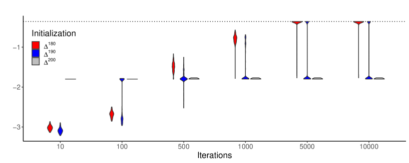
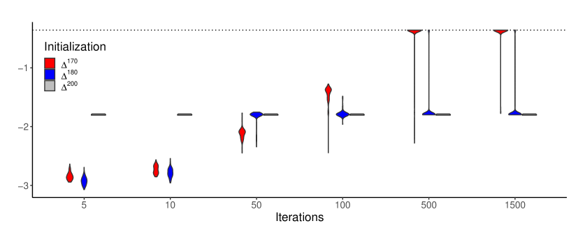
Figure 2: Violin plots visualizing MCMC trajectories for one simulated data set. Each violin gives the distribution of the log-posterior probability (scaled by $10^{-3}$) of the sampled model across 100 runs. The top panel is for the random walk MH algorithm, and the lower is for the informed MH algorithm. Algorithms are initialized at models uniformly sampled from $\Delta^{m}$, and each color represents one choice of $m$. The black dotted line indicates the scaled log-posterior probability of the true model.

	RWMH	IMH	IMH-unclipped
Success	100	100	0
$H_{\mathrm{true}}$	1811	27	–
Time	13.6	9.3	35.3
$T_{\mathrm{true}}$	9.1	7.5	–

Table 4: Results for 100 replicates with moderately correlated design. Each algorithm is initialized at $\delta$ uniformly sampled from $\Delta^{20}$.

6.1.2 Highly correlated design

When the design matrix exhibits a high degree of collinearity, we expect that $\pi$ can be highly multimodal, and local modes may occur on $(\mathcal{V}_{s},\mathcal{N}_{1})$ even for small $s$. Hence, unlike in the moderately correlated setting where we only need to initialize the sampler at a sufficiently sparse model, we may need to impose much stronger assumptions on the initialization so that the samplers can quickly find the true model.

To investigate this, we generate 100 replicates of $(\bm{X},\bm{y})$ under the highly correlated setting, and consider two initialization schemes studied in Atchadé (2021). We denote them by $\delta^{\mathrm{bad}}$ and $\delta^{\mathrm{good}}$. Both $\delta^{\mathrm{bad}}$ and $\delta^{\mathrm{good}}$ include 50 randomly sampled variables that are not in $\delta^{*}$ (i.e., false positives), and for each $j\in[5]$, $\delta^{\mathrm{good}}_{j}=1$ while $\delta^{\mathrm{bad}}_{j}=0$. Hence, $\delta^{\mathrm{bad}}$ satisfies $||\delta^{\mathrm{bad}}||_{1}=50$ and has 5 false negatives, and $\delta^{\mathrm{good}}$ satisfies $||\delta^{\mathrm{good}}||_{1}=55$ with no false negative. Table 5 summarizes the results. When started at $\delta^{\mathrm{bad}}$, both samplers fail to find $\delta^{*}$ in most replicates, and IMH is still more sensitive to nearby local modes as in the simulation study with moderately correlated design. When started at $\delta^{\mathrm{good}}$, both algorithms recover $\delta^{*}$ quickly, and IMH has a slightly higher success rate than RWMH. This result suggests that $\pi$ is probably highly multimodal among models with false negatives (recall that in Example 3, the posterior probability can decrease when we add some variable that is in the true model), and the identification of $\delta^{*}$ requires a warm start that already includes $\delta^{*}$ as a submodel.

	RWMH		IMH
Initialization	$\delta^{\mathrm{bad}}$	$\delta^{\mathrm{good}}$	$\delta^{\mathrm{bad}}$	$\delta^{\mathrm{good}}$
Success	27	95	3	100
$H_{\mathrm{true}}$	–	2198	–	51
Time	13.2	13.5	13.1	19.6
$T_{\mathrm{true}}$	–	9.5	–	8.7

Table 5: Results for 100 replicates with highly correlated design. See the main text for how $\delta^{\mathrm{bad}}$ and $\delta^{\mathrm{good}}$ are generated.

6.2 Bayesian Community Detection

Consider the community detection problem with only two communities, where the goal is to estimate the community assignment vector $z\in\{1,2\}^{p}$ from an observed undirected graph represented by a symmetric adjacency matrix $A\in\{0,1\}^{p\times p}$. Here $z_{j}\in\{1,2\}$ denotes the community assignment of the $j$-th node. We construct a posterior distribution by following the model and prior distribution used in Zhuo and Gao (2021) and Legramanti et al. (2022):

$$A_{ij}\mid Q,z\stackrel{{\scriptstyle\text{ind}}}{{\sim}}\mathrm{Bernoulli}(Q_{z_{i}z_{j}}),\;\forall\,i,j\in[p]\text{ and }i<j,$$ (34)

$$Q_{uv}\stackrel{{\scriptstyle\text{iid}}}{{\sim}}\mathrm{Uniform}(0,1),\quad\forall\,u,v\in[p]\text{ and }u\leq v,$$

$$\pi_{0}(z)\propto 1,\quad\forall\,z\in\{1,2\}^{p},$$

where $\pi_{0}(z)$ denotes the prior distribution of $z$ and $Q_{uv}$ is the edge connection probability between one node from community $u$ and another from community $v$. By integrating out $Q$, we obtain a posterior distribution $\pi$ on the finite space $\{1,2\}^{p}$. Note that due to label switching, we have $\pi(z)=\pi(\tilde{z})$, where $\tilde{z}$ is defined by $\tilde{z}_{j}=3-z_{j}$.

In the simulation, we set $p=1,000$ and let the true community assignment vector $z^{*}$ be given by $z^{*}_{j}=1$ if $1\leq j\leq p/2$ and $z^{*}_{j}=2$ otherwise. We generate the observed graph by sampling each $A_{ij}$ (with $i<j$) independently from $\mathrm{Bernoulli}(p_{\mathrm{within}})$ when $z_{i}=z_{j}$ and from $\mathrm{Bernoulli}(p_{\mathrm{between}})$ when $z_{i}\neq z_{j}$. We use $p_{\mathrm{within}}=10^{-1}$ and $p_{\mathrm{between}}=10^{-8}$ so that the two communities are well separated in the observed graph.

We consider both random walk MH (RWMH) and informed MH (IMH) algorithms, whose proposal neighborhood is defined as $\mathcal{N}(z)=\{z^{\prime}:d_{\mathrm{H}}(z,z^{\prime})=1\}$, where $d_{\mathrm{H}}$ is the Hamming distance. In words, the proposal only changes the community assignment of one node. For IMH, this time we use $\ell=p^{-1}$ and $L=p^{3}$ (reason will be explained later). We simulate 100 data sets, and for each data set we run RWMH for 20,000 iterations and IMH for 2,000 iterations. We consider two different initialization schemes, denoted by $z^{\mathrm{bad}}$ and $z^{\mathrm{good}}$. The assignment vector $z^{\mathrm{bad}}$ is randomly generated such that half of the community assignments are incorrect, while $z^{\mathrm{good}}$ is generated with only one third of the assignments being incorrect. We summarize the results in Table 6 where the four metrics are defined similarly to those used in Section 6.1. Note that we treat both $z^{*}$ and $\tilde{z}^{*}$ as the true model, where $\tilde{z}^{*}_{j}=3-z^{*}_{j}$ for each $j\in[p]$.

The result confirms our theoretical findings in Section 5 regarding the effect of initialization on the mixing. When we initialize the samplers at $z^{\mathrm{bad}}$, fewer than 50 % of the runs reach the true assignment vector up to label switching, while all chains find the true assignment within a reasonable number of iterations when $z^{\mathrm{good}}$ is used for initialization. In Figure 3, we plot the scaled log-posterior trajectories of 100 MCMC runs for one simulated data set. The figure shows that some runs initialized at $z^{\mathrm{bad}}$ get trapped near it, and when the chain is initialized at $z^{\mathrm{good}}$, it exhibits much faster mixing.

We have also tried IMH with $\ell=p$ and $L=p^{3}$ and observed that in all 100 replicates with initial state $z^{\mathrm{bad}}$, the sampler fails to find the true assignment vector and gets stuck around $z^{\mathrm{bad}}$. We have numerically examined the posterior landscape around $z^{\mathrm{bad}}$ and found that the ratio $\pi(z^{\prime})/\pi(z^{\mathrm{bad}})$, where $z^{\prime}=\operatorname*{arg\,max}_{z\in\mathcal{N}(z^{\mathrm{bad}})}\pi(z)$, is always very small (often around $1$). Hence, an informed proposal with $\ell=p=1,000$ only proposes $z^{\prime}$ with probability $1/p$ (and may get rejected due to small acceptance rates). For comparison, using $\ell=p^{-1}$ assigns larger proposal probability to $z^{\prime}$ and sometimes does help IMH move away from $z^{\mathrm{bad}}$, as shown in Figure 3.

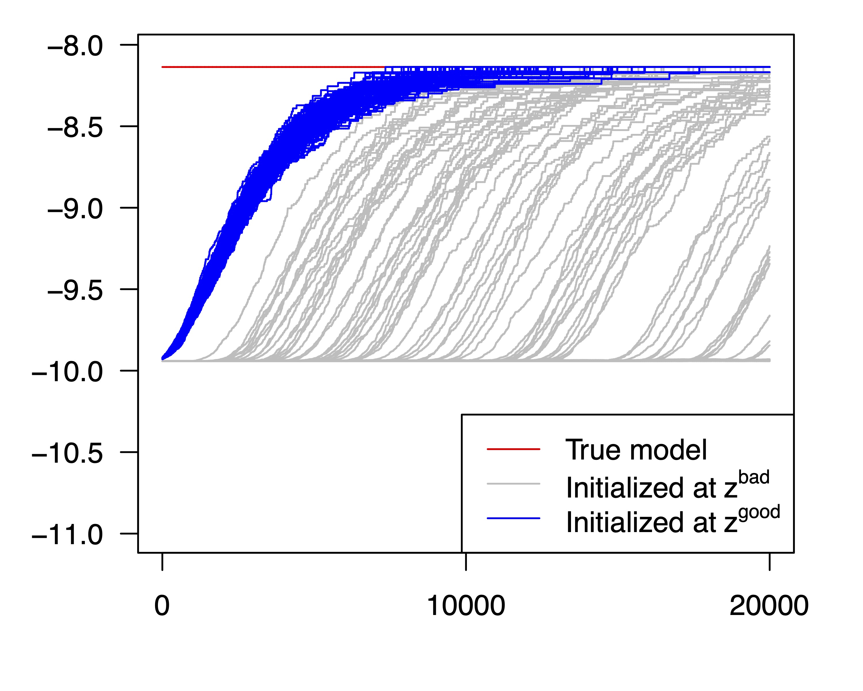
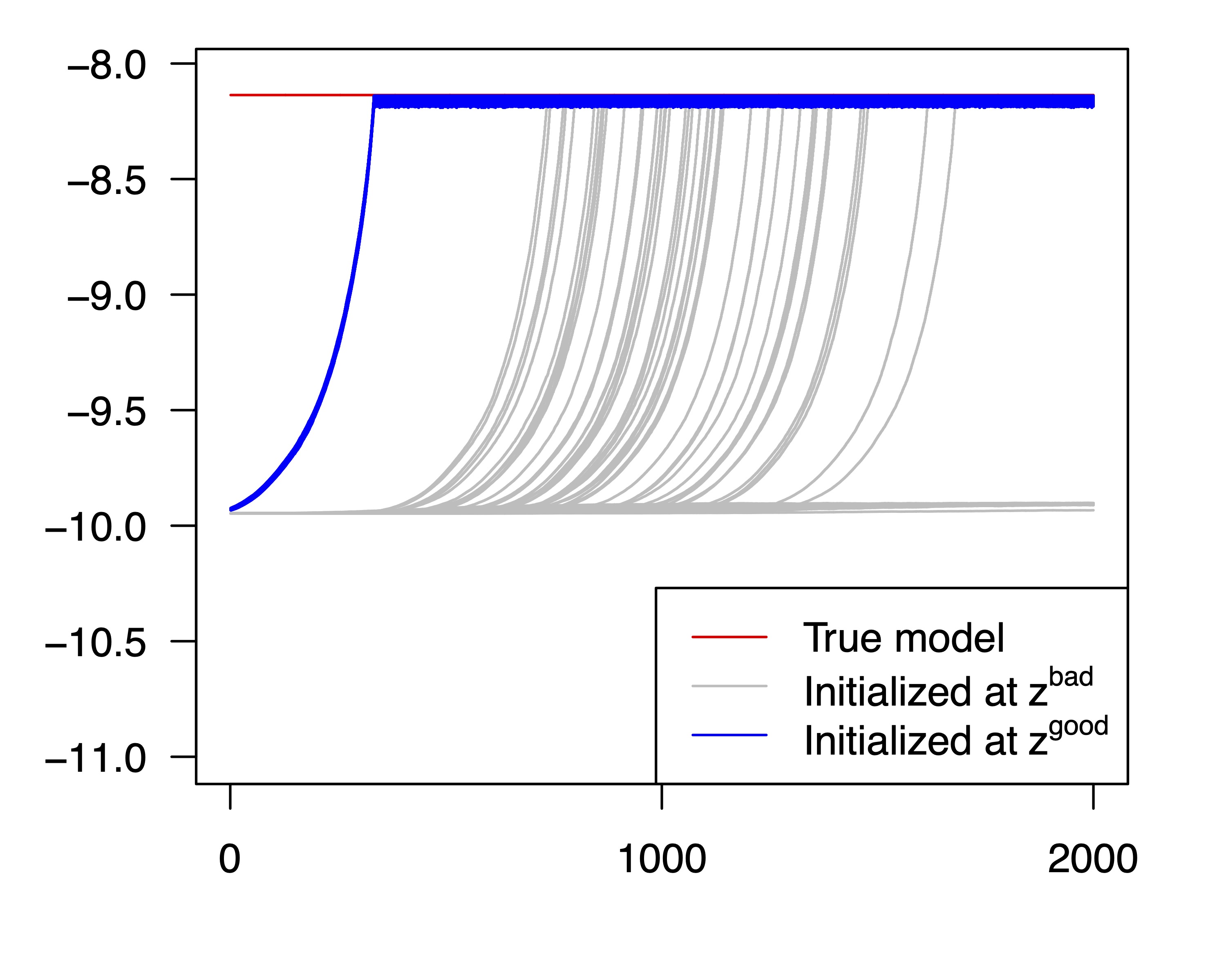
Figure 3: Log-posterior probability $\times 10^{-4}$ versus the number of iterations in 100 MCMC runs, initialized at $z^{\mathrm{bad}}$ (gray) or $z^{\mathrm{good}}$ (blue). The red line indicates the log posterior probability of the true assignment. The left panel is for RWMH, and the right is for IMH.

	RWMH		IMH
Initialization	$z^{\mathrm{bad}}$	$z^{\mathrm{good}}$	$z^{\mathrm{bad}}$	$z^{\mathrm{good}}$
Success	41	100	49	100
$H_{\mathrm{true}}$	–	10901	–	333
Time	8.4	6.8	76.1	75.5
$T_{\mathrm{true}}$	–	5.6	–	13.4

Table 6: Results for 100 replicates of the community detection problem. See the main text for how $z^{\mathrm{bad}}$ and $z^{\mathrm{good}}$ are generated.

7 Discussion and Concluding Remarks

Our theory suggests that an MH algorithm converges fast if it is initialized within a set $\mathcal{X}_{0}$ such that $\pi(\mathcal{X}_{0})$ is large and $\pi$ is unimodal on $\mathcal{X}_{0}$ with respect to the given neighborhood relation $\mathcal{N}$. In practice, it is difficult to determine if $\pi$ is indeed unimodal with respect to $\mathcal{N}$, and thus a larger proposal neighborhood is sometimes preferred to prevent the chain from getting stuck at local modes. For example, in variable selection, one can enlarge the proposal neighborhood by allowing adding or removing multiple variables simultaneously, which is a common practice in the literature (Lamnisos et al., 2009; Guan and Stephens, 2011; Titsias and Yau, 2017; Zhou and Guan, 2019; Liang et al., 2022; Griffin et al., 2021). However, using a too large neighborhood is not desirable either, which is sometimes called the “Goldilocks principle” (Rosenthal, 2011). Our theory suggests that we should try to use the smallest neighborhood that leaves $\pi$ unimodal on $\mathcal{X}_{0}$. Developing diagnostics related to the unimodal condition could be an interesting direction for future work and provide guidance on choosing the neighborhood size in adaptive methods (Griffin et al., 2021; Liang et al., 2022).

One important technical contribution of this work is that we have demonstrated how to use multicommodity flow method and single-element drift condition to derive mixing time bounds in the context of discrete-space statistical models. To our knowledge, both methods have been rarely considered in the literature on high-dimensional Bayesian statistics. For random walk MH algorithms, the canonical path ensemble method may already provide a nearly optimal spectral gap bound, but for informed MH algorithms, the use of multicommodity flow is crucial to obtaining the dimension-free estimate of the relaxation time. Regarding the drift condition analysis, general theoretical results have been obtained for random walk or gradient-based MH algorithms on Euclidean spaces. In particular, the drift function $V(x)=\pi(x)^{-1/2}$ ($\pi$ denotes the Lebesgue density) has been used to prove geometric ergodicity (Roberts and Tweedie, 1996; Jarner and Hansen, 2000) and to derive explicit convergence rate bounds in the recent work of Bhattacharya and Jones (2023). This choice of $V$ is conceptually similar to the one we introduce in (27), $V(x)=\pi(x)^{1/\log\pi_{\mathrm{min}}}$, where the exponent is chosen deliberately to optimize the mixing time bound. It would be interesting to investigate whether one can also improve the mixing time estimates on Euclidean spaces by using a different exponent (though our choice will not be applicable since $\pi_{\mathrm{min}}$ becomes zero on unbounded spaces).

Both our theory and simulation studies suggest that informed MH algorithms require stronger assumptions on the posterior distribution or initialization scheme to achieve fast mixing. An open question is whether informed samplers still have theoretical guarantees under the regime $M<R<M^{2}$, which is not covered by our results such as Theorem 2. Note that by Theorem 1, random walk MH algorithms mix rapidly in this case.

Finally, we point out that MH sampling schemes may not be the most efficient way to utilize informed proposals. The informed importance tempering algorithm proposed in Zhou and Smith (2022) and Li et al. (2023), which generalizes the tempered Gibbs sampler of Zanella and Roberts (2019), allows one to always accept informed proposals and use importance weighting to correct for the bias. It was shown in Li et al. (2023) that this technique can also be applied to multiple-try Metropolis algorithms (Liu et al., 2000; Chang et al., 2022; Gagnon et al., 2023), making them rejection-free. These multiple-try methods enable the calculation of an informed proposal only on a random subset of $\mathcal{N}(x)$, with the subset’s size adjustable according to available computing resources, which makes them highly flexible and easily applicable to general state spaces.

Appendix A Review of Path Methods

A.1 Spectral Gap and Path Methods

Let $\mathsf{P}\in[0,1]^{|\mathcal{X}|\times|\mathcal{X}|}$ denote the transition probability matrix of an irreducible, aperiodic and reversible Markov chain on the finite state space $\mathcal{X}$. Let $\pi$ denote the stationary distribution and define $\pi(f)=\sum_{x}\pi(x)f(x)$ for any $f\colon\mathcal{X}\rightarrow\mathbb{R}$. Recall that we define the spectral gap of $\mathsf{P}$ as

$$\mathrm{Gap}(\mathsf{P})=1-\max\{\lambda_{2},|\lambda_{|\mathcal{X}|-1}|\},$$

and the relation between spectral gap and mixing time is described by the inequality (11). In words, if $\mathrm{Gap}(\mathsf{P})$ is close to zero, the chain requires a large number of steps to get close to the stationary distribution in total variation distance. Path methods are a class of techniques for finding bounds on $\mathrm{Gap}(\mathsf{P})$ by examining likely trajectories of the Markov chain. They are based on the following variational definition of $\mathrm{Gap}(\mathsf{P})$ (Levin and Peres, 2017, Lemma 13.6):

$$\mathrm{Gap}(\mathsf{P})=\min_{\begin{subarray}{c}f\colon\mathcal{X}\rightarrow\mathbb{R}\\ \textit{ s.t. }\mathrm{Var}_{\pi}(f)\neq 0\end{subarray}}\frac{\mathcal{E}(f)}{\mathrm{Var}_{\pi}(f)},$$ (35)

where $\mathrm{Var}_{\pi}(f)=\sum_{x\in\mathcal{X}}(f(x)-\pi(f))^{2}\pi(x)$, and $\mathcal{E}$ is the Dirichlet form associated to the pair $(\mathsf{P},\pi)$, defined as

$$\mathcal{E}(f)=\langle(\mathsf{I}-\mathsf{P})f,f\rangle_{\pi},$$ (36)

where the inner product is defined by

$$\langle f_{1},f_{2}\rangle_{\pi}=\sum_{x\in\mathcal{X}}f_{1}(x)f_{2}(x)\pi(x).$$

We have the following equivalent characterizations of $\mathcal{E}(f)$ and $\mathrm{Var}_{\pi}(f)$ (Levin and Peres, 2017, Lemma 13.6),

$$\mathcal{E}(f)=\frac{1}{2}\sum_{x,x^{\prime}\in\mathcal{X}}|f(x)-f(x^{\prime})|^{2}\mathsf{P}(x,x^{\prime})\pi(x),$$ (37)

$$\mathrm{Var}_{\pi}(f)=\frac{1}{2}\sum_{x,x^{\prime}\in\mathcal{X}}|f(x)-f(x^{\prime})|^{2}\pi(x)\pi(x^{\prime}).$$ (38)

Given a sequence $\gamma=(x_{0}=x,x_{1},\dots,x_{k-1},x_{k}=x^{\prime})$, we write $e\in\gamma$ with $e=(x_{j-1},x_{j})$ for $j=1,\dots,k$, and we say $e$ is an edge of $\gamma$. We say $\gamma$ is a path if $\gamma$ does not contain duplicate edges. Let $\bar{E}$ be the edge set for $\mathsf{P}$, which is defined by

$$\bar{E}=\{(x,x^{\prime})\in\mathcal{X}^{2}\colon x\neq x^{\prime},\mathsf{P}(x,x^{\prime})>0\}.$$ (39)

Given $E\subset\bar{E}$, let

$$\Gamma_{E}(x,x^{\prime})=\{\text{paths from $x$ to $x^{\prime}$ with all edges in $E$}\},$$ (40)

and let $\Gamma_{E}=\cup_{x\neq x^{\prime}}\Gamma_{E}(x,x^{\prime})$. Define $Q\colon\bar{E}\rightarrow(0,\infty)$ by

$$Q(e)=\pi(x)\mathsf{P}(x,x^{\prime}),\text{ if }e=(x,x^{\prime}).$$ (41)

We now present Proposition 1, which provides a bound on the spectral gap using paths and generalizes the multicommodity flow method of Sinclair (1992).

Proposition 1 (Theorem 3.2.9 in Giné et al. (1996)).

Let $E\subset\bar{E}$, $w\colon E\rightarrow(0,\infty)$, and for $\gamma\in\Gamma_{E}$, define its $w$-length by

$$|\gamma|_{w}=\sum_{e\in\gamma}w(e).$$ (42)

Let a function $\phi\colon\Gamma_{E}\rightarrow[0,\infty)$ satisfy that

$$\sum_{\gamma\in\Gamma_{E}(x,x^{\prime})}\phi(\gamma)=\pi(x)\pi(x^{\prime}),\quad\text{ for any }x\neq x^{\prime}.$$ (43)

Then $\mathrm{Gap}(\mathsf{P})\geq 1/A(E,w,\phi)$, where

$$A(E,w,\phi)=\max_{e\in E}\left\{\frac{\sum_{\gamma\in\Gamma_{E}\colon e\in\gamma}|\gamma|_{w}\phi(\gamma)}{Q(e)w(e)}\right\}.$$ (44)

In Proposition 1, $w$ is called a weight function, and $\phi$ is called a flow function. Proposition 1 directly follows from (37),  (38) and the following lemma, which will be used later for proving a similar result for restricted spectral gap in Section B (see Proposition 2).

Lemma 2.

Let $E\subset\bar{E}$, $w\colon E\rightarrow(0,\infty)$ and $\phi\colon\Gamma_{E}\rightarrow[0,\infty)$. For any $f\colon\mathcal{X}\rightarrow\mathbb{R}$, we have

$$\sum_{x,x^{\prime}\in\mathcal{X}}|f(x^{\prime})-f(x)|^{2}\Phi(x,x^{\prime})\leq\;A(E,w,\phi)\sum_{(x,x^{\prime})\in E}Q((x,x^{\prime}))|f(x^{\prime})-f(x)|^{2},$$

where $A(E,w,\phi)$ is given by (44) and

$$\Phi(x,x^{\prime})=\begin{cases}\sum_{\gamma\in\Gamma_{E}(x,x^{\prime})}\phi(\gamma),&\text{ if }\,\Gamma_{E}(x,x^{\prime})\neq\emptyset,\\ 0,&\text{ otherwise}.\end{cases}$$

Proof.

Given $e=(z,z^{\prime})$, let $\mathrm{d}f(e)=f(z^{\prime})-f(z)$ denote the increment of $f$ along $e$. For any $\gamma\in\Gamma_{E}(x,x^{\prime})$, we can write

$$|f(x^{\prime})-f(x)|^{2}=\sum_{e\in\gamma}\mathrm{d}f(e)=\sum_{e\in\gamma}\sqrt{w(e)}\frac{\mathrm{d}f(e)}{\sqrt{w(e)}}.$$

By the Cauchy-Schwarz inequality,

$$|f(x^{\prime})-f(x)|^{2}\leq|\gamma|_{w}\sum_{e\in\gamma}\frac{(\mathrm{d}f(e))^{2}}{w(e)}.$$

Hence,

$$\sum_{\gamma\in\Gamma_{E}(x,x^{\prime})}\phi(\gamma)|\gamma|_{w}\sum_{e\in\gamma}\frac{(\mathrm{d}f(e))^{2}}{w(e)}\geq|f(x^{\prime})-f(x)|^{2}\Phi(x,x^{\prime}).$$

We sum over $x,x^{\prime}\in\mathcal{X}$, which yields

$$\sum_{x,x^{\prime}\in\mathcal{X}}|f(x^{\prime})-f(x)|^{2}\Phi(x,x^{\prime})\leq\; \sum_{\gamma\in\Gamma_{E}}\phi(\gamma)|\gamma|_{w}\sum_{e\in\gamma}\frac{(\mathrm{d}f(e))^{2}}{w(e)}$$

$$=\; \sum_{e\in E}\frac{(\mathrm{d}f(e))^{2}}{w(e)}\sum_{\begin{subarray}{c}\gamma\,:\,\gamma\in\Gamma_{E}\\ \textit{ s.t. }e\in\gamma\end{subarray}}|\gamma|_{w}\phi(\gamma)$$

$$=\; \sum_{e\in E}\left\{\frac{1}{Q(e)w(e)}\sum_{\begin{subarray}{c}\gamma\,:\,\gamma\in\Gamma_{E}\\ \textit{ s.t. }e\in\gamma\end{subarray}}|\gamma|_{w}\phi(\gamma)\right\}Q(e)(\mathrm{d}f(e))^{2}$$

$$\leq\; A(E,w,\phi)\sum_{e\in E}Q(e)(\mathrm{d}f(e))^{2},$$

which completes the proof. ∎

Remark 8.

Observe that in Lemma 2, one can replace $Q$ with any function that maps from $E$ to $(0,\infty)$. The conclusion still holds and the proof is identical.

Proof of Proposition 1.

By (38),

$$\sum_{x,x^{\prime}\in\mathcal{X}}|f(x^{\prime})-f(x)|^{2}\Phi(x,x^{\prime})=2\mathrm{Var}_{\pi}(f),$$

and by (37),

$$\sum_{(x,x^{\prime})\in E}Q((x,x^{\prime}))|f(x^{\prime})-f(x)|^{2}\leq 2\mathcal{E}(f).$$

The result then follows from (35). ∎

A.2 Review of the Mixing Time Bound in Zhou and Chang (2023)

In this section, we review the proof techniques used in Zhou and Chang (2023) to derive the mixing time bound under the unimodal condition. Similar arguments will be used later in Section B.3 for proving some results of this work. Let the triple $(\mathcal{X},\mathcal{N},\pi)$ satisfy $R(\mathcal{X},\mathcal{N},\pi)>M(\mathcal{X},\mathcal{N}),$ where $R$ and $M$ are defined in (12) and (8) respectively, and recall that we always assume

$$\mathcal{N}(x)=\{x^{\prime}\in\mathcal{X}\colon\mathsf{P}(x,x^{\prime})>0\}.$$

We begin by constructing the functions $\phi$ and $w$ for utilizing Proposition 1.

A.2.1 Constructing a flow $\phi$

Assume that $\pi$ is unimodal on $(\mathcal{X},\mathcal{N})$. We first present a general method for constructing flows by identifying likely paths leading to $x^{*}=\arg\max_{x\in\mathcal{X}}\pi(x)$, and derive a simple upper bound on the maximum load of any edge. For this result, we only need to require $R(\mathcal{X},\mathcal{N},\pi)>1$.

Lemma 3 (Lemma B2 of Zhou and Chang (2023)).

Suppose $(\mathcal{X},\mathcal{N},\pi)$ satisfies $R=R(\mathcal{X},\mathcal{N},\pi)>1$. Let $S\in(1,R]$. Define

$$\mathcal{N}_{S}(x)=\left\{x^{\prime}\in\mathcal{N}(x):\pi(x^{\prime})/\pi(x)\geq S\right\},$$ (45)

and let

$$E_{S}=\{(x,x^{\prime})\colon x\in\mathcal{N}_{S}(x^{\prime})\text{ or }x^{\prime}\in\mathcal{N}_{S}(x)\}$$ (46)

be the resulting edge set. Write $\Gamma_{S}=\Gamma_{E_{S}}$. There exists a flow $\phi\colon\Gamma_{S}\rightarrow[0,\infty)$ such that for any $x\neq x^{\prime}$,

$$\sum_{\gamma\in\Gamma_{S}(x,x^{\prime})}\phi(\gamma)=\pi(x)\pi(x^{\prime}),$$ (47)

and for any $x\neq x^{\prime}$ and $(z,z^{\prime})\in E_{S}$ with $z^{\prime}\in\mathcal{N}_{S}(z)$,

$$\sum_{\begin{subarray}{c}\gamma\colon\gamma\in\Gamma_{S}(x,x^{\prime})\\ \text{ s.t. }(z,z^{\prime})\in\gamma\end{subarray}}\phi(\gamma)\leq\frac{\mathsf{P}(z,\,z^{\prime})}{\mathsf{P}(z,\,\mathcal{N}_{S}(z))}\pi(x)\pi(x^{\prime}).$$ (48)

Proof.

Define an auxiliary transition matrix $\mathsf{P}_{S}$ on $\mathcal{X}\times\mathcal{X}$ by

$$\mathsf{P}_{S}(x,x^{\prime})= \begin{cases}\frac{\mathsf{P}(x,\,x^{\prime})}{\mathsf{P}(x,\,\mathcal{N}_{S}(x))}\mathbbm{1}_{\mathcal{N}_{S}(x)}(x^{\prime}),&\text{if }\mathcal{N}_{S}(x)\neq\emptyset,\vspace{0.2cm}\\ 0,&\text{if }\mathcal{N}_{S}(x)=\emptyset,\vspace{0.2cm}\\ 1-\sum_{\tilde{x}\neq x}\mathsf{P}_{S}(x,\tilde{x}),&\text{if }x=x^{\prime}.\end{cases}$$ (49)

Given $\gamma=\left(x_{0},x_{1},\ldots,x_{k}\right)$, let $\stackrel{{\scriptstyle\leftarrow}}{{\gamma}}=(x_{k},x_{k-1},\dots,x_{0})$ be the reversed path of $\gamma$. We first construct a normalized flow function, denoted by $f^{S}:\Gamma_{S}\rightarrow[0,1]$, as follows.

1. If $x^{*}$ does not occur in $\gamma$ or $x^{*}$ occurs at least twice in $\gamma$, let $f^{S}(\gamma)=0$.

2. If $x_{k}=x^{*}$, let $f^{S}(\gamma)=\prod_{i=1}^{k}\mathsf{P}_{S}\left(x_{i-1},x_{i}\right)$.

3. If $x_{0}=x^{*}$, let $f^{S}(\gamma)=f^{S}(\stackrel{{\scriptstyle\leftarrow}}{{\gamma}})$.

4. Define $f^{S}(\gamma)=f^{S}\left(\gamma_{1}\right)f^{S}\left(\gamma_{2}\right)$ if $x_{j}=x^{*}$ for some $1\leq j\leq k-1$, where $\gamma_{1}=\left(x_{0},\ldots,x_{j-1},x^{*}\right)$ and $\gamma_{2}=\left(x^{*},x_{j+1},\ldots,x_{k}\right)$.

Then, the following properties hold for $f^{S}$ by Lemma B2 in Zhou and Chang (2023). For any $x,x^{\prime}\in\mathcal{X}$ with $x\neq x^{\prime}$, we have

$$\sum_{\gamma\in\Gamma_{S}(x,x^{\prime})}f^{S}(\gamma)=1,$$ (50)

and for $e=(z,z^{\prime})$ with $z^{\prime}\in\mathcal{N}_{S}(z)$,

$$\sum_{\begin{subarray}{c}\gamma\colon\gamma\in\Gamma_{S}(x,x^{\prime})\\ \textit{ s.t. }e=(z,z^{\prime})\in\gamma\end{subarray}}f^{S}(\gamma)\leq\mathsf{P}_{S}(z,z^{\prime}).$$ (51)

The flow $\phi$ is then obtained by

$$\phi(\gamma)=f^{S}(\gamma)\pi(x)\pi(x^{\prime}),\text{ if }\gamma\in\Gamma_{S}(x,x^{\prime}),$$ (52)

which satisfies (43) and (48). ∎

Remark 9.

This result can be generalized by replacing $\mathcal{N}_{S}$ with any $\tilde{\mathcal{N}}$ such that

1. $\tilde{\mathcal{N}}(x)\neq\emptyset$ for any $x\neq x^{*}$,

2. $\pi(y)>\pi(x)$ whenever $y\in\tilde{\mathcal{N}}(x)$.

One can then define a transition matrix $\tilde{\mathsf{P}}$ analogously to $\mathsf{P}_{S}$, which is a Markov chain with absorbing state $x^{*}$. The same argument then completes the proof.

A.2.2 Defining a weight function $w$

Consider $E_{S}$ defined in Lemma 3. For $e=(z,z^{\prime})\in E_{S}$ such that $z^{\prime}\in\mathcal{N}_{S}(z)$, we define

$$w(e)=w(\stackrel{{\scriptstyle\leftarrow}}{{e}})=\pi(z)^{-q},$$ (53)

where $q\in(0,1)$ is a constant and $\stackrel{{\scriptstyle\leftarrow}}{{e}}=(z^{\prime},z)$. Let $\Gamma_{S}$ be as defined in Lemma 3 with $S>1$. For any $\gamma\in\Gamma_{S}(x,x^{\prime})$ with $\phi(\gamma)>0$, we have

$$|\gamma|_{w}\leq\frac{\pi(x)^{-q}+\pi(x^{\prime})^{-q}}{1-S^{-q}}.$$ (54)

To obtain (54), we first decompose $\gamma$ to two sub-paths $\gamma_{1},\gamma_{2}$ such that $\gamma_{1}\in\Gamma(x,x^{*})$ and $\gamma_{2}\in\Gamma(x^{*},x^{\prime})$, which exists by our construction of $\phi$. Letting $\gamma_{1}=(x=x_{0},x_{1},\dots,x_{k}=x^{*})$, we obtain by the geometric series calculation that

$$|\gamma_{1}|_{w}=\sum_{j=0}^{k-1}\pi(x_{j})^{-q}\leq\sum_{j=0}^{k-1}\pi(x)^{-q}S^{-q}\leq\frac{\pi(x)^{-q}}{1-S^{-q}}.$$

Calculating $|\gamma_{2}|_{w}$ in the same manner and using $|\gamma|_{w}=|\gamma_{1}|_{w}+|\gamma_{2}|_{w}$, we get (54).

A.2.3 Spectral gap bound

Using $\phi$ and $w$ constructed above, we can now derive a spectral gap bound.

Lemma 4.

Suppose the triple $(\mathcal{X},\mathcal{N},\pi)$ satisfies

$$R=R(\mathcal{X},\mathcal{N},\pi)>M(\mathcal{X},\mathcal{N})=M,$$

and let $x^{*}=\operatorname*{arg\,max}_{x\in\mathcal{X}}\pi(x)$. Let $E_{S},\phi$ be as given in Lemma 3 with $S\in(M,R]$ and $w$ be given by (53). Then,

$$A(E_{S},w,\phi)\leq\frac{c(S/M)}{2}\max_{z\in\mathcal{X}\setminus\{x^{*}\}}\frac{1}{\mathsf{P}(z,\mathcal{N}_{S}(z))},$$ (55)

where $A$ is given by (44) and $c(u)=4(1-u^{-1/2})^{-3}.$

Proof.

We first fix $e=(z,z^{\prime})\in E_{S}$ with $z^{\prime}\in\mathcal{N}_{S}(z)$. The case with $z\in\mathcal{N}_{S}(z^{\prime})$ can be analyzed in the same manner by symmetry. Observe that

$$\frac{1}{Q(e)w(e)}\sum_{\begin{subarray}{c}\gamma\colon\gamma\in\Gamma_{S}\\ \textit{s.t. }e\in\gamma\end{subarray}}\phi(\gamma)|\gamma|_{w}=\;\frac{1}{Q(e)w(e)}\sum_{x\neq x^{\prime}}\sum_{\begin{subarray}{c}\gamma\colon\gamma\in\Gamma_{S}(x,x^{\prime})\\ \textit{s.t. }e\in\gamma\end{subarray}}\phi(\gamma)|\gamma|_{w}.$$

For fixed $x,x^{\prime}\in\mathcal{X}$ with $x\neq x^{\prime}$,

$$\frac{1}{Q(e)w(e)}\sum_{\begin{subarray}{c}\gamma\colon\gamma\in\Gamma_{S}(x,x^{\prime})\\ \textit{s.t. }e\in\gamma\end{subarray}}\phi(\gamma)|\gamma|_{w}\leq\; \frac{\pi(x)^{-q}+\pi(x^{\prime})^{-q}}{\pi(z)^{1-q}(1-S^{-q})\mathsf{P}(z,z^{\prime})}\sum_{\begin{subarray}{c}\gamma\colon\gamma\in\Gamma_{S}(x,x^{\prime})\\ \textit{ s.t. }e\in\gamma\end{subarray}}\phi(\gamma)$$

$$\leq\; \frac{\pi(x)^{1-q}\pi(x^{\prime})+\pi(x)\pi(x^{\prime})^{1-q}}{\pi(z)^{1-q}(1-S^{-q})}\frac{1}{\mathsf{P}(z,\mathcal{N}_{S}(z))},$$

where the first inequality is from (54) and the last inequality is due to (48) with the definition in (49).

Let $\Lambda(z)=\{x\colon\pi(x)<\pi(z),\;\exists\gamma\in\Gamma_{S}(z,x)\text{ s.t. }\phi(\gamma)>0\}\cup\{z\}$ denote the set of ancestors of $z$ in the graph $(X,E_{S})$ (each edge is directed towards the state with larger posterior probability). Note that

$$\sum_{\gamma\in\Gamma_{S}(x,x^{\prime})\colon e\in\gamma}\phi(\gamma)>0$$

only if $x$ or $x^{\prime}$ belongs to $\Lambda(z)$. Hence, summing over distinct $(x,x^{\prime})$ and using $\pi(x)\leq 1$ for any $x$, we get

$$\frac{1}{Q(e)w(e)}\sum_{\begin{subarray}{c}\gamma\colon\gamma\in\Gamma_{S}\\ \textit{s.t. }e\in\gamma\end{subarray}}\phi(\gamma)|\gamma|_{w}\leq\; \sum_{x\in\Lambda(z)}\sum_{x^{\prime}\in\mathcal{X}}\frac{2\pi(x)^{1-q}\pi(x^{\prime})^{1-q}}{\pi(z)^{1-q}(1-S^{-q})}\frac{1}{\mathsf{P}(z,\mathcal{N}_{S}(z))}.$$

Using $S>M$, a routine geometric series calculation gives

$$\sum_{x\in\Lambda(z)}\sum_{x^{\prime}\in\mathcal{X}}\pi(x)^{1-q}\pi(x^{\prime})^{1-q}\leq\frac{\pi(z)^{1-q}}{(1-MS^{-(1-q)})^{2}}.$$

(See also Lemma 3 of Zhou and Smith (2022).) Finally, set $q=\log(S/M)/(2\log S)$ so that $S^{-q}=MS^{-(1-q)}$; note that $q\in(0,1)$ since $S>M\geq 1$. We then obtain the asserted result by taking maximum over $e\in E_{S}$. ∎

Appendix B Path Methods for Restricted Spectral Gaps

B.1 Restricted Spectral Gap

If there are isolated local modes, the spectral gap of the Markov chain can be extremely close to 0. This remains true even when all local modes (other than the global one) have negligible probability mass are highly unlikely to be visited by the chain if it is properly initialized. As a result, calculating the standard spectral gap bound yields an overly conservative estimate of the mixing time. To address this issue, we work with the restricted spectral gap, which was considered in Atchadé (2021).

We still use the notation introduced in Appendix A. Given a function $f\colon\mathcal{X}\rightarrow\mathbb{R}$, let

$$||f||_{L^{m}(\pi)}=\left(\sum_{x\in\mathcal{X}}|f(x)|^{m}\pi(x)\right)^{1/m},\text{ for }m\in(2,\infty].$$ (56)

Given $\mathcal{X}_{0}\subset\mathcal{X}$, define the $\mathcal{X}_{0}$-restricted spectral gap by

$$\mathrm{Gap}_{\mathcal{X}_{0}}(\mathsf{P})= \inf_{f\colon\mathrm{Var}_{\pi}(f)>0}\frac{\sum_{x,y\in\mathcal{X}_{0}}(f(x)-f(y))^{2}\mathsf{P}(x,y)\pi(x)}{\sum_{x,y\in\mathcal{X}_{0}}(f(x)-f(y))^{2}\pi(x)\pi(y)}.$$ (57)

We note that if $\mathcal{X}_{0}=\mathcal{X}$, $\mathrm{Gap}_{\mathcal{X}_{0}}(\mathsf{P})$ coincides with $\mathrm{Gap}(\mathsf{P})$. The following lemma is from Atchadé (2021), which shows that we can use restricted spectral gap to bound the mixing time given a sufficiently good initial distribution.

Lemma 5.

Let $\epsilon\in(0,1/2)$ and $\pi_{0}$ be another distribution on $\mathcal{X}$. Define $f_{0}=\pi_{0}/\pi$. Choose any $m\in(2,\infty]$, and let $B\in[1,\infty)$ be such that $||f_{0}||_{L^{m}(\pi)}\leq B$. If $\mathcal{X}_{0}\subset\mathcal{X}$ satisfies

$$\pi(\mathcal{X}_{0})\geq 1-\left(\frac{\epsilon^{2}}{5B^{2}}\right)^{1+\frac{2}{m-2}},$$

then $||\pi_{0}P^{t}-\pi||_{\rm{TV}}\leq\epsilon$ for any $t$ such that

$$t\geq\frac{\log(B^{2}/2\epsilon^{2})}{\mathrm{Gap}_{\mathcal{X}_{0}}(\mathsf{P})}.$$

Proof.

This follows from Lemma 1 and Lemma 2 of Atchadé (2021) and the argument after Lemma 2 in Atchadé (2021). Note that Atchadé (2021) used a different scaling in the definition of the total variation distance. ∎

B.2 Multicommodity Flow Bounds

Given a subset $\mathcal{X}_{0}\subseteq\mathcal{X}$, recall that we write

$$\mathcal{N}|_{\mathcal{X}_{0}}(x)=\{x^{\prime}\in\mathcal{X}_{0}\colon\mathsf{P}(x,x^{\prime})>0\},$$ (58)

for each $x\in\mathcal{X}_{0}$. Similarly, let

$$\bar{E}_{0}=\left\{(x,x^{\prime})\in\mathcal{X}_{0}^{2}\colon x\neq x^{\prime}\text{ and }\mathsf{P}(x,x^{\prime})>0\right\}$$ (59)

denote the edge set of $\mathsf{P}$ restricted to $\mathcal{X}_{0}$. Given $E_{0}\subset\bar{E}_{0}$, let $\Gamma_{0}(x,x^{\prime})=\Gamma_{E_{0}}(x,x^{\prime})$ and $\Gamma_{0}=\Gamma_{E_{0}}$ denote the corresponding path sets. We provide the following proposition that extends the argument used in Proposition 1 to the restricted spectral gap.

Proposition 2.

Let $E_{0}\subset\bar{E}_{0}$, $w\colon E_{0}\rightarrow(0,\infty)$, and for $\gamma\in\Gamma_{0}$, define $|\gamma|_{w}$ as in (42). Let $\phi\colon\Gamma_{0}\rightarrow[0,\infty)$ satisfy that

$$\sum_{\gamma\in\Gamma_{0}(x,x^{\prime})}\phi(\gamma)=\pi(x)\pi(x^{\prime}),\;\forall x,x^{\prime}\in\mathcal{X}_{0},\;x\neq x^{\prime}.$$ (60)

Then $\mathrm{Gap}_{\mathcal{X}_{0}}(\mathsf{P})\geq 1/A(E_{0},w,\phi)$, where $A$ is defined by (44).

Proof.

By Lemma 2, for any $f\colon\mathcal{X}\rightarrow\mathbb{R}$,

$$\sum_{x,x^{\prime}\in\mathcal{X}}|f(x^{\prime})-f(x)|^{2}\Phi(x,x^{\prime})\leq\; A(E_{0},w,\phi)\sum_{(x,x^{\prime})\in E_{0}}Q((x,x^{\prime}))|f(x^{\prime})-f(x)|^{2},$$

where $\Phi(x,x^{\prime})=\sum_{\gamma\in\Gamma_{E}(x,x^{\prime})}\phi(\gamma)$. If $x\notin\mathcal{X}_{0}$ or $x^{\prime}\notin\mathcal{X}_{0}$, $\Gamma_{0}(x,x^{\prime})=\emptyset$ and thus $\Phi(x,x^{\prime})=0$. Hence,

$$\sum_{x,x^{\prime}\in\mathcal{X}}|f(x)-f(x^{\prime})|^{2}\Phi(x,x^{\prime})=\; \sum_{x,x^{\prime}\in\mathcal{X}_{0}}|f(x)-f(x^{\prime})|^{2}\Phi(x,x^{\prime})$$

$$=\; \sum_{x,x^{\prime}\in\mathcal{X}_{0}}|f(x)-f(x^{\prime})|^{2}\pi(x)\pi(x^{\prime}).$$

Further, since $E_{0}\subset\mathcal{X}_{0}^{2}$,

$$\sum_{(x,x^{\prime})\in E_{0}}Q((x,x^{\prime}))|f(x)-f(x^{\prime})|^{2}\leq\sum_{x,x^{\prime}\in\mathcal{X}_{0}}|f(x)-f(x^{\prime})|^{2}\mathsf{P}(x,x^{\prime})\pi(x).$$

The result then follows from the definition of the restricted spectral gap $\mathrm{Gap}_{\mathcal{X}_{0}}(\mathsf{P})$. ∎

B.3 Application of the Multicommodity Flow Method under the Restricted Unimodal Condition

In this section, we assume $R|_{\mathcal{X}_{0}}>M$ and show that the multicommodity flow method reviewed in Section A.2 is also applicable to bounding the restricted spectral gap. For $S\in(M,R|_{\mathcal{X}_{0}}]$, we define

$$\quad\mathcal{N}|_{\mathcal{X}_{0}}^{S}(x)=\left\{x^{\prime}\in\mathcal{N}|_{\mathcal{X}_{0}}(x):\pi(x^{\prime})/\pi(x)\geq S\right\},$$ (61)

and

$$E_{S}^{0}=\{(x,x^{\prime}):x\in\mathcal{N}|^{S}_{\mathcal{X}_{0}}(x^{\prime})\text{ or }x^{\prime}\in\mathcal{N}|^{S}_{\mathcal{X}_{0}}(x)\}.$$ (62)

Let $\Gamma_{S}^{0}=\Gamma_{E_{S}^{0}}$ denote the resulting path set.

Lemma 6.

Suppose the triple $(\mathcal{X}_{0},\mathcal{N}|_{\mathcal{X}_{0}},\pi)$ satisfies

$$R|_{\mathcal{X}_{0}}=R(\mathcal{X}_{0},\mathcal{N}|_{\mathcal{X}_{0}},\pi)>M(\mathcal{X},\mathcal{N})=M,$$

and let $x^{*}_{0}=\operatorname*{arg\,max}_{x\in\mathcal{X}_{0}}\pi(x)$. Let $E_{S}^{0}$ be given by (62) with $S\in(M,R|_{\mathcal{X}_{0}}]$. Then, there exist $w\colon E_{S}^{0}\rightarrow(0,\infty)$, $\phi\colon\Gamma_{S}^{0}\rightarrow[0,\infty)$ such that $\phi$ satisfies (60) and

$$A(E_{S}^{0},w,\phi)\leq\frac{c(S/M)}{2}\max_{z\in\mathcal{X}_{0}\setminus\{x^{*}_{0}\}}\frac{1}{\mathsf{P}(z,\mathcal{N}|_{\mathcal{X}_{0}}^{S}(z))},$$ (63)

where $A$ is given by (44) and $c(u)=4(1-u^{-1/2})^{-3}.$

Proof.

Let $\mathsf{P}|_{\mathcal{X}_{0}}$ denote the restriction of $\mathsf{P}$ to $\mathcal{X}_{0}$; that is, $\mathsf{P}|_{\mathcal{X}_{0}}(x,x^{\prime})=\mathsf{P}(x,x^{\prime})$ if $x,x^{\prime}\in\mathcal{X}_{0}$ and $x\neq x^{\prime}$. Apply Lemma 3 to $\mathsf{P}|_{\mathcal{X}_{0}}$ on $(\mathcal{X}_{0},\mathcal{N}|_{\mathcal{X}_{0}})$, which is allowed since $R|_{\mathcal{X}_{0}}>1$. We then obtain a flow $\phi\colon\Gamma_{S}^{0}\rightarrow[0,\infty)$ such that (60) is satisfied and

$$\sum_{\begin{subarray}{c}\gamma\colon\gamma\in\Gamma_{S}^{0}(x,x^{\prime})\\ \textit{s.t. }(z,z^{\prime})\in\gamma\end{subarray}}\phi(\gamma)\leq\; \frac{\mathsf{P}|_{\mathcal{X}_{0}}(z,z^{\prime})}{\mathsf{P}|_{\mathcal{X}_{0}}(z,\,\mathcal{N}|_{\mathcal{X}_{0}}^{S}(z))}\pi(x)\pi(x^{\prime})$$ (64)

$$=\; \frac{\mathsf{P}(z,z^{\prime})}{\mathsf{P}(z,\,\mathcal{N}|_{\mathcal{X}_{0}}^{S}(z))}\pi(x)\pi(x^{\prime})$$ (65)

for any $x,x^{\prime}\in\mathcal{X}_{0}$ with $x\neq x^{\prime}$ and $(z,z^{\prime})\in E_{S}^{0}$ with $z^{\prime}\in\mathcal{N}|_{\mathcal{X}_{0}}^{S}(z)$.

The asserted bound on $A(E_{S}^{0},w,\phi)$ can be derived by repeating the argument used for proving Lemma 4 on the restricted space $(\mathcal{X}_{0},\mathcal{N}|_{\mathcal{X}_{0}})$. Note that the only difference is that $\pi$ is no longer a probability measure on $(\mathcal{X}_{0},\mathcal{N}|_{\mathcal{X}_{0}})$. But this does not affect the proof since the proof of Lemma 4 only relies on $\max_{x}\pi(x)\leq 1$. ∎

Appendix C Review of Single-element Drift Condition

The drift-and-minorization method is one of the most frequently used techniques for deriving the convergence rates of Markov chains on general state spaces. It directly bounds the total variation distance from the stationary distribution without using the spectral gap. For our purpose, we only need to use the single-element drift condition considered in Jerison (2016), which is particularly useful on discrete spaces.

Definition 1 (single-element drift condition).

The transition matrix $\mathsf{P}$ satisfies a single-element drift condition if there exist an element $x^{*}\in\mathcal{X}$, a function $V:\mathcal{X}\rightarrow[1,\infty)$, and constants $0<\alpha<1$ such that $(\mathsf{P}V)(x)\leq\alpha V(x)$ for all $x\in\mathcal{X}\setminus\{x^{*}\}$.

Note that in Jerison (2016), the single-element drift condition is proposed for general-state-space Markov chains, and one needs to further require that $(\mathsf{P}V)(x^{*})<\infty$ (this holds trivially in our case since $\mathcal{X}$ is finite). Given this drift condition, we can bound the mixing time using the following result of Jerison (2016). Recall that we assume $\mathsf{P}$ is reversible and thus its eigenvalues are all real.

Lemma 7 (Theorem 4.5 of Jerison (2016)).

Suppose $\mathsf{P}$ has non-negative eigenvalues and satisfies the single-element drift condition given in Definition 1. Then, for all $t\geq 0,x\in\mathcal{X}$,

$$\left\|\mathsf{P}^{t}(x,\cdot)-\pi\right\|_{\mathrm{TV}}\leq 2V(x)\alpha^{t+1}.$$

Therefore, we have

$$\tau_{x}(\mathsf{P},\epsilon)\leq\frac{1}{1-\alpha}\log\left(\frac{2V(x)}{\epsilon}\right).$$

Proof.

This directly follows from Theorem 4.5 of Jerison (2016) and the inequality $\log\alpha<\alpha-1$ for $\alpha\in(0,1)$ ∎

Appendix D Proofs

Proof of Lemma 1.

Since $Z_{h}(x)\geq L$, we have

$$\mathsf{K}_{h}\left(x,x^{\prime}\right) =\frac{h(\pi(x^{\prime})/\pi(x))}{Z_{h}(x)}\leq\frac{h(\pi(x^{\prime})/\pi(x))}{L},$$

$$\mathsf{K}_{h}\left(x^{\prime},x\right) =\frac{h(\pi(x)/\pi(x^{\prime}))}{Z_{h}(x^{\prime})}\geq\frac{\ell}{ML},$$

where the second equality follows from $h\in[\ell,L]$ and $|\mathcal{N}(x^{\prime})|\leq M$. Combining the two inequalities, we get

$$\frac{\pi\left(x^{\prime}\right)\mathsf{K}_{h}\left(x^{\prime},x\right)}{\pi(x)\mathsf{K}_{h}\left(x,x^{\prime}\right)} \geq\frac{\pi(x^{\prime})/\pi(x)}{h(\pi(x^{\prime})/\pi(x))}\frac{\ell}{M}.$$

Since $\pi(x^{\prime})/\pi(x)\geq\ell$ and $h(u)\leq u$ for any $u\geq\ell$, we have

$$\frac{\pi\left(x^{\prime}\right)\mathsf{K}_{h}\left(x^{\prime},x\right)}{\pi(x)\mathsf{K}_{h}\left(x,x^{\prime}\right)} \geq\frac{\ell}{M}\geq 1,$$

where the last inequality follows by assumption. ∎

Proof of Theorem 2.

Applying Lemma 4 with $S=L/M$, we get

$$A(E_{S},w,\phi)\leq\frac{c(\rho)}{2}\left\{\min_{x\in\mathcal{X}\setminus\{x^{*}\}}\mathsf{P}_{h}^{\mathrm{lazy}}(x,\mathcal{N}_{S}(x))\right\}^{-1},$$

where $E_{S}$ is defined by (46). We prove in Lemma 8 below that for $x\neq x^{*}$, $\mathsf{P}_{h}(x,\mathcal{N}_{S}(x))\geq 1/2$, and thus $\mathsf{P}_{h}^{\mathrm{lazy}}(x,\mathcal{N}_{S}(x))\geq 1/4$. We conclude the proof by applying Proposition 1 and inequality (11). ∎

Lemma 8.

Let $S=L/M$. Under the setting of Theorem 2, we have $\mathsf{P}_{h}(x,\mathcal{N}_{S}(x))\geq 1/2$ for each $x\neq x^{*}$, where $\mathcal{N}_{S}(x)$ is defined in (45).

Proof.

Fix any $x\neq x^{*}$. By the definition of $R$, there exists some $x^{\prime}\in\mathcal{N}(x)$ such that $\pi(x^{\prime})/\pi(x)\geq R\geq L$. Hence, $Z_{h}(x)\geq L$. Using $S=L/M>\ell=M$ and Lemma 1, we see that the acceptance probability for every $x^{\prime}\in\mathcal{N}_{S}(x)$ equals one. Therefore, it only remains to prove that $\mathsf{K}_{h}(x,\mathcal{N}_{S}(x))\geq 1/2$. On one hand, $R\geq L$ and $x\neq x^{*}$ implies that

$$Z^{S}_{h}(x)\coloneqq\sum_{x^{\prime}\in\,\mathcal{N}_{S}(x)}h\left(\frac{\pi(x^{\prime})}{\pi(x)}\right)\geq L.$$

On the other hand, since $|\mathcal{N}(x)|\leq M$, we have

$$Z_{h}(x)-Z^{S}_{h}(x)=\sum_{x^{\prime}\in\,\mathcal{N}(x)\setminus\mathcal{N}_{S}(x)}h\left(\frac{\pi(x^{\prime})}{\pi(x)}\right)\leq M\ell=M^{2}.$$

Since $L>M^{2}$, $\mathsf{K}_{h}(x,\mathcal{N}_{S}(x))=Z^{S}_{h}(x)/Z_{h}(x)\geq 1/2$, which completes the proof. ∎

Proof of Theorem 3.

For $x\neq x^{*}$,

$$(\mathsf{P}_{h}V)(x)=\mathsf{P}_{h}(x,x)V(x)+\sum_{x^{\prime}\in\,\mathcal{N}(x)}\mathsf{P}_{h}(x,x^{\prime})V(x^{\prime}).$$

Using $\mathsf{P}_{h}(x,x)=1-\sum_{z\in\,\mathcal{N}(x)}\mathsf{P}_{h}(x,x^{\prime})$, we can rewrite the above equation as

$$\frac{(\mathsf{P}_{h}V)(x)}{V(x)}=1+\sum_{x^{\prime}\in\,\mathcal{N}(x)}\mathsf{P}_{h}(x,x^{\prime})D(x,x^{\prime}),$$ (66)

where we define

$$D(x,x)=\frac{V(x^{\prime})}{V(x)}-1=\exp\left(\frac{\log\frac{\pi(x^{\prime})}{\pi(x)}}{\log\pi_{\mathrm{min}}}\right)-1.$$ (67)

Since $D(x,x^{\prime})\leq 0$ whenever $\pi(x^{\prime})\geq\pi(x)$, we have

$$\frac{(\mathsf{P}_{h}V)(x)}{V(x)}\leq 1+A_{1}+A_{2},$$ (68)

$$\text{ where }A_{1}\coloneqq\sum_{x^{\prime}\in\,\mathcal{N}_{S}(x)}\mathsf{P}_{h}(x,x^{\prime}) D(x,x^{\prime}),\quad A_{2}\coloneqq\sum_{\begin{subarray}{c}x^{\prime}:x^{\prime}\in\,\mathcal{N}(x)\\ \textit{s.t. }\pi(x^{\prime})\leq\pi(x)\end{subarray}}\mathsf{P}_{h}(x,x^{\prime})D(x,x^{\prime}),$$ (69)

with $S=L/M$ and $\mathcal{N}_{S}$ is given by (45). We now consider the two cases separately.

Case 1: $x^{\prime}\in\mathcal{N}_{S}(x)$. Using $e^{-a}-1\leq-a/2$ for $a\in[0,1]$ and the definition of $\mathcal{N}_{S}(x)$, we obtain that

$$D(x,x^{\prime})\leq\frac{\log(\pi(x^{\prime})/\pi(x))}{2\log\pi_{\mathrm{min}}}\leq\frac{\log(L/M)}{2\log\pi_{\mathrm{min}}}.$$

By Lemma 8, $\mathsf{P}_{h}(x,\mathcal{N}_{S}(x))\geq 1/2$. Hence,

$$A_{1}\leq\frac{\log(L/M)}{4\log\pi_{\mathrm{min}}}.$$ (70)

Case 2: $\pi(x^{\prime})\leq\pi(x)$. For $D(x,x^{\prime})$, we simply use the worst-case bound $D(x,x^{\prime})\leq e-1$. Since $\pi(x^{\prime})\leq\pi(x)$ and $\ell=M$, we have $h(\pi(x^{\prime})/\pi(x))=M$. It follows that

$$\mathsf{P}_{h}(x,x^{\prime})\leq\mathsf{K}_{h}(x,x^{\prime})=\frac{M}{Z_{h}(x)}\leq\frac{M}{L},$$ (71)

where the last inequality follows from the assumption $L\leq R$. Since $|\mathcal{N}(x)|\leq M$, we get

$$A_{2}\leq\frac{M^{2}}{L}(e-1).$$ (72)

Combining (68), (70) and (72), we get

$$1-\alpha\geq-\frac{\log(L/M)}{4\log\pi_{\mathrm{min}}}-\frac{M^{2}}{L}(e-1).$$ (73)

By Lemma 7,

$$\tau(\mathsf{P}_{h},\epsilon)\leq\frac{1}{1-\alpha}\log\left(\frac{2e}{\epsilon}\right),$$ (74)

which yields the asserted result. ∎

Proof of Theorem 4.

Let $\delta_{x_{0}}$ be the Dirac measure which assigns unit probability mass to some $x_{0}\in\mathcal{X}$, and define $f_{0}=\delta_{x_{0}}/\pi$. Hence, we can write $f_{0}(x)=\mathbbm{1}_{\{x=x_{0}\}}(x)/\pi(x)$. Applying Lemma 5 with $m=\infty$, we obtain that

$$\tau_{x_{0}}(\mathsf{P}_{0}^{\mathrm{lazy}},\epsilon)\leq\frac{1}{\mathrm{Gap}_{\mathcal{X}_{0}}(\mathsf{P}_{0}^{\mathrm{lazy}})}\log\left\{\frac{1}{2\epsilon^{2}\,\eta^{2}}\right\},$$

if $\pi(\mathcal{X}_{0})\geq 1-\epsilon^{2}\eta^{2}/5$. Now, we show that the restricted spectral gap is bounded as

$$\mathrm{Gap}_{\mathcal{X}_{0}}(\mathsf{P}_{0}^{\mathrm{lazy}})\geq\frac{1}{Mc(\rho)}.$$

We use Lemma 4 with the restricted edge set $E_{S}^{0}$ defined in (62) and Proposition 2. By setting $S=R|_{\mathcal{X}_{0}}$ in (63), we obtain

$$A(E_{S}^{0},w,\phi)\leq\frac{c(\rho)}{2}\left\{\min_{x\in\mathcal{X}_{0}\setminus\{x^{*}_{0}\}}\mathsf{P}^{\mathrm{lazy}}_{0}(x,\mathcal{N}|_{\mathcal{X}_{0}}^{S}(x))\right\}^{-1}.$$

For any $x\in\mathcal{X}_{0}\setminus\{x^{*}_{0}\}$, define

$$\hat{x}=\arg\max_{\,x^{\prime}\in\mathcal{N}|_{\mathcal{X}_{0}}^{S}(x)}\pi(x^{\prime}).$$

The definition of $R|_{\mathcal{X}_{0}}$ implies that $\pi(\hat{x})/\pi(x)\geq R|_{\mathcal{X}_{0}}\geq M$. Hence,

$$\mathsf{P}^{\mathrm{lazy}}_{0}(x,\mathcal{N}|_{\mathcal{X}_{0}}^{S}(x))\geq\mathsf{P}^{\mathrm{lazy}}_{0}(x,\hat{x})\geq 1/(2M).$$

Using Proposition 2 yields the conclusion. ∎

Proof of Theorem 5.

As in the proof of Theorem 4, we use Lemma 5 to get

$$\tau_{x_{0}}(\mathsf{P}_{h}^{\mathrm{lazy}},\epsilon)\leq\frac{1}{\mathrm{Gap}_{\mathcal{X}_{0}}(\mathsf{P}_{h}^{\mathrm{lazy}})}\log\left\{\frac{1}{2\epsilon^{2}\,\eta^{2}}\right\},$$

if $\pi(\mathcal{X}_{0})\geq 1-\epsilon^{2}\eta^{2}/5$. We use Lemma 4 with $S=L/M$, and the bound given in (63) becomes

$$A(E_{S}^{0},w,\phi)\leq\frac{c(\tilde{\rho})}{2}\cdot\left\{\min_{x\in\mathcal{X}_{0}\setminus\{x^{*}_{0}\}}\mathsf{P}^{\mathrm{lazy}}_{h}(x,\mathcal{N}|_{\mathcal{X}_{0}}^{S}(x))\right\}^{-1}.$$

By the condition given in (31), for any $x\in\mathcal{X}_{0}$ and $x^{\prime}\in\mathcal{X}\setminus\mathcal{X}_{0}$, we have $x^{\prime}\notin\mathcal{N}_{S}(x)$. Hence, $\mathcal{N}_{S}(x)=\mathcal{N}|_{\mathcal{X}_{0}}^{S}(x)$, and we can apply Lemma 8 to get $\mathsf{P}_{h}^{\mathrm{lazy}}(x,\mathcal{N}_{S}(x))\geq 1/4$ for every $x\in\mathcal{X}_{0}\setminus\{x^{*}_{0}\}$. The conclusion then follows from Proposition 2. ∎

References

- Anil Kumar and Ramesh [2001] VS Anil Kumar and Hariharan Ramesh. Coupling vs. conductance for the Jerrum–Sinclair chain. Random Structures & Algorithms, 18(1):1–17, 2001.
- Atchadé [2021] Yves F Atchadé. Approximate spectral gaps for Markov chain mixing times in high dimensions. SIAM Journal on Mathematics of Data Science, 3(3):854–872, 2021.
- Belloni and Chernozhukov [2009] Alexandre Belloni and Victor Chernozhukov. On the computational complexity of MCMC-based estimators in large samples. The Annals of Statistics, 37(4):2011–2055, 2009.
- Bhattacharya and Jones [2023] Riddhiman Bhattacharya and Galin L Jones. Explicit constraints on the geometric rate of convergence of random walk Metropolis-Hastings. arXiv preprint arXiv:2307.11644, 2023.
- Castillo and Ročková [2021] Ismael Castillo and Veronika Ročková. Uncertainty quantification for Bayesian CART. The Annals of Statistics, 49(6):3482–3509, 2021.
- Chang et al. [2022] Hyunwoong Chang, Changwoo Lee, Zhao Tang Luo, Huiyan Sang, and Quan Zhou. Rapidly mixing multiple-try Metropolis algorithms for model selection problems. Advances in Neural Information Processing Systems, 35:25842–25855, 2022.
- Chang et al. [2023] Hyunwoong Chang, James Cai, and Quan Zhou. Order-based structure learning without score equivalence. Biometrika, 2023. doi: https://doi.org/10.1093/biomet/asad052.
- Cheng et al. [2018] Xiang Cheng, Niladri S Chatterji, Peter L Bartlett, and Michael I Jordan. Underdamped Langevin MCMC: a non-asymptotic analysis. In Conference on learning theory, pages 300–323. PMLR, 2018.
- Chewi et al. [2021] Sinho Chewi, Chen Lu, Kwangjun Ahn, Xiang Cheng, Thibaut Le Gouic, and Philippe Rigollet. Optimal dimension dependence of the Metropolis-adjusted Langevin algorithm. In Conference on Learning Theory, pages 1260–1300. PMLR, 2021.
- Cowles and Carlin [1996] Mary Kathryn Cowles and Bradley P Carlin. Markov chain Monte Carlo convergence diagnostics: a comparative review. Journal of the American statistical Association, 91(434):883–904, 1996.
- Dalalyan [2017] Arnak S Dalalyan. Theoretical guarantees for approximate sampling from smooth and log-concave densities. Journal of the Royal Statistical Society Series B: Statistical Methodology, 79(3):651–676, 2017.
- Diaconis and Shahshahani [1981] Persi Diaconis and Mehrdad Shahshahani. Generating a random permutation with random transpositions. Zeitschrift für Wahrscheinlichkeitstheorie und verwandte Gebiete, 57(2):159–179, 1981.
- Donoho [1997] David L Donoho. CART and best-ortho-basis: a connection. The Annals of Statistics, 25(5):1870–1911, 1997.
- Duane et al. [1987] Simon Duane, Anthony D Kennedy, Brian J Pendleton, and Duncan Roweth. Hybrid Monte Carlo. Physics letters B, 195(2):216–222, 1987.
- Durmus and Moulines [2019] Alain Durmus and Eric Moulines. High-dimensional Bayesian inference via the unadjusted Langevin algorithm. Bernoulli, 25:2854–2882, 2019.
- Dwivedi et al. [2019] Raaz Dwivedi, Yuansi Chen, Martin J. Wainwright, and Bin Yu. Log-concave sampling: Metropolis-Hastings algorithms are fast. Journal of Machine Learning Research, 20(183):1–42, 2019.
- Fort et al. [2003] G Fort, E Moulines, Gareth O Roberts, and JS Rosenthal. On the geometric ergodicity of hybrid samplers. Journal of Applied Probability, 40(1):123–146, 2003.
- Gagnon et al. [2023] Philippe Gagnon, Florian Maire, and Giacomo Zanella. Improving multiple-try Metropolis with local balancing. Journal of Machine Learning Research, 24(248):1–59, 2023.
- Gelman and Rubin [1992] Andrew Gelman and Donald B Rubin. Inference from iterative simulation using multiple sequences. Statistical Science, 7(4):457–472, 1992.
- George and McCulloch [1997] Edward I George and Robert E McCulloch. Approaches for Bayesian variable selection. Statistica Sinica, pages 339–373, 1997.
- Giné et al. [1996] Evarist Giné, Geoffrey R Grimmett, and Laurent Saloff-Coste. Lectures on probability theory and statistics: École d’été de Probabilités de Saint-Flour XXVI-1996. Springer, 1996.
- Girolami and Calderhead [2011] Mark Girolami and Ben Calderhead. Riemann manifold Langevin and Hamiltonian Monte Carlo methods. Journal of the Royal Statistical Society Series B: Statistical Methodology, 73(2):123–214, 2011.
- Gong and Flegal [2016] Lei Gong and James M Flegal. A practical sequential stopping rule for high-dimensional Markov chain Monte Carlo. Journal of Computational and Graphical Statistics, 25(3):684–700, 2016.
- Grathwohl et al. [2021] Will Grathwohl, Kevin Swersky, Milad Hashemi, David Duvenaud, and Chris Maddison. Oops I took a gradient: scalable sampling for discrete distributions. In International Conference on Machine Learning, pages 3831–3841. PMLR, 2021.
- Griffin et al. [2021] Jim E Griffin, KG Łatuszyński, and Mark FJ Steel. In search of lost mixing time: adaptive Markov chain Monte Carlo schemes for Bayesian variable selection with very large . Biometrika, 108(1):53–69, 2021.
- Guan and Krone [2007] Yongtao Guan and Stephen M Krone. Small-world MCMC and convergence to multi-modal distributions: from slow mixing to fast mixing. The Annals of Applied Probability, 17(1):284–304, 2007.
- Guan and Stephens [2011] Yongtao Guan and Matthew Stephens. Bayesian variable selection regression for genome-wide association studies and other large-scale problems. The Annals of Applied Statistics, 5(3):1780, 2011.
- Guruswami [2000] Venkatesan Guruswami. Rapidly mixing Markov chains: A comparison of techniques. arXiv preprint arXiv:1603.01512, 2000.
- Hastings [1970] W Keith Hastings. Monte Carlo sampling methods using Markov chains and their applications. Biometrika, 57(1):97–109, 04 1970.
- Jarner and Hansen [2000] Søren Fiig Jarner and Ernst Hansen. Geometric ergodicity of Metropolis algorithms. Stochastic processes and their applications, 85(2):341–361, 2000.
- Jerison [2016] Daniel Jerison. The drift and minorization method for reversible Markov chains. Stanford University, 2016.
- Jerrum and Sinclair [1996] Mark Jerrum and Alistair Sinclair. The Markov chain Monte Carlo method: an approach to approximate counting and integration. Approximation algorithms for NP-hard problems, pages 482–520, 1996.
- Jerrum et al. [2004] Mark Jerrum, Jung-Bae Son, Prasad Tetali, and Eric Vigoda. Elementary bounds on Poincaré and log-Sobolev constants for decomposable Markov chains. The Annals of Applied Probability, pages 1741–1765, 2004.
- Johndrow et al. [2020] James Johndrow, Paulo Orenstein, and Anirban Bhattacharya. Scalable approximate MCMC algorithms for the horseshoe prior. Journal of Machine Learning Research, 21(73):1–61, 2020.
- Kim and Rockova [2023] Jungeum Kim and Veronika Rockova. On mixing rates for Bayesian CART. arXiv preprint arXiv:2306.00126, 2023.
- Lamnisos et al. [2009] Demetris Lamnisos, Jim E Griffin, and Mark FJ Steel. Transdimensional sampling algorithms for Bayesian variable selection in classification problems with many more variables than observations. Journal of Computational and Graphical Statistics, 18(3):592–612, 2009.
- Legramanti et al. [2022] Sirio Legramanti, Tommaso Rigon, Daniele Durante, and David B Dunson. Extended stochastic block models with application to criminal networks. The Annals of Applied Statistics, 16(4):2369, 2022.
- Levin and Peres [2017] David A Levin and Yuval Peres. Markov chains and mixing times, volume 107. American Mathematical Society, 2017.
- Li et al. [2023] Guanxun Li, Aaron Smith, and Quan Zhou. Importance is important: a guide to informed importance tempering methods. arXiv preprint arXiv:2304.06251, 2023.
- Liang et al. [2022] Xitong Liang, Samuel Livingstone, and Jim Griffin. Adaptive random neighbourhood informed Markov chain Monte Carlo for high-dimensional Bayesian variable selection. Statistics and Computing, 32(5):84, 2022.
- Liu et al. [2000] Jun S Liu, Faming Liang, and Wing Hung Wong. The multiple-try method and local optimization in Metropolis sampling. Journal of the American Statistical Association, 95(449):121–134, 2000.
- Madigan et al. [1995] David Madigan, Jeremy York, and Denis Allard. Bayesian graphical models for discrete data. International Statistical Review/Revue Internationale de Statistique, pages 215–232, 1995.
- Madras and Randall [2002] Neal Madras and Dana Randall. Markov chain decomposition for convergence rate analysis. The Annals of Applied Probability, pages 581–606, 2002.
- Mira [2001] Antonietta Mira. Ordering and improving the performance of Monte Carlo Markov chains. Statistical Science, pages 340–350, 2001.
- Narisetty and He [2014] Naveen Naidu Narisetty and Xuming He. Bayesian variable selection with shrinking and diffusing priors. The Annals of Statistics, 42(2):789–817, 2014.
- Peres and Sousi [2015] Yuval Peres and Perla Sousi. Mixing times are hitting times of large sets. Journal of Theoretical Probability, 28(2):488–519, 2015.
- Pollard and Yang [2019] David Pollard and Dana Yang. Rapid mixing of a Markov chain for an exponentially weighted aggregation estimator. arXiv preprint arXiv:1909.11773, 2019.
- Robert et al. [1999] Christian P Robert, George Casella, and George Casella. Monte Carlo statistical methods, volume 2. Springer, 1999.
- Roberts and Stramer [2002] Gareth O Roberts and Osnat Stramer. Langevin diffusions and Metropolis-Hastings algorithms. Methodology and computing in applied probability, 4:337–357, 2002.
- Roberts and Tweedie [1996] Gareth O Roberts and Richard L Tweedie. Geometric convergence and central limit theorems for multidimensional Hastings and Metropolis algorithms. Biometrika, 83(1):95–110, 1996.
- Robinson [1977] Robert W Robinson. Counting unlabeled acyclic digraphs. In Combinatorial Mathematics V: Proceedings of the Fifth Australian Conference, Held at the Royal Melbourne Institute of Technology, August 24–26, 1976, pages 28–43. Springer, 1977.
- Rosenthal [1995] Jeffrey S Rosenthal. Minorization conditions and convergence rates for Markov chain Monte Carlo. Journal of the American Statistical Association, 90(430):558–566, 1995.
- Rosenthal [2011] Jeffrey S Rosenthal. Optimal proposal distributions and adaptive MCMC. In Handbook of Bayesian Variable Selection, pages 93–111. Chapman & Hall/CRC Boca Raton, FL, 2011.
- Roy and Hobert [2007] Vivekananda Roy and James P Hobert. Convergence rates and asymptotic standard errors for Markov chain Monte Carlo algorithms for Bayesian probit regression. Journal of the Royal Statistical Society Series B: Statistical Methodology, 69(4):607–623, 2007.
- Sinclair [1992] Alistair Sinclair. Improved bounds for mixing rates of Markov chains and multicommodity flow. Combinatorics, Probability and Computing, 1(4):351–370, 1992.
- Tadesse and Vannucci [2021] M.G. Tadesse and M. Vannucci. Handbook of Bayesian variable selection. CRC Press, 2021.
- Tang and Yang [2022] Rong Tang and Yun Yang. On the computational complexity of Metropolis-adjusted Langevin algorithms for Bayesian posterior sampling. arXiv preprint arXiv:2206.06491, 2022.
- Titsias and Yau [2017] Michalis K Titsias and Christopher Yau. The Hamming ball sampler. Journal of the American Statistical Association, 112(520):1598–1611, 2017.
- Woodard et al. [2009] Dawn B Woodard, Scott C Schmidler, and Mark Huber. Conditions for rapid mixing of parallel and simulated tempering on multimodal distributions. The Annals of Applied Probability, 19(2):617–640, 2009.
- Yang et al. [2016] Yun Yang, Martin J Wainwright, and Michael I Jordan. On the computational complexity of high-dimensional Bayesian variable selection. The Annals of Statistics, 44(6):2497–2532, 2016.
- Zanella [2020] Giacomo Zanella. Informed proposals for local MCMC in discrete spaces. Journal of the American Statistical Association, 115(530):852–865, 2020.
- Zanella and Roberts [2019] Giacomo Zanella and Gareth Roberts. Scalable importance tempering and Bayesian variable selection. Journal of the Royal Statistical Society Series B: Statistical Methodology, 81(3):489–517, 2019.
- Zhang et al. [2022] Ruqi Zhang, Xingchao Liu, and Qiang Liu. A Langevin-like sampler for discrete distributions. In International Conference on Machine Learning, pages 26375–26396. PMLR, 2022.
- Zhou and Chang [2023] Quan Zhou and Hyunwoong Chang. Complexity analysis of Bayesian learning of high-dimensional DAG models and their equivalence classes. The Annals of Statistics, 51(3):1058–1085, 2023.
- Zhou and Guan [2019] Quan Zhou and Yongtao Guan. Fast model-fitting of Bayesian variable selection regression using the iterative complex factorization algorithm. Bayesian analysis, 14(2):573, 2019.
- Zhou and Smith [2022] Quan Zhou and Aaron Smith. Rapid convergence of informed importance tempering. In International Conference on Artificial Intelligence and Statistics, pages 10939–10965. PMLR, 2022.
- Zhou et al. [2022] Quan Zhou, Jun Yang, Dootika Vats, Gareth O Roberts, and Jeffrey S Rosenthal. Dimension-free mixing for high-dimensional Bayesian variable selection. Journal of the Royal Statistical Society Series B: Statistical Methodology, 84(5):1751–1784, 2022.
- Zhou [2010] Shuheng Zhou. Thresholded Lasso for high dimensional variable selection and statistical estimation. arXiv preprint arXiv:1002.1583, 2010.
- Zhuo and Gao [2021] Bumeng Zhuo and Chao Gao. Mixing time of Metropolis-Hastings for Bayesian community detection. Journal of Machine Learning Research, 22:10–1, 2021.