An Optimal Control Problem Arising in Sailboat Trajectory Optimization

Abstract

We formulate the optimal control problem for a sailboat that seeks to reach an upwind buoy, under the hypothesis that the wind speed is constant and the wind direction is a Brownian motion. The yacht moves in $\mathbb{R}^{2}$ and the target is a ball of radius $\eta\geq 0$ centered at the origin. The yacht can be subject to a tacking cost $c\geq 0$. We consider three control problems depending on the value of the parameters: the first one corresponds to the case $\eta=0$, $c=0$, the second to the case $\eta>0$, $c=0$, and the third to the case $\eta\geq 0$, $c>0$. We define the control problems, and prove that their value function is finite. We guess the optimal strategy $A^{\star}$ for $\eta\geq 0$, $c=0$. The process controlled by $A^{\star}$ has non continuous and unbounded coefficients near the origin, so the standard results on existence and uniqueness of a strong solution do not apply. We provide a proof using the Yamada-Watanabe argument.

Mathematics Subject Classification 2020: Primary 49L12, 60H10, 93B52, 93E20; Secondary 37A50

Keywords: Stochastic control; singluar SDE; verification theorem; sailboat trajectory optimization; route planning.

1 Introduction

In this paper we formalize, under a stochastic control perspective, the problem of a sailboat trying to minimize the time to reach an upwind buoy. Indeed, the motion of a sailboat is influenced by the wind, and on certain time scales, the fluctuations of the wind direction and wind speed can be considered as random. The optimization of the sailboat’s trajectory can then be viewed as a stochastic control problems.

In the past years, there has been some scientific literature specific to yacht routing problem. This consists mostly of numerical studies such as the one in [2, 4]. In these works, the authors use statistical analysis of wind fluctuations, before discretizing the race field, the possible wind directions and the boat’s motion in order to solve the the problem of finding the fastest route by stochastic optimization methods. In [5], the authors numerically solve a Markov decision process. There are several works of A. B. Philpott and coauthors, including [8, 10, 11, 9]. In particular [10], written with A. J. Mason, presents two models for optimizing yacht routes. The first one is intended for short distance races and the wind is modeled with a Markov chain. The second one treats ocean races and the wind is modeled using long time weather forecasts. Similarly as in [4], they compute numerically tacking strategies in order to minimize the expected travel time. Another part of works on sailing races that can be found in the literature considers the question of winning a race over an opponent, instead of trying to race as fast as possible. This brings into play game theory as in [12, 13]. A simpler, one-dimensional model, is found in [3], where the authors provide a closed form solution. In the current article, we propose models of an upwind regatta which capture some of the features of the original problem, but which remained amenable to explicit rigorous solutions that can be proved to be optimal. The results that are presented are mainly extracted from [1, 14].

In the case of a sailboat traveling upwind, the most important decision is to decide when to tack, that is, to switch bearings in such a way that if the wind was coming from one side of the yacht before the tacking, then, after the tacking, it comes from the other side of the yacht. Since this maneuver slows down the yacht, it is natural to model the time lost during a tacking by a “tacking penalty” denoted by $c$ in the sequel. We consider a circular target-buoy that may have positive or null radius $\eta$ and tacking penalty that may be strictly positive or null. In our model, the wind direction fluctuates as a Brownian motion with a fixed volatility $\sigma$. The wind speed is assumed constant during the whole race equal, so is the boat speed, denoted by $v$.

We consider three cases depending on the value of the parameters $\eta$ and $c$, since their mathematical formulation is quite different. The first problem corresponds to the case $\eta>0$, $c=0$ : the target has a non-empty volume and a change of direction of the yacht does not slow it down. This is the easiest case, since the regularity of the controlled trajectories is ensured until the very end of the race. However, there is a possibility of an infinite number of tackings, since they are done at no cost and this has to be properly took care of. The second problem corresponds to the case $\eta=0$, $c=0$ : the target is a single point and the tackings remain free of any lost of time. In this case, the main difficulty consists in the unboundedness of some coefficients in the state equation near the target. This requires a particular attention in order to define the set of admissible controls and to prove the existence of an optimal strategy. The third problem corresponds to the case $\eta\geq 0$ and $c>0$. Introducing a fixed cost for a tacking changes drastically the sailing strategy and places the mathematical formulation of the problem in the context of optimal stochastic control problems with switching costs. In this last case, the type of target (a ball or a point) is irrelevant.

The paper is organized as follows. In Section 2 we explain some terminology which will be used in the sequel and describe the model. We perform a change of coordinates and attach the reference frame to wind. The state equations are derived both in Cartesian and radial coordinates under this new reference frame. Section 3 introduces the notion of admissible strategy and formulates the control problem for each of the three classes of problems. In Section 4 we show that the set of admissible strategies is non empty and prove that the value function is finite for all of the three cases. A guessed optimal strategy $A^{\star}$ is defined in Section 5 for the case $\eta\geq 0$, $c=0$. The proof that the state equation driven by $A^{\star}$ admits a unique strong solution does not follow by standard results, because of the unboundedness and lack of continuity of the coefficients, so we provide a new one using the Yamada-Watanabe argument.

It is the first of a series of three papers. Optimality of the guessed optimal strategy $A^{\star}$ is proved in the second paper, and in the last one the asymptotic shape of the value function around the target, for $\eta=0$, and infinitely far from the buoy, is provided in closed form.

2 Model

In this section, we first explain some basic terminology of sailing that will be used throughout the paper. We then present our model and derive the equations of the position process in both polar and Cartesian coordinates.

2.1 Terminology

The points of sail refers to the angle between the boat’s heading and the direction of the wind (see Figure 1). If this angle is too narrow, then the boat cannot move forward in this direction. The set of all the angles for which the boat cannot advance is called the no go zone. When the wind enters the sails from the right (resp. left) side of the yacht, the yacht is sailing on starboard tack (resp. port tack). A boat sailing upwind can switch from starboard to port tack, or vice versa, by tacking. During a tacking, the yacht enters the no-go zone and hence for a few seconds, it is no longer propelled by the wind. The yacht slows down and it is its inertia that allows it to turn to the other tack. Similarly, if the boat is sailing downwind, then the switch from one tack to the other is called a jibe.

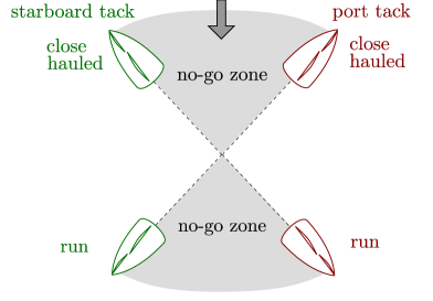
Figure 1: Points of sail.

For a given wind speed, the velocity of the yacht is a function of the angle between the wind direction and the yacht’s heading. This function is illustrated by polar diagrams, see Figure 2.

When we want to get closer to a particular point, say a buoy, then unless this point lies in the no-go zone with respect to the yacht, we can simply head directly towards it and this determines the tack on which to sail.

However, if the position of the buoy with respect to the yacht is in the no go zone, then the yacht has to follow a zigzag trajectory (see Fig. 3). This is called beating upwind: the yacht alternates between routes on starboard and on port tack while trying to sail with the optimal upwind angle, which is the angle in the polar diagram that maximizes the projection of the velocity vector onto the vertical axis (In Fig. 2, this is $\alpha_{0}=45^{o}$). Likewise, it is not optimal to aim directly at a buoy which lies leeward. The yacht will reach it more quickly by following zigzags of a given angle. The straight lines that cross the target buoy and that are parallel to the directions of these zigzags are called respectively the starboard and the port laylines.

In our model (see Fig. 2), we consider that the yacht’s behavior is symmetric if it is beating upwind or running downwind. The optimal angle for an upwind route is fixed at $45^{o}$, while for a downwind route, it is $135^{o}$. Between these angles, the yacht sails at constant speed $v>0$ and thus, the polar is a quarter of circle instead of the usual heart shaped curve, see Figure 2.

Figure 2: Example of a polar diagram with an 20 knots wind speed (on the left-hand side) and our modeling (on the right-hand side) where the optimal angle for an upwind route is fixed at $45^{o}$ and for a downwind route, at $135^{o}$.

When the yacht is beating upwind or running downwind, it must sail at angle $\alpha_{0}$ on one tack, then tack (resp. jibe), continue at angle $\alpha_{0}$ on the other tack and repeat this again until the target is reached (see Figure 3). Many possible tacking strategies can be employed, and in a constant wind, this does not affect the total distance traveled. However, each tack (resp. jibe) impacts the time required. In the present work the exact definition of a strategy and of a best “on average” strategy is going to be given.

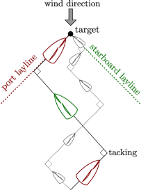
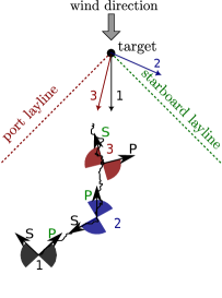
Figure 3: On the left hand side is an example of a tacking strategy for a boat beating upwind under a constant wind. A boat starting at the same point and following any other zigzag parallel to the laylines, would travel the same distance up to the target (dotted trajectory). On the right hand side is an example of a possible trajectory of the boat when the wind direction changes over time as indicated by the arrows at the top of the figure. The right-hand wings (resp. left-hand wings) of the butterfly shaped regions correspond to the feasible directions which can be achieved by sailing on port tack (resp. starboard tack).

In general, both the wind speed and the wind direction change over time. It turns out that moderate fluctuations of wind speed are less relevant than those of wind direction, so we assume that the wind speed is constant. For the wind direction, following [2], we assume that it follows a Brownian motion.

In order to describe the boat’s position, for mathematical simplicity, we have chosen to attach the reference frame to the wind instead of to geographic directions. In order to have an understanding of the problem in this new reference frame, assume first that the wind direction is constant and parallel to the vector $(1,1)\in\mathbb{R}^{2}$. The motion on starboard (resp. port) tack is shown on the right (resp. left) hand side of Figure 4, where the yacht is forced to tack (or jibe) on the half line $d^{+}$ (resp $d^{-}$) shown in the figure (since we will be interested in approaching the origin rather than moving away from it). The grey shaded areas represent the feasible headings of the boat. For each position of the boat and each tack, we choose the direction which points closest to the target. Therefore for each position of the boat, we will only allow two headings, one corresponding to port tack and the other corresponding to starboard tack.

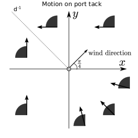
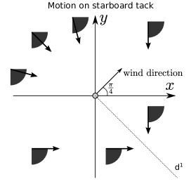
Figure 4: The sailboat’s motion on port tack on the left hand side and on starboard tack on the right hand side, from [14].

In a fluctuating wind, but with the reference frame attached to the wind, the wind is still represented by a constant vector that is parallel to the vector $(1,1)\in\mathbb{R}^{2}$, and it is the boat which is subject both to the displacement induced by sailing and to a Brownian rotation.In this description, a clockwise change of wind direction corresponds to a counterclockwise rotation of the boat’s position, and vice-versa.

2.2 Position Process

The purpose of this section is to write the position of the yacht as a 2-dimensional Itô process. In order to describe the motion in our model, we set

$$d^{1} =\{(x,y)\in\mathbb{R}^{2}:x=-y\mbox{ and }x>0\},$$ (2.1)

$$d^{-1} =\{(x,y)\in\mathbb{R}^{2}:x=-y\mbox{ and }x<0\},$$ (2.2)

and we split $\mathbb{R}^{2}_{*}=\mathbb{R}^{2}\setminus\{(0,0)\}$ into several zones (see Fig.5):

I $$=\{(x,y)\in\mathbb{R}^{2}_{*}:\,x\geq 0\mbox{ and }y\geq 0\},$$

II $$=\textsl{II}^{a}\cup\textsl{II}^{b}\cup d^{-1},$$

III $$=\{(x,y)\in\mathbb{R}^{2}_{*}:\,x\leq 0\mbox{ and }y\leq 0\},$$

IV $$=\textsl{IV}^{a}\cup\textsl{IV}^{b}\cup d^{1},$$

where

$$\textsl{II}^{a} =\{(x,y)\in\mathbb{R}^{2}:\,x<0\mbox{ and }y>-x\},$$

$$\textsl{II}^{b} =\{(x,y)\in\mathbb{R}^{2}:\,y>0\mbox{ and }y<-x\},$$

$$\textsl{IV}^{a} =\{(x,y)\in\mathbb{R}^{2}:\,y<0\mbox{ and }y>-x\},$$

$$\textsl{IV}^{b} =\{(x,y)\in\mathbb{R}^{2}:\,x>0\mbox{ and }y<-x\},$$

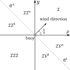
Figure 5: Race area and zones definition in the model of a Brownian wind.

Let $\sigma>0$ be a given number and $(B_{t})_{t\geq 0}$ be a standard real-valued Brownian motion defined on a filtered probability space $(\Omega,\mathcal{F},\{\mathcal{F}_{t}\}_{t\geq 0},\mathbb{P})$. In our model, $B_{t}$ represents the wind direction at time $t$.

Recall (see e.g. [7, p.65]) that if $\vec{\mu}_{c}$ and $\vec{\Sigma}$ are two functions from $\mathbb{R}^{2}$ in $\mathbb{R}^{2}$ defined by

$$\vec{\mu}_{c}(\vec{x})=-\tfrac{\sigma^{2}}{2}\,\,\vec{x}\qquad\text{ and }\qquad\vec{\Sigma}(\vec{x})=\vec{\Sigma}(x,y)=(-\sigma y,\sigma x),$$

then the unique solution $\vec{X}$ of the system of stochastic differential equations

$$d\vec{X}_{t}=\vec{\mu}_{c}(\vec{X}_{t})\,dt+\vec{\Sigma}(\vec{X}_{t})\,dB_{t},\qquad\vec{X}_{0}=\vec{x}=(x,y),$$

is a Brownian motion on the circle with speed $\sigma$, given by

$$\vec{X}_{t}=\left(\cos(\sigma B_{t})x-\sin(\sigma B_{t})y\,,\,\sin(\sigma B_{t})x+\cos(\sigma B_{t})y\right).$$

In the frame attached to the wind, the process $\vec{X}$ defines the position of a motionless yacht.

We now define the functions that correspond to each possible sailing direction of a moving yacht. For $\vec{x}\in\mathbb{R}^{2}$, set

$$\begin{array}[]{ccccc}&\vec{\mu}_{u}(\vec{x})=(0,v),&\text{(up)}&\qquad\vec{\mu}_{d}(\vec{x})=(0,-v),&\text{(down)}\\ &\vec{\mu}_{\ell}(\vec{x})=(-v,0),&\text{(left)}&\qquad\vec{\mu}_{r}(\vec{x})=(v,0),&\text{(right)}\\ &\vec{\mu}_{\rho}(\vec{x})=-v\frac{\vec{x}}{\|\vec{x}\|}.&\text{(radial)}\end{array}$$ (2.3)

The function corresponding to the starboard tack (resp. port tack) is denoted as $\vec{\mu}(\vec{x},1)$ (resp $\vec{\mu}(\vec{x},-1)$). According to Figures 4 and 5, we have

$$\vec{\mu}(\vec{x},1) =\vec{\mu}_{d}(\vec{x})\boldsymbol{1}_{\{\textsl{I}\cup\textsl{IV}^{a}\}}(\vec{x})+\vec{\mu}_{r}(\vec{x})\boldsymbol{1}_{\{\textsl{III}\cup\textsl{IV}^{b}\}}(\vec{x})+\vec{\mu}_{\rho}(\vec{x})\boldsymbol{1}_{\{\textsl{II}\}}(\vec{x})+\vec{\mu}_{c}(\vec{x}),$$ (2.4)

$$\vec{\mu}(\vec{x},-1) =\vec{\mu}_{\ell}(\vec{x})\boldsymbol{1}_{\{\textsl{I}\cup\textsl{II}^{a}\}}(\vec{x})+\vec{\mu}_{u}(\vec{x})\boldsymbol{1}_{\{\textsl{III}\cup\textsl{II}^{b}\}}(\vec{x})+\vec{\mu}_{\rho}(\vec{x})\boldsymbol{1}_{\{\textsl{IV}\}}(\vec{x})+\vec{\mu}_{c}(\vec{x}).$$ (2.5)

The position process of a yacht sailing on starboard tack, respectively on port tack, is now the solution of the following system of SDEs:

$$d\vec{X}_{t}=\vec{\mu}(\vec{X}_{t},1)\,dt+\vec{\Sigma}(\vec{X}_{t})\,dB_{t},\qquad\vec{X}_{0}=\vec{x}_{0},$$ (2.6)

respectively,

$$d\vec{X}_{t}=\vec{\mu}(\vec{X}_{t},-1)\,dt+\vec{\Sigma}(\vec{X}_{t})\,dB_{t},\qquad\vec{X}_{0}=\vec{x}_{0}.$$ (2.7)

The next two propositions lead to the solution of these SDEs.

Proposition 2.1.

Let $\vec{x}=(x,y)\in\mathbb{R}^{2}$ and $v_{1},v_{2}\in\mathbb{R}$. The process $(\vec{X}_{t}=(X_{t},Y_{t}))$, $t\in[0,+\infty[$, taking values in $\mathbb{R}^{2}$ and defined by

$$\vec{X}_{t}=\left(\begin{array}[]{c}\displaystyle\cos(\sigma B_{t})x-\sin(\sigma B_{t})y-v_{1}\int_{0}^{t}\cos(\sigma B_{t}-\sigma B_{s})ds+v_{2}\int_{0}^{t}\sin(\sigma B_{t}-\sigma B_{s})ds\\ \displaystyle\sin(\sigma B_{t})x+\cos(\sigma B_{t})y-v_{1}\int_{0}^{t}\sin(\sigma B_{t}-\sigma B_{s})ds-v_{2}\int_{0}^{t}\cos(\sigma B_{t}-\sigma B_{s})ds\end{array}\right)$$ (2.8)

is the unique solution of

$$\left\{\begin{array}[]{rll}dX_{t}&=\left(-\frac{\sigma^{2}}{2}\,X_{t}-v_{1}\right)\,dt-\sigma Y_{t}\,dB_{t},&\quad X_{0}=x,\\ dY_{t}&=\left(-\frac{\sigma^{2}}{2}\,Y_{t}-v_{2}\right)\,dt+\sigma X_{t}\,dB_{t},&\quad Y_{0}=y,\end{array}\right.$$ (2.9)

and its infinitesimal generator is given by

$${\cal L}_{\vec{X}}\phi=-\left(\tfrac{\sigma^{2}}{2}\,x+v_{1}\right)\frac{\partial\phi}{\partial x}-\left(\tfrac{\sigma^{2}}{2}\,y+v_{2}\right)\frac{\partial\phi}{\partial y}+\tfrac{\sigma^{2}}{2}\,y^{2}\,\frac{\partial^{2}\phi}{\partial x^{2}}-\sigma^{2}xy\frac{\partial^{2}\phi}{\partial x\partial y}+\tfrac{\sigma^{2}}{2}\,x^{2}\,\frac{\partial^{2}\phi}{\partial y^{2}}$$ (2.10)

where $\phi\in\mathcal{C}^{2}(\mathbb{R}^{2};\mathbb{R})$.

Proof.

Uniqueness follows directly from [7], Theorem 5.2.1 , since the drift, as well as the diffusion coefficient in (2.9), are affine. Moreover, [7, Thm. 7.3.3] yields (2.10). Thus, it only remains to verify that the process $\vec{X}$ defined by (2.8) is indeed a solution of (2.9) using Itô’s formula. For details see [14], Proposition 5.1.

∎

Proposition 2.2.

Let $\vec{x}=(x,y)\in\mathbb{R}^{2}_{*}$. The process $\left(\vec{X}_{t},\,t\in\left[0,\frac{\|\vec{x}\|}{v}\right]\right)$ taking values in $\mathbb{R}^{2}$ defined by

$$\vec{X}_{t}=\left(\begin{array}[]{c}X_{t}\\ Y_{t}\end{array}\right)=\left(\begin{array}[]{c}\left(\|\vec{x}\|-vt\right)\cos\left(\sigma B_{t}+\theta\right)\\ \left(\|\vec{x}\|-vt\right)\sin\left(\sigma B_{t}+\theta\right)\end{array}\right)$$ (2.11)

where $\theta\in\mathbb{R}$ is such that $\cos(\theta)=\frac{x}{\|\vec{x}\|}$ and $\sin(\theta)=\frac{y}{\|\vec{x}\|}$, is the unique solution of

$$\left\{\begin{array}[]{l l}dX_{t}&=\left(-\frac{\sigma^{2}}{2}\,X_{t}-\frac{vX_{t}}{\|\vec{X}_{t}\|}\right)\,dt-\sigma Y_{t}\,dB_{t},\qquad X_{0}=x,\\ dY_{t}&=\left(-\frac{\sigma^{2}}{2}\,Y_{t}-\frac{vY_{t}}{\|\vec{X}_{t}\|}\right)\,dt+\sigma X_{t}\,dB_{t},\qquad Y_{0}=y\end{array}\right.$$ (2.12)

and its infinitesimal generator is given by

$${\cal L}_{\vec{X}}\phi =-\left(\tfrac{\sigma^{2}}{2}\,x+\frac{vx}{\|\vec{x}\|}\right)\frac{\partial\phi}{\partial x}-\left(\tfrac{\sigma^{2}}{2}\,y+\frac{vy}{\|\vec{x}\|}\right)\frac{\partial\phi}{\partial y}+\tfrac{\sigma^{2}}{2}\,y^{2}\frac{\partial^{2}\phi}{\partial x^{2}}-\sigma^{2}xy\frac{\partial^{2}\phi}{\partial x\partial y}+\tfrac{\sigma^{2}}{2}\,x^{2}\frac{\partial^{2}\phi}{\partial y^{2}}$$ (2.13)

where $\phi\in\mathcal{C}^{2}(\mathbb{R}^{2};\mathbb{R})$.

Proof.

Observe that even if the drift coefficient in (2.12) is not Lipschitz continuous at $(0,0)$, the existence and the uniqueness of the solution holds on $[0,t_{0}]$, for all $0<t_{0}<\frac{\|\vec{x}\|}{v}$. As the process $\vec{X}$ defined by (2.11) hits $(0,0)$ at time $t=\frac{\|\vec{x}\|}{v}$, it is well-defined as a diffusion on the time interval $\left[0,\frac{\|\vec{x}\|}{v}\right]$. The formula (2.13) comes from (2.12) (see [7, Thm. 7.3.3]). It remains to verify that the process $\vec{X}$ defined by (2.11) is indeed a solution of (2.12). For details see [14], Proposition 5.2.

∎

We see that the system (2.12) can also be written

$$d\vec{X}_{t}=(\vec{\mu}_{c}(\vec{X}_{t})+\vec{\mu}_{\rho}(\vec{X}_{t}))\,dt+\sigma(\vec{X}_{t})\,dB_{t},\qquad\vec{X}_{0}=\vec{x},\quad t\in\left[0,\tfrac{\|\vec{x}\|}{v}\right],$$ (2.14)

which corresponds to the equation satisfied by the position process of a yacht sailing radially in direction of the buoy. This happens if the boat is sailing on port tack in the zone IV or on starboard tack in the zone II.

On the other hand, Proposition 2.1 gives us the system of SDEs and the corresponding solutions for the other four motions:

• downward motion ($v_{1}=0,v_{2}=v$) when the boat is on starboard tack in zone $\textsl{I}\cup\textsl{IV}^{a}$,

• upward motion ($v_{1}=0,v_{2}=-v$) when the boat is on port tack in zone $\textsl{II}^{b}\cup\textsl{III}$,

• leftward motion ($v_{1}=v,v_{2}=0$) when the boat is on port tack in zone $\textsl{I}\cup\textsl{II}^{a}$,

• rightward motion ($v_{1}=-v,v_{2}=0$) when the boat is on starboard tack in zone $\textsl{III}\cup\textsl{IV}^{b}$.

Therefore, Prop. 2.1 and Prop. 2.2 provide explicit formulas to describe the solution of (2.6) and (2.7).

Remark 2.3.

Denote $(X^{1}_{t},Y^{1}_{t})$ (resp. $(X^{-1}_{t},Y^{-1}_{t})$) the process defined by (2.6) (resp. (2.7)). Define $\tau^{a}_{f}:=\inf\{t:(X^{a}_{t},Y^{a}_{t})\in d^{a}\cup O\}$, $a\in\{-1,+1\}$ where $d^{1}$, and $d^{-1}$ are defined in (2.1). Let $\tau_{0}:=\inf\{t:(X^{a}_{t},Y^{a}_{t})\in O\}$ and $\tau^{a}_{f1}:=\inf\{t:(X^{a}_{t},Y^{a}_{t})\in d^{a}\}$, so $\tau^{a}_{f}=\tau_{0}\wedge\tau^{a}_{f1}$. We use the convention that $\inf\{\emptyset\}=+\infty$. Equation (2.6) (resp. (2.7)) have Lipschitz continuous coefficients in $\mathbb{R}^{2}\setminus d^{1}$ (resp. $\mathbb{R}^{2}\setminus d^{-1}$), therefore by a standard localization argument, there exists a strong solution until time $\tau^{1}_{f}$ (resp. $\tau^{-1}_{f}$), for any initial condition $\bar{x}_{0}=(x_{0},y_{0})\in\mathbb{R}^{2}\setminus d^{1}$ (resp $\bar{x}_{0}=(x_{0},y_{0})\in\mathbb{R}^{2}\setminus d^{-1}$). In particular, the solution $(X^{a}_{t},Y^{a}_{t})$ is well defined on the event $\{w\in\Omega:\,\tau_{0}(\omega)<+\infty,\,\tau^{a}_{f1}(\omega)=+\infty\}$, that is, when the solution hits the origin before the line $d^{a}$.

For later use, the equations of motion are also written in radial coordinates. For definiteness, we consider angles in $\left[-\frac{\pi}{4},\frac{7\pi}{4}\right[$ and the general case is then obtained by periodic extension. Let us consider, for instance, the process describing a yacht sailing downwind. Setting $v_{1}=0$ and $v_{2}=v$ in (2.8), we see that the position process $\vec{X}$ satisfies

$$\left\{\begin{array}[]{rll}dX_{t}&=-\frac{\sigma^{2}}{2}\,X_{t}\,dt-\sigma Y_{t}\,dB_{t},&\quad X_{0}=x,\\ dY_{t}&=\left(-\frac{\sigma^{2}}{2}\,Y_{t}-v\right)\,dt+\sigma X_{t}\,dB_{t},&\quad Y_{0}=y.\end{array}\right.$$ (2.15)

Applying Itô’s formula to $R_{t}=\sqrt{(X_{t})^{2}+(Y_{t})^{2}}$ and $\Theta_{t}=\arctan(Y_{t}/X_{t})$, we get, after simplification,

$$R_{t} =R_{0}-\int_{0}^{t}v\frac{Y_{s}}{R_{s}}\,ds=R_{0}-\int_{0}^{t}v\sin(\Theta_{s})\,ds$$

and

$$\Theta_{t} =\Theta_{0}-\int_{0}^{t}\frac{v\cos(\Theta_{s})}{R_{s}}\,ds+\int_{0}^{t}\sigma\,dB_{s}.$$

In other words, the process $(R_{t},\Theta_{t})$ satisfies

$$\left\{\begin{array}[]{rll}dR_{t}&=-v\sin(\Theta_{t})\,dt,&\hskip 21.52771ptR_{0}=\|\vec{x}\|,\\ d\Theta_{t}&=-\dfrac{v\cos(\Theta_{t})}{R_{t}}\,dt+\sigma\,dB_{t},&\hskip 21.52771pt\Theta_{0}=\arctan(y/x).\end{array}\right.$$

We do the same for all other sailing directions and we find that the position of the yacht in polar coordinates $(R^{a}_{t},\Theta^{a}_{t})_{t\geq 0}$, for $a\in\{-1,1\}$, is the solution of

$$\left\{\begin{aligned} dR^{a}_{t}&=\mu_{1}(\Theta^{a}_{t},a)\,dt,&\qquad\mbox{ on }\{t<\tau^{a}_{f}\},\\ d\Theta^{a}_{t}&=\mu_{2}(R^{a}_{t},\Theta^{a}_{t},a)\,dt+\sigma\,dB_{t},&\qquad\mbox{ on }\{t<\tau^{a}_{f}\},\end{aligned}\right.$$ (2.16)

where $\tau^{a}_{f},\tau^{a}_{f1}$ are defined in Remark 2.3, and $\vec{\mu}(r,\theta,a)=(\mu_{1}(\theta,a),\mu_{2}(r,\theta,a))$ is given for $\theta\in[-\tfrac{\pi}{4},\tfrac{7\pi}{4}[$ by

$$\vec{\mu}(r,\theta,1) =\vec{\mu}_{d}(r,\theta)\boldsymbol{1}_{\left\{\theta\in\left[-\tfrac{\pi}{4},\tfrac{\pi}{2}\right[\right\}}+\vec{\mu}_{\rho}(r,\theta)\boldsymbol{1}_{\left\{\theta\in\left[\tfrac{\pi}{2},\pi\right[\right\}}$$ (2.17)

$$\qquad+\vec{\mu}_{r}(r,\theta)\boldsymbol{1}_{\left\{\theta\in\left[\pi,\tfrac{7\pi}{4}\right[\right\}},$$ (2.18)

$$\vec{\mu}(r,\theta,-1) =\vec{\mu}_{\ell}(r,\theta)\boldsymbol{1}_{\left\{\theta\in\left[0,\tfrac{3\pi}{4}\right[\right\}}+\vec{\mu}_{u}(r,\theta)\boldsymbol{1}_{\left\{\theta\in\left[\tfrac{3\pi}{4},\tfrac{3\pi}{2}\right[\right\}}$$ (2.19)

$$\qquad+\vec{\mu}_{\rho}(r,\theta)\boldsymbol{1}_{\left\{\theta\in\left[-\tfrac{\pi}{4},0\right[\cup\left[\tfrac{3\pi}{2},\tfrac{7\pi}{4}\right[\right\}},$$ (2.20)

and extended to $\theta\in\mathbb{R}$ by $2\pi$-periodicity, with

$$\vec{\mu}_{d}(r,\theta) =\left(-v\sin\theta,-v\tfrac{\cos\theta}{r}\right), \qquad\vec{\mu}_{\ell}(r,\theta)=\left(-v\cos\theta,v\tfrac{\sin\theta}{r}\right),$$

$$\vec{\mu}_{u}(r,\theta)) =\left(v\sin\theta,v\tfrac{\cos\theta}{r}\right), \qquad\vec{\mu}_{r}(r,\theta)=\left(v\cos\theta,-v\tfrac{\sin\theta}{r}\right),$$

$$\vec{\mu}_{\rho}(r,\theta) =(-v,0).$$

Remark 2.4.

Even though the coefficients of (2.16) may explode near the origin, a solution up to time $\tau^{a}_{f}$ is well defined because of the corresponding result in Cartesian coordinates (see Remark 2.3). In particular, the solution $(R^{a}_{t},\Theta^{a}_{t})$ is well defined on the event $\{w\in\Omega:\,\tau_{0}(\omega)<+\infty,\,\tau^{a}_{f1}(\omega)=+\infty\}$, that is, when the solution hits the origin before the line $F_{1}^{a}$.

See Fig. 6 for the illustration of the sailing rules in polar coordinates.

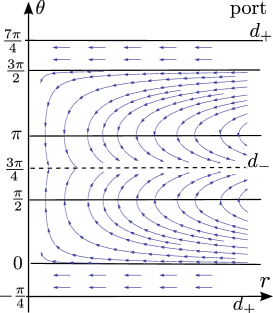
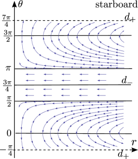
Figure 6: Sailing rules in polar coordinates. On the left-hand side, the yacht is on port tack ($a=-1$). On the right-hand side, the yacht is on starboard tack ($a=1$). The flow of arrows indicates the direction of the drift. In addition to the motion along the flow, the yacht moves as a Brownian motion in a direction parallel to the $\theta$-axis, with a speed that depends on the diffusion coefficient $\sigma$. Notice that there is no Brownian component in the radial direction.

3 Control Problem

In this section we will define a control problem that corresponds to minimizing the expected time to reach the circular target buoy $\mathbb{B}_{\eta}$ centered at the origin: $\mathbb{B}_{\eta}:=\{(x,y)\in\mathbb{R}^{2}:x^{2}+y^{2}\leq\eta^{2}\}$ (when $\eta=0$, then $\mathbb{B}_{\eta}$ reduces to a single point, the origin $O$). According to (2.16), set $\mu_{S,1}(\theta):=\mu_{1}(\theta,1)$ and $\mu_{S,2}(r,\theta):=\mu_{2}(r,\theta,1)$, so the motion of the boat on starboard tack, for $t\leq\tau^{1}_{f}$, is

$$\left\{\begin{array}[]{l l}dR_{t}=1_{\{R_{t}>0\}}\mu_{S,1}(\Theta_{t})dt,\\ d\Theta_{t}=1_{\{R_{t}>0\}}\mu_{S,2}(R_{t},\Theta_{t})dt+1_{\{R_{t}>0\}}\sigma dB_{t},\\ \end{array}\right.$$ (3.1)

where, according to (2.17)–(2.20), for $\theta\in[-\frac{\pi}{4},\frac{7\pi}{4}[$:

$$\mu_{S,1}(\theta)=\left\{\begin{array}[]{c}-v\sin(\theta),\\ -v,\\ v\cos(\theta),\end{array}\right.\qquad\mu_{S,2}(r,\theta)=\left\{\begin{array}[]{cl}-\frac{v\cos(\theta)}{r},&\qquad\theta\in[-\frac{\pi}{4},\frac{\pi}{2}[,\\ 0,&\qquad\theta\in[\frac{\pi}{2},\pi[,\\ -\frac{v\sin(\theta)}{r},&\qquad\theta\in[\pi,\frac{7\pi}{4}[,\end{array}\right.$$ (3.2)

and $\theta\rightarrow\mu_{S,1}(\theta),\theta\rightarrow\mu_{S,2}(r,\theta)$ are extended to $\mathbb{R}$ by $2\pi$-periodicity.

Similarly set $\mu_{P,1}(\theta):=\vec{\mu}_{1}(\theta,-1)$ and $\mu_{P,2}(r,\theta):=\vec{\mu}_{2}(r,\theta,-1)$, so the motion of the boat on port tack is, for $t\leq\tau^{-1}_{f}$,

$$\left\{\begin{array}[]{l l}dR_{t}=1_{\{R_{t}>0\}}\mu_{P,1}(\Theta_{t})dt,\\ d\Theta_{t}=1_{\{R_{t}>0\}}\mu_{P,2}(R_{t},\Theta_{t})dt+1_{\{R_{t}>0\}}\sigma dB_{t},\\ \end{array}\right.$$ (3.3)

where for $\theta\in[-\frac{\pi}{4},\frac{7\pi}{4}[,$:

$$\mu_{P,1}(\theta)=\left\{\begin{array}[]{c}-v,\\ -v\cos(\theta),\\ v\sin(\theta),\end{array}\right.\qquad\mu_{P,2}(r,\theta)=\left\{\begin{array}[]{cl}0,&\qquad\theta\in[\frac{3\pi}{2},\frac{7\pi}{4}[\cup[-\frac{\pi}{4},0[,\\ \frac{v\sin(\theta)}{r},&\qquad\theta\in[0,\frac{3\pi}{4}[,\\ \frac{v\cos(\theta)}{r},&\qquad\theta\in[\frac{3\pi}{4},\frac{3\pi}{2}[.\end{array}\right.$$

Therefore, according to (2.17)–(2.20),

$$\mu_{1}(\theta,a) =\mu_{S,1}(\theta)1_{\{a=1\}}+\mu_{P,1}(\theta)1_{\{a=-1\}},$$ (3.4)

$$\mu_{2}(r,\theta,a) =\mu_{S,2}(r,\theta)1_{\{a=1\}}+\mu_{P,2}(r,\theta)1_{\{a=-1\}}.$$ (3.5)

We recall that $c\geq 0$ denotes the tacking cost of the yacht. If $c=0$, there is no tacking cost, hence a strategy which allows an infinite number of tackings might still reach the island of radius $\eta$ in a finite amount of time. On the other hand, if $c>0$, then a reasonable strategy cannot have more that a finite number of tackings, otherwise the penalized time to the origin would be $\infty$. We distinguish three cases:

• $\eta>0$, $c=0$: here a strategy which allows an infinite number of tackings might reach the island of radius $\eta$ in a finite time. Since the current tack is irrelevant, the value function depends only on the position of the yacht in $\mathbb{R}^{2}$;

• $\eta=0$, $c=0$: here a strategy which allows an infinite number of tackings might reach the origin in a finite time. There is, however, an additional complication due to the fact that the coefficient $\mu_{2}(r,\theta,a)$ may converge to $\pm\infty$ as $r\rightarrow 0$ for some values of $a,\theta$. In this case also, the value function depends only on the position of the yacht in $\mathbb{R}^{2}$;

• $\eta\geq 0$, $c>0$: since the tacking cost is positive, a strategy under which the yacht reaches the origin in a finite amount of time a.s. cannot allow an infinite number of tackings. The space of admissible strategies will be slightly different and the value function depends on the position of the yacht and the current tack.

If $c=0$ and $\eta\geq 0$, the state equation and the space of admissible controls are defined in Definition 3.1. If $\eta=0$, we also need the notion of admissible strategy, introduced in Definition 3.6.

On the other hand, if $c>0$ and $\eta\geq 0$, an admissible strategy has to be piecewise constant, hence the existence of strong solution up to the origin is guaranteed, see Remarks 2.3 and 2.4, so we do not need to damp the coefficients of the state equation, see Definition 3.10.

3.1 Case $c=0$

Since the coefficients blow up near the origin (see (3.2) and (3.3)), even for $\eta>0$ it will be convenient to have the state equation defined on the whole $\mathbb{R}^{2}$. We therefore introduce the state equation below with damped coefficients. This approach also allows to consider the case $\eta=0$ as a limit case of the setting $\eta>0$.

Define

$$\phi_{n}(x):=\left\{\begin{array}[]{ll}0,&\qquad\text{if }x\leq\frac{1}{n+1},\\ n(n+1)x-n,&\qquad\text{if }x\in]\frac{1}{n+1},\frac{1}{n}[,\\ 1,&\qquad\text{if }x\geq\frac{1}{n},\end{array}\right.$$ (3.6)

and for $n\in\mathbb{N}$, consider the system of SDEs

$$\left\{\begin{array}[]{l l}dR^{n,A}_{t}=\phi_{n}(R^{n,A}_{t})\mu_{1}(\Theta^{n,A}_{t},A_{t})dt,\\ d\Theta^{n,A}_{t}=\phi_{n}(R^{n,A}_{t})\mu_{2}(R^{n,A}_{t},\Theta^{n,A}_{t},{A}_{t})dt+\phi_{n}(R^{n,A}_{t})\sigma dB_{t},\end{array}\right.$$ (3.7)

The position of the yacht at time $t$ driven by $A$, is defined as the $\mathbb{P}_{r,\theta,a}$ strong solution $(R_{t}^{A},\Theta_{t}^{A})_{t\in[0,+\infty[}$ of (3.7). where $\mathbb{P}_{r,\theta,a}$ denotes a family of probability measures such that

$$\mathbb{P}_{r,\theta,a}\left\{(R^{A}_{0},\Theta^{A}_{0})=(r,\theta),\,A_{0-}=a\right\}=1.$$ (3.8)

The initial tack $a$ is the yacht’s tack just before the race starts, so $A_{0}\neq A_{0-}$ if the yacht tacks immediately after the race starts.

Since $c=0$, the initial tack of the boat has no influence at all on the problem, hence we will omit it in (3.8), and write $\mathbb{P}_{r,\theta}$.

Definition 3.1.

Let $\eta\geq 0$, $(r,\theta)\in\mathbb{R}_{+}\times\mathbb{R}$ and $A:(\mathbb{R}_{+}\cup\{0-\})\times\Omega\mapsto\{+1,-1\}$ be a jointly measurable and adapted process in $(t,\omega)$. We say that $A$ is an admissible control if for every $n\in\mathbb{N}\setminus\{0\}$:

1. equation (3.7) admits a strong solution for $t\in[0,\infty[$,

2. $\mathbb{E}_{r,\theta}\left[\tau^{n,A}_{\eta}\right]<\infty$, where

   $$\tau^{n,A}_{\eta}:=\inf\left\{t:R^{n,A}_{t}\leq\tfrac{1}{n}\vee\eta\right\}.$$ (3.9)

The set of admissible controls under $\mathbb{P}_{r,\theta}$ is denoted by ${\cal A}^{\eta}_{r,\theta}$ (often the subscript $\cdot_{r,\theta}$ will be omitted).

In Section 4 we shall prove that, for every $\eta\geq 0$, the set ${\cal A}^{\eta}$ is non empty.

The above definition of an admissible control, while is also considering the case $\eta=0$, is not enough to tackle this setting because it does not ensure the existence of $\lim_{n\rightarrow\infty}(R^{n,A}_{\tau_{0}^{n,A}},\Theta^{n,A}_{\tau_{0}^{n,A}})$. For it to exist, we will need some additional conditions stated in Definition 3.6.

Remark 3.2.

We remark that, if $\eta=0$, then $\tau^{n,A}_{0}=\inf\left\{t:R^{n,A}_{t}\leq\tfrac{1}{n}\right\}$. In this case, we will write $\tau^{n,A}:=\tau^{n,A}_{0}$.

On the other hand, for $\eta>0$ and $n\geq n^{\eta}=:\inf\{n\in\mathbb{N}\setminus\{0\}:\eta\geq\frac{1}{n}\}$ , then $\tau^{n,A}_{\eta}=\inf\left\{t:R^{n,A}_{t}\leq\eta\right\}$, so it does not depend on $n$. For simplicity, we will write $\tau^{A}_{\eta}:=\tau^{n,A}_{\eta}$. Moreover note that, for $\eta>0$, we are only interested in the solution of (3.7) up to time $\tau^{A}_{\eta}$, and up to this time, for $n\geq n^{\eta}$, $\phi_{n}(R^{n,A}_{t})=1$.

The next Lemma proves that the solution to the damped equation (3.7) never attains the level $\frac{1}{n+1}$. This result will be used in the proof of Proposition 5.2.

Lemma 3.3.

Let $\eta\geq 0$, $(r,\theta)\in\mathbb{R}_{+}\times\mathbb{R}$ and $A\in{\cal A}^{\eta}_{r,\theta}$ be an admissible control. Without loss of generality, we assume that $v=1$ and $r\geq\frac{1}{n}\geq\frac{1}{n+1}\geq\eta$. Then for every $t\geq 0$,

$$\frac{1}{n+1}<R^{n,A}_{t},$$ (3.10)

where the inequality is strict.

Proof.

Let the stopping times be defined as

$$\rho^{n,A} :=\inf\{t:\,R^{n,A}_{t}\leq\frac{1}{n+1}\},$$ (3.11)

$$\sigma^{n,A,1} :=\inf\{t:\,R^{n,A}_{t}\leq\frac{1}{2}(\frac{1}{n}+\frac{1}{n+1})\},$$ (3.12)

$$\tilde{\sigma}^{n,A,1} :=\inf\{t\geq\sigma^{n,A,1}:\,R^{n,A}_{t}\geq\frac{1}{n}\}\wedge\rho^{n,A},$$ (3.13)

$$\sigma^{n,A,2} :=\inf\{t\geq\tilde{\sigma}^{n,A,1}:\,R^{n,A}_{t}\leq\frac{1}{2}(\frac{1}{n}+\frac{1}{n+1})\},$$ (3.14)

$$\tilde{\sigma}^{n,A,2} :=\inf\{t\geq\sigma^{n,A,2}:\,R^{n,A}_{t}\geq\frac{1}{n}\}\wedge\rho^{n,A},$$ (3.15)

$$\cdots$$ (3.16)

It will be proved that $\rho^{n,A}=+\infty$ a.s.

Assume that $\sigma^{n,A,i}(\omega)<\infty$. We wish to solve on the interval $t\in[\sigma^{n,A,i},\tilde{\sigma}^{n,A,i}]$ the integral equation

$$\tilde{R}^{n,i}_{t}=R^{n}_{\sigma^{n,A,i}}+\int_{0}^{t}[-n(n+1)\tilde{R}^{n,i}_{s}+n]ds,$$ (3.17)

which is equivalent to

$$\frac{d\tilde{R}^{n,i}_{t}}{dt}=[-n(n+1)\tilde{R}^{n,i}_{t}+n],\qquad\tilde{R}^{n,i}_{\sigma^{n,A,i}}=\frac{1}{2}(\frac{1}{n}+\frac{1}{n+1}).$$ (3.18)

This is a linear first order ODE whose solution is

$$\tilde{R}^{n,i}_{t} =e^{-n(n+1)t}\left(\int_{0}^{t}ne^{n(n+1)s}ds+C\right)$$ (3.19)

$$\qquad=e^{-n(n+1)t}\left(\frac{1}{n+1}(e^{n(n+1)t}-1)+C\right)$$ (3.20)

$$\qquad=\frac{1}{n+1}(1-e^{-n(n+1)t})+Ce^{-n(n+1)t}.$$ (3.21)

Imposing the initial condition $(\tilde{R}^{n,i}_{\sigma^{n,A,i}}=\frac{1}{2}(\frac{1}{n}+\frac{1}{n+1}))$ we get $C=\frac{1}{2}(\frac{1}{n}+\frac{1}{n+1})$, hence the solution can be rewritten as

$$\tilde{R}^{n,i}_{t} =\frac{1}{n+1}(1-e^{-n(n+1)t})+\frac{1}{2}(\frac{1}{n}+\frac{1}{n+1})e^{-n(n+1)t}$$ (3.22)

$$=\frac{1}{n+1}+\frac{1}{2}e^{-n(n+1)t}\left(\frac{1}{n}-\frac{1}{n+1}\right).$$ (3.23)

The second term is always positive and goes to zero as $t\rightarrow\infty$.

If $\sigma^{n,A,1}=\infty$ a.s, then also $\rho^{n,A}=+\infty$ a.s. Let $\omega$ be such that $\sigma^{n,A,1}(\omega)<\infty$, then on the interval $[\sigma^{n,A,1},\tilde{\sigma}^{n,A,1}]$ the process $R^{n}_{t}$ satisfies $R_{t}^{n}>\frac{1}{n+1}$, and

$$R^{n}_{t} =R^{n}_{\sigma^{n,A,1}}+\int_{0}^{t}[n(n+1)R^{n}_{s}-n]\mu_{1}(\Theta^{n}_{s},A_{s})ds$$ (3.24)

$$\geq R^{n}_{\sigma^{n,A,1}}+\int_{0}^{t}[-n(n+1)R^{n}_{s}+n]ds.$$ (3.25)

Since $\mu_{1}(r,a)\geq-1$ (here without loss of generality we assumed $v=1$), $R^{n}_{t}$ is greater than or equal to $\tilde{R}^{n,1}_{t}$ and in particular $R^{n}_{t}>\frac{1}{n+1}$, for $t\in[\sigma^{n,A,1},\tilde{\sigma}^{n,A,1}]$. If $\tilde{\sigma}^{n,A,1}=\infty$, then

$$R^{n}_{t}\geq\tilde{R}^{n,1}_{t}>\frac{1}{n+1},$$ (3.26)

and $\rho^{n,A}=\infty$. Otherwise if $\tilde{\sigma}^{n,A,1}<\infty$, for $t\in[\sigma^{n,A,1},\tilde{\sigma}^{n,A,1}]$:

$$R^{n}_{t}\geq\tilde{R}^{n,1}_{\tilde{\sigma}^{n,A,1}}>\frac{1}{n+1},$$ (3.27)

and $\rho^{n,A}>\tilde{\sigma}^{n,A,1}$. Let $\tilde{\sigma}^{n,A,1}<\infty$, it follows that $R^{n,1}_{\tilde{\sigma}^{n,A,1}}=\frac{1}{n}$. If $\sigma^{n,A,2}=\infty$, then

$$\rho^{n,A}\geq\sigma^{n,A,2}=\infty,$$ (3.28)

otherwise if $\sigma^{n,A,2}<\infty$, then on the interval $t\in[\sigma^{n,A,2},\tilde{\sigma}^{n,A,2}]$, we repeat the same argument as above. In particular, we observe that for all the $i$ for which $\tilde{\sigma}^{n,A,i}<\infty$, then $\rho^{n,A}>\tilde{\sigma}^{n,A,i}$.

Let $\bar{i}:=\inf\{i\in\mathbb{N}:\,\tilde{\sigma}^{n,A,i}=\infty\}$ with the convention that $\inf\{\emptyset\}=\infty$. There are two possible cases:

1. Case 1: $\bar{i}=\infty$, then $\rho^{n,A}>\tilde{\sigma}^{n,A,i}$ for every $i$. We observe that $\tilde{\sigma}^{n,A,i}-\sigma^{n,A,i}\geq\tau_{0}$, where $\tau_{0}$ is the time to exit $B(0,\frac{1}{n})$ starting from $\partial B(0,\frac{1}{2}(\frac{1}{n}+\frac{1}{n+1})))$ for the process $d\hat{R}_{t}=dt$, since $\mu_{1}<1$. It follows that $\tau_{0}\geq\frac{1}{2}(\frac{1}{n}+\frac{1}{n+1})$ and then $\tilde{\sigma}^{n,A,i}\geq\sum_{j=1}^{i}(\tilde{\sigma}^{n,A,j}-\sigma^{n,A,j})\geq i\tau_{0}$ for every $i$, so $\rho^{n,A}=\infty$.

2. Case 2: $\bar{i}<\infty$, then $\rho^{n,A}>\tilde{\sigma}^{n,A,\bar{i}-1}$ and $R^{n}_{t}\geq\tilde{R}^{n,\bar{i}-1}_{t}>\frac{1}{n+1}$ for every $t\geq\tilde{\sigma}^{n,A,\bar{i}-i}$, so $\rho^{n,A}=\infty$.

∎

3.1.1 Case $\eta>0$, $c=0$

We analyze first the case where $\eta>0$ and the tacking cost is null ($c=0$). This case is simpler than the case $\eta=0$, $c=0$, and $\eta\geq 0$, $c>0$ where many arguments used here do not apply directly.

If $A$ is an admissible control, we define the process

$$(R^{A}_{t},\Theta^{A}_{t}):=(R^{n^{\eta},A}_{t},\Theta^{n^{\eta},A}_{t}),\qquad t\in[0,\infty[,$$ (3.29)

where $n^{\eta}$ is defined in Remark 3.2.

The control problem ${\cal P}(\eta)$ consists in finding an admissible control that minimizes the expected time to reach the upwind buoy. Let, for $A\in{\cal A}^{\eta}$, and $\tau^{A}_{\eta}$ defined in Remark 3.2,

$$J^{\eta}(r,\theta,A)=\mathbb{E}_{r,\theta,a}\left[\tau^{A}_{\eta}\right]=\mathbb{E}_{r,\theta}\left[\tau^{A}_{\eta}\right],$$ (3.30)

where the last equality follows by the fact that tacking immediately after the race starts has no effect in the payoff function, then the value function is defined as

$$V^{\eta}(r,\theta)=\inf_{A^{\eta}\in{\cal A}^{\eta}}J^{\eta}(r,\theta,A).$$ (3.31)

In the above definition, $V^{\eta}:\mathbb{R}_{+}\times\mathbb{R}\to\mathbb{R}_{+}$ and $J^{\eta}:\mathbb{R}_{+}\times\mathbb{R}\times{\cal A}^{\eta}\to\mathbb{R}_{+}$, hence the control problem consists in finding an admissible control $A^{\star}$ which is optimal, that is $V^{\eta}(r,\theta)=J^{\eta}(r,\theta,A^{\star})$.

It remains to show that, for every $\eta>0$, the set ${\cal A}^{\eta}$ is non empty. Equivalently it remains to explicitly exhibit at least one process $A\in{\cal A}^{\eta}$ , $A:(\mathbb{R}_{+}\cup\{0-\})\times\Omega\mapsto\{+1,-1\}$ for which the system (3.7) admits a unique strong solution and $\tau^{A}_{\eta}<\infty$ a.s. This will be proved in Section 4.

The theorem below is the so called Verification Theorem. Having a candidate value function $\tilde{V}^{\eta}$, and a control $A^{\star}\in{\cal A}^{\eta}$ that is guessed to be optimal, it provides a sufficient condition for $\tilde{V}^{\eta}$ to be the value function of the problem ${\cal P}(\eta)$ and for the control $A^{\star}$ to be optimal. Let $N^{\eta}$ be defined in the following way:

$$N^{\eta}:\mathbb{R}_{+}\times\mathbb{R}_{+}\times\mathbb{R}\to\mathbb{R}_{+},\qquad N^{\eta}(t,r,\theta):=t+\tilde{V}^{\eta}(r,\theta),$$ (3.32)

for some function $\tilde{V}^{\eta}(r,\theta):\mathbb{R}_{+}\times\mathbb{R}\to\mathbb{R}_{+}$.

Theorem 3.4.

Fix $\eta>0$ and suppose there exists a continuous function $\tilde{V}^{\eta}(r,\theta):\mathbb{R}_{+}\times\mathbb{R}\to\mathbb{R}_{+}$ such that

1. $\tilde{V}^{\eta}(\eta,\theta)=0$ for all $\theta\in\mathbb{R}$,

2. $\tilde{V}^{\eta}$ is continuous at $r=\eta$, uniformly in $\theta\in\mathbb{R}$,

3. there exist $C,D\in\mathbb{R}_{+}$, such that for all $r\geq 0$, we have $\tilde{V}^{\eta}(r,\theta)\leq Cr+D$.

If

1. for all admissible controls $A\in{\cal A}^{\eta}$,

   $$N^{\eta}(t\wedge\tau^{A}_{\eta},R_{t\wedge\tau^{A}_{\eta}}^{A},\Theta_{t\wedge\tau^{A}_{\eta}}^{A})=t\wedge\tau^{A}_{\eta}+\tilde{V}^{\eta}(R_{t\wedge\tau^{A}_{\eta}}^{A},\Theta_{t\wedge\tau^{A}_{\eta}}^{A})$$ (3.33)

   is a submartingale, then $\tilde{V}^{\eta}(r,\theta)\leq V^{\eta}(r,\theta)$;

2. if, in addition, there is a control $A^{\star}\in{\cal A}^{\eta}$ for which

   $$N^{\eta}(t\wedge\tau^{A}_{\eta},R_{t\wedge\tau^{A^{\star}}_{\eta}}^{A^{\star}},\Theta_{t\wedge\tau^{A^{\star}}_{\eta}}^{A^{\star}})=t\wedge\tau^{A^{\star}}_{\eta}+\tilde{V}^{\eta}(R_{t\wedge\tau^{A^{\star}}_{\eta}}^{A^{\star}},\Theta_{t\wedge\tau^{A^{\star}}_{\eta}}^{A^{\star}})$$ (3.34)

   is a martingale, then $\tilde{V}^{\eta}(r,\theta)=V^{\eta}(r,\theta)$.

Proof.

Let $r$ and $\theta$ be fixed.

• We recall that an admissible control $A\in{\cal A}^{\eta}$ has the propety that $\mathbb{E}\left[\tau^{A}_{\eta}\right]<+\infty$.

  The submartingale property of $N^{\eta}(t\wedge\tau^{A}_{\eta},R^{A}_{t\wedge\tau^{A}_{\eta}},\Theta^{A}_{t\wedge\tau^{A}_{\eta}})$ implies, since $t\wedge\tau^{A}_{\eta}$ is a bounded stopping time,

  $$\tilde{V}^{\eta}(r,\theta) =\mathbb{E}\left[N^{\eta}(0,r,\theta)\right]\leq\mathbb{E}\left[N^{\eta}(t\wedge\tau^{A}_{\eta},R^{A}_{t\wedge\tau^{A}_{\eta}},\Theta^{A}_{t\wedge\tau^{A}_{\eta}})\right]$$ (3.35)

  $$=\mathbb{E}\left[(t\wedge\tau^{A}_{\eta})+\tilde{V}^{\eta}(R^{A}_{t\wedge\tau^{A}_{\eta}},\Theta^{A}_{t\wedge\tau^{A}_{\eta}})\right].$$ (3.36)

  Since, by definition of admissible control, $\tau^{A}_{\eta}<\infty$ $\mathbb{P}$-a.s., then $t\wedge\tau^{A}_{\eta}\rightarrow\tau^{A}_{\eta}$ a.s. as $t\rightarrow+\infty$. By the monotone convergence theorem, as $t\rightarrow\infty$,

  $$\mathbb{E}\left[t\wedge\tau^{A}_{\eta}\right]\rightarrow\mathbb{E}\left[\tau^{A}_{\eta}\right].$$ (3.37)

  Observe that $R^{A}_{t\wedge\tau^{A}_{\eta}}\rightarrow R^{A}_{\tau^{A}_{\eta}}=\eta$ as $t\rightarrow+\infty$. By the assumption of uniform continuity at $r=\eta$, and since $V^{\eta}(\eta,\cdot)=0$, then $V^{\eta}(R^{A}_{t\wedge\tau^{A}_{\eta}},\Theta^{A}_{t\wedge\tau^{A}_{\eta}})\rightarrow 0$ as $t\rightarrow+\infty$.

  By (3.4), we have that $\mu_{1}(\theta)\leq v$ for $\theta\in\mathbb{R}$. It follow that

  $$|R^{A}_{t\wedge\tau^{A}_{\eta}}-r|\leq v(t\wedge\tau^{A}_{\eta})\leq v\tau^{A}_{\eta},$$ (3.38)

  so

  $$R^{A}_{t\wedge\tau^{A}_{\eta}}\leq r+v\tau^{A}_{\eta}.$$ (3.39)

  By assumption (c):

  $$\tilde{V}^{\eta}(R^{A}_{t\wedge\tau^{A}_{\eta}},\Theta^{A}_{t\wedge\tau^{A}_{\eta}})\leq CR_{t\wedge\tau^{A}_{\eta}}+D\leq Cv\tau^{A}_{\eta}+Cr+D.$$ (3.40)

  Since $\mathbb{E}\left[\tau^{A}_{\eta}\right]<\infty$, we can apply the dominated convergence theorem to see that, as $t\rightarrow+\infty$,

  $$\mathbb{E}\left[\tilde{V}^{\eta}(R^{A}_{t\wedge\tau^{A}_{\eta}},\Theta^{A}_{t\wedge\tau^{A}_{\eta}})\right]\rightarrow 0.$$ (3.41)

  From (3.35), (3.37), (3.41), we conclude that

  $$\tilde{V}^{\eta}(r,\theta)\leq\mathbb{E}\left[\tau^{A}_{\eta}\right]=J^{\eta}(r,\theta,A).$$ (3.42)

  Since this holds for all $A\in{\cal A}^{\eta}$, by taking the infimum over $A$ it follows

  $$\tilde{V}^{\eta}(r,\theta)\leq V^{\eta}(r,\theta).$$ (3.43)

• Under the strategy $A^{\star}$

  $$\tilde{V}^{\eta}(r,\theta) =\mathbb{E}\left[N^{\eta}(0,r,\theta)\right]=\mathbb{E}\left[N^{\eta}(t\wedge\tau^{A^{\star}}_{\eta},R^{A^{\star}}_{t\wedge\tau^{A^{\star}}_{\eta}},\Theta^{A^{\star}}_{t\wedge\tau^{A^{\star}}_{\eta}})\right]$$ (3.44)

  $$=\mathbb{E}\left[t\wedge\tau^{A^{\star}}_{\eta}+\tilde{V}^{\eta}(R^{A^{\star}}_{t\wedge\tau^{A^{\star}}_{\eta}},\Theta^{A^{\star}}_{t\wedge\tau^{A^{\star}}_{\eta}})\right].$$ (3.45)

  Since by assumption $\mathbb{E}\left[\tau^{A^{\star}}_{\eta}\right]<\infty$ and $\tilde{V}^{\eta}(R^{A^{\star}}_{t},\Theta^{A^{\star}}_{t})\leq CR^{A^{\star}}_{t}+D\leq C(r+v\tau^{A^{\star}}_{\eta})+D$, the dominated convergence theorem applies as above so

  $$\lim_{t\rightarrow\infty}\mathbb{E}\left[t\wedge\tau^{A^{\star}}_{\eta}+\tilde{V}^{\eta}(R^{A^{\star}}_{t\wedge\tau^{A^{\star}}_{\eta}},\Theta^{A^{\star}}_{t\wedge\tau^{A^{\star}}_{\eta}})\right]$$ (3.46)

  $$=\mathbb{E}\left[\lim_{t\rightarrow\infty}(t\wedge\tau^{A^{\star}}_{\eta}+\tilde{V}^{\eta}(R^{A^{\star}}_{t\wedge\tau^{A^{\star}}_{\eta}},\Theta^{A^{\star}}_{t\wedge\tau^{A^{\star}}_{\eta}}))\right]=\mathbb{E}\left[\tau^{A^{\star}}_{\eta}\right],$$ (3.47)

  where the last equality follows as in Item (1) from hypotheses (a) and (b), hence

  $$\tilde{V}^{\eta}(r,\theta)=\mathbb{E}\left[\tau^{A^{\star}}_{\eta}\right].$$ (3.48)

  This implies

  $$\tilde{V}^{\eta}(r,\theta)=\mathbb{E}\left[\tau^{A^{\star}}_{\eta}\right]\geq\inf_{A\in{\cal A}^{\eta}}\mathbb{E}\left[\tau^{A}_{\eta}\right]=V^{\eta}(r,\theta),$$ (3.49)

  and by Item (1), it follows that

  $$\tilde{V}^{\eta}(r,\theta)=V^{\eta}(r,\theta).$$ (3.50)

∎

3.1.2 Case $\eta=0$, $c=0$

The case $\eta=0$, $c=0$ is more difficult because the drift of the process blows up at the origin, and, together with the fact that an admissible control might admit an infinite number of tackings on any compact set, it may lead to the failure of the usual integrability condition

$$\int_{0}^{\tau^{A}}|\mu_{2}(R^{A}_{t},\Theta^{A}_{t},A_{t})|dt,$$ (3.51)

but under appropriate control processes the following integral

$$\lim_{n\rightarrow\infty}\int_{0}^{\tau^{n,A}}\mu_{2}(R^{A}_{t},\Theta^{A}_{t},A_{t})dt$$ (3.52)

could exist and be finite. Through this subsection, let $A\in{\cal A}^{\eta}={\cal A}^{0}$.

Remark 3.5.

Since by definition of a control process, the solution of (3.7) is defined for every $t\in\mathbb{R}_{+}$, and in particular it is progressively measurable, then for any finite stopping time $\tau$ the process $(R^{n,A}_{t\wedge\tau},\Theta^{n,A}_{t\wedge\tau})$ is well defined. In particular, this means that

$$\left\{\begin{array}[]{l l}\int_{0}^{\tau}\phi_{n}(R^{n,A}_{t})\mu_{1}(\Theta^{n,A}_{t},A_{t})dt=R^{n,A}_{\tau},\\ \int_{0}^{\tau}\phi_{n}(R^{n,A}_{t})\mu_{2}(R^{n,A}_{t},\Theta^{n,A}_{t},A_{t})dt+\int_{0}^{\tau}\phi_{n}(R^{n,A}_{t})\sigma dB_{t}=\Theta^{n,A}_{\tau}.\end{array}\right.$$ (3.53)

Given an admissible control process $A$, consider the stopping time $\tau^{n,A}$, defined in Remark 3.2. For every $m\geq n>0$ we have

$$(R^{n,A}_{t\wedge\tau^{n,A}},\Theta^{n,A}_{t\wedge\tau^{n,A}})=(R^{m,A}_{t\wedge\tau^{n,A}},\Theta^{m,A}_{t\wedge\tau^{n,A}}),\qquad\mathbb{P}_{r,\theta}-a.s.,$$ (3.54)

so, for every $n>0$, we can define the process

$$(R^{A}_{t\wedge\tau^{n,A}},\Theta^{A}_{t\wedge\tau^{n,A}}):=(R^{n,A}_{t\wedge\tau^{n,A}},\Theta^{n,A}_{t\wedge\tau^{n,A}}),$$ (3.55)

where $(R^{A}_{t},\Theta^{A}_{t})_{t\in[0,\tau^{n,A}]}$ is a solution to

$$\left\{\begin{array}[]{l l}dR^{A}_{t}=1_{\{R^{A}_{t}>0\}}\mu_{1}(\Theta^{A}_{t},A_{t})dt,\\ d\Theta^{A}_{t}=1_{\{R^{A}_{t}>0\}}\mu_{2}(R^{A}_{t},\Theta^{A}_{t},A_{t})dt+1_{\{R^{A}_{t}>0\}}\sigma dB_{t},\\ (R_{0}^{A},\Theta_{0}^{A})=(r,\theta).\end{array}\right.$$ (3.56)

Moreover, observe that $\tau^{n,A}$ is increasing, so there exists $\tau^{A}$ such that $\tau^{n,A}\rightarrow\tau^{A}$ a.s. (possibly $\tau^{A}=\infty$). We can then define the stopping time

$$\tau^{A}:=\lim_{n\rightarrow\infty}\tau^{n,A}.$$ (3.57)

The below definition builds on top of Definition 3.1 and essentially requires that the controlled state equation is well behaved near the origin.

Definition 3.6.

Let $(r,\theta)\in\mathbb{R}_{+}\times\mathbb{R}$ and $A\in{\cal A}^{0}$ such that $\mathbb{E}_{r,\theta}\left[\tau^{A}\right]<\infty$ and the following limit exists

$$\lim_{n\rightarrow\infty}\left\{\begin{array}[]{l l}R^{A}_{\tau^{n,A}}\\ \Theta^{A}_{\tau^{n,A}}.\end{array}\right.$$ (3.58)

Then $A$ is said to be an admissible strategy. The limit will be denoted as $(R^{A}_{\tau^{A}},\Theta^{A}_{\tau^{A}})$ and in this case we say that the process $(R^{A}_{t},\Theta^{A}_{t})_{t\in[0,\tau^{A}[}$ is a solution to (3.7) in $[0,\tau^{A}[$. The set of admissible strategies under $\mathbb{P}_{r,\theta}$ is denoted by $\bar{{\cal A}}^{0}_{r,\theta}$ (often the subscript $\cdot_{r,\theta}$ will be omitted).

In Section 4 it is shown that the set of admissible strategies is non empty and the optimal control problem for $\eta=0$ has a finite value function.

Remark 3.7.

Let $A$ be an admissible strategy. Recalling once again that $R^{A}_{\tau^{n,A}}=\frac{1}{n}$, and

$$\lim_{n\rightarrow\infty}R^{A}_{t\wedge\tau^{n,A}}=R^{A}_{t\wedge\tau^{A}},$$ (3.59)

we must have $R^{A}_{\tau^{A}}=0$. Moreover, we can characterize $\tau^{A}$ as the first time $R^{A}_{t}$ hits the origin. Indeed, let $t<\tau^{A}$, then there exists $n$ such that $t\leq\tau^{n,A}$ so $R^{A}_{t}\geq\frac{1}{n}$ . This implies $R^{A}_{t}>0$ for all $t<\tau^{A}$. So we can define $\tau^{A}$ as:

$$\tau^{A}=\inf\{t:R^{A}_{t}=0\}.$$ (3.60)

Remark 3.8.

Since the limit $(R^{A}_{\tau^{A}},\Theta^{A}_{\tau^{A}})$ exists, then we can extend the process $(R^{A}_{t},\Theta^{A}_{t})$ on $\mathbb{R}_{+}$ in the following way

$$(R^{A}_{t},\Theta^{A}_{t}):=\left\{\begin{array}[]{l l}(R_{t}^{A},\Theta^{A}_{t})&\qquad t\in[0,\tau^{A}[,\\ (0,\Theta^{A}_{\tau^{A}})&\qquad t\geq\tau^{A}.\end{array}\right.$$ (3.61)

The control problem ${\cal P}(0)$ consists in finding an admissible strategy that minimizes the time to reach the upwind buoy. Letting

$$J^{0}(r,\theta,A)=\mathbb{E}_{r,\theta}\left[\tau^{A}\right]$$ (3.62)

then the value function is defined as

$$V^{0}(r,\theta)=\inf_{A\in\bar{{\cal A}}^{0}}J^{0}(r,\theta,A).$$ (3.63)

In the above definition, $V^{0}:\mathbb{R}_{+}\times\mathbb{R}\to\mathbb{R}_{+}$ and $J^{0}:\mathbb{R}_{+}\times\mathbb{R}\times\bar{{\cal A}}^{0}\to\mathbb{R}_{+}$, hence the control problem ${\cal P}$ consists in finding an admissible strategy $A^{\star}\in\bar{{\cal A}}^{0}$ such that $V^{0}(r,\theta)=J^{0}(r,\theta,A^{\star})$. Also in this case the value assumed by any strategy $A$ at time $0-$ has no influence at all on the payoff function and the value function, so we drop the dependency and write $V^{0}(r,\theta)$ instead of $V^{0}(r,\theta,a)$, and $J^{0}(r,\theta,A)$ instead of $J^{0}(r,\theta,a,A)$. In Section 4 we show that $\bar{{\cal A}}^{0}$ is non empty, and that the value function is finite.

As for the case $\eta>0$, a Verification Theorem is needed to prove that a candidate value function $\tilde{V}$, and a strategy $A^{\star}\in\bar{{\cal A}}^{0}$ that is guessed to be optimal, are de facto the value function of the problem ${\cal P}$ and an optimal strategy. We do not write the statement and the proof as it is enough to replace $\eta$ with $0$ in Theorem 3.4.

3.2 Case $\eta\geq 0$, $c>0$

This is the case where the tacking cost is positive. Here a strategy cannot allow an infinite number of tackings, hence it should be piecewise constant. The definition of admissible strategy takes into account that $c>0$.

Definition 3.9.

Let $X_{t}:[0,\infty[\times\Omega\rightarrow\mathbb{R}^{n}$ be a measurable, adapted and right continuous process. If, for every $\omega\in\Omega$ and $T<+\infty$, there exists $\varepsilon$ such that for all $s\in[0,T]:X_{s}\neq X_{s-}$, then $X_{r+s}=X_{s}$ for $r\in[0,\varepsilon]$, we say that $X$ is a piecewise constant process.

The yatch spends $c$ units of time when tacking. The total amount of time spent in tackings needs to be integrable for a strategy to be admissible. The main difference between Definition 3.10 and the definition of admissible control (see Definition 3.1) and admissible strategy (see Definition 3.6) given in the case $c=0$ is the restriction to piecewise constant processes and the condition on integrability of the number of tackings, formulated in Item (c).

Definition 3.10.

Let $\eta\geq 0$, $c>0$, $(r,\theta)\in\mathbb{R}_{+}\times\mathbb{R}$ and $a\in\{-1,+1\}$. Let $A:(\mathbb{R}_{+}\cup\{0-\})\times\Omega\mapsto\{+1,-1\}$ be a piecewise constant process such that:

1. the equation (3.64) below admits a $\mathbb{P}_{r,\theta,a}$ strong solution in $[0,\infty[$:

   $$\left\{\begin{array}[]{l l}dR^{A}_{t}=1_{\{R^{A}_{t}>0\}}\mu_{1}(\Theta^{A}_{t},A_{t})dt,\\ d\Theta^{A}_{t}=1_{\{R^{A}_{t}>0\}}\mu_{2}(R^{A}_{t},\Theta^{A}_{t},{A}_{t})dt+\sigma dB_{t},\end{array}\right.$$ (3.64)

2. $\mathbb{E}_{r,\theta,a}\left[\tau^{A}_{\eta}\right]$ is finite, where $\tau^{A}_{\eta}:=\inf\{t:R^{A}_{t}\leq\eta\}$.

3. $\mathbb{E}_{r,\theta,a}\left[M_{\tau^{A}_{\eta}}(A)\right]<\infty$, where

   $$M_{t}(A)=\#\{s\in[0,t]:\ A_{s}\neq A_{s-}\}.$$ (3.65)

The process $A$ is called an admissible strategy. The set of the admissible strategies under $\mathbb{P}_{r,\theta,a}$ (defined in (3.8)) is denoted by $\bar{{\cal A}}^{c,\eta}_{r,\theta,a}$ (often the subscript $\cdot_{r,\theta,a}$ will be omitted).

Remark 3.11.

Observe that, if $c>0$ and $\eta=0$, we do not need to damp the coefficients of the state equation (3.64). Indeed, given a piecewise continuous process, a sufficient condition for the existence of a strong solution to (3.64) is that (see Remark 2.3), for a $\delta>0$, $A_{t}=-1$ for $(R_{t}^{A},\Theta_{t}^{A})\in]0,+\infty[\times[-\frac{\pi}{4}-\delta,-\frac{\pi}{4}+\delta]$ and $A_{t}=+1$ for $(R_{t}^{A},\Theta_{t}^{A})\in]0,+\infty[\times[\frac{3\pi}{4}-\delta,\frac{3\pi}{4}+\delta]$. On the other hand, if we try to prove directly the existence of a solution to (3.7), for $\eta=0,c=0$, $t\in[0,+\infty[$, we immediately encounter the problem of non integrability of the coefficients near the origin for a wide class of control processes $A\in{\cal A}^{0}$.

Since a solution to (3.64) exists for all times, $\tau^{A}_{\eta}$ (see Remark 3.2 for its definition) is well defined, even for $\eta=0$ as

$$\tau^{A}_{\eta}:=\inf\left\{t:R^{A}_{t}\leq\eta\right\}.$$ (3.66)

In particular, for $\eta=0$, we do not need as well the concept of limit as in Definition 3.6. This is due again to the piecewise continuity of an admissible strategy. Indeed, even for $\eta=0$, the limit $\lim_{t\rightarrow\tau^{A}_{0}}(R^{A}_{t},\Theta^{A}_{t})$ exists because of the existence of the limit as $t\rightarrow\tau^{a}_{f}$ of (2.16), $a\in\{+1,-1\}$ (see Remark 2.3 and 2.4).

Remark 3.12.

Observe that, for $\eta>0$, $\bar{\cal A}^{c,0}\subset\bar{\cal A}^{0}\subset{\cal A}^{\eta}$, where $\bar{\cal A}^{0}$ and ${\cal A}^{\eta}$ are defined, respectively, in Definition 3.6 and 3.1.

The control problem ${\cal P}(c,\eta)$ consists in finding an admissible strategy that minimizes the time to reach the upwind buoy. Letting

$$J^{c,\eta}(r,\theta,a,A)=\mathbb{E}_{r,\theta,a}\left[\tau^{A}+cM_{\tau^{A}_{\eta}}(A)\right]$$ (3.67)

then the value function is defined as

$$V^{c,\eta}(r,\theta,a)=\inf_{A\in\bar{{\cal A}}^{c,\eta}}J^{\eta}(r,\theta,a,A).$$ (3.68)

In the above definition, $V^{c,\eta}:\mathbb{R}_{+}\times\mathbb{R}\times\{-1,+1\}\to\mathbb{R}_{+}$ and $J^{c,\eta}:\mathbb{R}_{+}\times\mathbb{R}\times\{-1,+1\}\times\bar{{\cal A}}^{c,\eta}\to\mathbb{R}_{+}$, hence the control problem ${\cal P}(c,\eta)$ consists in finding an admissible strategy $A^{\star}\in\bar{{\cal A}}^{c,\eta}$ such that $V^{c,\eta}(r,\theta,a)=J^{c,\eta}(r,\theta,a,A^{\star})$. In Section 4 we show that $\bar{{\cal A}}^{c,\eta}$ is non empty, and that the value function is finite.

4 Finiteness of the Value function

In this section we explicitly exhibit a strategy $A$ that belongs to $\bar{{\cal A}}^{c,\eta}$, for every $\eta\geq 0$. In view of Remark 3.12, $A$ also belongs to ${\cal A}^{\eta}\cap\bar{{\cal A}}^{0}$. In particular, this proves that that the three value functions (3.31),(3.63), and (3.68) are finite. The difficulty is to prove that it is possible to reach the origin with a finite number of tackings. We will work in polar coordinates for simplicity reasons. Firstly, we define a particular tacking strategy and prove that the payoff (3.67) for this strategy is finite for any starting point and $\eta=0$. Theorem 4.16 will be then a direct consequence of this.

Let $\alpha\in\left]0,\frac{\pi}{8}\right]$ and $r_{0}>0$. We define

$$D^{1} =\left([0,r_{0}[\,\times\left(\left[-\tfrac{\pi}{4},-\alpha\right]\cup\left[\tfrac{3\pi}{2}+\alpha,\tfrac{7\pi}{4}\right[\,\right)\right) \cup \quad\left(\{r_{0}\}\times\left(\left[-\tfrac{\pi}{4},0\right]\cup\left[\tfrac{3\pi}{2},\tfrac{7\pi}{4}\right[\,\right)\right)$$ (4.1)

$$D^{-1} =\left([0,r_{0}[\,\times\left[\tfrac{\pi}{2}+\alpha,\pi-\alpha\right]\right) \cup \quad\left(\{r_{0}\}\times\left[\tfrac{\pi}{2},\pi\right]\right)$$ (4.2)

and $C^{1}$, resp. $C^{-1}$, their complement sets in $[0,r_{0}]\times\left[-\tfrac{\pi}{4},\tfrac{7\pi}{4}\right[\,$ (see Fig. 7). We denote by $\bar{C}^{a}$ the closure of $C^{a}$. The idea of the strategy $A$ defined below is that as soon as the yatch touches the set $D^{1}$ (resp. $D^{-1}$) and is on starboard (resp. port) tack then it should tack. This is consistent with the definition of the forbidden lines $d^{1}$ and $d^{-1}$, see (2.1).

Suppose the initial position of the boat is $(r,\theta)$, $\theta\in]-\frac{\pi}{4},\frac{7\pi}{4}[$, with initial tack $a\in\{-1,+1\}$. Let the strategy $A$ be defined as $A_{0-}=a$, and

$$\left\{\begin{array}[]{l l}A_{0}=-1&\qquad\text{if}\ (r,\theta)\in D^{1},\\ A_{0}=1&\qquad\text{if}\ (r,\theta)\in D^{-1},\\ A_{0}=a&\qquad\text{elsewhere}.\end{array}\right.$$ (4.3)

Define $(R^{(1)}_{t},\Theta^{(1)}_{t})$ by $(R^{(1)}_{0},\Theta^{(1)}_{0})=(r,\theta)$, and for $t\in[0,\nu_{1}[$,

$$\left\{\begin{array}[]{l l}dR^{(1)}_{t}&=\mu_{1}(\Theta^{(1)}_{t},A_{0})dt,\\ d\Theta^{(1)}_{t}&=\mu_{2}(R^{(1)}_{t},\Theta^{(1)}_{t},A_{0})dt+\sigma dB_{t},\end{array}\right.$$ (4.4)

where

$$\nu_{1}:=\inf\left\{t\geq 0:\,\Theta_{t}^{(1)}\in D^{A_{0}}\right\}\wedge\tau^{(1)},$$ (4.5)

and

$$\tau^{(1)}=\inf\left\{t\geq 0:\,R_{t}^{(1)}=0\right\}\text{ if }\{\cdots\}\neq\emptyset\text{ else }+\infty.$$ (4.6)

Then define $(R^{(2)}_{t},\Theta^{(2)}_{t})$ by $(R^{(2)}_{\nu_{1}},\Theta^{(2)}_{\nu_{1}})=(R^{(1)}_{\nu_{1}},\Theta^{(1)}_{\nu_{1}})$, and for $t\in[\nu_{1},\nu_{2}[$,

$$\left\{\begin{array}[]{r l}dR^{(2)}_{t}&=\mu_{1}(\Theta^{(2)}_{t},-A_{0})dt,\\ d\Theta^{(2)}_{t}&=\mu_{2}(R^{(2)}_{t},\Theta^{(2)}_{t},-A_{0})dt+\sigma dB_{t},\end{array}\right.$$ (4.7)

where

$$\nu_{2}:=\inf\left\{t\geq\nu_{1}:\,\Theta_{t}^{(2)}\in D^{-A_{0}}\right\}\wedge\tau^{(2)},$$ (4.8)

and

$$\tau^{(2)}=\inf\left\{t\geq\nu_{1}:\,R_{t}^{(2)}=0\right\}\wedge\tau^{(1)}\text{ if }\{\cdots\}\neq\emptyset\text{ else }+\infty.$$ (4.9)

We remark that, if $\nu_{1}=\tau^{(1)}$, then also $\nu_{2}=\tau^{(2)}=\tau^{(1)}$.

Assuming $(R^{(i)}_{t},\Theta^{(i)}_{t})$ and $\nu_{i}$ have been defined, let $(R^{(i+1)}_{\nu_{i}},\Theta^{(i+1)}_{\nu_{i}})=(R^{(i)}_{\nu_{i}},\Theta^{(i)}_{\nu_{i}})$, and for $t\in[\nu_{i},\nu_{i+1}[$:

$$\left\{\begin{array}[]{ll}dR^{(i+1)}_{t}&=\mu_{1}(\Theta^{(i+1)}_{t},(-1)^{i}A_{0})dt,\\ d\Theta^{(i+1)}_{t}&=\mu_{2}(R^{(i+1)}_{t},\Theta^{(i+1)}_{t},(-1)^{i}A_{0})dt+\sigma dB_{t},\end{array}\right.$$ (4.10)

$$\nu_{i+1}:=\inf\left\{t\geq\nu_{i}:\,\Theta_{t}^{(i+1)}\in D^{(-1)^{i}A_{0}}\right\}\wedge\tau^{(i+1)},$$ (4.11)

and

$$\tau^{(i+1)}=\inf\left\{t\geq\nu_{i}:\,R_{t}^{(i+1)}=0\right\}\wedge\tau^{(i)}\text{ if }\{\cdots\}\neq\emptyset\text{ else }+\infty.$$ (4.12)

Observe that a strong solution to $(R^{(i+1)}_{t},\Theta^{(i+1)}_{t})_{t\in[\nu_{i},\nu_{i+1}[}$ exists since the process never hits the lines $d^{1}$ (resp. $d^{-1}$) when $(-1)^{i}=1$ (resp. $(-1)^{i}=-1$), hence the coefficients $\mu_{1}$ and $\mu_{2}$ are Lipschitz.

Let $\nu_{0}=0$. The process $(A_{t})_{t\in[0,+\infty[}$ is defined by $(A_{t})=(-1)^{i}A_{0}$ on $[\nu_{i},\nu_{i+1}[$. Define the stopping time $\tilde{\tau}^{A}$ as

$$\tilde{\tau}^{A}=\inf\{\tau^{(i)},i\in\mathbb{N}\setminus\{0\}\}$$ (4.13)

and

$$\tilde{i}=\inf\{i>0:\nu_{i}=\tilde{\tau}^{A}\}\text{ if }\{\cdots\}\neq\emptyset\text{ else }+\infty.$$ (4.14)

The event $\{\tilde{\tau}^{A}<\infty\}$ means that the yatch reaches the origin in a finite amount of time. Observe that, on this event, for $i\geq\tilde{i}$, then $\tau^{(i)}=\nu_{\tilde{i}}=\tau^{(\tilde{i})}$, so after tacking at $\nu_{\tilde{i}-1}$, the yacth reaches the buoy.

The process $(R^{A}_{t},\Theta^{A}_{t})_{i\in[0,\infty[}$ is defined as

$$(R^{A}_{t},\Theta^{A}_{t})=\left\{\begin{array}[]{ll}(R^{(i)}_{t},\Theta^{(i)}_{t})\,\,\text{ for }\,i\leq\tilde{i},\ t\in[\nu_{i-1},\nu_{i}[\\ (0,\Theta^{(\tilde{i})}_{\tilde{\tau}^{A}})\,\,\text{ for }\,t\geq\nu_{\tilde{i}}=\tilde{\tau}^{A}.\end{array}\right.$$ (4.15)

Now that the process $(R^{A}_{t},\Theta^{A}_{t})_{i\in[0,\infty[}$ is defined, it is also possible to define $\tau^{A}$ using (3.66) and it is straightforward to verify that $\tau^{A}=\tilde{\tau}^{A}$ a.s.

In order to show that $A$ satisfies Item (a) of Definition 3.10 we need to prove that it is piecewise continuous and that (3.64) admits a strong solution for $t\in[0,\infty[$.

Lemma 4.1.

The process $(A_{t})$ defined above is piecewise constant. In particular there exists a strong solution to $(R^{A}_{t},\Theta^{A}_{t})_{t\in[0,+\infty[}$ defined in (3.64), and, for every $n>0$, to $(R^{n,A}_{t},\Theta^{n,A}_{t})_{t\in[0,+\infty[}$ defined in (3.7).

Proof.

We show that $A$ is piecewise constant. Fix $\omega\in\Omega$ and $T<\infty$. In order for the control $A_{t}$ to switch from $\pm 1$ to $\mp 1$, it is required at least an increment greater than $\alpha$ of the Brownian motion, indeed it has to cross the interval $[\frac{3\pi}{2},\frac{3\pi}{2}+\alpha]$ or $[-\alpha,0]$, where the drift of the radial component is zero. By absolute continuity of the path of Brownian motion in $[0,T]$, for every $t_{1}$, for every $\varepsilon$, there exists $\delta:\,\forall|t_{1}-t_{2}|\leq\delta$, $|B_{t_{1}}-B_{t_{2}}|\leq\varepsilon$. Let $\varepsilon=\alpha$. Then, for each $i\leq i^{T}:=\inf\{i:\ \nu_{i}\geq T\}$, the holding times $\nu_{i}-\nu_{i-1}$ of the control are larger than $\delta$ and this proves that $A$ is piecewise constant.

Since the control is piecewise constant and the process never hits the lines $d^{1}$ (resp. $d^{-1}$) when $A=1$ (resp. $A=-1$), there exists a strong solution to (3.64) defined by (4.15). Fix $n\in\mathbb{N}\setminus\{0\}$ and replace $\mu_{1}$ and $\mu_{2}$ by, respectively, $\phi_{n}\mu_{1}$ and $\phi_{n}\mu_{2}$ in (4.10), where $\phi_{n}$ is defined in (3.6). Then the same argument as above proves that there exists a strong solution to (3.7). In particular, Item (a) of both Definition 3.1 and Definition 3.10 are satisfied. ∎

Observe that the symmetry of the problem allows us to consider only one tack. Indeed, in Cartesian coordinates, it is clear that the payoff function (3.67) satisfies, for all $(x,y)\in\mathbb{R}^{2}$,

$$J^{c,0}((x,y),1)=J^{c,0}((y,x),-1).$$ (4.16)

Likewise, in polar coordinates, we have, for all $(r,\theta)\in\mathbb{R}_{+}\times\left[-\tfrac{\pi}{4},\tfrac{7\pi}{4}\right[$,

$$J^{c,0}((r,\theta),1)=J^{c,0}\left(\left(r,\tfrac{\pi}{2}-\theta\right),-1\right),$$ (4.17)

where $\tfrac{\pi}{2}-\theta$ is considered modulo $2\pi$ in $\left[-\tfrac{\pi}{4},\tfrac{7\pi}{4}\right[\,$. Therefore, instead of considering two maps, one for each tack, as in Fig.6, we can consider only one map corresponding to the starboard tack. When the strategy $A$ makes the yacht tack, then the process $(R^{A}_{t},\Theta^{A}_{t})$ makes a jump in the same map so that $\Theta^{A}_{t}\in[-\alpha,\frac{3\pi}{2}+\alpha]$ for $t\geq 0$. Namely, if $(R^{A}_{t-},\Theta^{A}_{t-})\in\partial C^{1}$, then (see Fig. 7) $(R^{A}_{t},\Theta^{A}_{t})=(R^{A}_{t},\tfrac{\pi}{2}-\Theta^{A}_{t-})$. From now on, we will consider that the yacht is always on starboard tack and as a result of which we shorten the notations. For instance, $\mathbb{P}_{r,\theta,1}$ becomes $\mathbb{P}_{r,\theta}$.

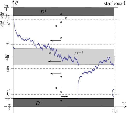
Figure 7: Tacking and continuation regions of the strategy $A$. The arrows indicate the direction and the intensity of the drift in the two directions $r$ and $\theta$. Each time the process hits $D^{1}$ (dark grey), $A$ tacks. We picture this by a jump to the symmetric point on $D^{-1}$ (light grey). Notice that $D^{1}$ contains the vertical segments $\{r_{0}\}\times\left[-\tfrac{\pi}{4},0\right]$ and $\{r_{0}\}\times\left[\tfrac{3\pi}{2},\tfrac{7\pi}{4}\right[\,$.

We recall that the drift functions for the starboard tack are defined in (3.2).

Remark 4.2.

If the initial radius satisfies $R^{A}_{0}\leq r_{0}$, we see that $R^{A}_{t}\leq r_{0}$ for all $t\geq 0$. (This will be proved rigorously later.) Moreover, notice that near the buoy ($r\approx 0$), the drift of the process $\Theta^{A}_{t}$ goes to $+\infty$, resp. $-\infty$ if $\Theta^{A}_{t}\in\left]\pi,\tfrac{3\pi}{2}+\alpha\right[$, resp. $\Theta^{A}_{t}\in\left]-\alpha,\tfrac{\pi}{2}\right[\,$, see (3.2). Therefore, the only way to reach the buoy is by arriving between $\tfrac{\pi}{2}$ and $\pi$ where there is no drift in the direction $\theta$.

Remark 4.3.

Notice the other symmetry condition given by

$$J^{c,0}((r,\theta),1)=J^{c,0}\left(\left(r,\tfrac{3\pi}{2}-\theta\right),1\right),\qquad\forall\,(r,\theta)\in\mathbb{R}_{+}\times\left[-\tfrac{\pi}{4},\tfrac{7\pi}{4}\right[\,,$$ (4.18)

where $\tfrac{3\pi}{2}-\theta$ is considered modulo $2\pi$ in $\left[-\tfrac{\pi}{4},\tfrac{7\pi}{4}\right[\,$.

Definition 4.4.

Let $(R^{A}_{t},\Theta^{A}_{t})$ denote the position of a yacht driven by $A$. We set $\sigma_{0}=\nu_{0}=\rho_{0}=\tau_{0}=0$, $E_{0}=\emptyset$ and for all $i\in\mathbb{N}^{*}$, we define

$$\begin{array}[]{ll}\tau^{A}&=\tau^{A}_{0}\\ \sigma_{i}&=\inf\left\{t\geq\tau_{i-1}:\Theta^{A}_{t}\notin\left[0,\,\tfrac{3\pi}{2}\right]\right\}\wedge\tau^{A}\\[4.30554pt] \nu_{i}&=\inf\left\{t\geq\tau_{i-1}:\Theta^{A}_{t}\notin\left[-\alpha,\,\tfrac{3\pi}{2}+\alpha\right]\right\}\wedge\tau^{A}\\[4.30554pt] \rho_{i}&=\inf\left\{t\geq\tau_{i-1}:R^{A}_{t}=r_{0}\right\}\wedge\tau^{A}\\ \tau_{i}&=\nu_{i}\wedge\rho_{i}\\ u_{i}&=\tau_{i}-\tau_{i-1}\\ \end{array}$$ (4.19)

and

$$E_{i}=\left\{\sup_{\tau_{i-1}\leq t\leq\tau^{A}}\left|\sigma B_{t}-\sigma B_{\tau_{i-1}}\right|<\tfrac{\alpha}{2}\right\}\subset\Omega.$$

The stopping times of (4.19) are illustrated in Fig.8. The times $\tau_{i}$ are the tacking times of the strategy $A$ and the event $E_{i}$ means that after the $(i-1)$-th tacking, the wind is calm (i.e. varies by no more than $\frac{\alpha}{2}$) until the end of the race.

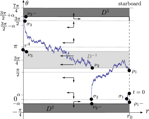
Figure 8: Stopping times of Definition 4.4. The position of the yacht at these different times is depicted with the bullet points.

Remark 4.5.

By definition, $\tau_{i}\leq\tau^{A}$ and if $\{\tau_{i}=\tau^{A}\}$ occurs, then $E_{i+1}$ occurs trivially.

Lemma 4.6.

There exists $K\in\mathbb{R}_{+}$ such that for all $i\in\mathbb{N}$ and for all $(r,\theta)\in\bar{C}^{1}$, the holding times $u_{i}$ of the strategy $A$ defined in (4.19) satisfy

$$\mathbb{E}_{r,\theta}\left(u_{i}\right)\leq K<+\infty.$$

Moreover, the stopping times $\sigma_{i},\,\nu_{i}$ and $\tau_{i}$ defined in (4.19) are integrable.

Proof.

Let $(r,\theta)\in\bar{C}^{1}$ be given numbers and let $f(x)=\left(x-\tfrac{3\pi}{4}\right)^{2}$. Then by Itô’s formula, we have

$$f\left(\Theta^{A}_{t\wedge\nu_{1}}\right)-f\left(\theta\right) =\int_{0}^{t\wedge\nu_{1}}\!\!2\mu_{2}\left(R^{A}_{s},\Theta^{A}_{s}\right)\left(\Theta^{A}_{s}-\tfrac{3\pi}{4}\right)ds$$ (4.20)

$$\qquad+2\sigma\int_{0}^{t\wedge\nu_{1}}\!\left(\Theta^{A}_{s}-\tfrac{3\pi}{4}\right)\,dB_{s}+\sigma^{2}(t\wedge\nu_{1}).$$ (4.21)

On one hand, $\Theta^{A}_{t}$ is bounded. On the other hand, for all $(r,\theta)\in\bar{C^{1}}$, $f\left(\theta\right)\leq\left(-\alpha-\tfrac{3\pi}{4}\right)^{2}$ and $\mu_{2}\left(r,\theta\right)\left(\theta-\tfrac{3\pi}{4}\right)\geq 0$ (see (3.2)). Hence, taking the expectation in the previous equation and using these inequalities, we find that $\sigma^{2}\mathbb{E}_{r,\theta}\left(t\wedge\nu_{1}\right)\leq 2\left(\alpha+\tfrac{3\pi}{4}\right)^{2}$. Therefore, by the monotone convergence theorem, we find that

$$\mathbb{E}_{r,\theta}\left(\nu_{1}\right)\leq 2\sigma^{-2}\left(\alpha+\tfrac{3\pi}{4}\right)^{2}=:K.$$

Observe that by definition of these stopping times, $\mathbb{E}_{r,\theta}(u_{1})=\mathbb{E}_{r,\theta}(\tau_{1})=\mathbb{E}_{r,\theta}(\rho_{1}\wedge\nu_{1})\leq\mathbb{E}_{r,\theta}(\nu_{1})$. Furthermore, by the strong Markov property, we have for all $i\in\mathbb{N}$,

$$\mathbb{E}_{r,\theta}(u_{i})=\mathbb{E}_{r,\theta}\left(\mathbb{E}_{r,\theta}\left(u_{i}\mid{\cal F}_{\tau_{i-1}}\right)\right)=\mathbb{E}_{r,\theta}\left(\mathbb{E}_{R^{A}_{\tau_{i-1}},\Theta^{A}_{\tau_{i-1}}}(u_{1})\right)\leq K.$$

Finally, $\nu_{i},\tau_{i},\sigma_{i}\leq\sum_{n=1}^{i}u_{i}$. Thus, all these stopping times are of finite expectation. ∎

Remark 4.7.

A consequence of this lemma is that without loss of generality, we can consider initial conditions $(r,\theta)$ such that $r\leq r_{0}$ and $\theta\in\,\left]\tfrac{\pi}{2}-\alpha,\tfrac{\pi}{2}+\alpha\right]$. Indeed, with at most one tacking and in a time with finite expectation, the yacht will be at

$$(R^{A}_{\tau_{1}},\Theta^{A}_{\tau_{1}})\in\left([0,r_{0}[\times\left\{\tfrac{\pi}{2}+\alpha,\pi-\alpha\right\}\right)\,\cup\,\left(\{r_{0}\}\times\left(\,\left]\tfrac{\pi}{2},\tfrac{\pi}{2}+\alpha\right]\cup[\pi-\alpha,\pi[\,\right)\right).$$

Moreover, by symmetry (see (4.18)), we can assume that

$$(R^{A}_{\tau_{1}},\Theta^{A}_{\tau_{1}})\in\left([0,r_{0}[\times\left\{\tfrac{\pi}{2}+\alpha\right\}\right)\,\cup\,\left(\{r_{0}\}\times\left]\tfrac{\pi}{2},\tfrac{\pi}{2}+\alpha\right]\right)$$

and this set is clearly included in $[0,r_{0}]\times\left]\tfrac{\pi}{2}-\alpha,\tfrac{\pi}{2}+\alpha\right]$.

Lemma 4.8.

If $\zeta$ denotes the following stopping time

$$\zeta=\inf\left\{t\geq 0:\Theta^{A}_{t}\notin\left[\tfrac{\pi}{2}-\alpha,\,\tfrac{\pi}{2}+\alpha\right]\right\}\wedge\tau^{A},$$ (4.22)

then, for all $(r,\theta)\in[0,r_{0}]\times\left]\tfrac{\pi}{2}-\alpha,\tfrac{\pi}{2}+\alpha\right]$,

$$R^{A}_{\zeta}\leq r\qquad\text{ and }\qquad\zeta\leq\frac{r}{v\cos\alpha},\qquad\mathbb{P}_{r,\theta}\text{-almost surely:}$$

Proof.

By (3.2), we have for all $0\leq t\leq\zeta$ that $\mu_{1}\left(\Theta^{A}_{t}\right)\in[-v,-v\cos\alpha]$. Hence,

$$0\leq R^{A}_{t\wedge\zeta}=r+v\int_{0}^{t\wedge\zeta}\mu_{1}\left(\Theta^{A}_{s}\right)\,ds\leq r-v\cos\alpha\,(t\wedge\zeta),\quad\forall\,t\geq 0.$$

Therefore, $R^{A}_{\zeta}\leq r$ and by dominated and monotone convergence, we have $\zeta\leq\frac{r}{v\cos\alpha}$. ∎

Lemma 4.9.

If the event $E_{1}$ occurs, then for all $(r,\theta)\in[0,r_{0}]\times\left]\tfrac{\pi}{2}-\alpha,\tfrac{\pi}{2}+\alpha\right]$, the following inequalities hold $\mathbb{P}_{r,\theta}$-almost surely.

$$\sigma_{1}-\zeta\leq\frac{d_{1}r}{v}\,,$$ (4.23a)

$$R^{A}_{\sigma_{1}}\leq c_{1}r,$$ (4.23b)

$$\tau_{1}-\sigma_{1}\leq\frac{d_{2}R^{A}_{\sigma_{1}}}{v}\,,$$ (4.23c)

$$R^{A}_{t}\leq c_{2}R^{A}_{\sigma_{1}},\qquad\quad\forall\,t\in[\sigma_{1},\tau_{1}],$$ (4.23d)

where

$$d_{1} =\sin\left(\tfrac{\alpha}{2}\right)\tan\alpha+1, c_{1}=\sqrt{1+\left(d_{1}-\cos\left(\tfrac{3\alpha}{2}\right)\right)^{2}-\cos^{2}\left(\tfrac{3\alpha}{2}\right)},$$

$$d_{2} =\frac{\left(\sin\left(\tfrac{\alpha}{2}\right)+\tan\alpha\right)\cos\alpha}{\cos(2\alpha)}, c_{2}=\sqrt{1+\left(d_{2}+\sin\left(\tfrac{\alpha}{2}\right)\right)^{2}-\sin^{2}\left(\tfrac{\alpha}{2}\right)}\,.$$

Proof.

In order to establish this statement, we will treat three cases separately.

Case 1: $R^{A}_{\zeta}=0$ (which is equivalent to $\zeta=\tau^{A}$). If $\zeta=\tau^{A}$, then $M_{\tau^{A}}(A)=0$, $\sigma_{1}=\nu_{1}=\rho_{1}=\tau_{1}=\tau^{A}$ and since $R^{A}_{\tau^{A}}=0$, the four inequalities are satisfied.

Case 2: $\Theta^{A}_{\zeta}=\tfrac{\pi}{2}+\alpha$ and $R^{A}_{\zeta}\neq 0$. Then, on the event $E_{1}$, we have, for all $t\geq\zeta$, that $\Theta^{A}_{t}\in\left[\tfrac{\pi}{2},\pi\right]$. Indeed, if we set

$$\eta=\left\{\begin{array}[]{ll}\inf\left\{t\geq\zeta:\Theta^{A}_{t}\notin\left[\tfrac{\pi}{2}\,,\pi\right]\right\},&\text{ if }\{\cdots\}\neq\emptyset,\\ +\infty,&\text{ otherwise},\\ \end{array}\right.$$

then, by (3.2) and (2.16), on $\{\eta<+\infty\}$,

$$\Theta^{A}_{\eta}=\Theta^{A}_{\zeta}+\int_{\zeta}^{\eta}\underbrace{\mu_{2}\left(R^{A}_{s},\Theta^{A}_{s}\right)}_{=0,\text{ since }s<\eta}\,ds+\underbrace{\sigma B_{\eta}}_{|\cdot|<\tfrac{\alpha}{2}}-\underbrace{\sigma B_{\zeta}}_{|\cdot|<\tfrac{\alpha}{2}}>\tfrac{\pi}{2}+\alpha-2\tfrac{\alpha}{2}=\tfrac{\pi}{2},$$

and similarly,

$$\Theta^{A}_{\eta}<\tfrac{\pi}{2}+\alpha+2\tfrac{\alpha}{2}=\tfrac{\pi}{2}+2\alpha<\pi.$$

Since $\Theta^{A}_{\eta}\in[\tfrac{\pi}{2},\pi]$ on $\{\eta<+\infty\}$, this shows that $\mathbb{P}\{\eta<+\infty\}=0$ and therefore, $\eta\equiv+\infty$. It follows that $\Theta^{A}_{t}\in\left[\tfrac{\pi}{2},\pi\right]$ for all $t\geq\zeta$. We have then by (3.2) that for all $t\geq\zeta$,

$$R^{A}_{t\wedge\tau^{A}}=R^{A}_{\zeta}+\int_{\zeta}^{t\wedge\tau^{A}}\underbrace{\mu_{1}\left(\Theta^{A}_{s}\right)}_{=-v}\,ds=R^{A}_{\zeta}-v(t\wedge\tau^{A}-\zeta).$$

Taking the limit when $t\rightarrow+\infty$, we find that $\tau^{A}-\zeta\leq\frac{R^{A}_{\zeta}}{v}\leq\frac{r}{v}$ by Lemma 4.8. Furthermore, since $\eta=+\infty$, we have $\sigma_{1}=\nu_{1}=\rho_{1}=\tau^{A}$, $M_{\tau^{A}}(A)=0$ and $R^{A}_{\sigma_{1}}=0$. Thus, the four inequalities (4.23a)-(4.23d) are also satisfied in this case.

Case 3: $\Theta^{A}_{\zeta}=\tfrac{\pi}{2}-\alpha$ and $R^{A}_{\zeta}\neq 0$. If $\Theta^{A}_{\zeta}=\tfrac{\pi}{2}-\alpha$ and $R^{A}_{\zeta}\neq 0$, then on $E_{1}$, we can show similarly as in the previous case that

$$\Theta^{A}_{t}\in\left[-\alpha,\tfrac{\pi}{2}\right[\,,\qquad\qquad\text{ for all }t\in[\zeta,\tau_{1}[\,.$$ (4.24)

Therefore, by Prop 2.1, in Cartesian coordinates the process $\vec{X}^{A}_{t}$ satisfies for all $t\in[\zeta,\tau_{1}[$

$$X^{A}_{t} =\cos(\sigma B_{t})X^{A}_{\zeta}-\sin(\sigma B_{t})Y^{A}_{\zeta}+v\int_{\zeta}^{t}\sin(\sigma B_{t}-\sigma B_{s})ds,$$

$$Y^{A}_{t} =\sin(\sigma B_{t})X^{A}_{\zeta}+\cos(\sigma B_{t})Y^{A}_{\zeta}-v\int_{\zeta}^{t}\cos(\sigma B_{t}-\sigma B_{s})ds.$$

On $E_{1}$, $|\sigma B_{t}|<\tfrac{\alpha}{2}$ for all $t\leq\tau^{A}$, thus, we can bound $X^{A}_{t}$ and $Y^{A}_{t}$ as follows

$$\cos\left(\tfrac{\alpha}{2}\right)X^{A}_{\zeta}-\sin\left(\tfrac{\alpha}{2}\right)Y^{A}_{\zeta}-v(t-\zeta)\sin\alpha<X^{A}_{t}<X^{A}_{\zeta}+\sin\left(\tfrac{\alpha}{2}\right)Y^{A}_{\zeta}+v(t-\zeta)\sin\alpha,$$

$$-\sin\left(\tfrac{\alpha}{2}\right)X^{A}_{\zeta}+\cos\left(\tfrac{\alpha}{2}\right)Y^{A}_{\zeta}-v(t-\zeta)<Y^{A}_{t}<\sin\left(\tfrac{\alpha}{2}\right)X^{A}_{\zeta}+Y^{A}_{\zeta}-v(t-\zeta)\cos\alpha,$$

for all $t\in[\zeta,\tau_{1}[\,$. Replacing $X^{A}_{\zeta}=R^{A}_{\zeta}\cos\left(\tfrac{\pi}{2}-\alpha\right)=R^{A}_{\zeta}\sin\alpha$ and $Y^{A}_{\zeta}=R^{A}_{\zeta}\cos\alpha$ in the second equation, we get

$$\cos\left(\tfrac{3\alpha}{2}\right)\,R^{A}_{\zeta}-v(t-\zeta)<Y^{A}_{t}<\left(\sin\left(\tfrac{\alpha}{2}\right)\sin\alpha+\cos\alpha\right)R^{A}_{\zeta}-v(t-\zeta)\cos\alpha.$$ (4.25)

Observe that, on $E_{1}$ and under our assumptions, $Y^{A}_{\sigma_{1}}=0$ and $\sigma_{1}<\tau_{1}$. Setting $t=\sigma_{1}$ in(4.25) and rearranging terms, we find

$$\cos\left(\tfrac{3\alpha}{2}\right)\,R^{A}_{\zeta}<v(\sigma_{1}-\zeta)<d_{1}\,R^{A}_{\zeta}.$$ (4.26)

We have thus by Lemma 4.8, $\sigma_{1}-\zeta<\tfrac{d_{1}r}{v}$ and this establishes inequality (4.23a) of the statement. Notice that if $\sigma_{1}=\tau^{A}$, then $\nu_{1}=\rho_{1}=\tau^{A}$, $R^{A}_{\sigma_{1}}=0$ and (4.23b)-(4.23d) are trivial, so from now on, we assume $\sigma_{1}<\tau^{A}$. By (4.24), on $E_{1}$, for all $t\in[\zeta,\tau_{1}[$, $R^{A}_{t}$ satisfies $dR^{A}_{t}=-v\sin\left(\Theta^{A}_{t}\right)\,dt=-v\frac{Y^{A}_{t}}{R^{A}_{t}}\,dt$. Hence, we have

$$d\left(R^{A}_{t}\right)^{2}=2R^{A}_{t}\,dR^{A}_{t}=-2vY^{A}_{t}\,dt,$$ (4.27)

and by (4.25),

$$\left(R^{A}_{t}\right)^{2} \leq\left(R^{A}_{\zeta}\right)^{2}-2v\int_{\zeta}^{t}\left(\cos\left(\tfrac{3\alpha}{2}\right)\,R^{A}_{\zeta}-v(s-\zeta)\right)\,ds$$

$$=\left(R^{A}_{\zeta}\right)^{2}+\left(v(t-\zeta)-\cos\left(\tfrac{3\alpha}{2}\right)\,R^{A}_{\zeta}\right)^{2}-\cos^{2}\left(\tfrac{3\alpha}{2}\right)\,\left(R^{A}_{\zeta}\right)^{2}.$$

Setting $t=\sigma_{1}$ and using (4.26), we get by Lemma 4.8 and by definition of $c_{1}$

$$\left(R^{A}_{\sigma_{1}}\right)^{2}\leq\left(R^{A}_{\zeta}\right)^{2}+\left(d_{1}R^{A}_{\zeta}-\cos\left(\tfrac{3\alpha}{2}\right)\,R^{A}_{\zeta}\right)^{2}-\cos^{2}\left(\tfrac{3\alpha}{2}\right)\,\left(R^{A}_{\zeta}\right)^{2}\leq r^{2}c_{1}^{2}$$

which establishes inequality (4.23b) of the statement.

On $E_{1}$, since $X^{A}_{\sigma_{1}}=R^{A}_{\sigma_{1}}$ and $Y^{A}_{\sigma_{1}}=0$, we have for all $t\in[\sigma_{1},\tau_{1}[$, by (2.8),

$$X^{A}_{t} =\cos(\sigma B_{t})R^{A}_{\sigma_{1}}+v\int_{\sigma_{1}}^{t}\sin(\sigma B_{t}-\sigma B_{s})ds,$$

$$Y^{A}_{t} =\sin(\sigma B_{t})R^{A}_{\sigma_{1}}-v\int_{\sigma_{1}}^{t}\cos(\sigma B_{t}-\sigma B_{s})ds,$$

and so $X^{A}_{t}\leq R^{A}_{\sigma_{1}}+v(t-\sigma_{1})\sin\alpha$ and

$$-\sin\left(\tfrac{\alpha}{2}\right)R^{A}_{\sigma_{1}}-v(t-\sigma_{1})\leq\;Y^{A}_{t}\;\leq\sin\left(\tfrac{\alpha}{2}\right)R^{A}_{\sigma_{1}}-v(t-\sigma_{1})\cos\alpha.$$ (4.28)

Since on this time interval, $X^{A}_{t}\tan\alpha+Y^{A}_{t}>0$, we find by combining these inequalities that

$$0<X^{A}_{t}\tan\alpha+Y^{A}_{t}\leq R^{A}_{\sigma_{1}}\left(\tan\alpha+\sin\left(\tfrac{\alpha}{2}\right)\right)+v(t-\sigma_{1})\left(\tan\alpha\sin\alpha-\cos\alpha\right),$$

which provides

$$t-\sigma_{1}\leq\frac{R^{A}_{\sigma_{1}}}{v}\,\frac{\tan\alpha+\sin\left(\tfrac{\alpha}{2}\right)}{\cos\alpha-\tan\alpha\sin\alpha}=\frac{R^{A}_{\sigma_{1}}}{v}\,d_{2}$$ (4.29)

by definition of $d_{2}$.Taking the limit $t\rightarrow\tau_{1}$, we obtain inequality (4.23c) of the statement.

Finally, by (4.27), we have that on $E_{1}$, for all $t\in[\sigma_{1},\tau_{1}[$

$$\left(R^{A}_{t}\right)^{2} =\left(R^{A}_{\sigma_{1}}\right)^{2}-2v\int_{\sigma_{1}}^{t}Y^{A}_{s}\,ds$$

(by (4.28)) $$\leq\left(R^{A}_{\sigma_{1}}\right)^{2}+2v\int_{\sigma_{1}}^{t}\left(\sin\left(\tfrac{\alpha}{2}\right)R^{A}_{\sigma_{1}}+v(s-\sigma_{1})\right)\,ds$$

$$=\left(R^{A}_{\sigma_{1}}\right)^{2}+\left(\sin\left(\tfrac{\alpha}{2}\right)\,R^{A}_{\sigma_{1}}+v(t-\sigma_{1})\right)^{2}-\sin^{2}\left(\tfrac{\alpha}{2}\right)\,\left(R^{A}_{\sigma_{1}}\right)^{2}$$

(by (4.29)) $$\leq\left(R^{A}_{\sigma_{1}}\right)^{2}\left(1+\left(\sin\left(\tfrac{\alpha}{2}\right)\,+d_{2}\right)^{2}-\sin^{2}\left(\tfrac{\alpha}{2}\right)\right)=\left(R^{A}_{\sigma_{1}}\right)^{2}c_{2}^{2}.$$

Since the process $R^{A}_{t}$ is continuous, this inequality remains true for $t=\tau_{1}$ and this establishes inequality(4.23d) of the statement. ∎

Lemma 4.10.

The constants $c_{1}$ and $c_{2}$ defined in Lemma 4.9 satisfy $c_{1}c_{2}<1$. Moreover, if the event $E_{1}$ occurs, then for all $(r,\theta)\in[0,r_{0}]\times\left]\tfrac{\pi}{2}-\alpha,\tfrac{\pi}{2}+\alpha\right]$, $R^{A}_{t}<r$ $\mathbb{P}_{r,\theta}$-almost surely for all $t\in[\sigma_{1},\tau_{1}]$.

Proof.

Long but direct computations show that

$$c_{1}^{2}c_{2}^{2}=\frac{1}{2} \left(1+\cos\alpha+2\left((1+\cos\alpha\sec(2\alpha))\sin\left(\tfrac{\alpha}{2}\right)+\sec(2\alpha)\sin(\alpha)\right)^{2}\right)$$

$$\times\left(1-\cos\left(\tfrac{3\alpha}{2}\right)^{2}+\left(1-\cos\left(\tfrac{3\alpha}{2}\right)+\sin\left(\tfrac{\alpha}{2}\right)\tan\alpha\right)^{2}\right).$$

where $\sec=\tfrac{1}{\cos}$. Furthermore, it can be shown that the term on the right-hand side is an increasing and positive function of $\alpha\in\left[0,\tfrac{\pi}{4}\right[$ approximately equal to $0.72$ at $\tfrac{\pi}{8}$. Since we assumed that $\alpha\leq\tfrac{\pi}{8}$, we conclude that $c_{1}c_{2}<1$. Finally, combining (4.23b) and (4.23d) of Lemma 4.9 with $c_{1}c_{2}<1$, we find directly that $R^{A}_{t}\leq c_{1}c_{2}r<r$ for all $t\in[\sigma_{1},\tau_{1}]$. ∎

Corollary 4.11.

For $i\in\mathbb{N}$, if $E_{i}$ occurs then, $\tau_{i}\leq\tau^{A}=\tau_{i+1}$ and $M_{\tau^{A}}(A)\leq i$ $\mathbb{P}_{r,\theta}$-a.s. for all $(r,\theta)\in[0,r_{0}]\times\left]\tfrac{\pi}{2}-\alpha,\tfrac{\pi}{2}+\alpha\right]$.

Proof.

If $\tau_{i}=\tau^{A}$ the proof is trivial, so we assume $\tau_{i}<\tau^{A}$. By Lemma 4.10 and by the strong Markov property, we have that $R^{A}_{t}<r_{0}$, $\mathbb{P}_{r,\theta}$-a.s. for all $t\in[\sigma_{i},\tau_{i}]$ on $E_{i}$. Thus, at time $\tau_{i}-$ the yacht hits the line $\theta=-\alpha$, $\nu_{i}<\rho_{i}$ and $\Theta^{A}_{\tau_{i}}=\tfrac{\pi}{2}+\alpha$. Again by the strong Markov property, this configuration is equivalent to the case 2 of the proof of Lemma 4.9. Therefore, on $E_{i}$, in this case we have that $\sigma_{i+1}=\nu_{i+1}=\tau_{i+1}=\tau^{A}$ and so $M_{\tau^{A}}(A)\leq i$. ∎

Corollary 4.12.

If $E_{1}$ occurs then, for all $(r,\theta)\in[0,r_{0}]\times\left]\tfrac{\pi}{2}-\alpha,\tfrac{\pi}{2}+\alpha\right]$,

$$\tau^{A}<(\sec\alpha+d_{1}+d_{2}+1)\,\frac{r_{0}}{v},\qquad\mathbb{P}_{r,\theta}\text{-almost surely.}$$

Proof.

Indeed, on $E_{1}$, we have by the preceding corollary that $M_{\tau^{A}}(A)\leq 1$, $\nu_{1}=\tau_{1}$ and $\Theta^{A}_{\tau_{1}}=\tfrac{\pi}{2}+\alpha$. Thus, by Lemma 4.8 and Lemma 4.9,

$$\tau^{A}=\zeta+(\sigma_{1}-\zeta)+(\tau_{1}-\sigma_{1})+(\tau^{A}-\tau_{1})\leq\frac{r_{0}}{v\cos\alpha}+\frac{d_{1}r_{0}}{v}+\frac{d_{2}r_{0}}{v}+(\tau^{A}-\tau_{1}),\;\mathbb{P}_{r,\theta}\text{-a.s.}.$$

Furthermore, on $E_{1}$, $\Theta^{A}_{t}\in\left[\tfrac{\pi}{2},\pi\right]$ for all $t\in[\tau_{1},\tau^{A}]$, hence $R^{A}_{t}=R^{A}_{\tau_{1}}-v(t-\tau_{1})$ and

$$\tau^{A}-\tau_{1}=\frac{R^{A}_{\tau_{1}}-R^{A}_{\tau^{A}}}{v}=\frac{R^{A}_{\tau_{1}}}{v}<\frac{r_{0}}{v}$$

which concludes the proof. ∎

Remark 4.13.

Lemmas 4.6, 4.8, 4.9, 4.10 and Corollary 4.11, 4.12 altogether tell us that, if from a tacking time $\tau_{i-1}$, the wind is calm for a sufficiently long time (that is $E_{i}$ occurs), then the yacht will reach the buoy with at most one tacking and in a bounded time. Moreover, if the wind is calm, then the yacht will never be pushed backwards into the circle $r=r_{0}$.

Proposition 4.14.

There exists $p_{0}\in\,]0,1[\,$, depending only on the parameters $\alpha,\sigma,v$ and $r_{0}$, such that for all $(r,\theta)\in[0,r_{0}]\times\left]\tfrac{\pi}{2}-\alpha,\tfrac{\pi}{2}+\alpha\right]$,

• $\mathbb{P}_{r,\theta}\left(\tau_{2}=\tau^{A}\right)\geq p_{0}$,

• $\mathbb{P}_{r,\theta}\left(\tau_{i}<\tau^{A}\right)\leq(1-p_{0})^{\frac{i}{2}}$ for all $i\in\mathbb{N},\,i\geq 2$.

Proof.

(a) Observe that by Corollary 4.11, $E_{1}\subset\left\{\tau_{2}=\tau^{A}\right\}$. Thus, by Corollary 4.12,

$$\mathbb{P}_{r,\theta}\left(\tau_{2}=\tau^{A}\right) \geq\mathbb{P}_{r,\theta}(E_{1})=\mathbb{P}_{r,\theta}\left(\sup_{0\leq t\leq\tau^{A}}\left|\sigma B_{t}\right|<\tfrac{\alpha}{2}\right)$$

$$\geq\mathbb{P}_{r,\theta}\left(\sup_{0\leq t\leq(\sec\alpha+d_{1}+d_{2}+1)\frac{r_{0}}{v}}\left|\sigma B_{t}\right|<\tfrac{\alpha}{2}\right)$$

$$=:p_{0}>0.$$

(b) Notice that $\left\{\tau_{i}<\tau^{A}\right\}\subset\left\{\tau_{i-1}<\tau^{A}\right\}\subset\cdots\subset\left\{\tau_{1}<\tau^{A}\right\}$, so by the strong Markov property and the previous point, we get

$$\mathbb{P}_{r,\theta}\left(\tau_{i}<\tau^{A}\right) =\mathbb{P}_{r,\theta}\left(\{\tau_{i}<\tau^{A}\}\cap\{\tau_{i-2}<\tau^{A}\}\right)$$

$$=\mathbb{E}_{r,\theta}\left(\boldsymbol{1}_{\{\tau_{i-2}<\tau^{A}\}}\,\mathbb{P}_{r,\theta}\left(\tau_{i}<\tau^{A}\mid{\cal F}_{\tau_{i-2}}\right)\right)$$

$$\leq\mathbb{P}_{r,\theta}(\tau_{i-2}<\tau^{A})(1-p_{0}).$$

The desired result is then obtained by induction. ∎

Proposition 4.15.

For all $(r,\theta)\in[0,r_{0}]\times\left]\tfrac{\pi}{2}-\alpha,\tfrac{\pi}{2}+\alpha\right]$,

• $\mathbb{E}_{r,\theta}\left(M_{\tau^{A}}(A)\right)<+\infty$,

• $\mathbb{E}_{r,\theta}\left(\tau^{A}\right)<+\infty$.

Proof.

(a) Notice that $\{M_{\tau^{A}}(A)>i\}\subset\{\tau_{i+1}<\tau^{A}\}$, thus, we have

$$\mathbb{E}_{r,\theta}\left(M_{\tau^{A}}(A)\right) =\sum_{i=0}^{\infty}\mathbb{P}_{r,\theta}\left(M_{\tau^{A}}(A)>i\right)\leq\sum_{i=0}^{\infty}\mathbb{P}_{r,\theta}\left(\tau_{i+1}<\tau^{A}\right)$$

$$\leq 1+\sum_{i=2}^{\infty}\mathbb{P}_{r,\theta}\left(\tau_{i}<\tau^{A}\right)\leq 1+\sum_{i=2}^{\infty}(1-p_{0})^{\frac{i}{2}}<+\infty$$

by Prop. 4.14.

(b) We have

$$\mathbb{E}_{r,\theta}\left(\tau^{A}\right) =\mathbb{E}_{r,\theta}\left(\sum_{i=0}^{M_{\tau^{A}}(A)}u_{i+1}\right)=\mathbb{E}_{r,\theta}\left(\sum_{k=0}^{\infty}\sum_{i=0}^{k}u_{i+1}\boldsymbol{1}_{\left\{M_{\tau^{A}}(A)=k\right\}}\right)$$

$$=\sum_{i=0}^{\infty}\mathbb{E}_{r,\theta}\left(\sum_{k=i}^{\infty}u_{i+1}\boldsymbol{1}_{\left\{M_{\tau^{A}}(A)=k\right\}}\right)=\sum_{i=0}^{\infty}\mathbb{E}_{r,\theta}\left(u_{i+1}\boldsymbol{1}_{\left\{M_{\tau^{A}}(A)\geq i\right\}}\right)$$

$$\leq\sum_{i=0}^{\infty}\mathbb{E}_{r,\theta}\left(\mathbb{E}_{r,\theta}\left(u_{i+1}\mid{\cal F}_{\tau_{i}}\right)\boldsymbol{1}_{\left\{\tau_{i}<\tau^{A}\right\}}\right).$$

Then, by the strong Markov property and by Lemma 4.6, we find that the right-hand side is smaller than

$$K\sum_{i=0}^{\infty}\mathbb{P}_{r,\theta}\left\{\tau_{i}<\tau^{A}\right\}\leq K\left(2+\sum_{i=2}^{\infty}(1-p_{0})^{\frac{i}{2}}\right)<+\infty$$

and the proof of Item (b) is complete.

∎

Theorem 4.16.

For every $\eta\geq 0$, $c\geq 0$ and every $(r,\theta,a)\in\mathbb{R}^{2}\times\{\pm 1\}$, $A\in{\cal A}^{\eta}\cap\bar{{\cal A}}^{0}\cap\bar{{\cal A}}^{c,\eta}$. In particular, the following are finite:

• $V^{c,\eta}(r,\theta,a)$, defined in (3.68),

• $V^{0}(r,\theta)$, defined in (3.63),

• $V^{\eta}(r,\theta,a),\ \eta>0$, defined in (3.31).

Proof.

We have shown that the strategy $A$ satisfies $\mathbb{E}_{r,\theta}\left(M_{\tau^{A}}(A)\right)<+\infty$ and $\mathbb{E}_{r,\theta}\left(\tau^{A}\right)<+\infty$ for all $(r,\theta)\in\mathbb{R}_{+}\times\left[-\tfrac{\pi}{4},\tfrac{7\pi}{4}\right[$. Indeed, even if Prop. 4.15 gives this property only for $(r,\theta)\in[0,r_{0}]\times\left]\tfrac{\pi}{2}-\alpha,\tfrac{\pi}{2}+\alpha\right]$, Remark 4.7 tells us that if the initial conditions are different, it is a matter of one tacking and of a finite expectation time to be in a favorable configuration. This, together with Lemma 4.1, shows that $A\in\bar{{\cal A}}^{c,\eta}$. Using Remark 3.12, it follow that $A\in{\cal A}^{\eta}\cup\bar{{\cal A}}^{0}$.

In particular, this proves that for every $\eta\geq 0$, $J^{c,\eta}(r,\theta,1,A)<+\infty$ (defined in (3.67)), which guarantees that $V^{c,\eta}(r,\theta,1)$ is finite for every $(r,\theta,a)$ as it is also bounded from below by 0. By symmetry, the same holds for $V^{c,\eta}(r,\theta,-1)$ so Item (a) is proved. Since $0\leq V^{\eta}(r,\theta)\leq V^{c,\eta}(r,\theta,a)$, Item (b) and Item (c) are also proved.

∎

5 Guess of the optimal strategy for $\eta\geq 0$ and $c=0$

In this section we guess an optimal strategy $A^{\star}$ in the case of null tacking cost and we prove that $A^{\star}$ is an admissible strategy in the sense of Definition 3.6. In order to do so, we first need to prove that the damped state equation (3.7) controlled by $A^{\star}$ has a unique strong solution. The coefficients are not Lipschitz, hence the standard result cannot be applied, but they exhibit a monotonicity property which allows us to prove strong uniqueness. We therefore apply the Yamada-Watanabe argument to show the existence of a strong solution to (3.7), for every $n\in\mathbb{N}^{\star}$. The existence of the limit in Definition 3.6 is non obvious and is proved in Lemma 5.3. In a companion paper it will be shown that the strategy is indeed optimal outside an island of radius $\eta>0$, depending on $v$ and $\sigma$. All the material of this section is taken from [1].

5.1 Guess of the strategy and symmetries of the problem

Let $\eta\geq 0$ and $(\theta,r)$ be the initial fixed starting point. The guess is that the optimal strategy has the following form.

Let $A^{\star}_{0-}(\theta)=a$ for a given $a\in\{-1,+1\}$, . We recall that, since we are in the setting $c=0$, that the initial tack has no influence. Then for $t\geq 0$, the feedback strategy $A_{t}^{\star}(\omega):=a^{\star}(\Theta_{t}(\omega))$, where $a^{\star}$ is defined as

$$a^{\star}(\theta)=\left\{\begin{array}[]{rll}1,&\theta\in[\frac{\pi}{4},\frac{5\pi}{4}[,\\ -1,&\theta\in[\frac{-3\pi}{4},\frac{\pi}{4}[,\end{array}\right.$$ (5.1)

and then extended on $\mathbb{R}$ by $2\pi$-periodicity. See also Figure 9 for a visual interpretation.

Under the strategy $A^{\star}$, the system (3.7) becomes

$$\left\{\begin{array}[]{l l}dR^{n,A^{\star}}_{t}=\phi_{n}(R_{t}^{n,A^{\star}})\mu^{\star}_{1}(\Theta^{n,A^{\star}}_{t})dt,\\ d\Theta^{n,A^{\star}}_{t}=\phi_{n}(R_{t}^{n,A^{\star}})\mu^{\star}_{2}(R^{n,A^{\star}}_{t},\Theta^{n,A^{\star}}_{t})dt+\phi_{n}(R_{t}^{n,A^{\star}})\sigma dB_{t},\\ (R_{0}^{n,A^{\star}},\Theta_{0}^{n,A^{\star}})=(r,\theta),\end{array}\right.$$ (5.2)

Hence, if $\theta\in[\frac{\pi}{4},\frac{5\pi}{4}[$, the yacht would sail on starboard tack, so

$$\mu^{\star}_{1}(\theta)=\mu_{1}(\theta,a^{\star}(\theta))=\left\{\begin{array}[]{cl}-v\sin(\theta)&\qquad\theta\in[\frac{\pi}{4},\frac{\pi}{2}[,\\ -v&\qquad\theta\in[\frac{\pi}{2},\pi[,\\ v\cos(\theta)&\qquad\theta\in[\pi,\frac{5\pi}{4}[,\\ \end{array}\right.$$ (5.3)

and

$$\mu^{\star}_{2}(r,\theta)=\mu_{2}(r,\theta,a^{\star}(\theta))=\left\{\begin{array}[]{cl}-\frac{v\cos(\theta)}{r}&\qquad\theta\in[\frac{\pi}{4},\frac{\pi}{2}[,\\ 0&\qquad\theta\in[\frac{\pi}{2},\pi[,\\ -\frac{v\sin(\theta)}{r}&\qquad\theta\in[\pi,\frac{5\pi}{4}[.\end{array}\right.$$ (5.4)

If $\theta\in[-\frac{3\pi}{4},\frac{\pi}{4}[$, the yatch would sail on port tack, therefore

$$\mu^{\star}_{1}(\theta)=\mu_{1}(\theta,a^{\star}(\theta))=\left\{\begin{array}[]{cl}v\sin(\theta)&\qquad\theta\in[-\frac{3\pi}{4},-\frac{\pi}{2}[,\\ -v&\qquad\theta\in[-\frac{\pi}{2},0[,\\ -v\cos(\theta)&\qquad\theta\in[0,\frac{\pi}{4}[,\\ \end{array}\right.$$ (5.5)

and

$$\mu^{\star}_{2}(r,\theta)=\mu_{2}(r,\theta,a^{\star}(\theta))=\left\{\begin{array}[]{cl}\frac{v\cos(\theta)}{r}&\qquad\theta\in[-\frac{3\pi}{4},-\frac{\pi}{2}[,\\ 0&\qquad\theta\in[-\frac{\pi}{2},0[,\\ \frac{v\sin(\theta)}{r}&\qquad\theta\in[0,\frac{\pi}{4}[.\end{array}\right.$$ (5.6)

Figure 9: On the left, guessed optimal strategy $A^{\star}$. The arrows indicate the direction of the optimal drift, and the dashed ones the direction of the drift under the strategy $-A^{\star}$. On the right, drift of the processes $R^{A^{\star}},\Theta^{A^{\star}}$ extended to $\mathbb{R}$ by $2\pi$-periodicity.

5.2 Existence of the process controlled by $A^{\star}$, case $\eta\geq 0$

Proving the existence and uniqueness of a solution of the system (5.2) controlled by the process $A^{\star}$ requires some care, because the function $\theta_{0}\rightarrow\mu_{2}(r,\theta)$ has discontinuities at

$$E:=\cup_{k\in\mathbb{Z}}E_{k},\qquad E_{k}:=\frac{\pi}{4}+k\pi,\ k\in\mathbb{Z},$$ (5.7)

therefore the standard results do not apply. In the present situation the coefficients satisfy a monotonicity property, see (5.13), but even the results which rely on this property assume continuity of the coefficients in the spatial coordinates, and hence are not applicable, see for example [6], Section 3. Our proof uses the classical Yamada-Watanabe procedure, therefore we first prove pathwise uniqueness, and then the existence of a weak solution.

The result is proved for $\eta\geq 0$. If $\eta>0$, part (a) is enough to show that $A$ is an admissible strategy, while if $\eta=0$ some more work is needed.

Lemma 5.1.

Let $u:\mathbb{R}\rightarrow\mathbb{R}$ be measurable and bounded, and fix $\delta>0$. If for every $|x_{1}-x_{2}|\leq\delta$, there exists a constant $C>0$ for which

$$(x_{1}-x_{2})(u(x_{1})-u(x_{2}))\leq C(x_{1}-x_{2})^{2},$$ (5.8)

then there exists $D>0$ such that for every $x_{1},x_{2}\in\mathbb{R}$,

$$(x_{1}-x_{2})(u(x_{1})-u(x_{2}))\leq D(x_{1}-x_{2})^{2}.$$ (5.9)

Proof.

Let $|x_{1}-x_{2}|\geq\delta$, and $M:=\sup_{x\in\mathbb{R}}|u(x)|$, then set $D:=\frac{2M}{\delta}\vee C$. This entails that

$$(x_{1}-x_{2})(u(x_{1})-u(x_{2}))\leq|x_{1}-x_{2}|2M\leq|x_{1}-x_{2}|\delta D\leq D(x_{1}-x_{2})^{2},$$ (5.10)

and if $|x_{1}-x_{2}|<\delta$, then trivially,

$$(x_{1}-x_{2})(u(x_{1})-u(x_{2}))\leq D(x_{1}-x_{2})^{2}.$$ (5.11)

∎

Before stating the main result of the section, we recall that the stopping times $\tau^{n,A}_{\eta}$ is defined in (3.9) and $\tau^{A}$ is defined in (3.57). We also recall that in this section we are assuming $c=0$. In a companion paper it will be proved the optimality of $A^{\star}$ for $\eta$ large enough.

Proposition 5.2.

Consider the system (5.2) for $\eta\geq 0$.

• Then for every $(r,\theta)\in\mathbb{R}_{+}\times\mathbb{R}$, $n\in\mathbb{N}^{\star}$, there exists a unique solution to (5.2) on $\mathbb{R}_{+}$. Moreover $\tau^{n,A^{\star}}_{\eta}\leq\sqrt{2}\frac{(r-\frac{1}{n})}{v}$ a.s. for every $n\in\mathbb{N}\setminus\{0\}$. In particular, if $\eta\geq 0$, then $A^{\star}$ is an admissible control, that is $A^{\star}\in{\cal A}^{\eta}$.

• Let $\eta=0$. Then $\tau^{A^{\star}}<\infty$ a.s and

  $$\lim_{n\rightarrow\infty}(R^{A^{\star}}_{\tau^{n,A^{\star}}},\Theta^{A^{\star}}_{\tau^{n,A^{\star}}})$$ (5.12)

  exists a.s. and the control process $A^{\star}$ is an admissible strategy, that is $A^{\star}\in\bar{{\cal A}}^{0}$.

Proof.

In the sequel, we will write $\mu_{1}(\theta)$ for $\mu_{1}(\theta)^{\star}$ and $\mu_{2}(r,\theta)$ for $\mu_{2}(r,\theta)^{\star}$. Below, the function $\phi_{n}(\theta)$ is the one defined in (3.6). It is necessary to show that $\mu_{1}$ and $\mu_{2}$ satisfy the monotonicity condition

$$\left(\begin{pmatrix}r_{1}\\ \theta_{1}\end{pmatrix}-\begin{pmatrix}r_{2}\\ \theta_{2}\end{pmatrix}\right)\cdot\left(\begin{pmatrix}\phi_{n}(r_{1})\mu_{1}(\theta_{1})\\ \phi_{n}(r_{1})\mu_{2}(r_{1},\theta_{1})\end{pmatrix}-\begin{pmatrix}\phi_{n}(r_{2})\mu_{1}(\theta_{2})\\ \phi_{n}(r_{2})\mu_{2}(r_{2},\theta_{2})\end{pmatrix}\right)$$ (5.13)

$$\qquad\leq K_{n}[(r_{1}-r_{2})^{2}+(\theta_{1}-\theta_{2})^{2}]$$ (5.14)

where $K_{n}$ is a constant depending on $n$. Since $(r,\theta)\rightarrow\phi_{n}(r)\mu_{1}(\theta)$ is Lipschitz on $\mathbb{R}^{2}$, and $r\rightarrow\phi_{n}(r)\mu_{2}(r,\theta)$ is Lipschitz (with Lipschitz constant that does not depend on $\theta$), it suffices to check that for fixed $r$, $(\theta_{1}-\theta_{2})(\mu_{2}(r,\theta_{1})-\mu_{2}(r,\theta_{2}))\leq(\theta_{1}-\theta_{2})^{2}$; in fact, (5.13) becomes (in the following the constant $C$ may vary from one occurrence to the other)

$$(r_{1}-r_{2})(\phi_{n}(r_{1})\mu_{1}(\theta_{1})-\phi_{n}(r_{2})\mu_{1}(\theta_{2}))$$ (5.15)

$$\qquad+(\theta_{1}-\theta_{2})(\phi_{n}(r_{1})\mu_{2}(r_{1},\theta_{1})-\phi_{n}(r_{2})\mu_{2}(r_{2},\theta_{2}))$$ (5.16)

$$=(r_{1}-r_{2})[\phi_{n}(r_{1})\mu_{1}(\theta_{1})-\phi_{n}(r_{2})\mu_{1}(\theta_{1})+\phi_{n}(r_{2})\mu_{1}(\theta_{1})-\phi_{n}(r_{2})\mu_{1}(\theta_{2})]$$ (5.17)

$$\qquad+(\theta_{1}-\theta_{2})[\phi_{n}(r_{1})\mu_{2}(r_{1},\theta_{1})-\phi_{n}(r_{2})\mu_{2}(r_{1},\theta_{1})$$ (5.18)

$$\qquad+\phi_{n}(r_{2})\mu_{2}(r_{1},\theta_{1})-\phi_{n}(r_{2})\mu_{2}(r_{2},\theta_{2})]$$ (5.19)

$$\leq(r_{1}-r_{2})\mu_{1}(\theta_{1})(\phi_{n}(r_{1})-\phi_{n}(r_{2}))+(r_{1}-r_{2})\phi_{n}(r_{2})(\mu_{1}(\theta_{1})-\mu_{1}(\theta_{2}))$$ (5.20)

$$\qquad+(\theta_{1}-\theta_{2})\mu_{2}(r_{1},\theta_{1})(\phi_{n}(r_{1})$$ (5.21)

$$\qquad-\phi_{n}(r_{2}))+(\theta_{1}-\theta_{2})\phi_{n}(r_{2})(\mu_{2}(r_{1},\theta_{1})-\mu_{2}(r_{2},\theta_{2}))$$ (5.22)

$$\leq C\mu_{1}(\theta_{1})(r_{1}-r_{2})^{2}+C|r_{1}-r_{2}||\theta_{1}-\theta_{2}|$$ (5.23)

$$\qquad+C|r_{1}-r_{2}||\theta_{1}-\theta_{2}|+\phi_{n}(r_{2})(\theta_{1}-\theta_{2})(\mu_{2}(r_{1},\theta_{1})-\mu_{2}(r_{2},\theta_{2})).$$ (5.24)

The last term is

$$\phi_{n}(r_{2})(\theta_{1}-\theta_{2})(\mu_{2}(r_{1},\theta_{1})-\mu_{2}(r_{2},\theta_{2}))$$ (5.25)

$$\qquad\leq\phi_{n}(r_{2})(\theta_{1}-\theta_{2})(\mu_{2}(r_{1},\theta_{1})-\mu_{2}(r_{2},\theta_{1})+\mu_{2}(r_{2},\theta_{1})-\mu_{2}(r_{2},\theta_{2}))$$ (5.26)

$$\qquad\leq C|\theta_{1}-\theta_{2}||r_{1}-r_{2}|+(\theta_{1}-\theta_{2})(\mu_{2}(r_{2},\theta_{1})-\mu_{2}(r_{2},\theta_{2})).$$ (5.27)

Recall the elementary inequality $ab\leq\frac{1}{2}(a^{2}+b^{2})$. Therefore in order to get the desired inequality (5.13), it is enough to prove that for fixed $r$, there exists a positive constant $C$ such that

$$(\theta_{1}-\theta_{2})(\mu_{2}(r,\theta_{1})-\mu_{2}(r,\theta_{2}))\leq C(\theta_{1}-\theta_{2})^{2}.$$ (5.28)

Let $F(\theta_{1},\theta_{2}):=(\theta_{1}-\theta_{2})(\mu_{2}(r,\theta_{1})-\mu_{2}(r,\theta_{2}))$. First observe that $F(\theta_{1},\theta_{2})=F(\theta_{2},\theta_{1})$, so it is enough to consider the case $\theta_{1}\leq\theta_{2}$. Moreover, by Lemma 5.1, it is enough to prove inequality (5.28) for $\theta_{1}$ close to $\theta_{2}$, say $|\theta_{1}-\theta_{2}|\leq\frac{\pi}{4}$. If $E_{k}\notin]\theta_{1},\theta_{2}[$, for any $k\in\mathbb{Z}$, then $\theta\rightarrow\mu_{2}(r,\theta)$ is Lipschitz and (5.28) follows. Now let $\theta_{1},\theta_{2}$ be such that for some $k\in\mathbb{Z}$, $E_{k}\in]\theta_{1},\theta_{2}[$. Since the function $\theta\rightarrow\mu_{2}(r,\theta)$ is periodic, it suffices to consider:

1. angles $\theta_{1},\theta_{2}$ such that $E_{1}=\frac{5\pi}{4}\in]\theta_{1},\theta_{2}[$, and $|\theta_{1}-\theta_{2}|\leq\frac{\pi}{4}$. This corresponds to $\theta_{1}\in\ ]\pi,\frac{5\pi}{4}[$ and $\theta_{2}\in]\frac{5\pi}{4},\frac{3\pi}{2}[$, and checking the definition of $\mu_{2}^{\star}$ for these values, the inequality to prove corresponds to

   $$v(\theta_{1}-\theta_{2})\left(-\frac{\sin\theta_{1}}{r}-\frac{\cos\theta_{2}}{r}\right)\leq 0,$$ (5.29)

   which holds since $\theta_{1}\leq\theta_{2}$;

2. angles $\theta_{1},\theta_{2}$ such that $E_{0}=\frac{\pi}{4}\in\ ]\theta_{1},\theta_{2}[$, and $|\theta_{1}-\theta_{2}|\leq\frac{\pi}{4}$. This corresponds to $\theta_{1}\in]0,\frac{\pi}{4}[$ and $\theta_{2}\in]\frac{\pi}{4},\frac{\pi}{2}[$, and checking the definition of $\mu_{2}^{\star}$ for these values, the inequality to prove corresponds to

   $$v(\theta_{1}-\theta_{2})\left(\frac{\sin\theta_{1}}{r}+\frac{\cos\theta_{2}}{r}\right)\leq 0,$$ (5.30)

   which holds since $\theta_{1}\leq\theta_{2}$.

The limiting cases $E_{k}\in\ ]\theta_{1},\theta_{2}]$, $E_{k}=\theta_{2}$ and $E_{k}\in[\theta_{1},\theta_{2}[$, $E_{k}=\theta_{1}$ have not been considered because the total amount of time spent by the process $\Theta^{A^{\star}}_{t}$ at $E_{k}$, $k\in\mathbb{Z}$, has zero Lebesgue measure.

1. In order to prove the existence and uniqueness of a strong solution, we first prove pathwise uniqueness and then the existence of a weak solution. Let $n$ be fixed and $\phi(s):=\phi_{n}(s),R_{t}:=R_{t}^{n,A^{\star}},\Theta_{t}:=\Theta_{t}^{n,A^{\star}}$. In all the above cases the monotonicity constant is bounded, say, by a positive constant that we call $C$. Let $(R_{t},\Theta_{t})$ and $(R^{\prime}_{t},\Theta^{\prime}_{t})$ be two solutions of the system (5.2). The optimal strategy $A^{\star}$ does not allow the monotonicity property (5.13) to hold if either $\Theta_{t}$ or $\Theta^{\prime}_{t}$ are on $E:=\cup_{k\in\mathbb{Z}}E_{k}$, but this is not relevant since the Lebesgue measure of the time spent by each of the processes on $E$ is zero. By Itô’s Lemma,

   $$\mathbb{E}\left[(R_{t}-R^{\prime}_{t})^{2}+(\Theta_{t}-\Theta^{\prime}_{t})^{2}\right]$$ (5.31)

   $$=2\mathbb{E}\left[\int_{0}^{t}[(R_{s}-R^{\prime}_{s})(\phi(R_{s})\mu_{1}(\Theta_{s})-\phi(R^{\prime}_{s})\mu_{1}(\Theta^{\prime}_{s}))\right.$$ (5.32)

   $$\qquad\left.+(\Theta_{s}-\Theta^{\prime}_{s})(\phi(R_{s})\mu_{2}(R_{s},\Theta_{s})-\phi(R^{\prime}_{s})\mu_{2}(R^{\prime}_{s},\Theta^{\prime}_{s}))]1_{\{\Theta_{s}\notin E,\,\Theta^{\prime}_{s}\notin E\}}ds\right]$$ (5.33)

   $$\qquad+2\mathbb{E}\left[\int_{0}^{t}(\Theta_{s}-\Theta^{\prime}_{s})(\phi(R_{s})-\phi(R^{\prime}_{s}))\sigma dW_{s}\right]$$ (5.34)

   $$\qquad+\mathbb{E}\left[\int_{0}^{t}(\phi(R_{s})-\phi(R^{\prime}_{s}))^{2}\sigma^{2}ds\right].$$ (5.35)

   Using the Lipschitz property of $\phi$ and the fact that the stochastic integral is a martingale, for some positive constants $C$ which might differ from one occurrence to the other,

   $$\mathbb{E}\left[(R_{t}-R^{\prime}_{t})^{2}+(\Theta_{t}-\Theta^{\prime}_{t})^{2}\right]$$ (5.36)

   $$\qquad\leq 2\int_{0}^{t}C\mathbb{E}\left[(R_{s}-R^{\prime}_{s})^{2}+(\Theta_{s}-\Theta^{\prime}_{s})^{2}\right]ds$$ (5.37)

   $$\qquad\qquad+C\mathbb{E}\left[\int_{0}^{t}(R_{s}-R^{\prime}_{s})^{2}\sigma^{2}ds\right]$$ (5.38)

   $$\qquad\leq\int_{0}^{t}C\mathbb{E}\left[(R_{s}-R^{\prime}_{s})^{2}+(\Theta_{s}-\Theta^{\prime}_{s})^{2}\right]ds.$$ (5.39)

   In order to prove the martingale property, since $R_{t}$ and $R^{\prime}_{t}$ are bounded, it suffices to show that

   $$\mathbb{E}\left[\int_{0}^{T}(\Theta_{t})^{2}dt\right]<\infty$$ (5.40)

   for every $T\in\mathbb{R}^{+}$.

   The drift of the process $(\Theta_{t})_{t\geq 0}$ is bounded for any $t$, in fact if $\eta=0$:

   $$\left|\phi(R_{t})\mu_{2}(R_{t},\Theta_{t})\right| \leq\frac{1}{R_{t}}(n(n+1)R_{t}-n)1_{\{R_{t}\leq\frac{1}{n}\}}+\frac{1}{R_{t}}1_{\{R_{t}>\frac{1}{n}\}}$$ (5.41)

   $$=(n(n+1)-\frac{n}{R_{t}})1_{\{R_{t}\leq\frac{1}{n}\}}+\frac{1}{R_{t}}1_{\{R_{t}>\frac{1}{n}\}}.$$ (5.42)

   Observe that for every $t\geq 0$, $R_{t}>\frac{1}{n+1}$ (see Lemma 3.3), therefore on the event $R_{t}\leq\frac{1}{n}$,

   $$0<(n(n+1)-\frac{n}{R_{t}})\leq n,$$ (5.43)

   which finally entails

   $$\left|\phi(R_{t})\mu_{2}(R_{t},\Theta_{t})\right|\leq n1_{\{\frac{1}{n+1}<R_{t}\leq\frac{1}{n}\}}+(n+1)1_{\{R_{t}>\frac{1}{n}\}}.$$ (5.44)

   Similar considerations are done for $\eta>0$.

   From (5.2) and (5.44), it follows that

   $$\mathbb{E}\left[\Theta_{t}\right]^{2} \leq 3\theta_{0}^{2}+3\mathbb{E}\left[\int_{0}^{t}\phi(R_{s})\mu_{2}(R_{s},\Theta_{s})ds\right]^{2}+3\mathbb{E}\left[\sigma\int_{0}^{t}\phi(R_{s})dW_{s}\right]^{2}$$ (5.45)

   $$\leq 3\theta_{0}^{2}+3t\mathbb{E}\left[\int_{0}^{t}(\phi(R_{s})\mu_{2}(R_{s},\Theta_{s}))^{2}ds\right]+3\sigma^{2}\mathbb{E}\left[\int_{0}^{t}(\phi(R_{s}))^{2}ds\right]<\infty,$$ (5.46)

   where we used the Cauchy-Schwartz inequality and the Itô’s isometry. Hence (5.40) is satisfied. From Equation (5.31), by the Grönwall’s inequality, a.s. for all $t\geq 0$,

   $$\mathbb{E}\left[(R_{t}-R^{\prime}_{t})^{2}+(\Theta_{t}-\Theta^{\prime}_{t})^{2}\right]\leq 0.$$ (5.47)

   This implies

   $$\mathbb{E}\left[(R_{t}-R^{\prime}_{t})^{2}+(\Theta_{t}-\Theta^{\prime}_{t})^{2}\right]=0$$ (5.48)

   therefore, since the process is continuous, pathwise uniqueness holds.

   We now prove the existence of a weak solution.

   Let $(B_{t})_{t\geq 0}$ be a standard Brownian motion on $(\Omega,{\cal F},({\cal F}_{t}),\mathbb{P})$, and

   $$\left\{\begin{array}[]{l l}dR_{t}=\phi(R_{t})\mu_{1}(\Theta_{t})dt,\\ d\Theta_{t}=\sigma dB_{t},\\ (R_{0},\Theta_{0})=(r,\theta).\end{array}\right.$$ (5.49)

   The coefficient $\phi(r)\mu_{2}(r,\theta)$ is bounded on $[\frac{1}{n+1},\infty[\times\mathbb{R}$ hence, for $t\in\mathbb{R}_{+}$, the process

   $$Z_{t}=\exp\left\{-\frac{1}{2}\int_{0}^{t}\frac{[\phi(R_{t})\mu_{2}(R_{s},\Theta_{s})]^{2}}{\sigma}ds+\int_{0}^{t}\frac{\phi(R_{t})\mu_{2}(R_{s},\Theta_{s})}{\sigma}dB_{s}\right\}$$ (5.50)

   is a martingale so that it is possible to define the probability $d\mathbb{Q}$ with Radon-Nykodyn derivative $\frac{d\mathbb{Q}}{d\mathbb{P}}|_{{\cal F}_{t}}=Z_{t}$ and by the Girsanov’s theorem

   $$dB^{\prime}_{t}=dB_{t}-\int_{0}^{t}\phi(R_{t})\mu_{2}(R_{s},\Theta_{s})ds$$ (5.51)

   is a Brownian motion on $[0,T]$, for every fixed $T<\infty$, on $(\Omega,{\cal F},({\cal F}_{t}),\mathbb{Q})$. Under this Brownian motion, equation (5.49) becomes

   $$\left\{\begin{array}[]{l l}dR_{t}=\phi(R_{t})\mu_{1}(\Theta_{t})dt,\\ d\Theta_{t}=\phi(R_{t})\mu_{2}(R_{t},\Theta_{t})+\sigma dB^{\prime}_{t},\\ (R_{0},\Theta_{0})=(r,\theta),\end{array}\right.$$ (5.52)

   so that $(R_{t},\Theta_{t})$ is a weak solution to (5.2) in $\mathbb{R}_{+}$.

   The last thing it remains to prove is that $\tau^{n,A^{\star}}_{\eta}<\infty$ for every $\eta\geq 0$ and $n\in\mathbb{N}\setminus\{0\}$. Without losing the generality we prove this fact for $\eta=0$, as the case $\eta>0$ easily follows.

   Case $\eta=0$. The process $R_{t}$ satisfies the equation

   $$R_{\tau^{n,A^{\star}}_{\eta}}=R_{0}+\int_{0}^{\tau^{n,A^{\star}}_{\eta}}\phi(R_{t})\mu_{1}(\Theta_{t})dt,$$ (5.53)

   hence $R$ does hit the ball of radius $\frac{1}{n}$ in a finite amount of time since it is easily seen that, if $R_{t}\geq\frac{1}{n}$, then $\phi(R_{t})=1$ and, by (5.3) and (5.5), it follows that $\mu_{1}(\theta)\leq-\frac{v}{\sqrt{2}}$ for every $\theta\in\mathbb{R}$, where $v$ is a constant. Therefore

   $$\frac{1}{n}=R_{\tau^{n,A^{\star}}_{\eta}}=R_{0}+\int_{0}^{\tau^{n,A^{\star}}_{\eta}}\mu_{1}(\Theta_{t})dt\leq R_{0}-\frac{v}{\sqrt{2}}\tau^{n,A^{\star}}_{\eta},$$ (5.54)

   so

   $$\tau^{n,A^{\star}}_{\eta}\leq\sqrt{2}\frac{(R_{0}-\frac{1}{n})}{v}.$$ (5.55)

2. By equation (5.55) it follows that $\tau^{A^{\star}}\leq\sqrt{2}\frac{R_{0}}{v}$. Let the process

   $$(R^{A^{\star}}_{t},\Theta^{A^{\star}}_{t}):=\lim_{n\rightarrow\infty}(R^{A^{\star}}_{t\wedge\tau^{n,A^{\star}}},\Theta^{A^{\star}}_{t\wedge\tau^{n,A^{\star}}}),$$ (5.56)

   for $t\in[0,\lim_{n\rightarrow\infty}\tau^{n,A^{\star}}[=[0,\tau^{A^{\star}}[$, where the right hand side is defined in (3.55). The proof that

   $$\lim_{t\rightarrow\tau^{A^{\star}}}(R^{A^{\star}}_{t},\Theta^{A^{\star}}_{t})$$ (5.57)

   exists a.s. is given in Lemma 5.3.

This concludes the proof. ∎

Lemma 5.3.

Let the process $(R^{A^{\star}}_{t},\Theta^{A^{\star}}_{t})$ as in (5.56), then

$$\lim_{t\rightarrow\tau^{A^{\star}}}(R^{A^{\star}}_{t},\Theta^{A^{\star}}_{t})$$ (5.58)

exists a.s.

Proof.

From now on $\tau:=\tau^{A^{\star}}$ and we will often omit the superscript $()^{A^{\star}}$. Since the process $R_{t}$ is bounded from below and decreasing, then it always has a limit, so in the rest of the proof it is shown that $\lim_{t\rightarrow\tau}\Theta_{t}$ exists and this proves that $A^{\star}$ is an admissible strategy. In particular, by Remark 3.7, it follows that $\lim_{t\rightarrow\tau}R_{t}=0$.

• $\forall k\in\mathbb{Z}$, $\forall\varepsilon>0$ the probability that $\Theta_{t}$ crosses $[\frac{k\pi}{2}-\varepsilon,\frac{k\pi}{2}+\varepsilon]$ infinitely many times is zero.

  Proof.

  Without loss of generality, suppose $k=0$. If $\Theta_{0}=\theta_{0}=-\varepsilon$, the equations of motion, for $t$ such that $\Theta_{t}\leq 0$, are

  $$\left\{\begin{array}[]{l l}dR_{t}=-vdt,\\ d\Theta_{t}=\sigma dB_{t},\\ (R_{0},\Theta_{0})=(r,-\varepsilon),\end{array}\right.$$ (5.59)

  and for $\Theta_{t}\geq 0$

  $$\left\{\begin{array}[]{l l}dR_{t}=-v\cos\Theta_{t}dt,\\ d\Theta_{t}=v\frac{\sin\Theta_{t}}{R_{t}}dt+\sigma dB_{t},\end{array}\right.$$ (5.60)

  so crossing from $-\varepsilon$ to $0$ requires a Brownian increment of $+\varepsilon$. For the same reason crossing from $\varepsilon$ to $-\varepsilon$ requires a Brownian increment greater than $-2\varepsilon$ since the drift is non negative. Since $\tau<+\infty$ a.s., and $t\rightarrow B_{t}$ is continuous, there can only be a finite number of such increments in $[0,\tau]$: indeed for all $\eta>0$, there is $\delta>0$ such that when $0<\tau-t<\delta$, then $|B_{t}-B_{\tau}|\leq\eta$, so all increments after time $\tau-\delta$ are smaller than $\eta$, then take $\eta<\varepsilon$. ∎

• $\liminf_{t\nearrow\tau}\Theta_{t}>-\infty,\qquad\limsup_{t\nearrow\tau}\Theta_{t}<+\infty.$

  Proof.

  Otherwise, $\Theta_{t}$ would cross infinitely many intervals $[\frac{k\pi}{2}-\varepsilon,\frac{k\pi}{2}+\varepsilon]$, and each requires a Brownian increment of size $\pm\varepsilon$. ∎

• For $\varepsilon>0$ let

  $$j_{\varepsilon}:=\sup\left\{j\in\mathbb{Z}:\,\liminf_{t\nearrow\tau}\Theta_{t}\geq\frac{j\pi}{2}-\varepsilon\right\}$$ (5.61)

  and

  $$k_{\varepsilon}:=\inf\left\{k\in\mathbb{Z}:\,\limsup_{t\nearrow\tau}\Theta_{t}\leq\frac{k\pi}{2}+\varepsilon\right\},$$ (5.62)

  then

  $$j_{\varepsilon}=k_{\varepsilon}\qquad\text{or}\qquad j_{\varepsilon}+1=k_{\varepsilon}.$$ (5.63)

  Proof.

  Otherwise $j_{\varepsilon}+2\leq k_{\varepsilon}$, so $\liminf_{t\nearrow\tau}\Theta_{t}\leq\frac{(j+1)\pi}{2}-\varepsilon$, $\limsup_{t\nearrow\tau}\Theta_{t}\geq\frac{(k-1)\pi}{2}+\varepsilon$, and $j+1\leq k-1$, so the interval $[\frac{(j+1)\pi}{2}-\varepsilon,\frac{(k-1)\pi}{2}+\varepsilon]$ would be crossed infinitely often. ∎

  By Item (3), $\lim\sup_{t\nearrow\tau}\Theta_{t}\leq\frac{(j_{\varepsilon}+1)\pi}{2}+\varepsilon$.

• Let

  $$F_{j,\varepsilon} :=\left\{\frac{j\pi}{2}-\varepsilon\leq\liminf_{t\nearrow\tau}\Theta_{t},\,\frac{j\pi}{2}+\varepsilon<\limsup_{t\nearrow\tau}\Theta_{t}\leq\frac{(j+1)\pi}{2}+\varepsilon\right\},$$ (5.64)

  $$G_{j,\varepsilon} :=\left\{\frac{j\pi}{2}-\varepsilon\leq\liminf_{t\nearrow\tau}\Theta_{t},\,\limsup_{t\nearrow\tau}\Theta_{t}\leq\frac{j\pi}{2}+\varepsilon\right\}.$$ (5.65)

  Then for every $\varepsilon>0$:

  $$F_{j,\varepsilon}\cap G_{j,\varepsilon}=\emptyset,\qquad\text{and}\qquad\mathbb{P}(\cup_{j\in\mathbb{Z}}(F_{j,\varepsilon}\cup G_{j,\varepsilon}))=1.$$ (5.66)

  Proof.

  The intersection is clearly empty by the constraints on $\limsup_{t\nearrow\tau}\Theta_{t}$. Concerning the event $\cup_{j\in\mathbb{Z}}(F_{j,\varepsilon}\cup G_{j,\varepsilon})$, it occurs with $j=j_{\varepsilon}$. ∎

• Either

  $$\left\{\exists j\in\mathbb{Z}:\,\lim_{t\nearrow\tau}\Theta_{t}=\frac{j\pi}{2}\right\}=:K,$$ (5.67)

  or

  $$\left\{\exists j\in\mathbb{Z}:\,\frac{j\pi}{2}\leq\liminf_{t\nearrow\tau}\Theta_{t}<\frac{(j+1)\pi}{2};\,\frac{j\pi}{2}<\limsup_{t\nearrow\tau}\Theta_{t}\leq\frac{(j+1)\pi}{2}\right\}=:\tilde{K},$$ (5.68)

  but no convergence to either extremity happens.

  Proof.

  Suppose there are infinitely many $\varepsilon\rightarrow 0$ for which $\cup_{j\in\mathbb{Z}}G_{j,\varepsilon}$ occurs. Then in fact there is a single value $j$ for which $G_{j,\varepsilon}$ occurs for infinitely many $\varepsilon\rightarrow 0$ (for small $\varepsilon_{1},\varepsilon_{2}$, if $G_{j,\varepsilon_{1}}$ occurs and $G_{l,\varepsilon_{2}}$ occurs, then $j=l$ ). Therefore, $\lim_{t\nearrow\tau}\Theta_{t}=\frac{j\pi}{2}$. Otherwise, for $\varepsilon$ small enough $\cup_{j\in\mathbb{Z}}G_{j,\varepsilon}$ does not occur, so there is $j$ such that $F_{j,\varepsilon}$ occurs. For even smaller $\varepsilon$, then $j$ is always the same ($F_{j,\varepsilon_{1}}\cap F_{l,\varepsilon_{2}}=\emptyset$ if $l>j$ and $\varepsilon_{1}\leq\varepsilon_{2}$, indeed if this is not the case $\limsup_{t\nearrow\tau}\Theta_{t}$ would belong both to the interval $(\frac{j\pi}{2}+\varepsilon_{1},\frac{(j+1)\pi}{2}+\varepsilon_{1}]$ and to the interval $(\frac{l\pi}{2}+\varepsilon_{2},\frac{(l+1)\pi}{2}+\varepsilon_{2}]$, which are disjoint if $\varepsilon_{1}\leq\varepsilon_{2}$), so

  $$\frac{j\pi}{2}\leq\liminf_{t\nearrow\tau}\Theta_{t}<\frac{(j+1)\pi}{2};\,\frac{j\pi}{2}<\limsup_{t\nearrow\tau}\Theta_{t}\leq\frac{(j+1)\pi}{2},$$ (5.69)

  and $\tilde{K}$ occurs. ∎

• For $j\in\mathbb{Z}$, set $E_{j}=\{\frac{j\pi}{2}\leq\lim\inf_{t\nearrow\tau}\Theta_{t}\leq\lim\sup_{t\nearrow\tau}\Theta_{t}\leq\frac{(j+1)\pi}{2}\}$. Then

  $$\mathbb{P}\left(\left\{\liminf_{t\nearrow\tau}\Theta_{t}=\frac{j\pi}{2},\limsup_{t\nearrow\tau}\Theta_{t}>\frac{j\pi}{2}\right\}\cap E_{j}\right)=0,$$ (5.70)

  and

  $$\mathbb{P}\left(\left\{\liminf_{t\nearrow\tau}\Theta_{t}<\frac{(j+1)\pi}{2},\limsup_{t\nearrow\tau}\Theta_{t}=\frac{(j+1)\pi}{2}\right\}\cap E_{j}\right)=0.$$ (5.71)

  Proof.

  Suppose the event on the left of (5.70) occurs, and, for instance, $j$ is even, say $j=0$. Then there exists $\varepsilon>0$ for which the interval $[\frac{\varepsilon}{2},\varepsilon]$ would be crossed downwards infinitely many times. Because the drift of $\Theta$ is positive on this interval, this requires a Brownian increment smaller or equal than $-\frac{\varepsilon}{2}$. Since this can only happen finitely many times, and we do not have $\lim_{t\nearrow\tau}\Theta_{t}=0$ because $K^{c}$ occurs, we get a contradiction. ∎

  We see therefore that on $E_{j}\cap K^{c}$, the event $L_{j}$ occurs, where

  $$L_{j}=\left\{\frac{j\pi}{2}<\liminf_{t\nearrow\tau}\Theta_{t}\leq\limsup_{t\nearrow\tau}\Theta_{t}<\frac{(j+1)\pi}{2}\right\}.$$ (5.72)

• If $L_{j}$ occurs and $j$ is odd, then $\lim_{t\nearrow\tau}\Theta_{t}$ exists.

  Proof.

  Indeed, ultimately, $\Theta_{t}=\Theta_{0}+\sigma B_{t}$, so the limit exists. ∎

• If $L_{j}$ occurs and $j$ is even, then $\lim_{t\nearrow\tau}\Theta_{t}=\frac{j\pi}{2}+\frac{\pi}{4}$.

  Proof.

  We assume that $j=0$. For $m\in\mathbb{N}^{\star}$, set

  $$H_{m}=\left\{\sup_{\tau^{m}\leq t\leq\tau^{m}+\frac{\sqrt{2}}{mv}}|B_{t}-B_{\tau^{m}}|\leq\frac{m^{-\frac{1}{4}}}{2}\right\},$$ (5.73)

  where $\tau^{m}=\tau^{m,A^{\star}}_{0}$ is defined in Remark 3.2. Recall that, by (5.55), $\tau\leq\tau^{m}+\frac{\sqrt{2}}{mv}$ under the strategy $A^{\star}$. Let

  $$L_{0,\varepsilon}=\left\{\varepsilon<\liminf_{t\nearrow\tau}\Theta_{t}\leq\limsup_{t\nearrow\tau}\Theta_{t}<\frac{\pi}{2}-\varepsilon\right\},$$ (5.74)

  and

  $$L_{0,\varepsilon,m}=L_{0,\varepsilon}\cap\left\{m^{-\frac{1}{4}}<\Theta_{\tau^{m}}<\frac{\pi}{2}-m^{-\frac{1}{4}}\right\}.$$ (5.75)

  Then,

  $$L_{0}=\bigcup_{\varepsilon>0}\bigcup_{n\in\mathbb{N}^{\star}}\bigcap_{m\geq n}L_{0,\varepsilon,m},$$ (5.76)

  where $L_{0}$ is defined in (5.72). Assume for the moment the two following facts:

  1. Fact 1. $\sum_{m=1}^{\infty}\mathbb{P}(H_{m}^{c})<\infty$, so for $m$ large enough, $H_{m}$ occurs.

  2. Fact 2. On $H_{m}\cap L_{0,\varepsilon,m}$, $\limsup_{t\nearrow\tau}\sup_{s\geq t}|\Theta_{s}-\frac{\pi}{4}|\leq\sigma m^{-\frac{1}{4}}$.

  On $L_{0}$, there is $\varepsilon>0$ for which $L_{0,\varepsilon}$ occurs. Then for all large $m$, $H_{m}\cap L_{0,\varepsilon,m}$ occurs, so by Fact 2

  $$\lim\sup_{t\nearrow\tau}\sup_{s\geq t}|\Theta_{s}-\frac{\pi}{4}|\leq\sigma m^{-\frac{1}{4}}$$ (5.77)

  for all large $m$, therefore

  $$\lim\sup_{t\nearrow\tau}\sup_{s\geq t}|\Theta_{s}-\frac{\pi}{4}|\leq 0,$$ (5.78)

  and hence it is equal to zero. This is equivalent to $\lim_{t\nearrow\tau}|\Theta_{s}-\frac{\pi}{4}|=0,$ i.e., $\lim_{t\nearrow\tau}\Theta_{s}=\frac{\pi}{4}$. ∎

  It remains to prove Fact 1 and Fact 2.

  Proof of Fact 1. Observe that

  $$\mathbb{P}(H^{c}_{m}) =\mathbb{P}\left(\sup_{0\leq s\leq\frac{\sqrt{2}}{mv}}|B_{s}|>\frac{m^{-\frac{1}{4}}}{2}\right)$$ (5.79)

  $$=\mathbb{P}\left(\frac{2^{\frac{1}{4}}}{\sqrt{mv}}\sup_{0\leq s\leq 1}|B_{s}|>\frac{m^{-\frac{1}{4}}}{2}\right)=\mathbb{P}\left(\sup_{0\leq s\leq 1}|B_{s}|>\frac{m^{\frac{1}{4}}}{C}\right),$$ (5.80)

  where $C=\frac{2^{\frac{5}{4}}}{v}$. Moreover

  $$\mathbb{P}\left(\sup_{0\leq s\leq 1}|B_{s}|>\frac{m^{\frac{1}{4}}}{C}\right)$$ (5.81)

  $$\qquad\leq\mathbb{P}\left(\sup_{0\leq s\leq 1}B_{s}>\frac{m^{\frac{1}{4}}}{C}\right)+\mathbb{P}\left(\inf_{0\leq s\leq 1}B_{s}<-\frac{m^{\frac{1}{4}}}{C}\right)$$ (5.82)

  $$\qquad=2\mathbb{P}\left(\sup_{0\leq s\leq 1}B_{s}>\frac{m^{\frac{1}{4}}}{C}\right)=4\mathbb{P}\left(B_{1}>\frac{m^{\frac{1}{4}}}{C}\right)$$ (5.83)

  $$\qquad=4\int_{\frac{m^{\frac{1}{4}}}{C}}^{\infty}\frac{1}{\sqrt{2\pi}}e^{-\frac{x^{2}}{2}}dx.$$ (5.84)

  For $m$ large enough,

  $$\int_{\frac{m^{\frac{1}{4}}}{C}}^{\infty}\frac{1}{\sqrt{2\pi}}e^{-\frac{x^{2}}{2}}dx \leq\int_{\frac{m^{\frac{1}{4}}}{C}}^{\infty}x\frac{1}{\sqrt{2\pi}}e^{-\frac{x^{2}}{2}}dx$$ (5.85)

  $$=\frac{1}{\sqrt{2\pi}}\left.-e^{-\frac{x^{2}}{2}}\right|_{\frac{m^{\frac{1}{4}}}{C}}^{\infty}=\frac{1}{\sqrt{2\pi}}e^{-\frac{m^{\frac{1}{2}}}{2C^{2}}}.$$ (5.86)

  Use (5.81) and (5.85) to conclude that for $m$ large enough

  $$\mathbb{P}\left(\sup_{0\leq s\leq 1}|B_{s}|>\frac{m^{\frac{1}{4}}}{C}\right)\leq 4\frac{1}{\sqrt{2\pi}}e^{-\frac{m^{\frac{1}{2}}}{2C^{2}}},$$ (5.87)

  which gives $\sum_{m=1}^{\infty}\mathbb{P}(H_{m}^{c})<\infty$ so by the Borel-Cantelli Lemma $\mathbb{P}(\limsup_{m}H_{m}^{c})=0$ and $\mathbb{P}(\liminf_{m}H_{m})=1$.
  Proof of Fact 2. Define $\tau_{q}=\inf\{t>0:\,R_{t}\leq q\}$, so $R_{\tau_{q}}=q$. Now

  $$\Theta_{\tau_{q}}=\Theta_{0}+\int_{0}^{\tau_{q}}\mu_{2}(R_{s},\Theta_{s},A^{\star}_{s})ds+\sigma B_{\tau_{q}}.$$ (5.88)

  Observe that $\tau_{q}$ is differentiable in $q$, indeed $R_{\tau_{q}}=q$ so $\frac{dR_{\tau_{q}}}{dq}$ is well defined and by the Leibniz rule

  $$\frac{dR_{\tau_{q}}}{dq}=\frac{dR_{\tau_{q}}}{d\tau_{q}}\frac{d\tau_{q}}{dq}=1.$$ (5.89)

  This entails that, since

  $$v\frac{\sqrt{2}}{2}\leq-R^{\prime}_{t}:=-\frac{dR_{t}}{dt}\leq v,$$ (5.90)

  then

  $$\frac{1}{v}\leq-\frac{d\tau_{q}}{dq}\leq\frac{\sqrt{2}}{v}.$$ (5.91)

  Define $\tau^{{}^{\prime}}_{q}:=\frac{d\tau_{q}}{dq}$. In the integral in (5.88), we do the change of variable $s=\tau_{\rho}$:

  $$\Theta_{\tau_{q}} =\Theta_{0}+\int_{r}^{q}\mu_{2}(R_{\tau_{\rho}},\Theta_{\tau_{\rho}},A^{\star}_{\tau_{\rho}})\tau^{{}^{\prime}}_{\rho}d\rho+\sigma B_{\tau_{q}}$$ (5.92)

  $$\qquad=\Theta_{0}+\int_{q}^{r}\mu_{2}(\rho,\Theta_{\tau_{\rho}},A^{\star}_{\tau_{\rho}})(-\tau^{{}^{\prime}}_{\rho})d\rho+\sigma B_{\tau_{q}}.$$ (5.93)

  Suppose $q=\frac{1}{m}$, $H_{m}\cap L_{0,\varepsilon,m}$ occurs. Without loss of generality, assume also that $\Theta_{0}<\frac{\pi}{4}$. Set $\psi_{\rho}=\Theta_{\tau_{\rho}}$. As long as the process is smaller than $\frac{\pi}{4}$, the SDE (5.88) is

  $$\psi_{q} =\Theta_{0}+\int_{q}^{r}\frac{\sin(\psi_{\rho})}{\rho}(-\tau^{{}^{\prime}}_{\rho})d\rho+\sigma B_{\tau_{q}}$$ (5.94)

  $$\qquad\geq\Theta_{0}-\sigma m^{-\frac{1}{4}}+\int_{q}^{r}\sin(\psi_{\rho})\frac{d\rho}{\rho}\rightarrow+\infty$$ (5.95)

  as $q\searrow 0$, observing that $-\tau^{{}^{\prime}}_{\rho}\geq\frac{1}{v}$, and $\sin(\psi_{\rho})\geq\sin(\varepsilon)$ by possibly choosing a smaller $q$, because $L_{0,\varepsilon}$ occurs. So necessarily, $\frac{\pi}{4}$ is hit for the first time at level $r_{1}\in]0,q[$.

  Now, let $q<r_{1}$, let $\xi_{q}:=\inf\{q\leq s\leq r_{1}:\,\Theta_{\tau_{s}}=\psi_{s}=\frac{\pi}{4}\}$. Fix a $q$ for which $\xi_{q}>q$, and assume $\psi_{q}>\frac{\pi}{4}$. Then the equation of motion becomes

  $$\psi_{q} =\frac{\pi}{4}+\int_{q}^{\xi_{q}}\frac{-v\cos(\psi_{\rho})}{\rho}(-\tau_{\rho})d\rho+\sigma(B_{\tau_{q}}-B_{\tau_{\xi_{q}}})$$ (5.96)

  $$\qquad\leq\frac{\pi}{4}+\sigma m^{-\frac{1}{4}}-\int_{q}^{\xi_{q}}\cos(\psi_{\rho})\frac{d\rho}{\rho}$$ (5.97)

  $$\qquad\leq\frac{\pi}{4}+\sigma m^{-\frac{1}{4}}-\int_{q}^{\xi_{q}}\sin(\varepsilon)\frac{d\rho}{\rho}$$ (5.98)

  $$\qquad\rightarrow-\infty$$ (5.99)

  as $q\searrow 0$, where the first inequality follows from $-\tau^{{}^{\prime}}_{\rho}\geq\frac{1}{v}$, and the second from $\cos(\psi_{\rho})\geq\cos(\frac{\pi}{2}-\varepsilon)$. So, necessarily, there exists a level $\pi_{q}<q<\xi_{q}$ for which $\psi_{\pi_{q}}=\frac{\pi}{4}$ and for any $\pi_{q}\leq u\leq\xi_{q}$, then $\psi_{u}\leq\frac{\pi}{4}+\sigma m^{-\frac{1}{4}}$.

  Since $q<r_{1}$ is generic, let $C=\{s:\,\psi_{s}=\frac{\pi}{4}\}$; if $q\in C$, then $\xi_{q}=q$, otherwise if $q\notin C$ and $\psi_{q}>\frac{\pi}{4}$ we have proved that there exists a level $\pi_{q}$ such that $0<\pi_{q}<q<\xi_{q}$ for which $\psi_{\pi_{q}}=\frac{\pi}{4}$, and for any $\pi_{q}\leq u\leq\xi_{q}$, then $\psi_{u}\leq\frac{\pi}{4}+\sigma m^{-\frac{1}{4}}$. If $\psi_{q}<\frac{\pi}{4}$ a similar argument holds with the reverse inequality, that is if $\pi_{q}\leq u\leq\xi_{q}$, then $\psi_{u}\geq\frac{\pi}{4}-\sigma m^{-\frac{1}{4}}$. In particular we have proved that for any $0\leq q\leq r_{1}$,

  $$|\psi_{q}-\frac{\pi}{4}| \leq\sigma m^{-\frac{1}{4}},$$ (5.100)

  This implies that

  $$\limsup_{t\nearrow\tau}\sup_{s\geq t}|\Theta_{s}-\frac{\pi}{4}|\leq\sigma m^{-\frac{1}{4}},$$ (5.101)

  and proves Fact 2.

This concludes the proof of Lemma 5.3.

∎

References

- [1] C. Ciccarella. Optimal solution and asymptotic properties of a stochastic control problem arising in sailboat trajectory optimization. Phd thesis, EPFL, 2017.
- [2] R.C. Dalang, F. Dumas, S. Sardy, S. Morgenthaler, and J. Vila. Stochastic optimization of sailing trajectories in an upwind regatta. Journal of the Operational Research Society, 66(5):807–821, may 2015.
- [3] R.C. Dalang and L. Vinckenbosch. Optimal expulsion and optimal confinement of a brownian particle with a switching cost. Stochastic Processes and their Applications, 124(12):4050–4079, 2014.
- [4] F. Dumas. Stochastic optimization of sailing trajectories in an America’s Cup race. Phd thesis, EPFL, 2010.
- [5] D.S. Ferguson and P. Elinas. A markov decision process model for strategic decision making in sailboat racing. In Canadian Conference on Artificial Intelligence, pages 110–121. Springer, 2011.
- [6] N.V. Krylov and B.L. Rozovsky. Stochastic evolution equations. J. of Soviet Math., 16(4):1233–1277, 1981.
- [7] B. Øksendal. Stochastic differential equations. Universitext. Springer-Verlag, Berlin, sixth edition, 2003. An introduction with applications.
- [8] A.B. Philpott. Stochastic optimization and yacht racing. In Applications of stochastic programming, pages 315–336. SIAM, 2005.
- [9] A.B. Philpott, S.G. Henderson, and D. Teirney. A simulation model for predicting yacht match race outcomes. Operations Research, 52(1):1–16, 2004.
- [10] A.B. Philpott and A. Mason. Optimising yacht routes under uncertainty. In The 15th Cheasapeake Sailing Yacht Symposium, 2001.
- [11] A.B. Philpott, R.M. Sullivan, and P.S. Jackson. Yacht velocity prediction using mathematical programming. European Journal of Operational Research, 67(1):13–24, 1993.
- [12] J.B. Rossel. Modeling an America’s cup regatta as a sequential stochastic game. PhD thesis, EPFL, 2013.
- [13] F. Tagliaferri, A.B. Philpott, I.M. Viola, and R.G.J. Flay. On risk attitude and optimal yacht racing tactics. Ocean Engineering, 90:149–154, nov 2014.
- [14] L. Vinckenbosch. Stochastic control and free boundary problems for sailboat trajectory optimization. Phd thesis, EPFL, 2012.