Finite-time Linear-Quadratic optimal control of partial differential-algebraic equations

Abstract

We consider finite-time linear-quadratic control of partial differential-algebraic equations (PDAEs) . The discussion is restricted to those that are radial with index $0$; this corresponds to a nilpotency degree of 1. We establish the existence of a unique minimizing optimal control. A projection is used to derive a system of differential Riccati-like equation coupled with an algebraic equation, yielding the solution of the optimization problem in a feedback form. This generalizes the well-known result for PDEs to this class of PDAEs. These equations and hence the optimal control can be calculated without construction of the projected PDAE. Finally, we provide numerical simulations to illustrate application of the theoretical results.

1 Introduction

Partial differential-algebraic equations (PDAEs), also known as infinite-dimensional descriptors [34], singular distributed parameter systems [14, 12], and abstract DAEs [22] arise in many applications. Examples include fluid dynamics specifically divergence-free fluid dynamics [24], electrical networks [17], nano-electronics [4], biology [1] and chemical engineering [23]. The well-posedness of linear PDAEs has received attention, for example, [37, 19, 11, 26] and the references therein.

Various definitions for the index of a PDAE exist in the literature[8, 25, 38, 33]. Unlike (finite-dimensional) DAEs [21], the different definitions of indices for PDAEs are not equivalent [11]. The concept of the index in PDAEs is crucial, serving as a key indicator of the numerical challenges expected when solving such equations. Moreover, it plays a role in the assignment of initial and boundary conditions to ensure the consistency relation that results from the algebraic component of the system[25]. Failure to meet this relation leads to distributions in the solution of the PDAE [13].

Controller synthesis methods for PDAEs are needed in order stabilize their dynamics and/or to achieve desired performance. One valuable technique in controller design is linear quadratic (LQ) control. Researchers have made progress in establishing LQ controller design for DAEs in finite-dimensional spaces, addressing index-1 [5, 27] as well as general higher-index [35, 32]. Using a singular value decomposition and calculus of variations, Bender and Laub [6] studied the optimization problem for index-1 DAEs on a finite and infinite horizons. Moreover, to solve for the optimal control, Bender and Laub [6] have derived several differential Riccati equations. Mehrmann [27] studied the finite-time LQ control of the same problem and showed that the existence of a unique continuous optimal control depends on the solvability of a two-point boundary value problem. This optimal control was assumed to satisfy the consistency relation on the initial condition. On the other hand, Reis and Voigt [35] used a behavior-based approach to study optimal control for DAEs with arbitrary index. Petreczky and Zhuk [31] also used behaviors to study optimal control for linear DAEs that are not regular.

Optimal control for DAEs on infinite-dimensional spaces, that is, PDAEs, contains many open problems. In this context, we mention the work done by Grenkin et al. [16] where they tackled the boundary optimal control problem for a heat transfer model consisting of a coupled transient and steady-state heat equations. Grenkin et al. [16] showed the existence of weak solutions of this optimization problem under certain assumptions but without taking into consideration the initial condition’s consistency. More recently, Gernandt and Reis [15] studied LQ optimal control for a class of PDAEs with resolvent index-one in the pseudo-resolvent sense by considering the mild solutions of the system. Under specific conditions on the Popov operator, and provided that the initial algebraic sub-state of the system adheres to a certain algebraic constraint, Gernandt and Reis [15] showed the existence of unique minimizing control in the space of square integrable functions. The optimal cost was shown to be determined by a bounded Riccati operator.

This paper studies the LQ control problem over a finite-horizon for a class of linear PDAEs, those with radiality-index 0. (The radiality index will be defined in the next section.) Many equations arising in applications, such a parabolic-elliptic systems and also the equation used to model the free surface of seepage liquid have radiality-index 0 [19] have index zero. With proofs different from those for finite-dimensional systems [27, 35], a fixed-point argument is used to show that there is a unique continuous optimal control, and this control can written in feedback form. We do not impose assumption on the initial values such as been done in [15]. Instead, by defining a set of admissible controls for the optimization problem, we demand that the control signal maintain the consistency of the initial conditions, thereby preventing distributions in the solutions [13]. Next, we derive a coupled system consisting of a differential Riccati-like equation and an algebraic equation that leads to the optimal control. It is important to note that specific projections are involved in the derivation’s proof process. However, after the state weight’s decomposition through these projections is established, there is no need to use these projections in computing the optimal control. This approach draws inspiration from the works of Heinkenschloss [18] and Stykel [36], where they developed a Lyapunov equation within the study of balanced truncation model reduction for specific finite-dimensional systems. Similarly, Duan [10] derived a Lyapunov equation for a particular class of index-1 DAEs. Breiten et al. [7] studied optimal control of the Navier-Stokes equations and derived a certain Riccati equation. In fact, our work marks a first effort towards deriving differential Riccati-like equations for a general class of differential-algebraic equations, without needing to know the projection explicitly. We demonstrate that although projections can be a valuable tool in deriving the desired equations, they may not be needed for computation of the control. Finally, we illustrate the approach by design of an LQ-optimal control for an unstable coupled parabolic-elliptic system [30, 2].

The paper is structured as follows: In Section 2, we formulate the problem, and define the class of PDAEs. Section 3 establishes the existence of an optimal control for the finite-horizon optimization problem. The derivation of a differential Riccati equation, essential for determining this optimal control, is elaborated in Section 4. Finally, in Section 5, numerical simulations are given to illustrate the theoretical results.

2 Problem statement

Let $\mathcal{X},\;\mathcal{Z}$ and $\mathcal{U}$ be Hilbert spaces. Consider a system modelled by

(1a) $$\frac{d}{dt}Ex(t)= Ax(t)+Bu(t),$$

(1b) $$Ex(0)= Ex_{i},$$

where $E\in\mathcal{L}(\mathcal{X},\mathcal{Z}),\;A:D(A)\subset\mathcal{X}\rightarrow\mathcal{Z}$ is closed and densely defined on $\mathcal{X},$ $B\in\mathcal{L}(\mathcal{U},\mathcal{Z})$. The initial condition $x(0)=x_{i}\in\mathcal{X}$. Systems of the form (1) reduce to classical infinite-dimensional systems [9] when $E$ is invertible. The situation where $E$ is non-invertible, and /or unbounded is of particular interest in this study.

It will be assumed throughout this paper that the PDAE (1b) is radial with degree 0 [19, 37]. This implies that exist projections $P^{\mathcal{X}_{1}}$ and $P^{\mathcal{Z}_{1}}$ with ranges $\mathcal{X}_{1}$ and $\mathcal{Z}_{1}$ respectively, satisfying the two assumptions below. Let $\mathcal{X}_{0}$ indicate the complement of $\mathcal{X}_{1}$ and define similarly $\mathcal{Z}_{0},\mathcal{Z}_{1}:$

(2) $$\mathcal{X}=\mathcal{X}_{1}\oplus\mathcal{X}_{0},\quad\mathcal{Z}=\mathcal{Z}_{1}\oplus\mathcal{Z}_{0}.$$

Use the projections to define

(3a) $$E_{0}=E|_{\mathcal{X}_{0}},\;\; E_{1}=E|_{\mathcal{X}_{1}}, A_{0}=A|_{\mathcal{X}_{0}\cap D(A)}, A_{1}=A|_{\mathcal{X}_{1}\cap D(A)},$$

(3b) $$B_{0}=P^{\mathcal{Z}_{0}}B, B_{1}=P^{\mathcal{Z}_{1}}B.$$

Assumption 1.

(4a) $$\text{For all }x\in\mathcal{X},\;P^{\mathcal{Z}_{1}}Ex=EP^{\mathcal{X}_{1}}x,$$

(4b) $$\text{For all }x\in D(A),\;P^{\mathcal{X}_{1}}x\in D(A)\;\text{and }P^{\mathcal{Z}_{1}}Ax=AP^{\mathcal{X}_{1}}x.$$

Assumption 2. The operator $A_{0}:D(A_{0})\rightarrow\mathcal{Z}_{0}$ has a bounded inverse: $A_{0}^{-1}\in\mathcal{L}(\mathcal{Z}_{0},\mathcal{X}_{0}),$ and the operator $E_{0}$ is the zero operator. Also, $E_{1}\in\mathcal{L}(\mathcal{X}_{1},\mathcal{Z}_{1})$ maps into $\mathcal{Z}_{1}$, and has a bounded inverse: $E_{1}^{-1}\in\mathcal{L}(\mathcal{Z}_{1},\mathcal{X}_{1}).$ The operator $A_{1}:D(A)\cap\mathcal{X}_{1}\to\mathcal{Z}_{1}$ is closed and densely defined, and $E_{1}^{-1}A_{1}$ generates a $C_{0}-$semigroup operator $T(t)$ on $\mathcal{X}_{1}$.

Letting $I^{\mathcal{X}}$ and $I^{\mathcal{Z}}$ indicate the identity operator on the space $\mathcal{X}$ and $\mathcal{Z}$ , respectively, we define

$$P^{\mathcal{X}_{0}}=I^{\mathcal{X}}-P^{\mathcal{X}_{1}},\quad P^{\mathcal{Z}_{0}}=I^{\mathcal{Z}}-P^{\mathcal{Z}_{1}}.$$

We also define

(5) $$\tilde{P}^{\mathcal{X}}=\begin{bmatrix}P^{\mathcal{X}_{1}}\\ P^{\mathcal{X}_{0}}\end{bmatrix}\in\mathcal{L}(\mathcal{X},\mathcal{X}_{1}\times\mathcal{X}_{0}),\quad\tilde{P}^{\mathcal{Z}}=\begin{bmatrix}P^{\mathcal{Z}_{1}}\\ P^{\mathcal{Z}_{0}}\end{bmatrix}\in\mathcal{L}(\mathcal{Z},\mathcal{Z}_{1}\times\mathcal{Z}_{0}),$$

(6) $$(\tilde{P}^{\mathcal{X}})^{-1}=\begin{bmatrix}I^{\mathcal{X}_{1}}&I^{\mathcal{X}_{0}}\end{bmatrix}\in\mathcal{L}(\mathcal{X}_{1}\times\mathcal{X}_{0},\mathcal{X}),$$

(7) $$(\tilde{P}^{\mathcal{Z}})^{-1}=\begin{bmatrix}I^{\mathcal{Z}_{1}}&I^{\mathcal{Z}_{0}}\end{bmatrix}\in\mathcal{L}(\mathcal{Z}_{1}\times\mathcal{Z}_{0},\mathcal{Z}).$$

For convenience of notation, define

(8) $$\tilde{A}_{1}=E_{1}^{-1}A_{1},\;\;\;\tilde{B}_{1}=E_{1}^{-1}B_{1},\;\;\;\tilde{B}_{0}=A_{0}^{-1}B_{0},$$

and

$$P^{\mathcal{X}_{1}}x_{i}=(x_{i})_{1},\quad P^{\mathcal{X}_{0}}x_{i}=(x_{i})_{0}.$$

Pre-multiply system (1) with the operator $\tilde{P}^{\mathcal{Z}}$ and use (4a)-(4b),

(9a) $$\frac{d}{dt}x_{1}(t)= \tilde{A}_{1}x_{1}(t)+\tilde{B}_{1}u(t),\;\;x_{1}(0)=(x_{i})_{1},$$

(9b) $$0= x_{0}(t)+\tilde{B}_{0}u(t),\;\;\;\;x_{0}(0)=(x_{i})_{0},$$

In common with finite-dimensions, this is known as the Weierstra$\beta$ form; the systems considered here have degree of nilpotency 1 [11].

For continuous control $u(t)\in C(0,t_{f};\mathcal{U})$, the mild solution of (9a) is [9, Chapter 5]

(10) $$x_{1}(t)=T(t)(x_{i})_{1}+\int_{0}^{t}T(t-s)\tilde{B}_{1}u(s)ds.$$

For system (9b) (see [13])

(11) $$x_{0}(t)=-\tilde{B}_{0}u(t)+\delta(t)\Big{(}(x_{i})_{0}+\tilde{B}_{0}u(0)\Big{)},\quad t\geq 0,$$

where $\delta(t)$ is the Dirac delta function. If $(x_{i})_{0}=-\tilde{B}_{0}u(0)$, then the distributional component of the solution (11) is eliminated. This equation is known as the consistency condition on the initial condition in the DAE literature [21, Theorem 2.12]. With a consistent initial condition

(12) $$x_{0}(t)=-\tilde{B}_{0}u(t),\quad t\geq 0,$$

and

(13) $$x(t) =-\tilde{B}_{0}u(t)+T(t)(x_{i})_{1}+\int_{0}^{t}T(t-s)\tilde{B}_{1}u(s)ds.$$

The optimal control problem is to minimize, for arbitrary initial condition $x_{i}$, the quadratic performance criterion

$$J(x_{i},u;t_{f})= \langle x(t_{f}),Gx(t_{f})\rangle_{\mathcal{X}}+\int_{0}^{t_{f}}\langle x(s),Qx(s)\rangle_{\mathcal{X}}$$

(14) $$+\langle u(s),Ru(s)\rangle_{\mathcal{U}}ds.$$

As usual, $R$ is assumed to be coercive, that is, $R$ is self-adjoint and $R\geq\epsilon I$ for some $\epsilon>0$. Also, $G$ and $Q$ are self-adjoint non-negative operators. The notation $\langle\cdot,\cdot\rangle_{\mathcal{U}}$ stands for the inner product on some Hilbert space $\mathcal{U}$.

In order to avoid distributions in the solution, the set of admissible controls for minimization of the cost $J(x_{i},u;t_{f})$ is

(15) $$\mathcal{U}_{a}=\{u(t)\in C([0,t_{f}];\mathcal{U}):\;(x_{i})_{0}=-\tilde{B}_{0}u(0)\}.$$

This leads to a formal definition of the optimal control problem as

(16) $$\inf_{u\in\mathcal{U}_{a}}J(x_{i},u;t_{f}),$$

subject to $x(t)$ that solves (1).

The notation $P^{\mathcal{Z}_{1}*}$ and $P^{\mathcal{Z}_{0}*}$ shall denote the adjoint operators of $P^{\mathcal{Z}_{1}}$ and $P^{\mathcal{Z}_{0}}$, respectively, and so

$$P^{\mathcal{Z}_{1}*}:\mathcal{Z}\to\mathcal{Z}_{1},\quad P^{\mathcal{Z}_{0}*}:\mathcal{Z}\to\mathcal{Z}_{0},$$

In a similar way, we define $P^{\mathcal{X}_{1}*}$ and $P^{\mathcal{X}_{0}*}$. From (4), we also have that

(17a) $$\text{For all }z\in\mathcal{Z},\;P^{\mathcal{X}_{1}*}E^{*}z=EP^{\mathcal{Z}_{1}*}z,$$

(17b) $$\text{For all }z\in D(A^{*}),\;P^{\mathcal{Z}_{1}*}z\in D(A^{*})\;\text{and }P^{\mathcal{X}^{*}_{1}}A^{*}z=A^{*}P^{\mathcal{Z}_{1}*}z.$$

Throughout the paper, it is assumed that the final cost vanishes on the subspace $\mathcal{X}_{0}$

(18) $$P^{{\mathcal{X}_{1}*}}GP^{{\mathcal{X}}_{0}}=P^{{\mathcal{X}_{0}*}}GP^{{\mathcal{X}}_{1}}=P^{{\mathcal{X}_{0}*}}GP^{{\mathcal{X}}_{0}}=0.$$

Since in many applications $G=0$, this assumption is in practice not difficult to meet. It is also assumed

(19) $$P^{{\mathcal{X}_{0}*}}QP^{{\mathcal{X}_{1}}}=P^{{\mathcal{X}_{1}*}}QP^{{\mathcal{X}_{0}}}=0.$$

We also define the following restrictions on the subspaces $\mathcal{X}_{1}$ and $\mathcal{X}_{0}$,

$$G_{1}=G|_{\mathcal{X}_{1}},\quad Q_{1}=Q|_{\mathcal{X}_{1}},\quad Q_{0}=Q|_{\mathcal{X}_{0}}.$$

Note that the operator $G_{1}$ maps to $X_{1}$ due to assumption (18) and so $G_{1}\in\mathcal{L}(\mathcal{X}_{1})$. Similarly, (19) implies that $Q_{1}\in\mathcal{L}(\mathcal{X}_{1})$ and $Q_{0}\in\mathcal{L}(\mathcal{X}_{0}).$

3 Existence of the optimal control

Given the control problem defined in the previous section, and in particular the definition of the set of admissible controls in (15), the set of admissible variations $\mathcal{V}_{a}$, that is those for which if $u\in\mathcal{U}_{a},$ $v\in\mathcal{V}_{a}$ then $u+v\in\mathcal{U}_{a}$ is

(20) $$\mathcal{V}_{a}=\{h(t)\in C([0,t_{f}];\mathcal{U}):\;0=-\tilde{B}_{0}h(0)\}.$$

The next proposition shows that an arbitrary variation in the control leads to a change in cost that is a sum of quadratic and linear terms.

Proposition 1.

Consider any $u(t)\in\mathcal{U}_{a}$, $x_{i}\in\mathcal{X}$ and $h(t)\in\mathcal{V}_{a}$. Define, letting $T^{*}(t)$ indicate the $C_{0}$-semigroup on $\mathcal{Z}_{1}$ generated by $\tilde{A}_{1}^{*},$

$$z_{u}(t)= 2\Big{[}\tilde{B}_{1}^{*}T^{*}(t_{f}-t)G_{1}x_{1}(t_{f})+\tilde{B}_{1}^{*}\int_{t}^{t_{f}}T^{*}(r-t)Q_{1}x_{1}(r)dr$$

(21) $$-\tilde{B}_{0}^{*}Q_{0}x_{0}(t)+Ru(t)\Big{]},$$

(22) $$\phi(t)h(t)=\int_{0}^{t}T(t-s)\tilde{B}_{1}h(s)ds-\tilde{B}_{0}h(t).$$

Then variation

$$J(x_{i},u+h;t_{f})- J(x_{i},u;t_{f})=\int_{0}^{t_{f}}\langle z_{u}(s),h(s)\rangle_{\mathcal{U}}ds$$

$$+\langle\phi(t_{f})h(t_{f}),G\phi(t_{f})h(t_{f})\rangle_{\mathcal{X}}+\int_{0}^{t_{f}}\langle\phi(s)h(s),Q\phi(s)h(s)\rangle_{\mathcal{X}}$$

(23) $$+\langle h(s),Rh(s)\rangle_{\mathcal{U}}ds.$$

Proof 3.1.

The proof is similar to the classical argument in $LQ-$optimal control for ODEs e.g. [28]. Let $u(t)\in\mathcal{U}_{a}$ and let $h(t)\in\mathcal{V}_{a}$. Then, $(u+h)(t)\in\mathcal{U}_{a}$ since we have that $(u+h)(t)\in C(0,t_{f};\mathcal{U})$, and

(24) $$-\tilde{B}_{0}(u+h)(0)=(x_{i})_{0}.$$

Let $x(t)$ indicate the trajectory corresponding to $u(t)$, then from (13)

(25) $$x(t)=-\tilde{B}_{0}u(t)+T(t)(x_{i})_{1}+\int_{0}^{t}T(t-s)\tilde{B}_{1}u(s)ds.$$

With the definition of $\phi(t)h(t)$ in (22), the trajectory corresponding to $(u+h)(t)$ is

(26) $$x_{u+h}(t)=x(t)+\phi(t)h(t).$$

Thus,

$$J(x_{i},u+h;t_{f}) -J(x_{i},u;t_{f})=2\langle x(t_{f}),G\phi(t_{f})h(t_{f})\rangle_{\mathcal{X}}+2\Big{(}\int_{0}^{t_{f}}\langle u(s),Rh(s)\rangle_{\mathcal{U}}$$

$$+\langle x(s),Q\phi(s)h(s)\rangle_{\mathcal{X}}ds\Big{)}+\langle\phi(t_{f})h(t_{f}),G\phi(t_{f})h(t_{f})\rangle_{\mathcal{X}}$$

(27) $$+\int_{0}^{t_{f}}\langle\phi(s)h(s),Q\phi(s)h(s)\rangle_{\mathcal{X}}+\langle h(s),Rh(s)\rangle_{\mathcal{U}}ds.$$

Setting

$$\nabla J(u,h,t_{f}) =2\langle x(t_{f}),G\phi(t_{f})h(t_{f})\rangle_{\mathcal{X}}+2\Big{(}\int_{0}^{t_{f}}\langle x(s),Q\phi(s)h(s)\rangle_{\mathcal{X}}$$

(28) $$+\langle u(s),Rh(s)\rangle_{\mathcal{U}}ds\Big{)},$$

we rewrite (27) as

$$J(x_{i},u+h;t_{f})-J(x_{i},u;t_{f}) =\nabla J(u,h,t_{f})+\langle\phi(t_{f})h(t_{f}),G\phi(t_{f})h(t_{f})\rangle_{\mathcal{X}}$$

(29) $$+\int_{0}^{t_{f}}\langle\phi(s)h(s),Q\phi(s)h(s)\rangle_{\mathcal{X}}+\langle h(s),Rh(s)\rangle_{\mathcal{U}}ds.$$

In the following steps, we compute a $z_{u}\in L_{2}(0,t_{f};\mathcal{U})$ in a way that

(30) $$\nabla J(u,h,t_{f})=\int_{0}^{t_{f}}\langle z_{u}(s),h(s)\rangle_{\mathcal{U}}ds.$$

Using the definition of $\phi(t)h(t)$ and the assumptions (18) and (19) on the operators $G$ and $Q$, we write

$$\nabla J(u,h,t_{f})=2\Big{[}\langle x_{1}(t_{f}),G_{1}\int_{0}^{t_{f}}T(t_{f}-s)\tilde{B}_{1}h(s)ds\rangle_{\mathcal{X}}+\int_{0}^{t_{f}}\langle u(s),Rh(s)\rangle_{\mathcal{U}}$$

$$+\langle x_{1}(s),Q_{1}\int_{0}^{s}T(s-r)\tilde{B}_{1}h(r)dr\rangle_{\mathcal{X}}-\langle x_{0}(s),Q_{0}\tilde{B}_{0}h(s)\rangle_{\mathcal{X}}ds\Big{]}.$$

To simplify the right-hand-side of (LABEL:eq25), we note that after straightforward calculations

$$\langle x_{1}(t_{f}),G_{1}\int_{0}^{t_{f}}T(t_{f}-s)\tilde{B}_{1}h(s)ds\rangle_{\mathcal{X}}+\int_{0}^{t_{f}}\langle x_{1}(s),Q_{1}$$

$$\int_{0}^{s}T(s-r)\tilde{B}_{1}h(r)dr\rangle_{\mathcal{X}}ds=\int_{0}^{t_{f}}\langle\tilde{B}_{1}^{*}T^{*}(t_{f}-s)G_{1}x_{1}(t_{f})$$

(32) $$+\tilde{B}_{1}^{*}\int_{s}^{t_{f}}T^{*}(r-s)Q_{1}x_{1}(r)dr,h(s)\rangle_{\mathcal{U}}ds,$$

and

(33) $$-2\int_{0}^{t_{f}}\langle x_{0}(s),Q_{0}\tilde{B}_{0}h(s)\rangle_{\mathcal{X}}ds=-2\int_{0}^{t_{f}}\langle\tilde{B}_{0}^{*}Q_{0}x_{0}(s),h(s)\rangle_{\mathcal{U}}ds.$$

Subbing (32) and (33) in (LABEL:eq25), we arrive at

$$\nabla J(u,h,t_{f}) =\int_{0}^{t_{f}}\Big{[}\langle 2\tilde{B}_{1}^{*}T^{*}(t_{f}-s)G_{1}x_{1}(t_{f})$$

(34) $$+2\tilde{B}_{1}^{*}\int_{s}^{t_{f}}T^{*}(r-s)Q_{1}x_{1}(r)dr-2\tilde{B}_{0}^{*}Q_{0}x_{0}(s)+2Ru(s),h(s)\rangle\Big{]}ds.$$

Defining $z_{u}(t)$ as given in (21), the conclusion follows by combining (29) and (34).

The next theorem shows the optimal control problem (16) has a solution.

Theorem 3.2.

The control input

$$u^{opt}(t)= -R^{-1}\Big{[}\tilde{B}_{1}^{*}T^{*}(t_{f}-t)G_{1}x^{opt}_{1}(t_{f})+\tilde{B}_{1}^{*}\int_{t}^{t_{f}}T^{*}(r-t)Q_{1}x^{opt}_{1}(r)dr$$

(35) $$-\tilde{B}^{*}_{0}Q_{0}x^{opt}_{0}(t)\Big{]},$$

is the unique solution of the optimization problem (16). Here $x^{opt}(t)$ is the system state corresponding to control $u^{opt}(t)$ , and $x^{opt}(t)=x_{1}^{opt}(t)+x_{0}^{opt}(t)$.

Proof 3.3.

The proof takes two main steps. First, we show that $u^{opt}(t)$ is the unique solution in $C(0,t_{f};\mathcal{U})$ solving equation

(36) $$z_{u}(t)=0.$$

We rewrite (36) in terms of a fixed-point operator. Define the operator

(37) $$(V_{1}u)(t)=T(t)(x_{i})_{1}+\int_{0}^{t}T(t-s)\tilde{B}_{1}u(s)ds.$$

It is straightforward to show that $V_{1}u(t):C([0,t_{f}];\mathcal{U})\to C([0,t_{f}];\mathcal{U}),$ by using the fact that $T(t)$ is a $C_{0}$-semigroup, and following a similar argument as the one given in [9, Lemma 5.1.5]. Next, referring to (21), we rewrite equation (36) by using (10) and (12)

$$Ru(t) =-\tilde{B}_{1}^{*}T^{*}(t_{f}-t)G_{1}x_{1}(t_{f})-\tilde{B}_{1}^{*}\int_{t}^{t_{f}}T^{*}(r-t)Q_{1}\Big{(}T(r)(x_{i})_{1}$$

$$+\int_{0}^{r}T(r-s)\tilde{B}_{1}u(s)ds\Big{)}dr-\tilde{B}^{*}_{0}Q_{0}A_{0}^{-1}B_{0}u(t).$$

The previous equation can be now written with the help of operator $V_{1}$ as

$$Ru(t) =-\tilde{B}_{1}^{*}T^{*}(t_{f}-t)G_{1}x_{1}(t_{f})-\tilde{B}_{1}^{*}\int_{t}^{t_{f}}T^{*}(r-t)Q_{1}(V_{1}u)(r)dr$$

$$-\tilde{B}^{*}_{0}Q_{0}A_{0}^{-1}B_{0}u(t),$$

that is

$$(R+\tilde{B}^{*}_{0}Q_{0}\tilde{B}_{0})u(t) =-\tilde{B}_{1}^{*}T^{*}(t_{f}-t)G_{1}x_{1}(t_{f})$$

(38) $$-\tilde{B}_{1}^{*}\int_{t}^{t_{f}}T^{*}(r-t)Q_{1}(V_{1}u)(r)dr.$$

Since the operator $\tilde{B}^{*}_{0}Q_{0}\tilde{B}_{0}$ is positive semi-definite and $R$ is coercive, it follows that $R+\tilde{B}^{*}_{0}Q_{0}\tilde{B}_{0}$ is also coercive, and so has a bounded inverse. For convenience of notation, we set

(39) $$\tilde{R}=R+\tilde{B}^{*}_{0}Q_{0}\tilde{B}_{0}.$$

For $u(t)\in C([0,t_{f}];\mathcal{U})$, define $F:C([0,t_{f}];\mathcal{U})\to C([0,t_{f}];\mathcal{U})$ as

$$(Fu)(t) =-(\tilde{R})^{-1}\tilde{B}_{1}^{*}T^{*}(t_{f}-t)G_{1}x_{1}(t_{f})$$

(40) $$-(\tilde{R})^{-1}\tilde{B}_{1}^{*}\int_{t}^{t_{f}}T^{*}(r-t)Q_{1}(V_{1}u)(r)dr.$$

With this definition, equation (38) can be written

(41) $$u(t)=(Fu)(t).$$

It will now be shown that $F^{n}$ is a contraction for large enough $n$. For $u_{1},\;u_{2}\in C(0,t_{f};\mathcal{U})$

$$|(Fu_{1})(t)-(Fu_{2})(t)|$$

$$=|(\tilde{R})^{-1}\tilde{B}_{1}^{*}\int_{t}^{t_{f}}T^{*}(r-t)Q_{1}\Big{[}(V_{1}u_{1})(r)-(V_{1}u_{2})(r)\Big{]}\,dr|$$

$$\leq\|(\tilde{R})^{-1}\tilde{B}_{1}^{*}\|\int_{t}^{t_{f}}\|T^{*}(r-t)\|\|Q_{1}\||(V_{1}u_{1})(r)-(V_{1}u_{2})(r)|dr$$

$$\leq\|(\tilde{R})^{-1}\tilde{B}_{1}^{*}\|\int_{t}^{t_{f}}\|T^{*}(r-t)\|\|Q_{1}\|\int_{0}^{r}\|T(r-s)\|\|\tilde{B}_{1}\||u_{1}(s)-u_{2}(s)|dsdr.$$

Since $T(t)$ is bounded on every finite subinterval of $[0,\infty)$; see [9, Theorem 2.1.7 a], and so is $T^{*}(t)$, the operators $(\tilde{R})^{-1}\tilde{B}_{1}^{*}=(R+\tilde{B}^{*}_{0}Q_{0}\tilde{B}_{0})^{-1}\tilde{B}_{1}^{*}\in\mathcal{L}(\mathcal{X}_{1},\mathcal{U})$, and $Q_{1}$, $\tilde{B}_{1}$ are also bounded linear operators, there is a constant $M>0$ such that

$$|(Fu_{1})(t)-(Fu_{2})(t)|\leq M\int_{t}^{t_{f}}\int_{0}^{r}|u_{1}(s)-u_{2}(s)|dsdr.$$

Thus,

$$|(Fu_{1})(t)-(Fu_{2})(t)| \leq M\|u_{1}-u_{2}\|_{\infty}\int_{t}^{t_{f}}\int_{0}^{r}dsdr$$

$$\leq t_{f}(t_{f}-t)M\|u_{1}-u_{2}\|_{\infty}.$$

Replace $u_{1}$ and $u_{2}$ in the inequalities above with $Fu_{1}$ and $Fu_{2}$, respectively,

$$|(F^{2}u_{1})(t)-(F^{2}u_{2})(t)| \leq M\int_{t}^{t_{f}}\int_{0}^{r}|(Fu_{1})(s)-(Fu_{2})(s)|dsdr$$

$$\leq M^{2}t_{f}\|u_{1}-u_{2}\|_{\infty}\int_{t}^{t_{f}}\int_{0}^{r}(t_{f}-s)dsdr$$

$$=M^{2}t_{f}\|u_{1}-u_{2}\|_{\infty}\int_{t}^{t_{f}}\frac{(t_{f}-r)^{2}}{2}dr$$

(42) $$\leq M^{2}t_{f}^{2}\|u_{1}-u_{2}\|_{\infty}\frac{(t_{f}-t)^{2}}{2}.$$

An induction argument shows that

(43) $$|(F^{n}u_{1})(t)-(F^{n}u_{2})(t)| \leq M^{n}t_{f}^{n}\frac{(t_{f}-t)^{n}}{n!}\|u_{1}-u_{2}\|_{\infty}.$$

Defining $a=(Mt_{f}^{2}),$ it follows that

(44) $$\|(F^{n}u_{1})(t)-(F^{n}u_{2})(t)\|_{\infty} \leq\frac{a^{n}}{n!}\|u_{1}-u_{2}\|_{\infty}.$$

For sufficiently large $n$, $\frac{a^{n}}{n!}<1$ and hence $F^{n}$ is a contraction for large enough $n.$ It follows from [20, Lemma 5.4-3] that $F$ has a unique fixed point. Hence, there exists a unique control in $C(0,t_{f};\mathcal{U})$ that solves equation (41), and is also the unique solution of equation (36).

The control $u^{opt}(t)\in C(0,t_{f};\mathcal{U})$, and is the unique control leading to $z_{u}=0$. Since equation (23) was derived by allowing for the variation $h(t)\in\mathcal{V}_{a}$, ensuring that $(u+h)(t)$ satisfies the consistency condition, it follows that $u^{opt}(t)$ ensures the consistency of the initial condition, that is, $u^{opt}(t)\in\mathcal{U}_{a}$.

Referring to (23), since $R>0,$ $Q\geq 0,$ $G\geq 0,$ for any admissible variation $h,$

(45) $$J(x_{i},u^{opt}+h;t_{f})-J(x_{i},u^{opt};t_{f})>0,$$

and so $u^{opt}(t)$ is the unique control minimizing $J.$

4 Derivation of differential Riccati equations

Consider the cost functional (14) with a variable initial time $t_{0}$, $0\leq t_{0}\leq t_{f}$,

$$J(x_{i},u;t_{0},t_{f})= \langle x(t_{f}),Gx(t_{f})\rangle_{\mathcal{X}}+\int_{t_{0}}^{t_{f}}\langle x(s),Qx(s)\rangle_{\mathcal{X}}$$

(46) $$+\langle u(s),Ru(s)\rangle_{\mathcal{U}}ds.$$

Since the governing equations are time-invariant, assuming $u(t_{0})$ is consistent with $x(t_{0})$, the previous section’s results apply. Thus, there is unique input that minimizes the cost functional (46) for trajectories of (1) with initial condition $x(t_{0})=x_{i}$. The control that minimizes cost functional (46) is denoted $u^{opt}(\cdot;x_{i},t_{0},t_{f})$, and its corresponding optimal state trajectory is $x^{opt}(\cdot;x_{i},t_{0},t_{f}).$ The control that minimizes (14) shall be denoted by $u^{opt}(t)$ or $u^{opt}(\cdot;x_{i},0,t_{f})$, and its corresponding state trajectory is $x^{opt}(t)$ or $x^{opt}(\cdot;x_{i},0,t_{f})$.

The following result holds due to the uniqueness of the optimal control. It is an extension of the principle of optimality from linear PDEs to linear PDAEs, and for each of the sub-states.

Lemma 2.

Let $0\leq t_{0}\leq t_{f}$. For all $s\in[t_{0},t_{f}]$,

(47) $$x^{opt}(s;x_{i},0,t_{f})=x^{opt}(s;x^{opt}(t_{0},x_{i},0,t_{f}),t_{0},t_{f}).$$

In addition, each of the dynamical and the algebraic sub-states satisfy the principle of optimality, that is,

$$x_{0}^{opt}(s;(x_{i})_{0},0,t_{f})=x_{0}^{opt}(s;x^{opt}_{0}(t_{0},(x_{i})_{0},0,t_{f}),t_{0},t_{f}),$$

and

(48) $$x_{1}^{opt}(s;(x_{i})_{1},0,t_{f})=x_{1}^{opt}(s;x^{opt}_{1}(t_{0},(x_{i})_{1},0,t_{f}),t_{0},t_{f}).$$

Proof 4.1.

Since the optimal control $u^{opt}(t)$ is unique, we can use a similar line of reasoning as the one presented in [9, Lemma 9.1.7] to establish equation (47) for all $s\in[t_{0},t_{f}]$. Using once more the uniqueness of the optimal control and also equation (9b), we have for any $s\in[t_{0},t_{f}]$

$$x_{0}^{opt}(s;(x_{i})_{0},0,t_{f}) =\tilde{B}_{0}u^{opt}(s;x_{i},0,t_{f})$$

$$=\tilde{B}_{0}u^{opt}(s;x^{opt}(t_{0},x_{i},0,t_{f}),t_{0},t_{f})$$

(49) $$=x_{0}^{opt}(s;x^{opt}_{0}(t_{0},(x_{i})_{0},0,t_{f}),t_{0},t_{f}).$$

Thus, the algebraic sub-state of the PDAE conforms to the principle of optimality. The trajectory of system (1) on $[0,t_{f}]$ with initial condition $x_{i}$ is

(50) $$x^{opt}(s;x_{i},0,t_{f}) =x_{1}^{opt}(s;(x_{i})_{1},0,t_{f})+x_{0}^{opt}(s;(x_{i})_{0},0,t_{f}),$$

and the trajectory on $[t_{0},t_{f}]$ with initial condition $x^{opt}(t_{0},x_{i},0,t_{f})$ is

$$x^{opt}(s;x^{opt}(t_{0},x_{i},0,t_{f}),t_{0},t_{f}) =x_{1}^{opt}(s;x_{1}^{opt}(t_{0},(x_{i})_{1},0,t_{f}),t_{0},t_{f})$$

(51) $$+x_{0}^{opt}(s;x^{opt}_{0}(t_{0},(x_{i})_{0},0,t_{f}),t_{0},t_{f}).$$

Using (47), we deduce that the right-hand-side of equations (50) and (51) are equal. It then follows from (49) that the dynamical sub-state of the PDAE, i.e. $x^{opt}_{1}$, also satisfies the principle of optimality (48).

The next proposition demonstrates that at any given time $t\in[0,t_{f}]$, the optimal control (35) can be written as a feedback of the dynamical state $x^{opt}_{1}$.

Proposition 3.

The optimization problem (16) reduces to minimizing the cost functional

$$J((x_{i})_{1},u;t_{f})= \langle x_{1}(t_{f}),G_{1}x_{1}(t_{f})\rangle_{\mathcal{X}}+\int_{0}^{t_{f}}\langle x_{1}(s),Q_{1}x_{1}(s)\rangle_{\mathcal{X}}$$

(52) $$+\langle u(s),\tilde{R}u(s)\rangle_{\mathcal{U}}ds,$$

over the set of admissible control $\mathcal{U}_{a}$, where $x_{1}(t)$ solves system (9a).

The minimizing optimal control $u^{opt}(t)$ can be rewritten as

(53) $$u^{opt}(t)= -\tilde{R}^{-1}\tilde{B}_{1}^{*}\big{[}T^{*}(t_{f}-t)G_{1}x^{opt}_{1}(t_{f})+\int_{t}^{t_{f}}T^{*}(r-t)Q_{1}x^{opt}_{1}(r)dr\big{]}.$$

Proof 4.2.

Rewrite the cost functional (14) as

$$J(x_{i},u;t_{f})= \langle x_{1}(t_{f}),G_{1}x_{1}(t_{f})\rangle_{\mathcal{X}}+\int_{0}^{t_{f}}\langle x_{1}(s),Q_{1}x_{1}(s)\rangle_{\mathcal{X}}+\langle x_{0}(s),Q_{0}x_{0}(s)\rangle_{\mathcal{X}}$$

(54) $$+\langle u(s),Ru(s)\rangle_{\mathcal{U}}ds.$$

Since the optimization is over $\mathcal{U}_{a}$, use that $x_{0}^{opt}(t)=-\tilde{B}_{0}u^{opt}(t)$ to obtain the cost (52). Note that the existence of unique optimizing control for cost functional (52) over the set $\mathcal{U}_{a}$ follows from the results in section3 concerning the equivalent optimization problem (35). To prove statement (53), we first recall that $\tilde{R}=R+\tilde{B}^{*}_{0}Q_{0}\tilde{B}_{0}$. From (35), it follows that

$$u^{opt}(t)= -R^{-1}\Big{[}\tilde{B}_{1}^{*}T^{*}(t_{f}-t)G_{1}x^{opt}_{1}(t_{f})+\tilde{B}_{1}^{*}\int_{t}^{t_{f}}T^{*}(r-t)Q_{1}x^{opt}_{1}(r)dr$$

$$+\tilde{B}^{*}_{0}Q_{0}\tilde{B}_{0}u^{opt}(t)\Big{]}.$$

Now the previous equation can be rewritten as

$$(R+\tilde{B}^{*}_{0}Q_{0}\tilde{B}_{0})u^{opt}(t)= -\tilde{B}_{1}^{*}\Big{[}T^{*}(t_{f}-t)G_{1}x^{opt}_{1}(t_{f})+\int_{t}^{t_{f}}T^{*}(r-t)Q_{1}x^{opt}_{1}(r)dr\Big{]}.$$

Since the operator $\tilde{R}=R+\tilde{B}^{*}_{0}Q_{0}\tilde{B}_{0}$ is coercive, we arrive at equation (53).

The optimization problem (16) simplifies to a standard LQ problem on $\mathcal{X}_{1}$. This simplification allows us to apply well-known results on the finite-time LQ problem; see [9, Chapter 9].

Lemma 4.

[9, Lemma 9.1.9] For any $t\in[0,t_{f}]$ and any $x_{1}\in\mathcal{X}_{1}$, define the operator $\Pi_{1}(t)$ on $\mathcal{X}_{1}$

$$\Pi_{1}(t)x_{1} =T^{*}(t_{f}-t)G_{1}x_{1}^{opt}(t_{f};x_{1},t,t_{f})$$

(55) $$+\int_{t}^{t_{f}}T^{*}(r-t)Q_{1}x_{1}^{opt}(r;x_{1},t,t_{f})dr;$$

$\Pi_{1}(t)\in\mathcal{L}(\mathcal{X}_{1})$ for all $t\in[0,t_{f}]$. The optimal control (53) can be written as

(56) $$u^{opt}(t;x_{i},0,t_{f})= -\tilde{R}^{-1}\tilde{B}_{1}^{*}\Pi_{1}(t)x_{1}^{opt}(t;(x_{i})_{1},0,t_{f}),$$

and the minimum cost is

(57) $$J(x_{i},u^{opt};t_{f})=\langle(x_{i})_{1},\Pi_{1}(0)(x_{i})_{1}\rangle_{\mathcal{X}}.$$

The optimal dynamical state $x^{opt}_{1}(t)$ is the mild solution to an abstract evolution equation. This is stated in the corollary below.

Corollary 5.

The optimal sub-state $x^{opt}_{1}(t)$ is the mild solution of the abstract evolution equation

(58) $$\frac{d}{dt}x^{opt}_{1}(t) =(E_{1}^{-1}A_{1}-\tilde{B}_{1}\tilde{R}^{-1}\tilde{B}_{1}^{*}\Pi_{1}(t))x^{opt}_{1}(t),\;$$

$$x_{1}^{opt}(0) =(x_{i})_{1}.$$

Also, the operator $E_{1}^{-1}A_{1}-\tilde{B}_{1}\tilde{R}^{-1}\tilde{B}_{1}^{*}\Pi_{1}(t)$ generates the mild evolution operator $U(t,s)$ on the set $\{(t,s);0\leq s\leq t\leq t_{f}\}$, so

(59) $$x^{opt}_{1}(t;(x_{i})_{1},t_{0},t_{f})=U(t,t_{0})(x_{i})_{1}.$$

Proof 4.3.

This result follows directly by using the expression of the optimal control in (53), and applying the results in [9, Corollary 9.1.10].

As a matter of fact, the operator-valued function $\Pi_{1}(t)$ is the unique solution of a standard differential Riccati equation.

Lemma 6.

[9, Lemma 4.3.2,Theorem 9.1.11] The operator-valued function $\Pi_{1}(t)$ solves the following differential Riccati equation

$$\frac{d}{dt}\Pi_{1}(t)x_{1}+\Pi_{1}(t)E_{1}^{-1}A_{1}x_{1}+A_{1}^{*}E_{1}^{-*}\Pi_{1}(t)x_{1}$$

(60) $$-\Pi_{1}(t)\tilde{B}_{1}\tilde{R}^{-1}\tilde{B}_{1}^{*}\Pi_{1}(t)x_{1}+Q_{1}x_{1} =0,\qquad\forall x_{1}\in D(A_{1}),$$

(61) $$\tilde{\Pi}_{1}(t_{f})x_{1} =G_{1}x_{1}.$$

The operator-valued function $\Pi_{1}(t)$ is the unique solution of this equation in the class of strongly continuous, self-adjoint operators in $\mathcal{L}(\mathcal{X}_{1})$ such that $\langle x_{1}^{a},\Pi_{1}(t)x^{b}_{1}\rangle_{\mathcal{X}}$ is differentiable for $t\in(0,t_{f})$ and $x_{1}^{a},\;x_{1}^{b}\in D(A_{1})$.

This leads to the main result of this section: a characterization of the optimal control (35) that does not require calculating the restrictions of operators $A,E$ on the subspace $\mathcal{X}_{1}$.

Theorem 4.4.

Define the operator

(62) $$\Pi_{0} =-A_{0}^{-*}Q_{0};$$

$\Pi_{0}\in\mathcal{L}(\mathcal{X}_{0},\mathcal{Z}_{0})$. Also, recalling the operator-valued function (55), define

(63a) $$\tilde{\Pi}_{1}(t)=P^{\mathcal{Z}_{1}*}E_{1}^{-*}\Pi_{1}(t)E_{1}^{-1}P^{\mathcal{Z}_{1}},$$

(63b) $$\tilde{\Pi}_{0}=P^{\mathcal{Z}_{0}*}\Pi_{0}P^{\mathcal{X}_{0}}.$$

1. The solution of the optimization problem (16) is

   (64) $$u^{opt}(t)= -R^{-1}B^{*}(\tilde{\Pi}_{0}+\tilde{\Pi}_{1}(t)E)x^{opt}(t).$$

2. The operator $\tilde{\Pi}_{0}$ solves the algebraic equation

   (65) $$A^{*}\tilde{\Pi}_{0}x =-QP^{\mathcal{X}_{0}}x,\quad\forall x\in\mathcal{X},$$

   and is uniquely defined on $\mathcal{X}_{0}.$

3. In addition, $\tilde{\Pi}_{1}(t)\in C([0,t_{f}];\mathcal{L}(\mathcal{Z}))$ solves

   $$\frac{d}{dt}E^{*}\tilde{\Pi}_{1}(t)Ex+E^{*}\tilde{\Pi}_{1}(t)Ax+A^{*}\tilde{\Pi}_{1}(t)Ex -E^{*}\tilde{\Pi}_{1}(t)BR^{-1}B^{*}\tilde{\Pi}_{1}(t)Ex$$

   (66a) $$-E^{*}\tilde{\Pi}_{1}(t)BR^{-1}B^{*}\tilde{\Pi}_{0}x+QP^{\mathcal{X}_{1}}x =0,\qquad\forall x\in D(A),$$

   (66b) $$E^{*}\tilde{\Pi}_{1}(t_{f})Ex =Gx.$$

   such that $\langle Ex^{a},\tilde{\Pi}_{1}(t)Ex^{b}\rangle_{\mathcal{Z}}$ is differentiable for $t\in(0,t_{f})$ and $x^{a},x^{b}\in D(A).$

4. The minimum cost is

   (67) $$J(x_{i},u^{opt};t_{f})=\langle Ex_{i},\tilde{\Pi}_{1}(0)Ex_{i}\rangle_{\mathcal{Z}}.$$

Proof 4.5.

1. Using the definitions of the operators $\tilde{B}_{0}$ and $\tilde{R}$ , write the optimal control (56) as follows:

$$(R+B^{*}_{0}A_{0}^{-*}Q_{0}\tilde{B}_{0})u^{opt}(t)= -\tilde{B}_{1}^{*}\Pi_{1}(t)x_{1}^{opt}(t),$$

and so

$$u^{opt}(t) =-R^{-1}\Big{(}\tilde{B}_{1}^{*}\Pi_{1}(t)x_{1}^{opt}(t)+B^{*}_{0}A_{0}^{-*}Q_{0}\tilde{B}_{0}u^{opt}(t)\Big{)}.$$

Since $u^{opt}(t)\in\mathcal{U}_{a}$, we use that $x_{0}^{opt}(t)=-\tilde{B}_{0}u^{opt}(t)$ to rewrite the previous equation

$$u^{opt}(t) =-R^{-1}\Big{(}\tilde{B}_{1}^{*}\Pi_{1}(t)x_{1}^{opt}(t)-B^{*}_{0}A_{0}^{-*}Q_{0}x_{0}^{opt}(t)\Big{)}$$

(68) $$=-R^{-1}\Big{(}\tilde{B}_{1}^{*}\Pi_{1}(t)x_{1}^{opt}(t)+B^{*}_{0}\Pi_{0}x_{0}^{opt}(t)\Big{)},$$

where we also used to the definition of operator $\Pi_{0}$ in (62). From (4)a, and (3), recall that for any $x(t)\in\mathcal{X}$

(69a) $$E_{1}x_{1}(t)=EP^{\mathcal{X}_{1}}x(t)=P^{\mathcal{Z}_{1}}Ex(t),$$

(69b) $$B_{1}=P^{\mathcal{Z}_{1}}B,\quad B_{0}=P^{\mathcal{Z}_{0}}B.$$

Using the statements above and that $\tilde{B}_{1}=E_{1}^{-1}B_{1}$, rewrite (68) as

$$u^{opt}(t) =-R^{-1}B^{*}\Big{(}P^{\mathcal{Z}_{1}*}E_{1}^{-*}\Pi_{1}(t)E_{1}^{-1}EP^{\mathcal{X}_{1}}x^{opt}(t)+P^{\mathcal{Z}_{0}*}\Pi_{0}P^{\mathcal{X}_{0}}x^{opt}(t)\Big{)}.$$

Equation (64) now follows from the definition of $\tilde{\Pi}_{1}(t)$ and $\tilde{\Pi}_{0}$ in (63).

2. From (62), for any $x_{0}\in\mathcal{X}_{0}$,

(70) $$A_{0}^{*}\Pi_{0}x_{0} =-Q_{0}x_{0}.$$

Writing $P^{\mathcal{X}_{0}}x=x_{0}$, we use (4b) and (3) to write the previous equation as

(71) $$A^{*}P^{\mathcal{Z}_{0}*}\Pi_{0}P^{\mathcal{X}_{0}}x+Q_{0}P^{\mathcal{X}_{0}}x=0.$$

Referring to (63b), we find that the operator $\tilde{\Pi}_{0}$ solves equation (65). Deducing that $\tilde{\Pi}_{0}$ is the unique solution of (65) on $\mathcal{X}_{0}$ is straightforward. If $x_{i}\in D(A)$, then $(x_{i})_{1}\in D(A_{1})$. It follows from equation (59) that $x_{1}^{opt}(t)\in D(A)$, and equation (60) implies

$$\frac{d}{dt}\Pi_{1}(t)x^{opt}_{1}(t)+\Pi_{1}(t)E_{1}^{-1}A_{1}x_{1}^{opt}(t)+A_{1}^{*}E_{1}^{-*}\Pi_{1}(t)x_{1}^{opt}(t)$$

(72) $$-\Pi_{1}(t)\tilde{B}_{1}\tilde{R}^{-1}\tilde{B}_{1}^{*}\Pi_{1}(t)x_{1}^{opt}(t)+Q_{1}x_{1}^{opt}(t) =0.$$

Since the right-hand-sides of equations (56) and (68) are equal,

$$-\tilde{R}^{-1}\tilde{B}_{1}^{*}\Pi_{1}(t)x_{1}^{opt}(t)=-R^{-1}\Big{(}\tilde{B}_{1}^{*}\Pi_{1}(t)x_{1}^{opt}(t)+B^{*}_{0}\Pi_{0}x_{0}^{opt}(t)\Big{)},$$

and so

(73) $$-\Pi_{1}(t)\tilde{B}_{1}\tilde{R}^{-1}\tilde{B}_{1}^{*}\Pi_{1}(t)x_{1}^{opt}(t)=-\Pi_{1}(t)\tilde{B}_{1}R^{-1}\Big{(}\tilde{B}_{1}^{*}\Pi_{1}(t)x_{1}^{opt}(t)+B^{*}_{0}\Pi_{0}x_{0}^{opt}(t)\Big{)}.$$

Using (73) to replace the term $-\Pi_{1}(t)\tilde{B}_{1}\tilde{R}^{-1}\tilde{B}_{1}^{*}\Pi_{1}(t)x_{1}^{opt}(t)$ in equation (72),

$$\frac{d}{dt}\Pi_{1}(t)x_{1}^{opt}(t)+\Pi_{1}(t)E_{1}^{-1}A_{1}x_{1}^{opt}(t)+A_{1}^{*}E_{1}^{-*}\Pi_{1}(t)x_{1}^{opt}(t)$$

(74) $$-\Pi_{1}(t)\tilde{B}_{1}R^{-1}\Big{(}\tilde{B}_{1}^{*}\Pi_{1}(t)x_{1}^{opt}(t)+B^{*}_{0}\Pi_{0}x_{0}^{opt}(t)\Big{)}+Q_{1}x_{1}^{opt}(t) =0$$

From (4b), recall that for any $x_{1}(t)\in D(A)$

(75) $$A_{1}x_{1}(t)=AP^{\mathcal{X}_{1}}x(t)=P^{\mathcal{Z}_{1}}Ax(t).$$

Hence, using the statement above along with (69), we rewrite equation (74) as

$$\frac{d}{dt}E^{*}P^{\mathcal{Z}_{1}*}E_{1}^{-*}\Pi_{1}(t)E_{1}^{-1}P^{\mathcal{Z}_{1}}Ex^{opt}(t)+E^{*}P^{\mathcal{Z}_{1}*}E_{1}^{-*}\Pi_{1}(t)E_{1}^{-1}P^{\mathcal{Z}_{1}}Ax^{opt}(t)$$

$$+A^{*}P^{\mathcal{Z}_{1}*}E_{1}^{-*}\Pi_{1}(t)E_{1}^{-1}P^{\mathcal{Z}_{1}}Ex^{opt}(t)$$

$$-E^{*}P^{\mathcal{Z}_{1}*}E_{1}^{-*}\Pi_{1}(t)E_{1}^{-1}P^{\mathcal{Z}_{1}}BR^{-1}B^{*}P^{\mathcal{Z}_{1}*}E_{1}^{-*}\Pi_{1}(t)E_{1}^{-1}P^{\mathcal{Z}_{1}}Ex^{opt}(t)$$

$$-E^{*}P^{\mathcal{Z}_{1}*}E_{1}^{-*}\Pi_{1}(t)E_{1}^{-1}P^{\mathcal{Z}_{1}}BR^{-1}B^{*}P^{\mathcal{Z}_{0}*}\Pi_{0}P^{\mathcal{X}_{0}}x^{opt}(t)+Q_{1}P^{\mathcal{X}_{1}}x^{opt}(t)=0.$$

Using the definitions of $\tilde{\Pi}_{1}(t)$ and $\tilde{\Pi}_{0}$ in (63), the previous equation yields

$$\Big{(}\frac{d}{dt} E^{*}\tilde{\Pi}_{1}(t)E+E^{*}\tilde{\Pi}_{1}(t)A+A^{*}\tilde{\Pi}_{1}(t)E-E^{*}\tilde{\Pi}_{1}(t)BR^{-1}B^{*}\tilde{\Pi}_{1}(t)E$$

(76) $$-E^{*}\tilde{\Pi}_{1}(t)BR^{-1}B^{*}\tilde{\Pi}_{0}+Q_{1}P^{\mathcal{X}_{1}}\Big{)}x_{opt}(t)=0.$$

Since the initial condition $x_{i}$ was arbitrary in $D(A)$, and equation (76) holds for all $t\geq 0,$ it follows that $\tilde{\Pi}_{1}(t)$ solves (66a), where $\tilde{\Pi}_{0}$ solves (65).

The final condition in (66b) is obtained from (61) with the help of (4) and (18).

3. To obtain the minimum cost (67), we refer to statement (57). For any $x_{0}\in\mathcal{X}$,

(77) $$J(x_{i},u^{opt};t_{f})=\langle E_{1}(x_{i})_{1},E_{1}^{-*}\Pi_{1}(0)E_{1}^{-1}E_{1}(x_{i})_{1}\rangle_{\mathcal{X}}.$$

Using (63a), the previous equation yields

(78) $$J(x_{i},u^{opt};t_{f})=\langle Ex_{i},\tilde{\Pi}_{1}(0)Ex_{i}\rangle_{\mathcal{Z}}.$$

The natural question we now address is whether the differential equation (66) has a unique solution. The following theorem shows that the solution to this equation is unique on the range of $E$.

Theorem 4.6.

Recall the operator $\tilde{\Pi}_{0}$ in (63b) and the differential equation (66a)

$$\frac{d}{dt}E^{*}Z(t)Ex+E^{*}Z(t)Ax+A^{*}Z(t)Ex -E^{*}Z(t)BR^{-1}B^{*}Z(t)Ex$$

(79a) $$-E^{*}Z(t)BR^{-1}B^{*}\tilde{\Pi}_{0}x+QP^{\mathcal{X}_{1}}x =0,\qquad\forall x\in D(A),$$

(79b) $$E^{*}Z(t_{f})Ex =Gx.$$

1. Let $\tilde{\Pi}_{1}(t)\in C([0,t_{f}];\mathcal{L}(\mathcal{Z}))$ be as defined by (63a) where $\langle Ex^{a},\tilde{\Pi}_{1}(t)Ex^{b}\rangle_{\mathcal{X}}$ is differentiable for all $x^{a},\;x^{b}\in D(A)$ and $t\in(0,t_{f})$. Also, let

   $$Z_{2}(t)\in C([0,t_{f}];\mathcal{L}(\mathcal{Z}_{0},\mathcal{Z}_{1})),\quad Z_{4}(t)\in C([0,t_{f}];\mathcal{L}(\mathcal{Z}_{0})),$$

   where $Z_{4}(t)$ is arbitrary and $Z_{2}(t)$ solves

   (80) $$Z_{2}(t)(A_{0}-B_{0}R^{-1}B_{0}^{*}\tilde{\Pi}_{0})=Z_{1}(t)B_{1}R^{-1}B_{0}^{*}\tilde{\Pi}_{0}.$$

   The general solution to equation (79) is

   (81) $$Z(t)=\tilde{\Pi}_{1}(t)+P^{\mathcal{Z}_{1}*}Z_{2}(t)P^{\mathcal{Z}_{0}}+P^{\mathcal{Z}_{0}*}Z_{4}(t)P^{\mathcal{Z}_{0}}.$$

2. For any solution $Z(t)$ of the equation (79), the operator-valued function $Z(t)E\in\mathcal{L}(\mathcal{X},\mathcal{Z})$ is unique and leads to the optimal control (64)

   (82) $$u^{opt}(t)= -R^{-1}B^{*}(\tilde{\Pi}_{0}+Z(t)E)x^{opt}(t).$$

   The minimum cost is

   (83) $$J(x_{i},u^{opt};t_{f})=\langle Ex_{i},Z(0)Ex_{i}\rangle_{\mathcal{Z}}$$

Proof 4.7.

Decompose equation (79a) with the projections $\tilde{P}^{\mathcal{Z}}$ and $\tilde{P}^{\mathcal{X}}$ in (5) and write an arbitrary solution $Z(t)$

$$Z(t)=\begin{bmatrix}Z_{1}(t)&Z_{2}(t)\\ Z_{3}(t)&Z_{4}(t)\end{bmatrix}$$

where

$$Z_{1}(t)\in\mathcal{L}(\mathcal{Z}_{1}), \quad Z_{2}(t)\in\mathcal{L}(\mathcal{Z}_{1},\mathcal{Z}_{0}),$$

$$Z_{3}(t)\in\mathcal{L}(\mathcal{Z}_{0},\mathcal{Z}_{1}), \quad Z_{4}(t)\in\mathcal{L}(\mathcal{Z}_{0}).$$

Use the expression of $\tilde{\Pi}_{0}$ in (63b) and that $Q$ satisfies (19) , to obtain

$$\frac{d}{dt}\begin{bmatrix}E_{1}^{*}&0\\ 0&0\end{bmatrix}\begin{bmatrix}Z_{1}(t)&Z_{2}(t)\\ Z_{3}(t)&Z_{4}(t)\\ \end{bmatrix}\begin{bmatrix}E_{1}&0\\ 0&0\end{bmatrix}+\begin{bmatrix}E_{1}^{*}&0\\ 0&0\end{bmatrix}\begin{bmatrix}Z_{1}(t)&Z_{2}(t)\\ Z_{3}(t)&Z_{4}(t)\\ \end{bmatrix}\begin{bmatrix}A_{1}&0\\ 0&A_{0}\end{bmatrix}$$

$$+\begin{bmatrix}A_{1}^{*}&0\\ 0&A^{*}_{0}\end{bmatrix}\begin{bmatrix}Z_{1}(t)&Z_{2}(t)\\ Z_{3}(t)&Z_{4}(t)\\ \end{bmatrix}\begin{bmatrix}E_{1}&0\\ 0&0\end{bmatrix}$$

$$-\begin{bmatrix}E_{1}^{*}&0\\ 0&0\end{bmatrix}\begin{bmatrix}Z_{1}(t)&Z_{2}(t)\\ Z_{3}(t)&Z_{4}(t)\\ \end{bmatrix}\begin{bmatrix}B_{1}\\ B_{0}\end{bmatrix}R^{-1}\begin{bmatrix}B_{1}^{*}&B_{0}^{*}\end{bmatrix}\begin{bmatrix}Z_{1}(t)&Z_{2}(t)\\ Z_{3}(t)&Z_{4}(t)\\ \end{bmatrix}\begin{bmatrix}E_{1}&0\\ 0&0\end{bmatrix}$$

$$-\begin{bmatrix}E_{1}^{*}&0\\ 0&0\end{bmatrix}\begin{bmatrix}Z_{1}(t)&Z_{2}(t)\\ Z_{3}(t)&Z_{4}(t)\\ \end{bmatrix}\begin{bmatrix}B_{1}\\ B_{0}\end{bmatrix}R^{-1}\begin{bmatrix}0&B_{0}^{*}\Pi_{0}P^{\mathcal{Z}_{0}}\end{bmatrix}+\begin{bmatrix}QP^{\mathcal{X}_{1}}&0\\ 0&0\end{bmatrix}=\begin{bmatrix}0&0\\ 0&0\end{bmatrix}.$$

Similarly, use the assumption on $G$ in (18) to decompose the final condition (79b) as

(85) $$\begin{bmatrix}G_{1}&0\\ 0&0\end{bmatrix} =\begin{bmatrix}E_{1}^{*}&0\\ 0&0\end{bmatrix}\begin{bmatrix}Z_{1}(t_{f})&Z_{2}(t_{f})\\ Z_{3}(t_{f})&Z_{4}(t_{f})\\ \end{bmatrix}\begin{bmatrix}E_{1}&0\\ 0&0\end{bmatrix}$$

(86) $$=\begin{bmatrix}E_{1}^{*}Z_{1}(t_{f})E_{1}&0\\ 0&0\\ \end{bmatrix}.$$

The resulting 4 equations yield $Z_{3}(t)\equiv 0$, $Z_{4}(t)$ is arbitrary, $Z_{2}(t)$ solves (80) and, recalling that $\Pi_{1}(t)$ is the unique solution of (60),

(87) $$Z_{1}(t)=E_{1}^{-*}\Pi_{1}(t)E_{1}^{-1}.$$

2. This assertion can be shown by substituting for the general solution of (66) in equation (82). Using that $P^{\mathcal{Z}_{0}}E=0$, we arrive at the expression of the optimal control (64). Similarly, we can find the minimum cost from (83).

Equations (9) and the projections $P^{\mathcal{X}}$, $P^{\mathcal{Z}}$ were used to derive (66). However, the restrictions of $Q$ on the subspaces $\mathcal{X}_{1}$ and $\mathcal{X}_{0}$ are found, solving the system (66) requires no knowledge of the projections.

When comparing system (66) with the optimality equations derived in finite-dimensional space, it is apparent that system (66) differs from the ones derived in [5, 3] since the knowledge of the restrictions such as $E_{1}$, $A_{1}$, etc is not required here. Assuming no penalization on the $L_{2}$-norm of the algebraic state, i.e. $Q_{0}P^{\mathcal{X}_{0}}=0$, system (66) reduces to a single differential Riccati equation that mirrors the one derived for finite-dimensional DAEs through the use of behaviors [35].

5 Numerical simulations

In order to illustrate the theoretical results, we study the following class of coupled systems

(88a) $$w_{t}(x,t)= w_{xx}(x,t)-\rho w(x,t)+\alpha v(x,t)+u(t),$$

(88b) $$0= v_{xx}(x,t)-\gamma v(x,t)+\beta w(x,t)+u(t),$$

with the boundary conditions

(88c) $$w_{x}(0,t)= 0,\quad w_{x}(1,t)=0,$$

(88d) $$v_{x}(0,t)= 0,\quad v_{x}(1,t)=0,$$

where $x\in[0,1]$ and $t\geq 0$. Also, $w(x,0)=\sin(\pi x)$ and $v(x,0)=\beta(\gamma-d_{xx})^{-1}\sin(\pi x).$ The system’s parameters are $\rho=1$, $\gamma=\alpha=\beta=2$ . For all $n$, $\gamma\neq-(n\pi)^{2}$, it then $\gamma$ is not an eigenvalue of the operator $\partial_{xx}$ [9, Example 8.1.8]. Consequently, defining $\mathrm{Z}=H_{2}(0,1)$ and $I$ to be the identity operator on $\mathrm{Z}$, the operator $\gamma I-\partial_{xx}$ is invertible. It will also prove useful to define

$$A_{d}w=\frac{d^{2}}{dx^{2}}w,\;\;D(A_{d})=\{w\in\mathrm{Z}:w_{x}(0)=w_{x}(1)=0\},$$

and

$$x(t)=\begin{bmatrix}w(x,t)\\ v(x,t)\end{bmatrix}\in\mathcal{X}=\mathrm{Z}\times\mathrm{Z}.$$

System (88) can now be written in the form (1)

$$\frac{d}{dt}\underbrace{\begin{bmatrix}I&0\\ 0&0\end{bmatrix}}_{E}x(t) =\underbrace{\begin{bmatrix}A_{d}-\rho I&&\alpha I\\ \beta I&&A_{d}-\gamma I\end{bmatrix}}_{A}x(t)+\underbrace{\begin{bmatrix}I\\ I\end{bmatrix}}_{B}u(t),$$

$$x(0) =\begin{bmatrix}\sin(\pi x)&\beta(\gamma-d_{xx})^{-1}\sin(\pi x)\end{bmatrix}^{*}$$

System (88) was shown in [19, section 4 ] to be radial of degree 0. To approximate this coupled system, use finite-element method with linear splines to obtain a system of DAEs. The spatial interval $[0,1]$ is subdivided into 27 equal intervals. The dynamics of the parabolic and elliptic states without control (i.e. $u(t)\equiv 0$) is given in Figure 2 a & b.

Define the cost functional

(89) $$J(x_{i},u;6)= \int_{0}^{6}\langle x(s),\begin{bmatrix}I&0\\ 0&0\end{bmatrix}x(s)\rangle_{\mathrm{Z}}+\langle u(s),u(s)\rangle_{\mathcal{U}}ds.$$

Comparing the previous cost with (14), it is clear that $t_{f}=6$, $Q=\begin{bmatrix}I&0\\ 0&0\end{bmatrix}$ , $G=\begin{bmatrix}0&0\\ 0&0\end{bmatrix}$. Note that projections $P^{\mathcal{X}}$ and $P^{\mathcal{Z}}$, which were calculated in [19, section 4 ], can be used used to obtain

(90) $$QP^{\mathcal{X}_{1}}=\begin{bmatrix}I&0\\ 0&0\end{bmatrix},\quad QP^{\mathcal{X}_{0}}=\begin{bmatrix}0&0\\ 0&0\end{bmatrix}.$$

To demonstrate the finding in the previous sections, we solve system (66) for the optimal control (64). Since this system consists of operator equations on an infinite-dimensional Hilbert space, it cannot be solved exactly. Therefore, the control is calculated using an finite-dimensional approximation. The convergence of the approximation method to the true optimal one and closed-loop performance can be discussed by doing calculations of different approximation order and following a similar approach as in [29, Chapter 4]. This task will be addressed in the future work. Without the need of decomposing the state $x(t)$ or calculation operators $E_{1}$, $A_{1}$ etc, we now solve the finite-dimensional approximation of system (66). This is done via using “ode15s” which is based on a backward differential formula (BDF). Consequently, we obtain an approximation of the optimal control (64). The approximated control signal at $x=0$ (64) is given in Figure 1. Note that control $u(t)$ ensures the consistency statement on the initial conditions, which is

$$u(x,0) =\frac{(d_{xx}-\gamma I)}{\beta}v(x,0)-\beta w(x,0)$$

$$=0.$$

Figure (2) c & d illustrates the dynamics of the coupled system after applying control (64).

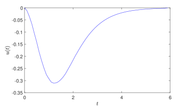
Figure 1: LQ-optimal feedback control at $x=0$ . This control signal minimizes the cost functional (89), and is derived by solving system (66) after discretization.

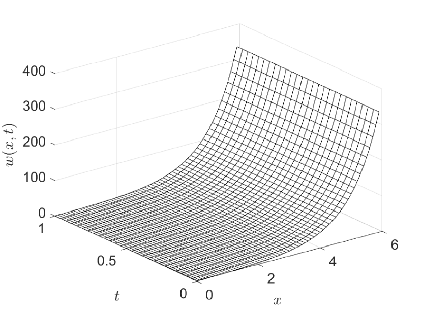
(a) Uncontrolled $w(x,t)$

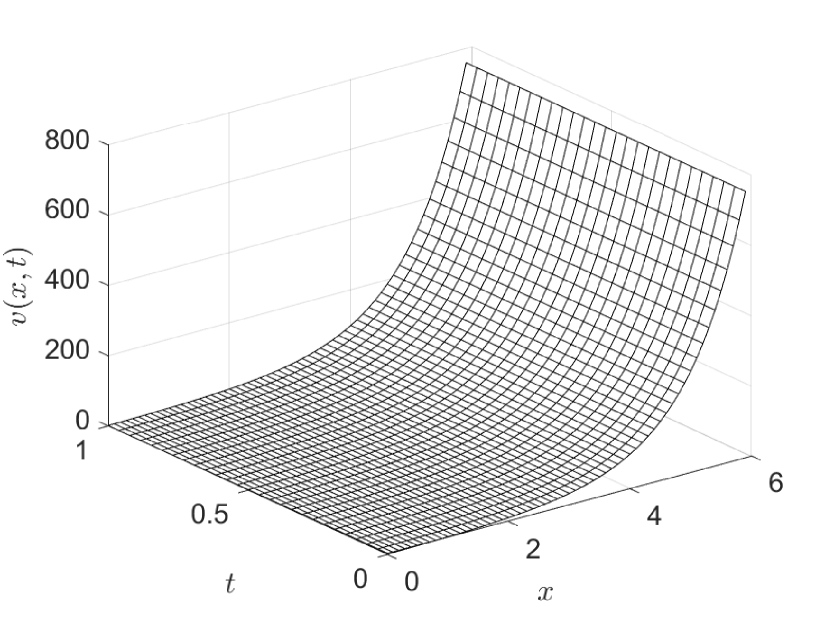
(b) Uncontrolled $v(x,t)$

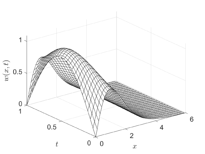
(c) Controlled $w(x,t)$

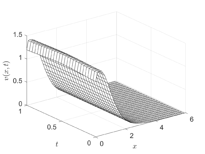
(d) Controlled $v(x,t)$

Figure 2: A 3D landscape of the dynamics of a coupled parabolic-elliptic system with initial condition $w_{0}=\sin(\pi x)$, $v_{0}=\beta(d_{xx}-\gamma I)^{-1}\sin(\pi x)$, without and with control (64). The parameters of the system are $\rho=1$, $\gamma=\alpha=\beta=2.$ The uncontrolled system is unstable, but the use of LQ feedback control causes the states to decay towards zero.

6 Conclusions

This paper extends the classical finite-time linear quadratic control problem for finite-dimensional DAEs into the infinite-dimensional case. We showed the existence of a continuous optimal control that ensures the consistency of the initial conditions while minimizing the cost functional. Decomposing the PDAE into a Weierstra$\beta$ canonical form was crucial in the proofs. However, the optimal control can be calculated derived differential Riccati equation without projecting of any operators other than the state weight. Future work will consider the minimization problem on an infinite-time horizon.

The class of PDAEs considered here was restricted to those with radiality-index zero. We aim to extend the results to higher-index PDAEs in future research. This already been done [3] for finite-dimensional DAEs without the use of behaviors. Another prospective research problem is to examine the linear quadratic control problem for linear PDAEs in situations where the operator associated with the penalization on the $L_{2}$-norm of the control input is not necessarily invertible, since as illustrated in [35] a unique solution can exist for the optimization problem in the finite-dimensional situation. Finally, since the derived differential Riccati equation is an operator equation on an infinite-dimensional Hilbert space, numerical treatment for solving needs further attention.

References

[1]J. Ahn and C. Yoon, Global well-posedness and stability of constant equilibria in parabolic–elliptic chemotaxis systems without gradient sensing, Nonlinearity, 32 (2019), p. 1327.
[2]A. Alalabi and K. A. Morris, Boundary control and observer design via backstepping for a coupled parabolic-elliptic system, preprint, (2023).
[3]A. Alalabi and K. A. Morris, Linear quadratic control problem on a finite-horizon for a class of differential-algebraic equations, in the proceedings of the 2024 American Control Conference, (2024).
[4]A. Bartel and R. Pulch, A concept for classification of partial differential algebraic equations in nanoelectronics, in Progress in Industrial Mathematics at ECMI 2006, Springer, (2008), pp. 506–511.
[5]D. Bender and A. Laub, The linear-quadratic optimal regulator for descriptor systems, IEEE Transactions on Automatic Control, 32 (1987), pp. 672–688.
[6]D. Bender and A. Laub, The linear-quadratic optimal regulator for descriptor systems, IEEE Transactions on Automatic Control, 32 (1987), pp. 672–688.
[7]T. Breiten, K. Kunisch, and L. Pfeiffer, Feedback stabilization of the two-dimensional Navier–Stokes equations by value function approximation, Applied Mathematics & Optimization, 80 (2019), pp. 599–641.
[8]S. L. Campbell and W. Marszalek, The index of an infinite dimensional implicit system, Mathematical and Computer Modelling of Dynamical Systems, 5 (1999), pp. 18–42.
[9]R. Curtain and H. Zwart, Introduction to infinite-dimensional systems theory: a state-space approach, vol. 71, Springer Nature, (2020).
[10]G.-R. Duan, Analysis and design of descriptor linear systems, vol. 23, Springer Science & Business Media, (2010).
[11]M. Erbay, B. Jacob, K. Morris, T. Reis, and C. Tischendorf, Index concepts for linear differential-algebraic equations in finite and infinite dimensions, arXiv preprint arXiv:2401.01771, (2024).
[12]Z. Ge and D. Feng, Well-posed problem of nonlinear singular distributed parameter systems and nonlinear ge-semigroup, Science China Information Sciences, 56 (2013), pp. 1–14.
[13]Z. Ge, X. Ge, and J. Zhang, Approximate controllability and approximate observability of singular distributed parameter systems, IEEE Transactions on Automatic Control, 65 (2019), pp. 2294–2299.
[14]Z. Ge, G. Zhu, and D. Feng, Exact controllability for singular distributed parameter system in hilbert space, Science in China Series F: Information Sciences, 52 (2009), pp. 2045–2052.
[15]H. Gernandt and T. Reis, Linear-quadratic optimal control for abstract differential-algebraic equations, arXiv preprint arXiv:2402.08762, (2024).
[16]G. V. Grenkin, A. Y. Chebotarev, A. E. Kovtanyuk, N. D. Botkin, and K.-H. Hoffmann, Boundary optimal control problem of complex heat transfer model, Journal of Mathematical Analysis and Applications, 433 (2016), pp. 1243–1260.
[17]M. Günther, A joint dae/pde model for interconnected electrical networks, Mathematical and Computer Modelling of Dynamical Systems, 6 (2000), pp. 114–128.
[18]M. Heinkenschloss, D. C. Sorensen, and K. Sun, Balanced truncation model reduction for a class of descriptor systems with application to the oseen equations, SIAM Journal on Scientific Computing, 30 (2008), pp. 1038–1063.
[19]B. Jacob and K. Morris, On solvability of dissipative partial differential-algebraic equations, IEEE Control Systems Letters, 6 (2022), pp. 3188–3193.
[20]E. Kreyszig, Introductory functional analysis with applications, vol. 17, John Wiley & Sons, (1991).
[21]P. Kunkel and V. Mehrmann, Differential-algebraic equations: analysis and numerical solution, vol. 2, European Mathematical Society, (2006).
[22]R. Lamour, R. März, and C. Tischendorf, Differential-algebraic equations: a projector based analysis, Springer Science & Business Media, (2013).
[23]A. W. Leung, Systems of nonlinear partial differential equations: applications to biology and engineering, vol. 49, Springer Science & Business Media, (2013).
[24]P. Lin, A sequential regularization method for time-dependent incompressible navier–stokes equations, SIAM Journal on Numerical Analysis, 34 (1997), pp. 1051–1071.
[25]W. S. Martinson and P. I. Barton, A differentiation index for partial differential-algebraic equations, SIAM Journal on Scientific Computing, 21 (2000), pp. 2295–2315.
[26]V. Mehrmann and H. Zwart, Abstract dissipative hamiltonian differential-algebraic equations are everywhere, arXiv preprint arXiv:2311.03091, (2023).
[27]V. L. Mehrmann, The autonomous linear quadratic control problem: theory and numerical solution, Springer, (1991).
[28]K. A. Morris, Introduction to feedback control, Academic Press, Inc., (2000).
[29]K. A. Morris, Controller design for distributed parameter systems, Springer, (2020).
[30]H. Parada, E. Cerpa, and K. A. Morris, Feedback control of an unstable parabolic-elliptic system with input delay, preprint, (2020).
[31]M. Petreczky and S. Zhuk, Solutions of differential–algebraic equations as outputs of lti systems: Application to LQ control problems, Automatica, 84 (2017), pp. 166–173.
[32]A. A. Polezhaev, R. A. Pashkov, A. I. Lobanov, and I. B. Petrov, Spatial patterns formed by chemotactic bacteria escherichia coli, International Journal of Developmental Biology, 50 (2003), pp. 309–314.
[33]J. Rang and L. Angermann, Perturbation index of linear partial differential-algebraic equations, Applied numerical mathematics, 53 (2005), pp. 437–456.
[34]T. Reis, Controllability and observability of infinite-dimensional descriptor systems, IEEE transactions on automatic control, 53 (2008), pp. 929–940.
[35]T. Reis and M. Voigt, Linear-quadratic optimal control of differential-algebraic systems: the infinite time horizon problem with zero terminal state, SIAM Journal on Control and Optimization, 57 (2019), pp. 1567–1596.
[36]T. Stykel, Balanced truncation model reduction for semidiscretized Stokes equation, Linear Algebra and its Applications, 415 (2006), pp. 262–289.
[37]G. A. Sviridyuk and V. E. Fedorov, Linear Sobolev type equations and degenerate semigroups of operators, de Gruyter, (2003).
[38]Y. Wagner, A further index concept for linear PDAEs of hyperbolic type, Mathematics and computers in simulation, 53 (2000), pp. 287–291.