Robust finite element solvers for distributed hyperbolic optimal control problems

Abstract

We propose, analyze, and test new robust iterative solvers for systems of linear algebraic equations arising from the space-time finite element discretization of reduced optimality systems defining the approximate solution of hyperbolic distributed, tracking-type optimal control problems with both the standard $L^{2}$ and the more general energy regularizations. In contrast to the usual time-stepping approach, we discretize the optimality system by space-time continuous piecewise-linear finite element basis functions which are defined on fully unstructured simplicial meshes. If we aim at the asymptotically best approximation of the given desired state $y_{d}$ by the computed finite element state $y_{\varrho h}$, then the optimal choice of the regularization parameter $\varrho$ is linked to the space-time finite element mesh-size $h$ by the relations $\varrho=h^{4}$ and $\varrho=h^{2}$ for the $L^{2}$ and the energy regularization, respectively. For this setting, we can construct robust (parallel) iterative solvers for the reduced finite element optimality systems. These results can be generalized to variable regularization parameters adapted to the local behavior of the mesh-size that can heavily change in the case of adaptive mesh refinements. The numerical results illustrate the theoretical findings firmly.

Keywords: Hyperbolic optimal control problems, $L^{2}$ regularization, energy regularization, space-time finite element methods, error estimates, adaptivity, solvers 2010 MSC: 49J20, 49M05, 35L05, 65M60, 65M15, 65N22

1 Introduction

Let us first consider abstract optimal control problems (OCPs) of the form: Find the state $y_{\varrho}\in Y$ and the control $u_{\varrho}\in U$ minimizing the cost functional

$$\mathcal{J}(y_{\varrho},u_{\varrho}):=\mathcal{J}_{\varrho}(y_{\varrho},u_{\varrho}):=\frac{1}{2}\,\|y_{\varrho}-y_{d}\|_{H}^{2}+\frac{\varrho}{2}\,\|u_{\varrho}\|_{U}^{2},$$ (1)

subject to the state equation

$$By_{\varrho}=u_{\varrho}\quad\mbox{in}\;\;U\subset P^{*},$$ (2)

where the desired state (target) $y_{d}\in H$ and the regularization parameter $\varrho>0$ are given. We mention that, in optimal control, $\varrho$ also allows to influence the costs of the control in terms of $\|u\|_{U}^{2}$. The state space $Y$, the adjoint state space $P$, the observation space $H$, and the control space $U$ are Hilbert spaces equipped with the corresponding norms and scalar products. We assume that $Y\subset H\subset Y^{*}$ and $P\subset H\subset P^{*}$ are Gelfand triples, where $Y^{*}$ and $P^{*}$ denote the dual spaces of $Y$ and $P$, respectively. The duality products $\langle\cdot,\cdot\rangle:Y^{*}\times Y\to\mathbb{R}$ and $\langle\cdot,\cdot\rangle:P^{*}\times P\to\mathbb{R}$ are assumed to be extensions of the scalar product $\langle\cdot,\cdot\rangle_{H}$ in $H$. The state operator $B$ is usually an isomorphism as mapping from $Y$ to $P^{*}$. So, we are interested to control the state equation (2) not only in $U=H$, where $H=L^{2}$ in the standard setting ($L^{2}$-regularization), but also in $U=P^{*}$ that is sometimes called energy regularization. Such kind of optimal control problems were already studied in the classical monograph [25] by Lions who also admitted additional control constraints. Since then many books and papers on the analysis and numerics of such kind of optimal control problems often with additional inequality constraints imposed on the control $u$ or/and the state $y$ have been published. We here refer the reader only to the books [10, 17, 42], and the recent omnibus volume [15] on optimization and control for partial differential equations (PDEs).

We will here only consider tracking-type, distributed hyperbolic OCPs that are represented by the model state operator $B=\Box=\partial_{tt}-\Delta_{x}$ (wave operator). The reduced optimality system that characterizes the unique solution of the optimal control problem under consideration is discretized by an unstructured simplicial finite element (FE) method that is a real space-time finite element method; see [23, 24] and [26] for the parabolic and hyperbolic cases, respectively. This all-at-once space-time discretization of the reduced optimality system leads to a symmetric, but indefinite (SID) system of FE equations of the form

$$\begin{bmatrix}A_{\varrho h}&B_{h}\\ B_{h}^{\top}&-M_{h}\end{bmatrix}\begin{bmatrix}\mathbf{p}_{h}\\ \mathbf{y}_{h}\\ \end{bmatrix}=\begin{bmatrix}\mathbf{0}_{h}\\ -\mathbf{y}_{dh}\\ \end{bmatrix}.$$ (3)

as in the elliptic case, where the matrix $B_{h}$ is the FE representation of the state operator $B$, $M_{h}$ is nothing but the mass matrix, $A_{\varrho h}$ represents the regularization term, and the subscript $h$ is a suitable discretization parameter. In the standard case of $L^{2}$ regularization with a constant regularization (cost) parameter $\varrho$, the matrix $A_{\varrho h}$ equals $\varrho^{-1}\overline{M}_{h}$, where $\overline{M}_{h}$ is the mass matrix from the finite element space for the approximation of the adjoint state $p$. The matrices $M_{h}$ and $A_{\varrho h}$ are symmetric and positive definite (SPD). In contrast to this approach to time-dependent optimal control problems, the standard time-stepping discretization combined with a FE space discretization produces smaller systems of the form (3) at each time step; see, e.g., [19, 31], and the references therein.

There is a huge amount of publications on preconditioners and iterative solvers for general systems of algebraic equations with symmetric and indefinite system matrices such as (3). We refer the reader to the survey papers [6, 43], the books [5, 12, 32], the review paper [27], and the references therein for a comprehensive overview on saddle point solvers in general. In particular, there are many papers devoted to the efficient solution of SID systems arising from PDE-constrained OCPs with the standard $L^{2}$ regularization and fixed regularization parameter $\varrho$. More recently, preconditioners leading to $\varrho$-robust iterative solvers have been developed for PDE-constrained OCPs subject to different state equations without and with control and/or state constraints; see, e.g., [1, 2, 4, 11, 29, 30, 34, 35, 36, 41] and the references provided in these papers.

In this paper, we first investigate the deviation of the exact state $y_{\varrho}$ from the desired state $y_{d}$ with respect to (wrt) the $H=L^{2}(Q)$ norm in dependence on the regularization parameter $\varrho$ and the regularity of the desired state $y_{d}$. It turns out that the quantitative behavior is practically the same as was first proved for elliptic optimal control problems with both $L^{2}$ and energy regularization in [28]. After the simplicial space-time finite element (FE) discretization, we choose $\varrho$ in such a way that the finite element state $y_{\varrho h}$, corresponding to the nodal vector $\mathbf{y}_{h}$ as part of the solution of (3), provides an asymptotically optimal approximation to the desired state $y_{d}$ in the $L^{2}$ norm. It was already shown in [26] that $\varrho=h^{2}$ is always the optimal choice in the case of the energy regularization independent of the regularity of the desired state $y_{d}$. In this paper, we also investigate the standard $L^{2}$ regularization for which we get $\varrho=h^{4}$ as optimal choice. These choices of $\varrho$ provide not only an optimal balance between the regularization and discretization errors, but also a well-conditioned primal Schur Complement (SC) $S_{\varrho h}=B_{h}^{\top}A_{\varrho h}^{-1}B_{h}+M_{h}$ of the system matrix in the SID system (3). More precisely, we show that the Schur complement $S_{\varrho h}$ is spectrally equivalent to the mass matrix $M_{h}$ and, therefore, to the diagonal lumped mass matrix $D_{h}=\text{lump}(M_{h})$ with computable spectral equivalence constants. This result is crucial for the construction of fast iterative solvers for the reduced algebraic optimality system (3). It turns out that the Schur-Complement Preconditioned Conjugate Gradient (SC-PCG) method for solving the SPD SC problem

$$S_{\varrho h}\mathbf{y}_{h}=\mathbf{y}_{dh},$$ (4)

which arises from (3) by eliminating the adjoint FE state $\mathbf{p}_{h}$ from (3), is an efficient alternative to the solution of the SID system (3) by means of the closely related Bramble-Pasciak PCG (BP-PCG) [8], especially, in the case of the $L^{2}$ regularization when $A_{\varrho h}^{-1}$ can be replaced by $(\text{lump}(\overline{M}_{\varrho h}))^{-1}$ ensuring a fast matrix-by-vector multiplication. We note that these results remain valid for the corresponding variable choice of the regularization parameter $\varrho$ adapted to the local behavior of the size of the simplicial space-time mesh that can heavily vary in the case of adaptive FE discretisations as used in some of our numerical experiments.

The remainder of the paper is organized as follows: In Section 2, we introduce some preliminary material, and specify the hyperbolic OCPs that we are going to investigate. More precisely, we consider the standard $L^{2}$ regularization and the more general energy regularization. The space-time finite element discretization of these hyperbolic OCPs on unstructured simplicial meshes is presented and analyzed in Section 3. Section 4 is devoted to efficient iterative methods for solving the algebraic systems arising from the space-time finite element discretization of the reduced optimality systems. In Section 5, we present and discuss our numerical results. Finally, we draw some conclusions and give an outlook in Section 6.

2 Preliminaries and specifications

As a model problem, we consider a distributed optimal control problem subject to the wave equation with homogeneous Dirichlet boundary and initial conditions. Therefore, let $\Omega\subset{\mathbb{R}}^{d}$, $d=1,2,3$, be a bounded spatial domain with, for $d=2,3$, Lipschitz boundary $\Gamma=\partial\Omega$, and let $0<T<\infty$ be a given finite time horizon. Further we introduce the space-time cylinder $Q:=\Omega\times(0,T)$, its lateral boundary $\Sigma:=\Gamma\times(0,T)$, its bottom $\Sigma_{0}:=\Omega\times\{0\}$, and its top $\Sigma_{T}:=\Omega\times\{T\}$. For a given target $y_{d}\in L^{2}(Q)$ and a regularization parameter $\varrho>0$, we consider the minimization of the cost functional (1) with $H=L^{2}(Q)$, subject to the homogeneous initial-boundary value problem for the wave equation

$$\Box y_{\varrho}:=\partial_{tt}y_{\varrho}-\Delta_{x}y_{\varrho}=u_{\varrho}\;\mbox{in}\,Q,\;y_{\varrho}=0\;\mbox{on}\,\Sigma,\;y_{\varrho}=\partial_{t}y_{\varrho}=0\;\mbox{on}\,\Sigma_{0}.$$ (5)

In order to derive a variational formulation of the wave equation (5), we introduce

$$H_{0;0,}^{1,1}(Q) :=\{y\in L^{2}(Q):\nabla_{x}y\in[L^{2}(Q)]^{d},\partial_{t}y\in L^{2}(Q),y=0\,\text{on}\,\Sigma,y=0\,\text{on}\,\Sigma_{0}\},$$

$$H_{0;,0}^{1,1}(Q) :=\{q\in L^{2}(Q):\nabla_{x}q\in[L^{2}(Q)]^{d},\partial_{t}q\in L^{2}(Q),q=0\,\text{on}\,\Sigma,q=0\,\text{on}\,\Sigma_{T}\},$$

both equipped with the norm $|v|_{H^{1}(Q)}=(\|\partial_{t}v\|_{L^{2}(Q)}^{2}+\|\nabla_{x}v\|_{L^{2}(Q)}^{2})^{1/2}$. Note that $y\in H^{1,1}_{0;0,}(Q)$ covers zero initial conditions $y(x,0)=0$, while, for $q\in H^{1,1}_{0;,0}(Q)$, we have $q(x,T)=0$, $x\in\Omega$. We now consider the variational formulation of (5) to find $y_{\varrho}\in H^{1,1}_{0;0,}(Q)$ such that

$$b(y_{\varrho},q):=-\langle\partial_{t}y_{\varrho},\partial_{t}q\rangle_{L^{2}(Q)}+\langle\nabla_{x}y_{\varrho},\nabla_{x}q\rangle_{L^{2}(Q)}=\langle u_{\varrho},q\rangle_{L^{2}(Q)}$$ (6)

is satisfied for all $q\in H^{1,1}_{0;,0}(Q)$. Unique solvability of (6) follows when assuming $u_{\varrho}\in L^{2}(Q)$, see, e.g., [20, 38]. This motivates to consider the optimal control problem with $L^{2}$ regularization first.

2.1 The $L^{2}$ regularization $U=L^{2}(Q)$

Let us first consider the more common $L^{2}$ regularization with $U=L^{2}(Q)$. Then, for any $u_{\varrho}\in L^{2}(Q)$, the variational formulation (6) admits a unique solution $y_{\varrho}\in H_{0;0,}^{1,1}(Q)$ satisfying the stability estimate

$$\|y_{\varrho}\|_{H_{0;0,}^{1,1}(Q)}\leq\frac{T}{\sqrt{2}}\,\|u_{\varrho}\|_{L^{2}(Q)},$$

see, e.g., [20, Theorem 5.1, p. 169], or [38, Theorem 5.1]. Thus, we can define the solution operator $y_{\varrho}=\mathcal{S}u_{\varrho}$ with $\mathcal{S}:L^{2}(Q)\to H_{0;0,}^{1,1}(Q)$, and we can consider the reduced cost functional

$$\widehat{\mathcal{J}}(u_{\varrho})=\frac{1}{2}\,\|\mathcal{S}u_{\varrho}-y_{d}\|_{L^{2}(Q)}^{2}+\frac{1}{2}\,\varrho\,\|u_{\varrho}\|_{L^{2}(Q)}^{2},$$

for which the minimizer satisfies the gradient equation

$$\mathcal{S}^{\ast}(\mathcal{S}u_{\varrho}-y_{d})+\varrho\,u_{\varrho}=0\quad\text{in}\;L^{2}(Q).$$ (7)

When introducing the adjoint state $p_{\varrho}:=\mathcal{S}^{\ast}(\mathcal{S}u_{\varrho}-y_{d})\in P=H_{0;,0}^{1,1}(Q)$ as the unique weak solution of the adjoint problem

$$\partial_{tt}p_{\varrho}-\Delta_{x}p_{\varrho}=y_{\varrho}-y_{d}\;\mbox{in}\,Q,\;p_{\varrho}=0\;\mbox{on}\,\Sigma,\;p_{\varrho}=\partial_{t}p_{\varrho}=0\;\mbox{on}\,\Sigma_{T},$$ (8)

we end up with the optimality system, including the forward problem (5), the adjoint problem (8), and the gradient equation (7).

Remark 1.

We note that, by the gradient equation (7), we have

$$u_{\varrho}=-\varrho^{-1}\,p_{\varrho}\in H_{0;,0}^{1,1}(Q).$$ (9)

Thus, actually the control $u_{\varrho}\in H^{1,1}_{0;,0}(Q)$ is more regular, but also inherits, probably unpleasant, boundary and terminal conditions from the adjoint state.

When eliminating the control $u_{\varrho}=\Box y_{\varrho}$, from (5), we get by the gradient equation that $p_{\varrho}+\varrho\,\Box y_{\varrho}=0$, and the reduced optimality system in variational form is to find $(p_{\varrho},y_{\varrho})\in H_{0;,0}^{1,1}(Q)\times H_{0;0,}^{1,1}(Q)$ such that

$$\begin{array}[]{rcrcll}\varrho^{-1}\,\langle p_{\varrho},q\rangle_{L^{2}(Q)}&+&b(y_{\varrho},q)&=&0&\forall\,q\in H_{0;,0}^{1,1}(Q),\\[5.69054pt] -b(z,p_{\varrho})&+&\langle y_{\varrho},z\rangle_{L^{2}(Q)}&=&\langle y_{d},z\rangle_{L^{2}(Q)}&\forall\,z\in H_{0;0,}^{1,1}(Q).\end{array}$$ (10)

Unique solvability of (10) follows from the way we derived the system.

Remark 2.

In addition, we can eliminate the adjoint variable $p_{\varrho}=-\varrho\,u_{\varrho}=-\varrho\,\Box y_{\varrho}$ in the adjoint equation (8) to conclude

$$\varrho\,\Box^{2}y_{\varrho}=-\Box p_{\varrho}=y_{d}-y_{\varrho},$$

and, therefore, we get

$$\begin{array}[]{rcrclcl}\lx@intercol\hfil\varrho\,\Box^{2}y_{\varrho}+y_{\varrho}\lx@intercol&=&y_{d}&&\mbox{in}\;Q,\\[2.84526pt] &&y_{\varrho}=\Box\,y_{\varrho}&=&0&&\mbox{on}\;\Sigma,\\[2.84526pt] &&y_{\varrho}=\partial_{t}y_{\varrho}&=&0&&\mbox{on}\;\Sigma_{0},\\[2.84526pt] &&\Box\,y_{\varrho}=\partial_{t}\Box\,y_{\varrho}&=&0&&\mbox{on}\;\Sigma_{T},\end{array}$$ (11)

which is nothing but a kind of bi-wave equation with boundary and terminal conditions inherited from the adjoint state $p_{\varrho}$.

As a last step, we present some estimates for the distance $\|y_{\varrho}-y_{d}\|_{L^{2}(Q)}$ of the regularized state $y_{\varrho}$ from the target $y_{d}$, which only depends on the regularization parameter $\varrho$, and on the regularity of the target.

Lemma 1.

Let $y_{d}\in L^{2}(Q)$. For the unique solution $(p_{\varrho},y_{\varrho})\in H_{0;,0}^{1,1}(Q)\times H_{0;0,}^{1,1}(Q)$ of (10) there holds

$$\|y_{\varrho}-y_{d}\|_{L^{2}(Q)}\leq\|y_{d}\|_{L^{2}(Q)}.$$ (12)

If in addition $y_{d}\in H_{0;0,}^{1,1}(Q)$ such that $\Box y_{d}\in L^{2}(Q)$, then

$$\|y_{\varrho}-y_{d}\|_{L^{2}(Q)}\leq\sqrt{\varrho}\,\|\Box y_{d}\|_{L^{2}(Q)}.$$ (13)

Moreover, we also have

$$\|\Box y_{\varrho}\|_{L^{2}(Q)}\leq\|\Box y_{d}\|_{L^{2}(Q)}.$$ (14)

Proof.

Firstly, let $y_{d}\in L^{2}(Q)$. Testing (10) with $q=p_{\varrho}$ and $z=y_{\varrho}$, we obtain

$$\langle y_{\varrho}-y_{d},y_{\varrho}\rangle_{L^{2}(Q)}=b(y_{\varrho},p_{\varrho})=-\varrho^{-1}\,\|p_{\varrho}\|_{L^{2}(Q)}^{2},$$

from which we further deduce, using a Cauchy–Schwarz inequality, that

$$\|y_{\varrho}-y_{d}\|_{L^{2}(Q)}^{2}+\varrho^{-1}\,\|p_{\varrho}\|_{L^{2}(Q)}^{2}=\langle y_{d}-y_{\varrho},y_{d}\rangle_{L^{2}(Q)}\leq\|y_{\varrho}-y_{d}\|_{L^{2}(Q)}\|y_{d}\|_{L^{2}(Q)},$$

which gives (12). If now $y_{d}\in H_{0;0,}^{1,1}(Q)$ such that $\Box y_{d}\in L^{2}(Q)$, we can test (10) with $z=y_{d}-y_{\varrho}$, and using the relations (5) and (7), i.e., $p_{\varrho}=-\varrho\,\Box y_{\varrho}$, we get

$$\|y_{d}-y_{\varrho}\|_{L^{2}(Q)}^{2} = \langle y_{d}-y_{\varrho},y_{d}-y_{\varrho}\rangle_{L^{2}(Q)}=b(y_{\varrho}-y_{d},p_{\varrho})=b(y_{\varrho},p_{\varrho})-b(y_{d},p_{\varrho})$$

$$= -\varrho\,\langle\Box y_{\varrho},\Box y_{\varrho}\rangle_{L^{2}(Q)}+\varrho\,\langle\Box y_{d},\Box y_{\varrho}\rangle_{L^{2}(Q)}.$$

Reordering and applying a Cauchy–Schwarz inequality, this gives

$$\|y_{d}-y_{\varrho}\|_{L^{2}(Q)}^{2}+\varrho\,\|\Box y_{\varrho}\|_{L^{2}(Q)}^{2}=\varrho\,\langle\Box y_{d},\Box y_{\varrho}\rangle_{L^{2}(Q)}\leq\varrho\,\|\Box y_{d}\|_{L^{2}(Q)}\|\Box y_{\varrho}\|_{L^{2}(Q)},$$

from which (14) and (13) follow. ∎

Corollary 1.

From the gradient equation (9), the primal wave equation in (5), and (14), we conclude

$$\|p_{\varrho}\|_{L^{2}(Q)}=\varrho\,\|u_{\varrho}\|_{L^{2}(Q)}=\varrho\,\|\Box y_{\varrho}\|_{L^{2}(Q)}\leq\varrho\,\|\Box y_{d}\|_{L^{2}(Q)},$$ (15)

while from the wave equation in (8) and using (13), this gives

$$\|\Box p_{\varrho}\|_{L^{2}(Q)}=\|y_{\varrho}-y_{d}\|_{L^{2}(Q)}\leq\sqrt{\varrho}\,\|\Box y_{d}\|_{L^{2}(Q)}.$$ (16)

Proposition 1.

The error estimates (13) and (14) as well as (15) and (16) may motivate the use of a space interpolation argument in order to derive related error estimates in $H^{1}(Q)$. Unfortunately, this does not hold true in general. At this point, we therefore assume that the given data are such that the following regularization error estimates hold true, i.e.,

$$|y_{\varrho}-y_{d}|_{H^{1}(Q)}\leq c\,\varrho^{1/4}\,\|\Box y_{d}\|_{L^{2}(Q)},$$ (17)

and

$$|p_{\varrho}|_{H^{1}(Q)}\leq c\,\varrho^{3/4}\,\|\Box y_{d}\|_{L^{2}(Q)}.$$ (18)

All our numerical experiments performed for smooth targets confirm the estimates (17) and (18); see Appendix.

Remark 3.

The regularization error estimates (17) and (18) are a simple consequence of the space interpolation type estimate

$$\|v\|^{2}_{H^{1}(Q)}\leq c\,\|\Box v\|_{L^{2}(Q)}\|v\|_{L^{2}(Q)}$$ (19)

for all $v\in H^{1}(Q)$ with $\Box v\in L^{2}(Q)$ and $v=\partial_{t}v=0$ on $\Sigma_{0}$. In order to prove (19) we can use the normalized eigenfunctions $\phi_{k}\in H^{1}_{0}(\Omega)$ with eigenvalues $\mu_{k}$ of the spatial Dirichlet eigenvalue problem for the Laplacian to write

$$v(x,t)=\sum\limits_{k=1}^{\infty}V_{k}(t)\phi_{k}(x)\,,\quad V_{k}(0)=V_{k}^{\prime}(0)=0,$$

and it turns out that (19) is a consequence of the estimate

$$\|V_{k}^{\prime}\|^{2}_{L^{2}(0,T)}+\mu_{k}\,\|V_{k}\|^{2}_{L^{2}(0,T)}\leq c\,\|V_{k}^{\prime\prime}+\mu_{k}\,V_{k}\|_{L^{2}(0,T)}\|V_{k}\|_{L^{2}(0,T)},\;k\in{\mathbb{N}}.$$ (20)

In particular, for, see [44, Theorem 4.2.6],

$$V_{k}(t):=\frac{1}{\sqrt{T^{3}}}\int_{0}^{t}s\,\sin(\sqrt{\mu_{k}}s)\,ds\quad\mbox{for}\;t\in[0,T]$$

we conclude $c^{-1}=\mathcal{O}(\sqrt{1/\mu_{k}})$, and thus $c\to\infty$ as $k\to\infty$. Hence, this analysis indicates that the regularization error estimates (17) and (18) are only violated when high-oscillating contributions appear.

2.2 The energy regularization in $U=P^{\ast}=[H_{0;,0}^{1,1}(Q)]^{\ast}$

We note that so far we needed $u_{\varrho}\in L^{2}(Q)$ to admit a unique solution of the variational formulation (6). As we test (6) with functions $q\in P=H_{0;,0}^{1,1}(Q)$, a natural question to appear is, whether we can also choose the control in the dual space $u_{\varrho}\in P^{\ast}=[H_{0;,0}^{1,1}(Q)]^{\ast}$. But, as it turns out, the operator $B:H_{0;0,}^{1,1}(Q)\to P^{\ast}$ as implied by the bilinear form $b(y,q)=\langle By,q\rangle_{Q}$ for all $y\in H^{1,1}_{0;0,}(Q)$ and for all $q\in H^{1,1}_{0;,0}(Q)$ does not define an isomorphism, see [39, Theorem 1.1]. Recapitulating the work of [39], see also [26], we will define suitable spaces, such that the wave operator is an isomorphism. The first issue to overcome is the establishment of an inf-sup condition, guaranteeing the injectivity of the operator. It fails to hold in the above setting, since the initial condition $\partial_{t}y_{\varrho}(x,t)\big{|}_{t=0}$ enters the variational formulation naturally, which is not appropriate in this case. In order to incorporate it in a meaningful sense, we will modify the state space. Let $Q_{-}:=\Omega\times(-T,T)$ denote the enlarged space-time domain, and define the zero extension of a function $y\in L^{2}(Q)$ by

$$\widetilde{y}(x,t):=\begin{cases}y(x,t)&\mbox{for}\;(x,t)\in Q,\\ 0,&\mbox{else.}\end{cases}$$

Then, we consider the application of the wave operator in a distributional sense, i.e., for all $\varphi\in C_{0}^{\infty}(Q_{-})$ we define

$$\langle\Box\widetilde{y},\varphi\rangle_{Q_{-}}:=\int_{Q_{-}}\widetilde{y}(x,t)\,\Box\varphi(x,t)\,dx\,dt=\int_{Q}y(x,t)\,\Box\varphi(x,t)\,dx\,dt.$$

Using this definition, we can introduce the space

$$\mathcal{H}(Q):=\Big{\{}y=\widetilde{y}_{|_{Q}}:\widetilde{y}\in L^{2}(Q_{-}),\;\widetilde{y}_{|\Omega\times(-T,0)}=0,\;\Box\widetilde{y}\in[H_{0}^{1}(Q_{-})]^{*}\Big{\}},$$

with the graph norm $\|y\|_{\mathcal{H}(Q)}:=(\|y\|_{L^{2}(Q)}^{2}+\|\Box\widetilde{y}\|_{[H_{0}^{1}(Q_{-})]^{*}}^{2})^{1/2}$. The normed vector space $(\mathcal{H}(Q),\|\cdot\|_{\mathcal{H}(Q)})$ is a Banach space, with $H_{0;0,}^{1,1}(Q)\subset\mathcal{H}(Q)$; see [39, Lemma 3.5]. Therefore, we can introduce the space

$$Y:=\mathcal{H}_{0;0,}(Q):=\overline{H_{0;0,}^{1,1}(Q)}^{\|\cdot\|_{\mathcal{H}(Q)}}\subset\mathcal{H}(Q),$$

which will serve as state space. For $y\in Y$, an equivalent norm is given by

$$\|y\|_{Y}=\|\Box\widetilde{y}\|_{[H^{1}_{0}(Q_{-})]^{*}},$$

see [39, Lemma 3.6]. It turns out that $B:{\mathcal{H}}_{0;0,}(Q)\to[H^{1,1}_{0;,0}(Q)]^{\ast}$ defined by $\langle By,q\rangle_{Q}=\langle\Box\widetilde{y},{\mathcal{E}}q\rangle_{Q_{-}}$ for all $(y,q)\in{\mathcal{H}}_{0;0,}(Q)\times H^{1,1}_{0;,0}(Q)$, and using some bounded extension ${\mathcal{E}}:H^{1,1}_{0;,0}(Q)\to H^{1}_{0}(Q_{-})$, e.g., reflection in time, is an isomorphism; see [39, Lemma 3.5, Theorem 3.9]. Moreover, we have

$$\langle\Box\widetilde{y},{\mathcal{E}}q\rangle_{Q_{-}}=-\langle\partial_{t}y,\partial_{t}q\rangle_{L^{2}(Q)}+\langle\nabla_{x}y,\nabla_{x}q\rangle_{L^{2}(Q)}$$ (21)

for $y\in H^{1,1}_{0;0,}(Q)$ and $q\in H^{1,1}_{0;,0}(Q)$, which in particular applies when considering conforming space-time finite element spaces $Y_{h}\subset H^{1,1}_{0;0,}(Q)\subset Y$, and $P_{h}\subset H^{1,1}_{0;,0}(Q)$.

For any given $u_{\varrho}\in P^{\ast}=[H^{1,1}_{0;,0}(Q)]^{\ast}$, we now find a unique $y_{\varrho}\in Y={\mathcal{H}}_{0;0,}(Q)$ satisfying

$$\langle By_{\varrho},q\rangle_{Q}=\langle\Box\widetilde{y}_{\varrho},{\mathcal{E}}q\rangle_{Q_{-}}=\langle u_{\varrho},q\rangle_{Q}\quad\mbox{for all}\;q\in H^{1,1}_{0;,0}(Q).$$ (22)

Thus, we might consider the reduced cost functional

$$\widetilde{\mathcal{J}}(y_{\varrho})=\frac{1}{2}\,\|y_{\varrho}-y_{d}\|_{L^{2}(Q)}^{2}+\frac{\varrho}{2}\,\|By_{\varrho}\|_{P^{\ast}}^{2}.$$ (23)

To realize the norm of the dual space $P^{\ast}$, we make use of the following auxiliary Riesz operator $A:P\to P^{\ast}$ defined by

$$\langle Ap,q\rangle_{Q}:=\langle\partial_{t}p,\partial_{t}q\rangle_{L^{2}(Q)}+\langle\nabla_{x}p,\nabla_{x}q\rangle_{L^{2}(Q)}\quad\text{for all }p,q\in P;$$ (24)

see also [26]. With this, the reduced cost functional becomes

$$\widetilde{\mathcal{J}}(y_{\varrho})=\frac{1}{2}\,\langle y_{\varrho}-y_{d},y_{\varrho}-y_{d}\rangle_{L^{2}(Q)}+\frac{\varrho}{2}\,\langle A^{-1}By_{\varrho},By_{\varrho}\rangle_{Q},$$

for which the minimizer is characterized as the solution $y_{\varrho}\in Y$ of the gradient equation

$$\varrho\,B^{\ast}A^{-1}By_{\varrho}+y_{\varrho}=y_{d}\quad\text{in }Y^{\ast}.$$ (25)

Note that the operator $S:=B^{\ast}A^{-1}B:Y\to Y^{\ast}$ is an isomorphism, since $A:P\to P^{\ast}$, and $B:Y\to P^{\ast}$ are isomorphic and therefore, (25) admits a unique solution. In particular, see [26, Lemma 3.1], $S:Y\to Y^{\ast}$ is bounded, self-adjoint, and $Y$-elliptic, and thus defines an equivalent norm

$$\|y\|_{Y}\leq\|y\|_{S}:=\sqrt{\langle Sy,y\rangle_{Q}}\leq 2\,\|y\|_{Y}\quad\text{for all }y\in Y.$$ (26)

Depending on the regularity of the target $y_{d}$ and on the regularization parameter $\varrho>0$, we can show the following regularization error estimates.

Lemma 2 ([26, Theorem 3.2]).

Let $y_{d}\in L^{2}(Q)$ be given. For the unique solution $y_{\varrho}\in Y$ of (25) there holds

$$\|y_{\varrho}-y_{d}\|_{L^{2}(Q)}\leq\|y_{d}\|_{L^{2}(Q)}.$$ (27)

Further, if $y_{d}\in Y$, then

$$\|y_{\varrho}-y_{d}\|_{L^{2}(Q)}\leq\sqrt{\varrho}\,\|y_{d}\|_{S},\quad\text{and}\quad\|y_{\varrho}-y_{d}\|_{S}\leq\|y_{d}\|_{S}.$$ (28)

Moreover, it holds

$$\|y_{\varrho}\|_{S}\leq\|y_{d}\|_{S}.$$ (29)

At last, if $y_{d}\in Y$ such that $Sy_{d}\in L^{2}(Q)$, then it holds

$$\|y_{\varrho}-y_{d}\|_{L^{2}(Q)}\leq\varrho\,\|Sy_{d}\|_{L^{2}(Q)},\quad\text{and}\quad\|y_{\varrho}-y_{d}\|_{S}\leq\sqrt{\varrho}\,\|Sy_{d}\|_{L_{2}(Q)},$$ (30)

as well as

$$\|Sy_{\varrho}\|_{L^{2}(Q)}\leq\|Sy_{d}\|_{L^{2}(Q)}.$$ (31)

From the above results, and using a space interpolation argument, we conclude the following estimate, see [26, Corollary 3.3]: Let $y_{d}\in H^{s,s}_{0;0,}(Q):=[H^{1,1}_{0;0,}(Q),L^{2}(Q)]_{s}$, for $s\in[0,1]$, or $y_{d}\in H^{s}(Q)\cap H^{1,1}_{0;0,}(Q)$ such that $Sy_{d}\in H^{s-2}(Q)$ for $s\in[1,2]$. Then,

$$\|y_{d}-y_{\varrho}\|_{L^{2}(Q)}\leq c\,\varrho^{s/2}\,\|y_{d}\|_{H^{s}(Q)},\quad s\in[0,2].$$ (32)

Remark 4.

The operator $A=-\Delta_{(x,t)}:P=H_{0;,0}^{1,1}(Q)\to P^{\ast}$ corresponds to the space-time Laplacian with mixed Dirichlet and Neumann boundary conditions. Therefore, the solution $p\in P$ of $Ap=u$ in $Q$ admits the regularity $p\in H^{r+1}(Q)\cap P$ for given $u\in H^{r-1}(Q)$, and some $0\leq r\leq 1$, depending on the geometry of the space-time domain, see, e.g., [9, 14]. In particular, for $y_{d}\in H^{2}(Q)\cap H_{0;0,}^{1,1}(Q)$ it holds that $By_{d}\in L^{2}(Q)$. But, we can in general not guarantee that $A^{-1}By_{d}\in H^{2}(Q)$, and subsequently, $Sy_{d}=B^{\ast}A^{-1}By_{d}\in L^{2}(Q)$ does not need to hold true. This loss of regularity might lead to lower convergence rates in the numerical examples.

Remark 5.

Instead of $Y=\mathcal{H}_{0;0,}(Q)$ and $P^{\ast}=[H_{0;,0}^{1,1}(Q)]^{\ast}$ we might as well consider the strong formulation of the wave equation with $P^{\ast}=L^{2}(Q)$, and a suitable ansatz space $\mathcal{Y}\subset H^{1,1}_{0;,0}(Q)$ such that the wave operator $B:\mathcal{Y}\to L^{2}(Q)$ is an isomorphism, see [44, Section 4.3]. Then, choosing $A:=\operatorname{id}:L^{2}(Q)\to L^{2}(Q)$, we can redo the above steps, deriving the optimality equation (25) with a bounded, self-adjoint, and elliptic operator $S:=B^{\ast}B:\mathcal{Y}\to\mathcal{Y}^{\ast}$, and related regularization error estimates depending on the regularity of the target, and on the parameter $\varrho>0$. In particular, the $L^{2}$ regularization corresponds to the concept of the energy regularization, if we consider the wave operator in a strong form.

3 Space-time finite element discretization

From now on, let us assume that $\Omega\subset\mathbb{R}^{d}$ is either polygonally ($d=2$) or polyhedrally ($d=3$) bounded. Let $\mathcal{T}_{h}=\{\tau_{\ell}\}_{\ell=1}^{N}$ be an admissible, globally quasi-uniform decomposition of $Q$ into shape regular simplicial finite elements $\tau_{\ell}\subset\mathbb{R}^{d+1}$ of mesh size $h_{\ell}=|\tau_{\ell}|^{1/(d+1)}$, $\ell=1,\ldots,N$. Further, let $h=\max_{\ell=1,\ldots,N}h_{\ell}$ denote the maximal mesh size. For the Galerkin discretization of the above derived optimality equations, we introduce conforming finite element spaces of, e.g., piecewise linear and continuous basis functions,

$$Y_{h}=\text{span}\{\varphi_{k}\}_{k=1}^{n_{h}}=S_{h}^{1}(\mathcal{T}_{h})\cap H^{1.1}_{0;0,}(Q)\subset Y=\mathcal{H}_{0;0,}(Q),$$

and

$$P_{h}=\text{span}\{\psi_{i}\}_{i=1}^{m_{h}}=S_{h}^{1}(\mathcal{T}_{h})\cap H^{1.1}_{0;,0}(Q)\subset P=H_{0;,0}^{1,1}(Q).$$

In the following, we will formulate discrete variational formulations for the optimality systems, and derive related error estimates, which will enable us to link the regularization parameter $\varrho$ to the mesh size $h$, revealing an asymptotically optimal choice $\varrho=h^{4}$, and $\varrho=h^{2}$, in the case of the $L^{2}$ regularization and the energy regularization in $P^{\ast}$, respectively.

3.1 The $L^{2}$ regularization $U=L^{2}(Q)$

In order to derive error estimates, it will be useful to first apply the transformation $p_{\varrho}=\sqrt{\varrho}\,\widetilde{p}_{\varrho}$. Then, (10) becomes: find $(\widetilde{p}_{\varrho},y_{\varrho})\in P\times H_{0;0,}^{1,1}(Q)$ such that

$$\begin{array}[]{rcrcll}\displaystyle\frac{1}{\sqrt{\varrho}}\,\langle\widetilde{p}_{\varrho},q\rangle_{L^{2}(Q)}&+&b(y_{\varrho},q)&=&0,&\forall q\in P,\\[5.69054pt] -b(z,\widetilde{p}_{\varrho})&+&\displaystyle\frac{1}{\sqrt{\varrho}}\,\langle y_{\varrho},z\rangle_{L^{2}(Q)}&=&\displaystyle\frac{1}{\sqrt{\varrho}}\,\langle y_{d},z\rangle_{L^{2}(Q)},&\forall z\in H_{0;0,}^{1,1}(Q).\end{array}$$ (33)

The Galerkin variational formulation is then to find $(\widetilde{p}_{\varrho h},y_{\varrho h})\in P_{h}\times Y_{h}$ such that

$$\begin{array}[]{rcrcll}\displaystyle\frac{1}{\sqrt{\varrho}}\,\langle\widetilde{p}_{\varrho h},q_{h}\rangle_{L^{2}(Q)}&+&b(y_{\varrho h},q_{h})&=&0,&\forall q_{h}\in P_{h},\\[5.69054pt] -b(z_{h},\widetilde{p}_{\varrho h})&+&\displaystyle\frac{1}{\sqrt{\varrho}}\,\langle y_{\varrho h},z_{h}\rangle_{L^{2}(Q)}&=&\displaystyle\frac{1}{\sqrt{\varrho}}\,\langle y_{d},z_{h}\rangle_{L^{2}(Q)},&\forall z_{h}\in Y_{h}.\end{array}$$ (34)

Lemma 3.

For any $y_{d}\in L^{2}(Q)$, the Galerkin formulation (34) admits a unique solution $(\widetilde{p}_{\varrho h},y_{\varrho h})\in P_{h}\times Y_{h}$.

Proof.

Testing (34) with $q_{h}=\widetilde{p}_{\varrho h}$, and with $z_{h}=y_{\varrho h}$, and summing up both equations, we get

$$\|\widetilde{p}_{\varrho h}\|_{L^{2}(Q)}^{2}+\|y_{\varrho h}\|_{L^{2}(Q)}^{2}=\langle y_{d},y_{\varrho h}\rangle_{L^{2}(Q)}.$$

Thus, for the homogeneous case $y_{d}=0$, we see that $\widetilde{p}_{\varrho h}=y_{\varrho h}=0$, which yields uniqueness for the solution of the linear problem. Moreover, in the finite dimensional case, uniqueness implies existence. ∎

Lemma 4.

Assume the global inverse inequality

$$|v_{h}|_{H^{1}(Q)}\leq c_{\text{\tiny inv}}\,h^{-1}\,\|v_{h}\|_{L^{2}(Q)}\quad\text{for all }v_{h}\in S_{h}^{1}(\mathcal{T}_{h}).$$ (35)

If we choose $\varrho=h^{4}$, then

$$h^{-2}\|\widetilde{p}_{\varrho}-\widetilde{p}_{\varrho h}\|_{L^{2}(Q)}^{2}+|\widetilde{p}_{\varrho}-\widetilde{p}_{\varrho h}|_{H^{1}(Q)}^{2}+h^{-2}\|y_{\varrho}-y_{\varrho h}\|_{L^{2}(Q)}^{2}+|y_{\varrho}-y_{\varrho h}|_{H^{1}(Q)}^{2}$$

$$\leq\,c\,\Big{[}h^{-2}\|\widetilde{p}_{\varrho}-q_{h}\|_{L^{2}(Q)}^{2}+|\widetilde{p}_{\varrho}-q_{h}|_{H^{1}(Q)}^{2}+h^{-2}\|y_{\varrho}-z_{h}\|_{L^{2}(Q)}^{2}+|y_{\varrho}-z_{h}|_{H^{1}(Q)}^{2}\Big{]}$$

holds for all $(q_{h},z_{h})\in P_{h}\times Y_{h}$.

Proof.

For given $(p,y)\in P\times H_{0;0,}^{1,1}(Q)$, let $(p_{h},y_{h})\in P_{h}\times Y_{h}$ denote the unique solution of

$$\begin{array}[]{rclll}\displaystyle\frac{1}{\sqrt{\varrho}}\,\langle p_{h},q_{h}\rangle_{L^{2}(Q)}+b(y_{h},q_{h})&=&\displaystyle\frac{1}{\sqrt{\varrho}}\,\langle p,q_{h}\rangle_{L^{2}(Q)}+b(y,q_{h}),&\forall q_{h}\in P_{h},\\[5.69054pt] \displaystyle-b(z_{h},p_{h})+\frac{1}{\sqrt{\varrho}}\,\langle y_{h},z_{h}\rangle_{L^{2}(Q)}&=&\displaystyle-b(z_{h},p)+\frac{1}{\sqrt{\varrho}}\,\langle y,z_{h}\rangle_{L^{2}(Q)},&\forall z_{h}\in Y_{h},\end{array}$$ (37)

which induces the Galerkin projection $(p,y)\to(p_{h},y_{h})$. If we can show that the Galerkin projection is bounded, this immediately implies Cea’s lemma, i.e., the estimate (4). Using the global inverse inequality (35) and (37), we compute

$$\varrho^{-1/2}\,\|p_{h}\|_{L^{2}(Q)}^{2}+|p_{h}|_{H^{1}(Q)}^{2}+\varrho^{-1/2}\,\|y_{h}\|_{L^{2}(Q)}^{2}+|y_{h}|_{H^{1}(Q)}^{2}$$

$$\leq\,\Big{(}\varrho^{-1/2}+c_{\text{\tiny inv}}h^{-2}\Big{)}\,\|p_{h}\|_{L^{2}(Q)}^{2}+\Big{(}\varrho^{-1/2}+c_{\text{\tiny inv}}h^{-2}\Big{)}\,\|y_{h}\|_{L^{2}(Q)}^{2}$$

$$=\,\Big{(}1+c_{\text{\tiny inv}}h^{-2}\varrho^{1/2}\Big{)}\,\Big{[}\varrho^{-1/2}\,\|p_{h}\|_{L^{2}(Q)}^{2}+\varrho^{-1/2}\,\|y_{h}\|_{L^{2}(Q)}^{2}\Big{]}$$

$$=\,\Big{(}1+c_{\text{\tiny inv}}h^{-2}\varrho^{1/2}\Big{)}\Big{[}\frac{1}{\sqrt{\varrho}}\,\langle p_{h},p_{h}\rangle_{L^{2}(Q)}+b(y_{h},p_{h})-b(y_{h},p_{h})+\frac{1}{\sqrt{\varrho}}\,\langle y_{h},y_{h}\rangle_{L^{2}(Q)}\Big{]}$$

$$=\,\Big{(}1+c_{\text{\tiny inv}}h^{-2}\varrho^{1/2}\Big{)}\Big{[}\frac{1}{\sqrt{\varrho}}\,\langle p,p_{h}\rangle_{L^{2}(Q)}+b(y,p_{h})-b(y_{h},p)+\frac{1}{\sqrt{\varrho}}\,\langle y,y_{h}\rangle_{L^{2}(Q)}\Big{]}$$

$$\leq\,\Big{(}1+c_{\text{\tiny inv}}h^{-2}\varrho^{1/2}\Big{)}\Big{[}\frac{1}{\sqrt{\varrho}}\,\|p\|_{L^{2}(Q)}\|p_{h}\|_{L^{2}(Q)}+|y|_{H^{1}(Q)}|p_{h}|_{H^{1}(Q)}$$

$$\hskip 113.81102pt+|y_{h}|_{H^{1}(Q)}|p|_{H^{1}(Q)}+\frac{1}{\sqrt{\varrho}}\,\|y\|_{L^{2}(Q)}\|y_{h}\|_{L^{2}(Q)}\Big{]}$$

$$\leq\,\Big{(}1+c_{\text{\tiny inv}}h^{-2}\varrho^{1/2}\Big{)}\Big{[}\frac{1}{\sqrt{\varrho}}\,\|p\|_{L^{2}(Q)}^{2}+|p|_{H^{1}(Q)}^{2}+\frac{1}{\sqrt{\varrho}}\,\|y\|_{L^{2}(Q)}^{2}+|y|_{H^{1}(Q)}^{2}\Big{]}^{1/2}$$

$$\hskip 71.13188pt\cdot\Big{[}\frac{1}{\sqrt{\varrho}}\,\|p_{h}\|_{L^{2}(Q)}^{2}+|p_{h}|_{H^{1}(Q)}^{2}+\frac{1}{\sqrt{\varrho}}\,\|y_{h}\|_{L^{2}(Q)}^{2}+|y_{h}|_{H^{1}(Q)}^{2}\Big{]}^{1/2}.$$

Thus, choosing $\varrho=h^{4}$, we obtain

$$h^{-2}\,\|p_{h}\|_{L^{2}(Q)}^{2}+|p_{h}|_{H^{1}(Q)}^{2}+h^{-2}\,\|y_{h}\|_{L^{2}(Q)}^{2}+|y_{h}|_{H^{1}(Q)}^{2}$$

$$\hskip 28.45274pt\leq\,\Big{(}1+c_{\text{\tiny inv}}\Big{)}\Big{[}h^{-2}\,\|p\|_{L^{2}(Q)}^{2}+|p|_{H^{1}(Q)}^{2}+h^{-2}\,\|y\|_{L^{2}(Q)}^{2}+|y|_{H^{1}(Q)}^{2}\Big{]},$$

implying the desired bound. ∎

Combining the regularization error estimates with the above best approximation, we can now characterize the error $\|y_{d}-y_{\varrho h}\|_{L^{2}(Q)}$ depending on the regularity of the target $y_{d}$.

Theorem 1.

For $y_{d}\in L^{2}(Q)$, let $(\widetilde{p}_{\varrho h},y_{\varrho h})\in P_{h}\times Y_{h}$ be the unique solution of (34). Then,

$$\|y_{\varrho h}-y_{d}\|_{L^{2}(Q)}\leq\|y_{d}\|_{L^{2}(Q)}.$$ (38)

Moreover, let the assumptions of Lemma 4 hold, i.e., a global inverse inequality, and $\varrho=h^{4}$. Let $y_{d}\in H_{0;0,}^{1,1}(Q)\cap H^{2}(Q)$. Then,

$$\|y_{\varrho h}-y_{d}\|_{L^{2}(Q)}\leq c\,h^{2}\,|y_{d}|_{H^{2}(Q)}.$$ (39)

Proof.

The estimate (38) follows the lines of the continuous case in Lemma 1, equation (12). To show (39), first note, that by a triangle inequality, we have that

$$\|y_{\varrho h}-y_{d}\|_{L^{2}(Q)}\leq\|y_{\varrho h}-y_{\varrho}\|_{L^{2}(Q)}+\|y_{\varrho}-y_{d}\|_{L^{2}(Q)}.$$

The second term can further be estimated, using (13) for $\varrho=h^{4}$, by

$$\|y_{\varrho}-y_{d}\|_{L_{2}(Q)}\leq\sqrt{\varrho}\,\|\Box y_{d}\|_{L^{2}(Q)}\leq h^{2}\,\|y_{d}\|_{H^{2}(Q)}.$$

For the first term, we consider the estimate (4), i.e.,

$$h^{-2}\,\|y_{\varrho}-y_{\varrho h}\|_{L^{2}(Q)}^{2} \leq c\,\Big{[}h^{-2}\,\|\widetilde{p}_{\varrho}-q_{h}\|_{L^{2}(Q)}^{2}+|\widetilde{p}_{\varrho}-q_{h}|_{H^{1}(Q)}^{2}$$

$$\hskip 56.9055pt+h^{-2}\,\|y_{\varrho}-z_{h}\|_{L^{2}(Q)}^{2}+|y_{\varrho}-z_{h}|_{H^{1}(Q)}^{2}\Big{]},$$

and it remains to bound all terms of the right hand side. Let $q_{h}=\Pi_{h}\widetilde{p}_{\varrho}$ be the Scott–Zhang quasi interpolation [37], satisfying the best approximation and stability estimates

$$\|\widetilde{p}_{\varrho}-\Pi_{h}\widetilde{p}_{\varrho}\|_{L_{2}(Q)}^{2}\,\leq\,c\,h^{2}\,|\widetilde{p}_{\varrho}|_{H^{1}(Q)}^{2},\quad|\widetilde{p}_{\varrho}-\Pi_{h}\widetilde{p}_{\varrho}|_{H^{1}(Q)}^{2}\,\leq\,c\,|\widetilde{p}_{\varrho}|_{H^{1}(Q)}^{2}.$$

With this, using $\widetilde{p}_{\varrho}=\varrho^{-1/2}\,p_{\varrho}$ and (18), we have, recall $\varrho=h^{4}$

$$h^{-2}\,\|\widetilde{p}_{\varrho}-q_{h}\|_{L^{2}(Q)}^{2}+|\widetilde{p}_{\varrho}-q_{h}|_{H^{1}(Q)}^{2}\,\leq\,c\,|\widetilde{p}_{\varrho}|^{2}_{H^{1}(Q)}\,=\,c\,\varrho^{-1}\,|p_{\varrho}|^{2}_{H^{1}(Q)}$$

$$\hskip 56.9055pt\leq\,c\,\varrho^{1/2}\,\|\Box y_{d}\|_{L^{2}(Q)}^{2}\,=\,c\,h^{2}\,\|\Box y_{d}\|^{2}_{L^{2}(Q)}\,\leq\,c\,h^{2}\,|y_{d}|_{H^{2}(Q)}^{2}.$$

Next, we consider, using a triangle inequality, (13), and choosing $z_{h}=\Pi_{h}y_{d}$ to conclude, recall $\varrho=h^{4}$,

$$\|y_{\varrho}-z_{h}\|_{L^{2}(Q)} \leq \|y_{\varrho}-y_{d}\|_{L^{2}(Q)}+\|y_{d}-\Pi_{h}y_{d}\|_{L^{2}(Q)}$$

$$\leq \sqrt{\varrho}\,\|\Box y_{d}\|_{L^{2}(Q)}+c\,h^{2}\,|y_{d}|_{H^{2}(Q)}\leq c\,h^{2}\,|y_{d}|_{H^{2}(Q)}.$$

Moreover, now using (17), we also have

$$|y_{\varrho}-\Pi_{h}y_{d}|_{H^{1}(Q)} \leq |y_{\varrho}-y_{d}|_{H^{1}(Q)}+|y_{d}-\Pi_{h}y_{d}|_{H^{1}(Q)}$$

$$\leq \varrho^{1/4}\,\|\Box y_{d}\|_{L^{2}(Q)}+c\,h\,|y_{d}|_{H^{2}(Q)}\,\leq\,c\,h\,|y_{d}|_{H^{2}(Q)}.$$

Finally, collecting all terms together, the assertion follows. ∎

3.2 The energy regularization in $U=P^{\ast}=[H_{0;,0}^{1,1}(Q)]^{\ast}$

This section follows the results presented in [26]. Recall, that the state $y_{\varrho}\in Y=\mathcal{H}_{0;0,}(Q)$, minimizing the reduced cost functional (23), was characterized as the unique solution of the operator equation (25). This is equivalent to the variational formulation to find $y_{\varrho}\in Y$ such that

$$\varrho\,\langle Sy_{\varrho},z\rangle_{Q}+\langle y_{\varrho},z\rangle_{L^{2}(Q)}=\langle y_{d},z\rangle_{L^{2}(Q)}\quad\text{for all }z\in Y,$$ (40)

with the linear operator $S:=B^{\ast}A^{-1}B:Y\to Y^{\ast}$, which is bounded, self-adjoint and $Y$-elliptic. The Galerkin variational formulation of the problem is then to find $y_{\varrho h}\in Y_{h}$ such that

$$\varrho\,\langle Sy_{\varrho h},z_{h}\rangle_{Q}+\langle y_{\varrho h},z_{h}\rangle_{L^{2}(Q)}=\langle y_{d},z_{h}\rangle_{L^{2}(Q)}\quad\text{for all }z_{h}\in Y_{h}.$$ (41)

Due to the choice of a conforming subspace $Y_{h}\subset Y$ we obtain, using standard arguments, unique solvability of (41) and the Cea type a priori estimate

$$\varrho\,\|y_{\varrho}-y_{\varrho h}\|_{S}^{2}+\|y_{\varrho}-y_{\varrho h}\|_{L^{2}(Q)}^{2}\leq\inf_{z_{h}\in Y_{h}}\Big{[}\varrho\,\|y_{\varrho}-z_{h}\|_{S}^{2}+\|y_{\varrho}-z_{h}\|_{L^{2}(Q)}^{2}\Big{]}.$$ (42)

Combining this best approximation result with the regularization error estimates in Lemma 2, we can derive an asymptotically optimal choice for the regularization parameter $\varrho$ depending solely on the regularity of target.

Lemma 5 ([26, Theorem 4.1]).

Let $y_{d}\in H^{s,s}_{0;0,}(Q):=[H^{1,1}_{0;0,}(Q),L_{2}(Q)]_{s}$ for some $s\in[0,1]$, or $y_{d}\in H^{1,1}_{0;0,}(Q)\cap H^{s}(Q)$ for $s\in[1,2]$. If we choose $\varrho=h^{2}$, then for the unique solution $y_{\varrho h}\in Y_{h}$ of (41) there holds

$$\|y_{\varrho h}-y_{d}\|_{L^{2}(Q)}\leq c\,h^{s}\,\|y_{d}\|_{H^{s}(Q)}.$$ (43)

For the numerical treatment, the variational formulation (41) is not suitable, as the realization of the operator $S$ is not computable. Thus, in the last step of our analysis we will consider a computable realization of $S$, leading to a perturbed variational formulation. Therefore, let $y\in Y$ be arbitrary but fixed and let us consider the auxiliary problem to find $p_{y}\in P$ such that

$$\langle Ap_{y},q\rangle_{Q}=\langle By,q\rangle_{Q}\quad\text{for all }q\in P.$$

Then, $Sy=B^{\ast}p_{y}$. To define an approximation, we introduce $p_{yh}\in P_{h}$ as unique solution of

$$\langle Ap_{yh},q_{h}\rangle_{Q}=\langle By,q_{h}\rangle_{Q}\quad\text{for all }q_{h}\in P_{h},$$ (44)

and define $\widetilde{S}y:=B^{\ast}p_{yh}$. Then we consider the perturbed variational formulation to find $\widetilde{y}_{\varrho h}\in Y_{h}$ such that

$$\varrho\,\langle\widetilde{S}\widetilde{y}_{\varrho h},z_{h}\rangle_{Q}+\langle\widetilde{y}_{\varrho h},z_{h}\rangle_{L^{2}(Q)}=\langle y_{d},z_{h}\rangle_{L^{2}(Q)}\quad\text{for all }z_{h}\in Y_{h}.$$ (45)

Note, that due to the properties of $A:P\to P^{\ast}$ and $B:Y\to P^{\ast}$, the operator $\widetilde{S}:Y\to Y^{\ast}$ is bounded, symmetric and positive semi-definite. Thus, (45) admits a unique solution. Moreover, we see that the perturbation error solely depends on the best approximation properties of $P_{h}\subset P$. Thus, using a Strang lemma argument, which requires an inverse inequality, we can prove analogous estimates as in Lemma 5 for the solution of the perturbed variational formulation.

Theorem 2 ([26, Corollary 4.7]).

Let the global inverse inequality (35) hold and choose $\varrho=h^{2}$. Then the unique solution $\widetilde{y}_{\varrho h}\in Y_{h}$ of (41) satisfies

$$\|\widetilde{y}_{\varrho h}-y_{d}\|_{L^{2}(Q)}\leq c\,h^{s}\,\|y_{d}\|_{H^{s}(Q)},\,s\in[0,2],$$ (46)

if $y_{d}\in H^{s,s}_{0;0,}(Q)$ for $s\in[0,1]$, or $y_{d}\in H^{1,1}_{0;0,}(Q)\cap H^{s}(Q)$ for $s\in[1,2]$.

When introducing $\widetilde{p}_{\varrho h}=-\varrho p_{\widetilde{y}_{\varrho h}}$, where $p_{\widetilde{y}_{\varrho h}}$ solves (44) for $y=\widetilde{y}_{\varrho h}$, we see that the perturbed variational formulation (45) is equivalent to the coupled system to find $(\widetilde{p}_{\varrho h},\widetilde{y}_{\varrho h})\in P_{h}\times Y_{h}$ such that

$$\begin{array}[]{rcrcll}\varrho^{-1}\,\langle A\widetilde{p}_{\varrho h},q_{h}\rangle_{Q}&+&\langle B\widetilde{y}_{\varrho h},q_{h}\rangle_{Q}&=&0&\;\text{for all }q_{h}\in P_{h},\\[2.84526pt] -\langle Bz_{h},\widetilde{p}_{\varrho h}\rangle_{Q}&+&\langle\widetilde{y}_{\varrho h},z_{h}\rangle_{L^{2}(Q)}&=&\langle y_{d},z_{h}\rangle_{L^{2}(Q)},&\;\text{for all }z_{h}\in Y_{h}.\end{array}$$ (47)

This will be the starting point for the numerical treatment of the problem. We stress again that, by (21), we have for $y_{h}\in Y_{h}\subset H_{0;0,}^{1,1}(Q)$ and $q_{h}\in P_{h}\subset H^{1,1}_{0;,0}(Q)$ that

$$\langle By_{h},q_{h}\rangle_{Q}=-\langle\partial_{t}y_{h},\partial_{t}q_{h}\rangle_{L^{2}(Q)}+\langle\nabla_{x}y_{h},\nabla_{x}q_{h}\rangle_{L^{2}(Q)}\;\mbox{for all}\;y_{h}\in Y_{h},\,q_{h}\in P_{h}.$$

Remark 6.

In the proof of Lemma 4 and Theorem 2 we have used a global inverse inequality, which in general assumes a globally quasi-uniform mesh. However, in the numerical treatment we will also consider a variable regularization parameter $\varrho(x,t)=h_{\tau}^{r},\;\forall\,(x,t)\in\tau,\;\forall\tau\in\mathcal{T}_{h}$ with $r=4$ for $L^{2}$-regularization, and $r=2$ for energy regularization, where it seems to be sufficient to consider a local inverse inequality

$$\|\nabla v_{h}\|_{L^{2}(\tau)}\leq c_{\text{\tiny inv}}\,h_{\tau}^{-1}\ \|v_{h}\|_{L^{2}(\tau)}\quad\forall v_{h}\in S_{h}^{1}(\mathcal{T}_{h}),\forall\tau\in\mathcal{T}_{h};$$ (48)

see [22] for a related approach for a distributed optimal control problem subject to the Poisson equation.

4 Solvers

Let us first specify the submatrices $B_{h}$ and $M_{h}$ appearing in the SID system (3) for hyperbolic OCPs. The coefficients $B_{h}[j,k]$ of the $m_{h}\times n_{h}$ rectangular wave matrix $B_{h}$ are defined by

$$B_{h}[j,k]=-\langle\partial_{t}\varphi_{k},\partial_{t}\psi_{j}\rangle_{L^{2}(Q)}+\langle\nabla_{x}\varphi_{k},\nabla_{x}\psi_{j}\rangle_{L^{2}(Q)},$$ (49)

for all $j=1,\ldots,m_{h}$ and $k=1,\ldots,n_{h}$, whereas the coefficients $M_{h}[l,k]$ of the SPD $n_{h}\times n_{h}$ mass matrix $M_{h}$ are given by

$$M_{h}[l,k]=\langle\varphi_{k},\varphi_{l}\rangle_{L^{2}(Q)}\;\forall\,l,k=1,\ldots,n_{h}.$$ (50)

Later we will heavily use that the mass matrix $M_{h}$ is spectrally equivalent to the lumped mass matrix $D_{h}=\text{lump}(M_{h})$ satisfying the spectral equivalent inequalities

$$(d+2)^{-1}D_{h}\leq M_{h}\leq D_{h};$$ (51)

see, e.g., [21]. The $m_{h}\times m_{h}$ matrix $A_{\varrho h}$ is also SPD as we will see later when we consider the $L^{2}$ and the energy regularization in Subsections 4.1 and 4.2, respectively.

There are many methods for solving the SID system (3); see Section 1 for some references. Here we focus on Bramble–Pasciak’s PCG (PB-PCG) [8]. The basic idea consists in transforming the SID system (3) to the equivalent SPD system

$${\mathcal{K}}_{h}\begin{bmatrix}\mathbf{p}_{h}\\ \mathbf{y}_{h}\\ \end{bmatrix}=\begin{bmatrix}\mathbf{0}\\ \mathbf{y}_{dh}\\ \end{bmatrix}:=\begin{bmatrix}A_{\varrho h}\widehat{A}_{\varrho h}^{-1}-I_{h}&0\\ B_{h}^{\top}\widehat{A}_{\varrho h}^{-1}&-I_{h}\end{bmatrix}\begin{bmatrix}\mathbf{0}\\ -\mathbf{y}_{dh}\\ \end{bmatrix},$$ (52)

where the new system matrix

$${\mathcal{K}}_{h}= \begin{bmatrix}A_{\varrho h}\widehat{A}_{\varrho h}^{-1}-I_{h}&0\\ B_{\varrho h}^{\top}\widehat{A}_{\varrho h}^{-1}&-I_{h}\\ \end{bmatrix}\begin{bmatrix}A_{\varrho h}&B_{h}\\ B_{h}^{\top}&-M_{h}\\ \end{bmatrix}$$

$$= \begin{bmatrix}(A_{\varrho h}-\widehat{A}_{\varrho h})\widehat{A}_{\varrho h}^{-1}A_{\varrho h}&(A_{\varrho h}-\widehat{A}_{\varrho h})\widehat{A}_{\varrho h}^{-1}B_{h}\\ B_{h}^{\top}\widehat{A}_{\varrho h}^{-1}(A_{\varrho h}-\widehat{A}_{\varrho h})&B_{h}^{\top}\widehat{A}_{\varrho h}^{-1}B_{h}+M_{h}\\ \end{bmatrix}$$

is SPD provided that $\widehat{A}_{\varrho h}$ is a properly scaled preconditioner for $A_{\varrho h}$ such that the spectral equivalence inequalities

$$\widehat{A}_{\varrho h}<A_{\varrho h}\leq\overline{c}_{A}\,\widehat{A}_{\varrho h}$$ (53)

hold for some $h$-independent, positive constant $\overline{c}_{A}$. Now we can solve the SPD system (52) by means of the PCG preconditioned by the SPD Bramble–Pasciak preconditioner

$$\widehat{\mathcal{K}}_{h}=\begin{bmatrix}A_{\varrho h}-\widehat{A}_{\varrho h}&0\\ 0&\widehat{S}_{\varrho h}\end{bmatrix},$$ (54)

where $\widehat{S}_{h}$ is some SPD preconditioner for the exact Schur complement $S_{\varrho h}=B_{h}^{\top}{A}_{\varrho h}^{-1}B_{h}+M_{h}$ such that the spectral equivalence inequalities

$$\underline{c}_{S}\,\widehat{S}_{\varrho h}<S_{\varrho h}\leq\overline{c}_{S}\,\widehat{S}_{\varrho h}$$ (55)

hold for some $h$-independent, positive constants $\underline{c}_{S}$ and $\overline{c}_{S}$. The spectral equivalence inequalities (53) and (55) yield the spectral equivalence inequalities

$$\underline{c}_{\mathcal{K}}\,\widehat{\mathcal{K}}_{h}<{\mathcal{K}}_{h}\leq\overline{c}_{\mathcal{K}}\,\widehat{\mathcal{K}}_{h},$$ (56)

where the positive constants $\underline{c}_{\mathcal{K}}$ and $\overline{c}_{\mathcal{K}}$ can explicitly be computed from $\overline{c}_{A}$, $\underline{c}_{S}$, and $\overline{c}_{S}$; see the original paper [8], and [45] for an improvement of the lower bound $\underline{c}_{\mathcal{K}}$. Now the standard PCG convergence rate estimates in the ${\mathcal{K}}_{h}$ energy norm directly follow from (56).

Alternatively, we can solve the primal SPD Schur complement system

$${S}_{\varrho h}\mathbf{y}_{h}:=(B_{h}^{\top}{A}_{\varrho h}^{-1}B_{h}+M_{h})\mathbf{y}_{h}=\mathbf{y}_{dh}$$ (57)

by means of the standard PCG preconditioned by $\widehat{S}_{\varrho h}$. This Schur Complement PCG (SC-PCG) has one drawback. The matrix-by-vector multiplication ${S}_{\varrho h}*\mathbf{y}_{h}^{n}$ requires the application of ${A}_{\varrho h}^{-1}$ that cannot easily be replaced by a preconditioner without perturbing the discretization error. We will discuss this issue for the $L^{2}$ and energy regularizations in the following subsections separately.

4.1 $L^{2}$ Regularization and Mass Lumping

For the standard $L^{2}$ regularization, the regularization matrix $A_{\varrho h}$ is nothing but the SPD $m_{h}\times m_{h}$ mass matrix $\overline{M}_{\varrho h}$, the coefficients of which are defined by

$$\overline{M}_{\varrho h}[j,i]=\langle\varrho^{-1}\psi_{i},\psi_{j}\rangle_{L^{2}(Q)}\;\forall\,j,i=1,\ldots,m_{h}.$$ (58)

Here we permit variable regularization of the form

$$\varrho(x,t)=h_{\tau}^{4},\;\forall\,(x,t)\in\tau,\;\forall\tau\in\mathcal{T}_{h},$$ (59)

which we implemented in all numerical experiments when adaptive mesh refinement is used. It is clear that (59) turns to $\varrho=h^{4}$ in the case of uniform mesh refinement for which we have made the error analysis in Subsection 3.1.

It is also clear that $\overline{M}_{\varrho h}$ is spectrally equivalent to $\overline{D}_{\varrho h}=\text{lump}(\overline{M}_{\varrho h})$ with the same spectral equivalence constants as given in (51) for $M_{h}$ and $D_{h}$, i.e.

$$(d+2)^{-1}\,\overline{D}_{\varrho h}\leq\overline{M}_{\varrho h}\leq\overline{D}_{\varrho h}.$$ (60)

Now the following spectral equivalence inequalities are valid for the Schur complement $B^{\top}_{h}A_{\varrho h}^{-1}B_{h}+M_{h}$.

Theorem 3.

Let us consider the optimally balanced, mesh-dependent, variable regularization (59), and let $M_{h}$ as defined in (50) with $D_{h}=\text{\rm lump}(M_{h})$. Then the spectral equivalence inequalities

$$(d+2)^{-1}\,D_{h}\,\leq\,M_{h}\,\leq\,B^{\top}_{h}A_{\varrho h}^{-1}B_{h}+M_{h}\,\leq\,(c_{\text{\tiny inv}}^{4}+1)\,M_{h}\,\leq\,(c_{\text{\tiny inv}}^{4}+1)\,D_{h}$$ (61)

hold for both $A_{\varrho h}=\overline{M}_{\varrho h}$ and $A_{\varrho h}=\overline{D}_{\varrho h}:=\text{\rm lump}(\overline{M}_{\varrho h})$ corresponding to the standard $L^{2}$ regularization and the mass-lumped $L^{2}$ regularization, respectively. The constant $c_{\text{\tiny inv}}$ originates from the inverse inequalities (48).

Proof.

Using the spectral equivalence inequalities (60), Cauchy’s inequalities, and the inverse inequalities (48), we get the estimates

$$(B^{\top}_{h}\overline{D}_{\varrho h}^{-1}B_{h}\mathbf{y}_{h},\mathbf{y}_{h})\,\leq\,(B^{\top}_{h}\overline{M}_{\varrho h}^{-1}B_{h}\mathbf{y}_{h},\mathbf{y}_{h})=\sup_{\mathbf{q}_{h}\in\mathbb{R}^{m_{h}}}\frac{(B_{h}\mathbf{y}_{h},\mathbf{q}_{h})^{2}}{(\overline{M}_{\varrho h}\mathbf{q}_{h},\mathbf{q}_{h})}$$

$$=\,\sup_{q_{h}\in P_{h}}\frac{\Big{[}-\langle\partial_{t}y_{h},\partial_{t}q_{h}\rangle_{L^{2}(Q)}+\langle\nabla_{x}y_{h},\nabla_{x}q_{h}\rangle_{L^{2}(Q)}\Big{]}^{2}}{\langle\varrho^{-1}q_{h},q_{h}\rangle_{L^{2}(Q)}}$$

$$=\sup_{q_{h}\in P_{h}}\frac{\Big{[}\langle\varrho^{\frac{1}{4}}\widehat{\nabla}y_{h},\varrho^{-\frac{1}{4}}\nabla q_{h}\rangle_{L^{2}(Q)}\Big{]}^{2}}{\langle\varrho^{-1}q_{h},q_{h}\rangle_{L^{2}(Q)}}\leq\sup_{q_{h}\in P_{h}}\frac{\|\varrho^{\frac{1}{4}}\widehat{\nabla}y_{h}\|_{L_{2}(Q)}^{2}\|\varrho^{-\frac{1}{4}}\nabla q_{h}\|_{L^{2}(Q)}^{2}}{\|\varrho^{-\frac{1}{2}}q_{h}\|_{L^{2}(Q)}^{2}}$$

$$=\sup_{q_{h}\in P_{h}}\frac{\|\varrho^{\frac{1}{4}}\widehat{\nabla}y_{h}\|_{L_{2}(Q)}^{2}\sum\limits_{\tau\in{\mathcal{T}}_{h}}h_{\tau}^{-2}\,\|\nabla q_{h}\|^{2}_{L^{2}(\tau)}}{\|\varrho^{-\frac{1}{2}}q_{h}\|_{L^{2}(Q)}^{2}}$$

$$\leq\sup_{q_{h}\in P_{h}}\frac{\|\varrho^{\frac{1}{4}}\widehat{\nabla}y_{h}\|_{L_{2}(Q)}^{2}c_{\text{\tiny inv}}^{2}\sum\limits_{\tau\in{\mathcal{T}}_{h}}h_{\tau}^{-4}\,\|q_{h}\|^{2}_{L^{2}(\tau)}}{\|\varrho^{-\frac{1}{2}}q_{h}\|_{L^{2}(Q)}^{2}}$$

$$=\,c_{\text{\tiny inv}}^{2}\|\varrho^{\frac{1}{4}}\nabla y_{h}\|_{L_{2}(Q)}^{2}=c_{\text{\tiny inv}}^{2}\sum\limits_{\tau\in{\mathcal{T}}_{h}}h_{\tau}^{2}\,\|\nabla y_{h}\|^{2}_{L^{2}(\tau)}\leq c_{\text{\tiny inv}}^{4}\,\|y_{h}\|^{2}_{L^{2}(Q)}=c_{\text{\tiny inv}}^{4}(M_{h}\mathbf{y}_{h},\mathbf{y}_{h})$$

for all $\mathbf{y}_{h}\in\mathbb{R}^{n_{h}}$, $\mathbf{y}_{h}\leftrightarrow y_{h}\in Y_{h}=S_{h}^{1}(\mathcal{T}_{h})\cap H^{1.1}_{0;0,}(Q)$, where $\widehat{\nabla}=(\nabla_{x},-\partial_{t})^{\top}$, and $\nabla=(\nabla_{x},\partial_{t})^{\top}$ is the space-time gradient. Combining theses estimates with the spectral equivalence inequalities (51) completes the proof of the theorem. ∎

We note that the constant choice $\varrho=h^{4}$ leads to the same spectral equivalence inequalities (61) as in the case of variable regularization since the constant regularization is a special case of variable regularization when we set $h_{\tau}=h$ for all $\tau\in\mathcal{T}_{h}$.

Thanks to (60) and (61), we can choose

$$\widehat{A}_{\varrho h}=\delta(d+2)^{-1}\overline{D}_{\varrho h}:=\delta(d+2)^{-1}\text{lump}(\overline{M}_{\varrho h})\;\text{and}\;\widehat{S}_{\varrho h}=D_{h}:=\text{lump}(M_{h})$$ (62)

yielding the spectral equivalence constants $\overline{c}_{A}=(d+2)/\delta$, $\underline{c}_{S}=1/(d+2)$ and $\overline{c}_{S}=(c_{\text{\tiny inv}}^{4}+1)$, where $\delta<1$ is a properly chosen, positive scaling parameter. Therefore, the PB-PCG is an asymptotically optimal solver for the SID system (3) in the case of the $L^{2}$ regularization.

Moreover, we can replace the mass matrix ${A}_{\varrho h}=\overline{M}_{\varrho h}$ by the lumped mass matrix $\overline{D}_{\varrho h}:=\text{lump}(\overline{M}_{\varrho h})$ in the discrete optimality system (3) without affecting the discretization error as was shown in [21] in the case of elliptic OCPs for $\varrho=h^{4}$. Then the matrix-by-vector multiplication $(B^{\top}_{h}\overline{D}_{\varrho h}^{-1}B_{h}+M_{h})*\mathbf{y}_{h}^{n}$ is fast. Now the SC-PCG with the Schur complement preconditioner $\widehat{S}_{\varrho h}=D_{h}:=\text{lump}(M_{h})$ is an asymptotically optimal solver for the SC system (57). This mass-lumped SC-PCG converges in the $B^{\top}_{h}\overline{D}_{\varrho h}^{-1}B_{h}+M_{h}$ energy norm that is equivalent to the $L^{2}(Q)$ norm on the FE space due to Theorem 3. This is exactly the norm in which we want to approximate the target $y_{d}$.

4.2 Energy Regularization

For the energy regularization, the regularization matrix $A_{\varrho h}$ is nothing but the SPD $m_{h}\times m_{h}$ diffusion stiffness matrix $\overline{K}_{\varrho h}$, the coefficients of which are defined by

$$\overline{K}_{\varrho h}[j,i]=\langle\varrho^{-1}\nabla\psi_{i},\nabla\psi_{j}\rangle_{L^{2}(Q)}\;\forall\,j,i=1,\ldots,m_{h}.$$ (63)

Here we again permit variable regularization of the form

$$\varrho(x,t)=h_{\tau}^{2},\;\forall\,(x,t)\in\tau,\;\forall\tau\in\mathcal{T}_{h},$$ (64)

which we implemented in all numerical experiments when an adaptive mesh refinement is used. It is clear that (64) turns to $\varrho=h^{2}$ in the case of uniform mesh refinement for which we have made the error analysis in Subsection 3.2.

Now the Schur complement $B^{\top}_{h}\overline{K}_{\varrho h}^{-1}B_{h}+M_{h}$ is again spectrally equivalent to $D_{h}$ as the following spectral equivalence theorem shows.

Theorem 4.

Let us consider the optimally balanced, mesh-dependent, variable regularization (64), and let $M_{h}$ as defined in (50) with $D_{h}=\text{\rm lump}(M_{h})$. Then the spectral equivalence inequalities

$$(d+2)^{-1}\,D_{h}\,\leq\,M_{h}\,\leq\,B^{\top}_{h}A_{\varrho h}^{-1}B_{h}+M_{h}\,\leq\,(c_{\text{\tiny inv}}^{2}+1)\,M_{h}\,\leq\,(c_{\text{\tiny inv}}^{2}+1)\,D_{h}$$ (65)

hold for $A_{\varrho h}=\overline{K}_{\varrho h}$. The constant $c_{\text{\tiny inv}}$ originates from the inverse inequalities (48).

Proof.

Using the spectral equivalence inequalities (60), Cauchy’s inequalities, and the inverse inequalities (48), we get the estimates

$$(B^{\top}_{h}\overline{K}_{\varrho h}^{-1}B_{h}\mathbf{y}_{h},\mathbf{y}_{h})=\sup_{\mathbf{q}_{h}\in\mathbb{R}^{m_{h}}}\frac{(B_{h}\mathbf{y}_{h},\mathbf{q}_{h})^{2}}{(\overline{K}_{\varrho h}\mathbf{q}_{h},\mathbf{q}_{h})}$$

$$=\sup_{q_{h}\in P_{h}}\frac{\Big{[}-\langle\partial_{t}y_{h},\partial_{t}q_{h}\rangle_{L^{2}(Q)}+\langle\nabla_{x}y_{h},\nabla_{x}q_{h}\rangle_{L^{2}(Q)}\Big{]}^{2}}{\langle\varrho^{-1}\nabla q_{h},\nabla q_{h}\rangle_{L^{2}(Q)}}$$

$$=\sup_{q_{h}\in P_{h}}\frac{\Big{[}\langle\varrho^{\frac{1}{2}}\widehat{\nabla}y_{h},\varrho^{-\frac{1}{2}}\nabla q_{h}\rangle_{L^{2}(Q)}\Big{]}^{2}}{\langle\varrho^{-1}\nabla q_{h},\nabla q_{h}\rangle_{L^{2}(Q)}}\leq\sup_{q_{h}\in P_{h}}\frac{\|\varrho^{\frac{1}{2}}\widehat{\nabla}y_{h}\|_{L^{2}(Q)}^{2}\|\varrho^{-\frac{1}{2}}\nabla q_{h}\|_{L^{2}(Q)}^{2}}{\|\varrho^{-\frac{1}{2}}\nabla q_{h}\|_{L^{2}(Q)}^{2}}$$

$$=\,\|\varrho^{\frac{1}{2}}{\nabla}y_{h}\|_{L^{2}(Q)}^{2}=\sum\limits_{\tau\in{\mathcal{T}}_{h}}h_{\tau}^{2}\,\|\nabla y_{h}\|^{2}_{L^{2}(\tau)}\leq c_{\text{\tiny inv}}^{2}\,\|y_{h}\|^{2}_{L^{2}(Q)}=c_{\text{\tiny inv}}^{2}\,(M_{h}\mathbf{y}_{h},\mathbf{y}_{h}),$$

for all $\mathbf{y}_{h}\in\mathbb{R}^{n_{h}}$, $\mathbf{y}_{h}\leftrightarrow y_{h}\in Y_{h}=S_{h}^{1}(\mathcal{T}_{h})\cap H^{1.1}_{0;0,}(Q)$, where $\widehat{\nabla}=(\nabla_{x},-\partial_{t})^{T}$, and $\nabla=(\nabla_{x},\partial_{t})^{T}$ is the space-time gradient. Combining theses estimates with the spectral equivalence inequalities (51) completes the proof of the theorem. ∎

We again note that the constant choice $\varrho=h^{2}$ leads to the same spectral equivalence inequalities (65) as in the case of variable regularization since the constant regularization is a special case of variable regularisation when we set $h_{\tau}=h$ for all $\tau\in\mathcal{T}_{h}$.

Let us again solve the SID system (3) by means of the PB-PCG. Thanks to Theorem 4, we can use $\widehat{S}_{\varrho h}=D_{h}:=\text{lump}(M_{h})$ as very efficient SC preconditioner with the spectral equivalence constants $\underline{c}_{S}=1/(d+2)$ and $\overline{c}_{S}=(c_{\text{\tiny inv}}^{2}+1)$. The construction of a properly scaled preconditioner $\widehat{A}_{\varrho h}$ for ${A}_{\varrho h}=\overline{K}_{\varrho h}$ is more involved. In our numerical experiments, we will choose a properly scaled SPD algebraic multigrid (AMG) preconditioners that can be represented in the form

$$\widehat{A}_{\varrho h}=\widehat{K}_{\varrho h}:=\delta(1-\eta^{i})K_{\varrho h}(I_{h}-E_{\varrho h}^{i})^{-1}$$ (66)

with a positive scaling parameter $\delta<1$, where $E_{\varrho h}$ denotes the corresponding AMG error propagation (iteration) matrix, and $\eta\in[0,1)$ is a bound for the convergence rate with respect to the ${K}_{\varrho h}$ energy norm, i.e. $\|E_{\varrho h}\|_{K_{\varrho h}}\leq\eta<1$. We can choose the components of the multigrid preconditioner ${K}_{\varrho h}(I_{h}-E_{\varrho h}^{i})^{-1}$ in such a way that it is SPD, $E_{\varrho h}$ is self-adjoint and not negative in the ${K}_{\varrho h}$ energy inner product, and

$$(1-\eta^{i})K_{\varrho h}(I_{h}-E_{\varrho h}^{i})^{-1}\leq K_{\varrho h}\leq K_{\varrho h}(I_{h}-E_{\varrho h}^{i})^{-1};$$ (67)

see [18] for details. The spectral equivalence inequalities (67) immediately yield (53) with $\overline{c}_{A}=1/(\delta(1-\eta^{i}))$. Therefore, due to this result and the results of Theorem 4, the PB-PCG with (66) and again $\widehat{S}_{\varrho h}=D_{h}:=\text{lump}(M_{h})$ is an asymptotically optimal solver for the SID system (3) in the case of the energy regularization too, where $i=1$ is a good choice. We note that, in the case of constant $\varrho=h^{2}$, we have $\widehat{K}_{\varrho h}=\varrho^{-1}K_{h}(I_{h}-E_{h}^{i})^{-1}$, where $K_{h}=K_{1h}$ and $E_{h}=E_{1h}$.

In order to solve the corresponding Schur complement system (57) efficiently by means of PCG, we replace $A_{\varrho h}^{-1}$ by an iterative approximation, e.g. produced by AMG as in our numerical experiments, i.e., instead of the exact Schur complement system, we solve the inexact Schur complement system

$$(B_{h}^{\top}(I_{h}-E_{\varrho h}^{i}){K}_{\varrho h}^{-1}B_{h}+M_{h})\mathbf{\tilde{y}}_{h}=\mathbf{y}_{dh}$$ (68)

where we want to choose $i$ such that $\|{\tilde{y}}_{h}-y_{d}\|_{L^{2}(Q)}={\mathcal{O}}(\|y_{h}-y_{d}\|_{L^{2}(Q)})={\mathcal{O}}(h^{s})$. It is obviously sufficient to show that $\|{\tilde{y}}_{h}-y_{h}\|_{L^{2}(Q)}={\mathcal{O}}(h^{s})$.

Lemma 6.

Let us choose the optimally balanced regularization $\varrho$ as given by (64), and let $\|E_{\varrho h}\|_{K_{\varrho h}}\leq\eta$ with some $h$-independent rate $\eta\in(0,1)$. Then the estimates

$$\|\mathbf{\tilde{y}}_{h}-\mathbf{y}_{h}\|_{M_{h}}=\|{\tilde{y}}_{h}-y_{h}\|_{L^{2}(Q)}\leq c_{\text{\tiny inv}}^{2}\eta^{i}\,\|\mathbf{\tilde{y}}_{h}\|_{M_{h}}\leq c_{\text{\tiny inv}}^{2}\eta^{i}\,\|y_{d}\|_{L^{2}(Q)}$$ (69)

hold.

Proof.

Substracting the exact SC system (57) from the inexact SC system (68), multiplying this difference by the error $\mathbf{\tilde{y}}_{h}-\mathbf{y}_{h}$, and using (65), we arrive at the estimates

$$\|\mathbf{\tilde{y}}_{h}-\mathbf{y}_{h}\|_{M_{h}}^{2} \leq ((B_{h}^{\top}K_{\varrho h}^{-1}B_{h}+M_{h})(\mathbf{\tilde{y}}_{h}-\mathbf{y}_{h}),\mathbf{\tilde{y}}_{h}-\mathbf{y}_{h})$$

$$= (K_{\varrho h}E_{\varrho h}^{i}K_{\varrho h}^{-1}B_{h}\mathbf{\tilde{y}}_{h},K_{\varrho h}^{-1}B_{h}(\mathbf{\tilde{y}}_{h}-\mathbf{y}_{h}))$$

$$= (E_{\varrho h}^{i}\mathbf{x}_{h},\mathbf{z}_{h})_{K_{\varrho h}}\leq\|E_{\varrho h}^{i}\mathbf{x}_{h}\|_{K_{\varrho h}}\|\mathbf{z}_{h}\|_{K_{\varrho h}}$$

$$\leq \|E_{\varrho h}\|_{K_{\varrho h}}^{i}\|\mathbf{x}_{h}\|_{K_{\varrho h}}\|\mathbf{z}_{h}\|_{K_{\varrho h}}$$

$$\leq \eta^{i}(B_{h}^{\top}K_{\varrho h}^{-1}B_{h}\mathbf{\tilde{y}}_{h},\mathbf{\tilde{y}}_{h})^{1/2}(B_{h}^{\top}K_{\varrho h}^{-1}B_{h}(\mathbf{\tilde{y}}_{h}-\mathbf{y}_{h}),\mathbf{\tilde{y}}_{h}-\mathbf{y}_{h})^{1/2}$$

$$\leq \eta^{i}c_{\text{\tiny inv}}^{2}\,\|\mathbf{\tilde{y}}_{h}\|_{M_{h}}\|\mathbf{\tilde{y}}_{h}-\mathbf{y}_{h}\|_{M_{h}}$$

where we used the setting $\mathbf{x}_{h}=K_{\varrho h}^{-1}B_{h}\mathbf{\tilde{y}}_{h}$ and $\mathbf{z}_{h}=K_{\varrho h}^{-1}B_{h}(\mathbf{\tilde{y}}_{h}-\mathbf{y}_{h})$ to simplify long notations. From the inexact SC system (68), we can derive the estimate $\|\mathbf{\tilde{y}}_{h}\|_{M_{h}}\leq\|y_{d}\|_{L^{2}(Q)}$ that completes the proof of the lemma. ∎

Lemma 7.

Let $\|E_{\varrho h}\|_{K_{\varrho h}}\leq\eta$ with some $h$-independent rate $\eta\in(0,1)$. Then the following spectral equivalence inequalities are valid:

$$0\leq(1-\eta^{i})\,B_{h}^{\top}K_{\varrho h}^{-1}B_{h}\leq B_{h}^{\top}(I_{h}-E_{\varrho h}^{i}){K}_{\varrho h}^{-1}B_{h}\leq B_{h}^{\top}K_{\varrho h}^{-1}B_{h}.$$ (70)

Proof.

The spectral equivalence inequalities (70) now follow from the spectral equivalence inequalities (67). ∎

Lemma 7 immediately yields that the inexact SC $B_{h}^{\top}(I_{h}-E_{\varrho h}^{i}){K}_{\varrho h}^{-1}B_{h}+M_{h}$ satisfies the same spectral equivalence inequalities (65) like the exact SC $B_{h}^{\top}-E_{\varrho h}^{i}){K}_{\varrho h}^{-1}B_{h}+M_{h}$. Thus, the inexact SC system (68) can be solved by means of the $D_{h}:=\text{lump}(M_{h})$ preconditioned PCG requiring ${\mathcal{O}}(\ln(\varepsilon^{-1}))$ to reduce the initial error by some given factor $\varepsilon\in(0,1)$ in the $M_{h}$ energy norm that is equivalent to the energy norm defined by the inexact SC. Lemma 7 states that the discretization error is asymptotically not affected by the inner iterations provided that the number $i$ of inner iterations is fixed to $i=\ln(h^{-1})$. If the inner iteration has an $h$-independent rate $\eta\in(0,1)$ and asymptotically optimal arithmetical complexity like AMG, and if we choose $\varepsilon={\mathcal{O}}(h^{s})$ then the PCG need $k=\mathcal{O}(\ln(h^{-1}))$ iterations and ${\mathcal{O}}((\ln(h^{-1}))^{2}h^{-d})$ arithmetical operations to produce an approximation $\mathbf{\tilde{y}}_{h}^{k}\leftrightarrow{\tilde{y}}_{h}^{k}$ which differs from $y_{d}$ in the order ${\mathcal{O}}(h^{s})$ of the discretization error with respect to the $L^{2}(Q)$ norm. It is clear that the arithmetical complexity can be reduced to ${\mathcal{O}}((\ln(h^{-1}))h^{-d})$ by using a nested iteration setting on a sequence of finer and finer meshes that can be generated adaptively; see Tables 15 for numerical results using nested iterations on uniformly and adaptively refined meshes in $2$ space dimension.

5 Numerical Results

We perform numerical experiments for three different benchmark examples with targets $y_{d}$ possessing different regularity:

• Example 1: Smooth Target, where the target function is defined by

  $$y_{d}(x,t)=t^{2}\prod_{i=1}^{d}{\sin(\pi x_{i})}\in C^{\infty}(\overline{Q})\cap H^{1,1}_{0;0,}(Q)\subset Y.$$ (71)

• Example 2: Continuous Target that is given by the continuous piecewise multi-linear (tri-linear for $d=2$) target function

  $$y_{d}(x,t)=\phi(t)\prod_{i=1}^{d}\phi(x_{i})\in H_{0}^{3/2-\varepsilon}(Q),\;\varepsilon>0,$$ (72)

  where

  $$\phi(s)=\begin{cases}1,&\textup{ if }s=0.5,\\ 0,&\textup{ if }s\notin[0.25,0.75],\\ \textup{linear},&\textup{else}.\end{cases}$$

  We note that this target function belongs to the state space $Y$ too.

• Example 3: Discontinuous Target that is defined by the discontinuous function

  $$y_{d}(x,t)=\begin{cases}1,\;\textup{ if }(x,t)\in(0.25,0.75)^{d+1}\subset Q,\\ 0,\;\textup{ else},\end{cases}\in H^{1/2-\varepsilon}(Q),\;\varepsilon>0,$$ (73)

  which does not belong to the the state space $Y$.

For $d=2$, the space-time domain is given by $Q=\Omega\times(0,T)\subset\mathbb{R}^{3}$ with $\Omega=(0,1)^{2}$ and $T=1$. The domain $Q$ is uniformly decomposed into $384$ tetrahedrons with $5$ equidistant vertices in each direction. This yields an initial coarse mesh with $125$ vertices in total and the mesh size $h=2^{-(l+1)}=0.25$ at the level $l=1$. The uniform refinement of the tetrahedrons is based on Bey’s algorithm as described in [7]. This uniform refinement results in $(2^{l+1}+1)^{d+1=3}$ vertices, and the mesh size $h=2^{-(l+1)}$ that yields $\varrho=h^{4}=2^{-4(l+1)}$ ($L^{2}$-regularization) and $\varrho=h^{2}=2^{-2(l+1)}$ (energy regularization), where $l$ is running from $1$ (coarsest mesh) to $L=6$ (finest mesh).

In the case of three space dimensions $d=3$, we consider the space-time domain $Q=\Omega\times(0,T)\subset\mathbb{R}^{4}$ with $\Omega=(0,1)^{3}$ and $T=1$. The initial decomposition of $Q$ contains $178$ vertices and $960$ pentatops. The refinement of the pentatops uses the bisection method proposed in [40]. The mesh size is $h\approx(\textup{\#Vertices})^{-1/4}=2.74$e$-1$ with $\textup{\#Vertices}=178$ on the starting level $l=1$, and, on the finest level $L=17$, the mesh size is $h\approx(\textup{\#Vertices})^{-1/4}=2.22$e$-2$ with $\textup{\#Vertices}=4,144,513$.

Besides the uniform mesh refinement described above for $d=2$ and $d=3$, we also provide numerical experiments for an adaptive mesh refinement based on the computable error representation

$$\|y_{\varrho h}-y_{d}\|_{L^{2}(Q)}^{2}=\sum_{\tau\in\mathcal{T}_{h}}\|y_{\varrho h}-y_{d}\|_{L^{2}(\tau)}^{2},$$ (74)

and the maximum marking strategy, i.e., an element $\tau\in\mathcal{T}_{h}$ will be refined if $\|y_{\varrho h}-y_{d}\|_{L^{2}(\tau)}\geq\theta\,\max_{\tau\in\mathcal{T}_{h}}\|y_{\varrho h}-y_{d}\|_{L^{2}(\tau)}$, where we have chosen $\theta=0.5$; cf. [3].

In our numerical experiments, we compare the performance of the SC-PCG and the BP-PCG, presented in the preceding section, with the standard preconditioned GMRES (PGMRES) for solving the equivalent non-symmetric and positive definite system

$$\begin{bmatrix}A_{\varrho h}&B_{h}\\ -B_{h}^{\top}&M_{h}\end{bmatrix}\begin{bmatrix}\mathbf{p}_{h}\\ \mathbf{y}_{h}\\ \end{bmatrix}=\begin{bmatrix}\mathbf{0}_{h}\\ \mathbf{y}_{dh}\\ \end{bmatrix},$$

with the block-diagonal matrix

$$\begin{bmatrix}\widehat{A}_{\varrho h}&0\\ 0&\textup{ lump }(M_{h})\end{bmatrix},$$

as preconditioner, where $\widehat{A}_{\varrho h}=\text{lump}(\overline{M}_{\varrho h})$ for the $L^{2}$ regularization, and, in the case of the energy regularization, $\widehat{A}_{\varrho h}=A_{\varrho h}(I_{h}-E_{\varrho h}^{j})^{-1}$ is defined by the classical Ruge–Stüben algebraic multigrid (AMG) preconditioner [33] with $j=2$ AMG V-cycles and $2$ Gauss–Seidel pre-smoothing and post-smoothing steps at each level. The SC-PCG is always preconditioned by $D_{h}=\text{lump}(M_{h})$ as discussed in Section 4. SC-CG means that we run the CG without any preconditioning. We always solve the SC with $\widehat{A}_{\varrho h}=\text{lump}(M_{h})$.

We stop the iterations as soon as the initial error is reduced by a factor of $10^{11}$ in the norm that is defined by the square root of scalar product between the preconditioned residual and the residual. For instance, in the case of the BP-PCG iteration, this norm is nothing but the ${\mathcal{K}}_{h}\widehat{\mathcal{K}}_{h}^{-1}{\mathcal{K}}_{h}$ energy norm, i.e. $\|\cdot\|_{{\mathcal{K}}_{h}\widehat{\mathcal{K}}_{h}^{-1}{\mathcal{K}}_{h}}=(\widehat{\mathcal{K}}_{h}^{-1}{\mathcal{K}}_{h}\,\cdot\,,{\mathcal{K}}_{h}\,\cdot\,)^{1/2}$. The initial guess is always the zero vector with exception of the nested iteration where we interpolate the initial guess from the coarser mesh.

In the following two subsection, $\|\cdot\|$ always denotes the $L^{2}$ norm $\|\cdot\|_{L^{2}(Q)}$.

5.1 $L^{2}$-Regularization and Mass Lumping

In the BP-PCG, we use (62) for $\widehat{A}_{\varrho h}$ and $\widehat{S}_{\varrho h}$, where we have set $\delta=0.98$. Further, for the inverse operation of $M_{\varrho h}^{-1}$ applied to a given vector $\mathbf{v}$ inside each SC-PCG/CG iteration, we apply the Ruge–Stüben AMG [33] method to solve $M_{\varrho h}\mathbf{w}=\mathbf{v}$ until the relative preconditioned residual error is reduced by a factor of $10^{12}$.

We first consider the case of the uniform refinement of the space-time cylinder $Q\subset\mathbb{R}^{3}$($d=2$) across $6$ levels of refinement. Tables 1, 2, and 3 provide the numerical results for Examples 1, 2, and 3, respectively. In the second column of the tables, we observe that the discretization error $\|y_{\varrho h}-y_{d}\|$ behaves like expected from the theoretical results presented in Subsection 3.1. More precisely, the experimental order of convergence (EOC) corresponds to the regularity of the target. The third column of the tables displays the iteration numbers needed to reduce the initial error by the factor $10^{-11}$ for the PGMRES, the SC-PCG/CG and the PB-PCG solvers. Here we see that the robustness of the proposed preconditioners is confirmed by almost mesh-independent iteration numbers for all solvers.

		Convergence		Solvers (Number of Iterations)
Level	#Vertices	$\|y_{\varrho h}-y_{d}\|$	EOC	PGMRES	SC-PCG/CG	PB-PCG
$1$	$125$	$1.166$e$-1$	$-$	$67$	$60/65$	$97$
$2$	$729$	$2.688$e$-2$	$2.12$	$325$	$239/317$	$290$
$3$	$4,913$	$5.564$e$-3$	$2.27$	$403$	$256/377$	$301$
$4$	$35,937$	$1.105$e$-3$	$2.33$	$400$	$250/389$	$293$
$5$	$274,625$	$2.138$e$-4$	$2.37$	$393$	$241/395$	$284$
$6$	$2,146,689$	$4.172$e$-5$	$2.36$	$381$	$235/398$	$276$

Table 1: Example 1 (Smooth Target 71, $d=2$, $L^{2}$ regularization): Convergence in the $L^{2}(Q)$-norm, and number of iterations for attaining the relative accuracy $10^{-11}$.

		Convergence		Solvers (Number of Iterations)
Level	#Vertices	$\|y_{\varrho h}-y_{d}\|$	EOC	PGMRES	SC-PCG/CG	PB-PCG
$1$	$125$	$5.668$e$-2$	$-$	$66$	$59/61$	$98$
$2$	$729$	$4.069$e$-2$	$0.48$	$350$	$248/324$	$305$
$3$	$4,913$	$1.454$e$-2$	$1.49$	$436$	$267/361$	$313$
$4$	$35,937$	$4.808$e$-3$	$1.60$	$429$	$257/345$	$302$
$5$	$274,625$	$1.727$e$-3$	$1.48$	$415$	$244/321$	$287$
$6$	$2,146,689$	$6.121$e$-4$	$1.50$	$399$	$236/291$	$277$

Table 2: Example 2 (Continuous Target (72), $d=2$, $L^{2}$ regularization): Convergence in the $L^{2}(Q)$-norm, and number of iterations for attaining the relative accuracy $10^{-11}$.

		Convergence		Solvers (Number of Iterations)
Level	#Vertices	$\|y_{\varrho h}-y_{d}\|$	EOC	PGMRES	SC-PCG/CG	PB-PCG
$1$	$125$	$2.668$e$-1$	$-$	$68$	$57/65$	$105$
$2$	$729$	$2.085$e$-1$	$0.36$	$347$	$246/316$	$299$
$3$	$4,913$	$1.562$e$-1$	$0.42$	$432$	$270/367$	$315$
$4$	$35,937$	$1.128$e$-1$	$0.47$	$442$	$268/364$	$312$
$5$	$274,625$	$8.064$e$-2$	$0.48$	$445$	$263/344$	$308$
$6$	$2,146,689$	$5.734$e$-2$	$0.49$	$442$	$259/316$	$302$

Table 3: Example 3 (Discontinuous Target (73), $d=2$, $L^{2}$ regularization): Convergence in the $L^{2}(Q)$-norm, and number of iterations for attaining the relative accuracy $10^{-11}$.

For the $L^{2}$ regularization, we also consider the mass-lumped Schur complement system $(B_{h}^{\top}\overline{D}_{\varrho h}^{-1}B_{h}+M_{h})\mathbf{y}_{h}=\mathbf{y}_{dh}$, which is solved by means of the PCG method preconditioned by the lumped mass matrix $D_{h}$. The numerical behavior of the $L^{2}$ error between the space-time finite element state approximations $y_{\varrho h}$ and the three targets $y_{d}$ as well as the number of mass-lumped SC-PCG iterations are shown in Tables 4 and 5 for two and three space dimensions, respectively. We observe that the convergence rates depend on the regularity of the targets as expected; see also the convergence history illustrated in the two plots of Figure 1 corresponding to $d=2$ and $d=3$. Moreover, if we compare the errors $\|y_{\varrho h}-y_{d}\|$ of Table 4 with the corresponding errors in Tables 1, 2, and 3, then we see that the mass-lumping in the Schur complement does not affect the accuracy of the approximations at all. Furthermore, the mass-lumped SC-PCG solver is robust as the almost constant iteration numbers show.

		Target (71)		Target (72)		Target (73)
Level	#Vertices	$\|y_{\varrho h}-y_{d}\|$	PCG	$\|y_{\varrho h}-y_{d}\|$	PCG	$\|y_{\varrho h}-y_{d}\|$	PCG
$1$	$125$	$1.022$e$-1$	$47$	$5.457$e$-2$	$48$	$2.599$e$-1$	$46$
$2$	$729$	$2.540$e$-2$	$135$	$3.780$e$-2$	$141$	$2.034$e$-1$	$138$
$3$	$4,913$	$5.374$e$-3$	$142$	$1.343$e$-2$	$149$	$1.520$e$-1$	$150$
$4$	$35,937$	$1.071$e$-3$	$140$	$4.498$e$-3$	$144$	$1.098$e$-1$	$150$
$5$	$274,625$	$2.066$e$-4$	$137$	$1.622$e$-3$	$139$	$7.857$e$-2$	$149$
$6$	$2,146,689$	$3.998$e$-5$	$134$	$5.760$e$-4$	$136$	$5.588$e$-2$	$150$

Table 4: PCG for the mass-lumped SC system ($d=2$): $L^{2}$ error and number of mass-lumped SC-PCG iterations for attaining the relative accuracy $10^{-11}$.

		Target (71)		Target (72)		Target (73)
Level	#Vertices	$\|y_{\varrho h}-y_{d}\|$	PCG	$\|y_{\varrho h}-y_{d}\|$	PCG	$\|y_{\varrho h}-y_{d}\|$	PCG
$1$	$178$	$1.034$e$-1$	$34$	$5.957$e$-2$	$37$	$2.501$e$-1$	$34$
$2$	$235$	$1.028$e$-1$	$35$	$2.880$e$-2$	$35$	$2.593$e$-1$	$35$
$3$	$315$	$9.660$e$-2$	$79$	$2.380$e$-2$	$78$	$1.830$e$-1$	$79$
$4$	$715$	$7.193$e$-2$	$261$	$2.217$e$-2$	$261$	$1.968$e$-1$	$260$
$5$	$1,493$	$5.076$e$-2$	$370$	$2.161$e$-2$	$369$	$1.734$e$-1$	$384$
$6$	$2,185$	$4.359$e$-2$	$423$	$2.047$e$-2$	$422$	$1.767$e$-1$	$418$
$7$	$3,465$	$3.579$e$-2$	$563$	$1.949$e$-2$	$573$	$1.630$e$-1$	$579$
$8$	$9,225$	$2.060$e$-2$	$840$	$1.684$e$-2$	$861$	$1.554$e$-1$	$870$
$9$	$19,057$	$1.261$e$-2$	$628$	$1.372$e$-2$	$640$	$1.390$e$-1$	$658$
$10$	$26,593$	$1.036$e$-2$	$628$	$1.086$e$-2$	$643$	$1.330$e$-1$	$653$
$11$	$47,073$	$7.926$e$-3$	$689$	$9.046$e$-3$	$703$	$1.257$e$-1$	$713$
$12$	$134,113$	$4.420$e$-3$	$1050$	$5.896$e$-3$	$1080$	$1.144$e$-1$	$1121$
$13$	$273,281$	$2.779$e$-3$	$792$	$4.220$e$-3$	$785$	$1.031$e$-1$	$821$
$14$	$372,481$	$2.246$e$-3$	$693$	$3.732$e$-3$	$711$	$9.833$e$-2$	$734$
$15$	$700,161$	$1.722$e$-3$	$724$	$3.212$e$-3$	$734$	$9.240$e$-2$	$771$
$16$	$2,051,841$	$9.570$e$-4$	$1074$	$2.403$e$-3$	$1074$	$8.232$e$-2$	$1146$
$17$	$4,144,513$	$5.951$e$-4$	$808$	$1.685$e$-3$	$775$	$7.490$e$-2$	$843$

Table 5: PCG for the mass-lumped SC system ($d=3$): $L^{2}$ error and number of mass-lumped SC-PCG iterations for attaining the relative accuracy $10^{-11}$.

Figure 1: Convergence history for all targets when solving the mass-lumped SC system: $d=2$ (left) and $d=3$ (right).

In order to reduce the computational complexity even further, we may use the nested SC-PCG iteration with the preconditioner $D_{h}$ for solving the mass-lumped Schur complement system on a sequence of uniformly or adaptively refined meshes. We here only consider Example 3 with the discontinuous target (73). At the coarsest level, we solve the mass-lumped SC system until the initial error is reduced by a factor of $10^{6}$. We use the adaptive threshold $\alpha\left[N_{l}/N_{l-1}\right]^{\beta/3}$ to control the error at the refined levels $l=2,3,\ldots$, where $N_{l}$ is the number of degrees of freedom at the level $l$. In the numerical experiments, we set $\alpha=0.4$ for $d=2$ and $\alpha=0.1$ for $d=3$, and use $\beta=0.5$ and $\beta=0.75$ for the uniform and adaptive refinement, respectively. The performance of this nested mass-lumped SC-PCG iteration is documented in Tables 6 and 8 for $d=2$ and $d=3$, respectively. The adaptive refinement shows a much better convergence than the uniform one.

In fact, it is straightforward to parallelize the mass-lumped SC-PCG solver for this mass-lumped SC system; see the measured performance using $256$ cores for Example 3 ($d=2$) in Table 7. The parallel solver is implemented using the open source MFEM (https://mfem.org/), and tested on the high performance cluster RADON1 (https://www.oeaw.ac.at/ricam/hpc). We observe a very good parallel efficiency.

Uniform				Adaptive
#Vertices	$\|\tilde{y}_{\varrho h}-y_{d}\|$	EOC	SC-PCG	#Vertices	$\|\tilde{y}_{\varrho h}-y_{d}\|$	SC-PCG
$125$	$2.599$e$-1$	$-$	$37$ [0.002 s]	$125$	$2.599$e$-1$	$37$ [0.002 s]
$729$	$2.105$e$-1$	$0.30$	$5$ [0.002 s]	$223$	$2.717$e$-1$	$1$ [0.0001 s]
$4,913$	$1.502$e$-1$	$0.49$	$7$ [0.02 s]	$1,072$	$1.786$e$-1$	$12$ [0.006 s]
$35,937$	$1.091$e$-1$	$0.46$	$7$ [0.15 s]	$4,750$	$1.260$e$-1$	$9$ [0.02 s]
$274,625$	$7.808$e$-2$	$0.48$	$8$ [1.74 s]	$18,267$	$9.518$e$-2$	$12$ [0.12 s]
$2,146,689$	$5.555$e$-2$	$0.49$	$8$ [13.20 s]	$28,533$	$8.631$e$-2$	$12$ [0.23 s]
$16,974,593$	$3.940$e$-2$	$0.50$	$8$ [102.90 s]	$86,893$	$6.466$e$-2$	$12$ [0.77 s]
				$106,903$	$6.144$e$-2$	$12$ [1.15 s]
				$362,570$	$4.538$e$-2$	$12$ [3.72 s]
				$404,330$	$4.397$e$-2$	$11$ [4.40 s]
				$1,507,002$	$3.195$e$-2$	$12$ [18.44 s]

Table 6: Example 3 (Discontinuous Target (73), $d=2$, $L^{2}$ regularization, mass lumping, nested iteration): Convergence in the $L^{2}(Q)$-norm, number of nested SC-PCG iterations, and time in seconds.

Uniform				Adaptive
#Vertices	$\|\tilde{y}_{\varrho h}-y_{d}\|$	EOC	SC-PCG	#Vertices	$\|\tilde{y}_{\varrho h}-y_{d}\|$	SC-PCG
$4,913$	$1.520$e$-1$	$-$	$88$ [0.02 s]	$4,913$	$1.520$e$-1$	$88$ [0.02 s]
$35,937$	$1.083$e$-1$	$0.49$	$8$ [0.004 s]	$7,848$	$1.312$e$-1$	$10$ [0.003 s]
$274,625$	$7.744$e$-2$	$0.48$	$8$ [0.005 s]	$23,967$	$8.892$e$-2$	$10$ [0.004 s]
$2,146,689$	$5.527$e$-2$	$0.49$	$8$ [0.024 s]	$44,470$	$7.413$e$-2$	$10$ [0.006 s]
$16,974,593$	$3.931$e$-2$	$0.49$	$8$ [0.18 s]	$84,302$	$6.290$e$-2$	$9$ [0.006 s]
$135,005,697$	$2.789$e$-2$	$0.49$	$8$ [1.31 s]	$189,462$	$5.034$e$-2$	$9$ [0.007 s]
				$552,590$	$3.709$e$-2$	$11$ [0.01 s]
				$747,512$	$3.510$e$-2$	$10$ [0.01 s]
				$1,586,023$	$2.723$e$-2$	$13$ [0.04 s]

Table 7: Example 3 (Discontinuous Target (73), $d=2$, $L^{2}$ regularization, mass lumping, parallel nested iteration): Convergence in the $L^{2}(Q)$-norm, number of nested SC-PCG iterations, and time in seconds, using 256 cores.

Uniform			Adaptive
#Vertices	$\|\tilde{y}_{\varrho h}-y_{d}\|$	SC-PCG	#Vertices	$\|\tilde{y}_{\varrho h}-y_{d}\|$	SC-PCG
$178$	$2.501$e$-1$	$31$ [0.003 s]	$178$	$2.501$e$-1$	$31$ [0.003 s]
$715$	$2.001$e$-1$	$24$ [0.01 s]	$296$	$2.006$e$-1$	$12$ [0.002 s]
$2,185$	$1.802$e$-1$	$18$ [0.027 s]	$569$	$1.880$e$-1$	$7$ [0.003 s]
$9,225$	$1.548$e$-1$	$43$ [0.26 s]	$1,316$	$1.620$e$-1$	$4$ [0.003 s]
$19,057$	$1.380$e$-1$	$20$ [0.31 s]	$2,167$	$1.475$e$-1$	$21$ [0.03 s]
$47,073$	$1.262$e$-1$	$42$ [4.45 s]	$6,479$	$1.274$e$-1$	$16$ [0.08 s]
$273,281$	$1.023$e$-1$	$25$ [10.62 s]	$18,895$	$1.127$e$-1$	$21$ [0.32 s]
$700,161$	$9.261$e$-2$	$45$ [82.68 s]	$48,705$	$9.441$e$-2$	$24$ [1.32 s]
$2,051,841$	$8.217$e$-2$	$54$ [194.07 s]	$77,141$	$8.833$e$-2$	$23$ [2.07 s]
$5,585,665$	$7.132$e$-2$	$33$ [496.00 s]	$245,196$	$7.890$e$-2$	$14$ [4.00 s]
$10,828,545$	$6.642$e$-2$	$40$ [808.90 s]	$378,810$	$6.860$e$-2$	$24$ [11.53 s]
$32,127,745$	$5.920$e$-2$	$54$ [3471.20 s]	$603,678$	$6.351$e$-2$	$28$ [42.35 s]
			$762,073$	$6.177$e$-2$	$32$ [54.94 s]
			$1,343,769$	$5.786$e$-2$	$41$ [98.94 s]

Table 8: Example 3 (Discontinuous Target (73), $d=3$, $L^{2}$ regularization, mass lumping, nested iteration): Convergence in the $L^{2}(Q)$-norm, number of nested SC-PCG iterations, and time in seconds.

5.2 Energy Regularization

In the BP-PCG, we use (66) as $\widehat{A}_{\varrho h}$ with $\delta=0.25$, and $D_{h}=\mbox{lump}(M_{h})$ as $\widehat{S}_{\varrho h}$. Furthermore, for the application of $A_{\varrho h}^{-1}$ to a given vector $\mathbf{v}$ inside each SC-PCG/CG iteration, the Ruge–Stüben AMG method [33] has been used to solve $A_{\varrho h}\mathbf{w}=\mathbf{v}$ until the relative preconditioned residual error is reduced by a factor of $10^{12}$.

In Tables 9-14, we provide the convergence studies of the space-time finite element approximations to the targets (71), (72), and (73), which correspond to Examples 1, 2 and 3, in the $L^{2}$-norm, and the corresponding number of iterations for the preconditioned GMRES, SC-PCG/CG and PB-PCG solvers for two as well as three space dimensions. We observe the expected convergence rate for Examples 2 and 3, cf. Tables 11-14, whereas the convergence rates for the smooth target from Example 1 is reduced for both $d=2$ and $d=3$; see Tables 9 and 10, respectively. This phenomena has been explained in Remark 4; see also [26]. Figure 2 illustrates the corresponding convergence history. The robustness of the proposed preconditioners are well confirmed by almost mesh-independent numbers of iterations for all solvers in all cases.

		Convergence		Solvers (Number of Iterations)
Level	#Vertices	$\|y_{\varrho h}-y_{d}\|$	EOC	GMRES	SC-PCG/CG	PB-PCG
$1$	$125$	$8.082$e$-2$	$-$	$59$	$36/37$	$63$
$2$	$729$	$3.749$e$-2$	$1.11$	$96$	$52/67$	$103$
$3$	$4,913$	$1.550$e$-2$	$1.27$	$99$	$53/73$	$109$
$4$	$35,937$	$5.994$e$-3$	$1.37$	$97$	$52/76$	$113$
$5$	$274,625$	$2.272$e$-3$	$1.40$	$94$	$51/79$	$118$
$6$	$2,146,689$	$8.273$e$-4$	$1.46$	$91$	$50/80$	$118$

Table 9: Example 1 (Smooth Target 71, $d=2$, energy regularization): Convergence in the $L^{2}(Q)$-norm, and number of iterations for attaining the relative accuracy $10^{-11}$.

		Convergence		Solvers (Number of Iterations)
Level	#Vertices	$\|y_{\varrho h}-y_{d}\|$	EOC	GMRES	SC-PCG/CG	PB-PCG
$1$	$178$	$9.152$e$-2$	$-$	$40$	$23/24$	$51$
$2$	$235$	$8.818$e$-2$	$0.52$	$43$	$26/26$	$59$
$3$	$315$	$8.016$e$-2$	$1.30$	$94$	$52/43$	$91$
$4$	$715$	$6.117$e$-2$	$1.32$	$139$	$78/97$	$155$
$5$	$1,493$	$4.843$e$-2$	$1.29$	$143$	$74/128$	$167$
$6$	$2,185$	$4.373$e$-2$	$1.04$	$151$	$80/141$	$179$
$7$	$3,465$	$3.801$e$-2$	$1.21$	$206$	$106/125$	$238$
$8$	$9,225$	$2.743$e$-2$	$1.34$	$210$	$110/158$	$261$
$9$	$19,057$	$2.113$e$-2$	$1.44$	$190$	$99/203$	$239$
$10$	$26,593$	$1.893$e$-2$	$1.32$	$183$	$96/209$	$240$
$11$	$47,073$	$1.570$e$-2$	$1.31$	$227$	$122/177$	$308$
$12$	$134,113$	$1.097$e$-2$	$1.37$	$226$	$118/194$	$312$
$13$	$273,281$	$8.462$e$-3$	$1.44$	$200$	$104/247$	$264$
$14$	$372,481$	$7.564$e$-3$	$1.48$	$194$	$100/243$	$263$
$15$	$700,161$	$6.146$e$-3$	$1.32$	$229$	$121/206$	$318$
$16$	$2,051,841$	$4.145$e$-3$	$1.46$	$225$	$118/219$	$316$
$17$	$4,144,513$	$3.201$e$-3$	$1.49$	$199$	$103/272$	$275$

Table 10: Example 1 (Smooth Target 71, $d=3$, energy regularization): Convergence in the $L^{2}(Q)$-norm, and number of iterations for attaining the relative accuracy $10^{-11}$.

		Convergence		Solvers (Number of Iterations)
Level	#Vertices	$\|y_{\varrho h}-y_{d}\|$	EOC	PGMRES	SC-PCG/CG	PB-PCG
$1$	$125$	$4.817$e$-2$	$-$	$61$	$36/38$	$57$
$2$	$729$	$3.146$e$-2$	$0.61$	$101$	$54/69$	$94$
$3$	$4,913$	$1.541$e$-2$	$1.03$	$103$	$55/73$	$96$
$4$	$35,937$	$6.295$e$-3$	$1.29$	$100$	$53/73$	$98$
$5$	$274,625$	$2.445$e$-3$	$1.36$	$97$	$52/73$	$99$
$6$	$2,146,689$	$9.191$e$-4$	$1.41$	$94$	$51/72$	$99$

Table 11: Example 2 (Continuous Target (72), $d=2$, energy regularization): Convergence in the $L^{2}(Q)$-norm, and number of iterations for attaining the relative accuracy $10^{-11}$.

		Convergence		Solvers (Number of Iterations)
Level	#Vertices	$\|y_{\varrho h}-y_{d}\|$	EOC	PGMRES	SC-PCG/CG	PB-PCG
$1$	$178$	$5.938$e$-2$	$-$	$40$	$23/25$	$54$
$2$	$235$	$2.587$e$-2$	$11.56$	$44$	$26/26$	$55$
$3$	$315$	$2.073$e$-2$	$3.03$	$97$	$51/42$	$96$
$4$	$715$	$1.987$e$-2$	$0.21$	$146$	$80/90$	$169$
$5$	$1,493$	$1.971$e$-2$	$0.04$	$148$	$76/124$	$184$
$6$	$2,185$	$1.855$e$-2$	$0.62$	$155$	$81/133$	$196$
$7$	$3,465$	$1.772$e$-2$	$0.39$	$211$	$107/120$	$261$
$8$	$9,225$	$1.552$e$-2$	$0.55$	$219$	$113/151$	$290$
$9$	$19,057$	$1.261$e$-2$	$1.15$	$195$	$100/182$	$263$
$10$	$26,593$	$1.039$e$-2$	$2.33$	$185$	$97/188$	$267$
$11$	$47,073$	$9.086$e$-3$	$0.94$	$232$	$122/158$	$339$
$12$	$134,113$	$6.737$e$-3$	$1.15$	$232$	$121/173$	$352$
$13$	$273,281$	$5.345$e$-3$	$1.29$	$203$	$106/206$	$295$
$14$	$372,481$	$4.909$e$-3$	$1.12$	$193$	$101/207$	$304$
$15$	$700,161$	$4.158$e$-3$	$1.07$	$233$	$121/174$	$364$
$16$	$2,051,841$	$2.934$e$-3$	$1.28$	$227$	$118/190$	$369$
$17$	$4,144,513$	$2.185$e$-3$	$1.70$	$198$	$103/215$	$307$

Table 12: Example 2 (Continuous Target (72), $d=3$, energy regularization): Convergence in the $L^{2}(Q)$-norm, and number of iterations for attaining the relative accuracy $10^{-11}$.

		Convergence		Solvers (Number of Iterations)
Level	#Vertices	$\|y_{\varrho h}-y_{d}\|$	EOC	PGMRES	SC-PCG/CG	PB-PCG
$1$	$125$	$2.502$e$-1$	$-$	$60$	$36/38$	$62$
$2$	$729$	$1.944$e$-1$	$0.36$	$100$	$53/68$	$93$
$3$	$4,913$	$1.485$e$-1$	$0.39$	$104$	$55/74$	$97$
$4$	$35,937$	$1.093$e$-1$	$0.44$	$103$	$55/74$	$99$
$5$	$274,625$	$7.895$e$-2$	$0.47$	$102$	$55/74$	$103$
$6$	$2,146,689$	$5.648$e$-2$	$0.48$	$103$	$55/74$	$105$

Table 13: Example 3 (Discontinuous Target (73), $d=2$, energy regularization): Convergence in the $L^{2}(Q)$-norm, and number of iterations for attaining the relative accuracy $10^{-11}$.

		Convergence		Solvers (Number of Iterations)
Level	#Vertices	$\|y_{\varrho h}-y_{d}\|$	EOC	PGMRES	SC-PCG/CG	PB-PCG
$1$	$178$	$2.337$e$-1$	$-$	$40$	$23/24$	$51$
$2$	$235$	$2.302$e$-1$	$0.21$	$44$	$26/26$	$58$
$3$	$315$	$1.672$e$-1$	$4.37$	$90$	$51/43$	$86$
$4$	$715$	$1.864$e$-1$	$-0.53$	$146$	$78/90$	$164$
$5$	$1,493$	$1.651$e$-1$	$0.67$	$146$	$77/128$	$169$
$6$	$2,185$	$1.701$e$-1$	$-0.31$	$150$	$79/135$	$171$
$7$	$3,465$	$1.550$e$-1$	$0.80$	$206$	$107/122$	$237$
$8$	$9,225$	$1.483$e$-1$	$0.18$	$220$	$112/152$	$265$
$9$	$19,057$	$1.340$e$-1$	$0.56$	$195$	$100/188$	$247$
$10$	$26,593$	$1.280$e$-1$	$0.55$	$187$	$98/192$	$244$
$11$	$47,073$	$1.214$e$-1$	$0.37$	$234$	$123/162$	$310$
$12$	$134,113$	$1.103$e$-1$	$0.37$	$235$	$122/178$	$321$
$13$	$273,281$	$1.006$e$-1$	$0.51$	$207$	$108/216$	$277$
$14$	$372,481$	$9.606$e$-2$	$0.60$	$199$	$103/214$	$270$
$15$	$700,161$	$9.045$e$-2$	$0.38$	$236$	$124/181$	$326$
$16$	$2,051,841$	$8.059$e$-2$	$0.43$	$232$	$121/194$	$334$
$17$	$4,144,513$	$7.373$e$-2$	$0.51$	$207$	$109/224$	$290$

Table 14: Example 3 (Discontinuous Target (73), $d=3$, energy regularization): Convergence in the $L^{2}(Q)$-norm, and number of iterations for attaining the relative accuracy $10^{-11}$.

Figure 2: Convergence history for all the targets (71)-(73) and for energy regularization: $d=2$ (left) and $d=3$ (right).

As in the preceding Subsection 5.1 for the mass-lumped Schur complement system, we may use the nested iteration procedure on a sequence of uniformly and adaptively refined meshes to solve the inexact Schur complement system (68). We again use the most interesting, discontinuous target (73) for our numerical test. To control the nested iteration error, we have used the adaptive threshold $\alpha\left[N_{l}/N_{l-1}\right]^{\beta/3}$ for $l=2,3,\ldots,$, with $\alpha=0.5$ and $\alpha=0.1$ for $d=2$ and $d=3$, respectively, and $\beta=0.5$ and $\beta=0.75$ for the uniform and adaptive refinement, respectively. For the implementation of the operation $A_{\varrho h}^{-1}$ within each SC-PCG iteration, several inner AMG iterations are applied, namely $3$. The $L^{2}$ convergence, the number of SC-PCG iterations, and the computational time in seconds are provided in Table 15 for $d=2$. From this table, we observe more efficiency without loss of accuracy compared with the results in Tables 13 obtained for the non-nested (single-grid) iterations.

Uniform				Adaptive
#Vertices	$\|\tilde{y}_{\varrho h}-y_{d}\|$	EOC	SC-PCG	#Vertices	$\|\tilde{y}_{\varrho h}-y_{d}\|$	SC-PCG
$125$	$2.502$e$-1$	$-$	$28$ [0.01 s]	$125$	$2.502$e$-1$	$28$ [0.01 s]
$729$	$1.996$e$-1$	$0.33$	$2$ [0.005 s]	$223$	$2.513$e$-1$	$1$ [0.0007 s]
$4,913$	$1.492$e$-1$	$0.42$	$2$ [0.05 s]	$1,044$	$1.668$e$-1$	$3$ [0.02 s]
$35,937$	$1.096$e$-1$	$0.44$	$2$ [0.38 s]	$4,616$	$1.101$e$-1$	$3$ [0.12 s]
$274,625$	$7.902$e$-2$	$0.47$	$2$ [4.09 s]	$17,934$	$8.560$e$-2$	$5$ [0.87 s]
$2,146,689$	$5.646$e$-2$	$0.49$	$2$ [34.66 s]	$24,487$	$8.309$e$-2$	$3$ [0.54 s]
$16,974,593$	$4.013$e$-2$	$0.49$	$2$ [281.89 s]	$82,560$	$6.274$e$-2$	$3$ [2.12 s]
				$94,025$	$6.051$e$-2$	$3$ [2.70 s]
				$349,864$	$4.400$e$-2$	$3$ [11.96 s]

Table 15: Example 3 (Discontinuous Target (73), $d=2$, energy regularization, nested iteration): Convergence in the $L^{2}(Q)$-norm, number of nested SC-PCG iterations, and time in seconds.

6 Conclusion and outlook

We have considered tracking-type, distributed OCPs with both the standard $L^{2}$ regularization and the more general energy regularization subject to hyperbolic state equations without additional control and/or state constraints. The regularization parameter $\varrho$ is related to the mesh size $h$ in such way that the deviation of the computed FE state $y_{h}$ from the desired state $y_{d}$ is of asymptotically optimal order wrt the $L^{2}$ norm in dependence on the smoothness of $y_{d}$. In particular, the case of discontinuous targets, that is the most interesting case from a practical point of view, is covered by the analysis. The predicted convergence rate $h^{1/2-\varepsilon}$ is observed in all our numerical experiments. This rate can easily be improved by a simple space-time FE adaptivity based on the computable and localizable error $\|y_{d}-y_{h}\|_{L^{2}(Q)}$ and a variable choice of $\varrho$ adapted to the local mesh size accordingly. In all cases, the primal Schur complement $S_{\varrho h}$ is spectrally equivalent to the mass matrix $M_{h}$, and, therefore, to some diagonal approximation to mass matrix like the lumped mass matrix $D_{h}=\mbox{lump}(M_{h})$. This is the basis for the construction of fast iterative solvers like the PB-PCG and the PCG for the SID system (3) and the SPD SC system (4), respectively. In order to ensure a fast multiplication of SC $S_{\varrho h}$ with some vector in the latter case, we can replace $A_{\varrho}^{-1}$ by $(\mbox{lump}(\overline{M}_{\varrho h}))^{-1}$ for the $L^{2}$ regularization, whereas inner multigrid iterations for the approximate inversion of the algebraic space-time Laplacian must be used in the case of energy regularization. We can control the number of inner iterations in such a way that the discretization is not disturbed.

In practice, these solvers should always be used in a nested iteration framework on a sequence of uniformly or adaptively refined meshes producing state approximations $y_{l}^{k_{l}}$, that differ from the desired state $y_{d}$ wrt to the $L^{2}(Q)$-norm in the order of the discretization error, in asymptotically optimal or, at least, almost optimal complexity as one can observe from Tables 6, 7, 8, and 15. So, the nested iteration process can be stopped as soon as some given (relative) accuracy of the nested iteration approximation $y_{l}^{k_{l}}$ of the desired state $y_{d}$ is reached or the cost of the control measured in terms of $\|u_{l}^{k_{l}}\|_{U}$ exceeds some given threshold, where $u_{l}^{k_{l}}$ is the discrete control recovered from the last nested state iterate $y_{l}^{k_{l}}\in Y_{l}=Y_{h_{l}}$. We refer the reader to [22] for a more detailed description of this nested iteration procedure in the case of elliptic OCPs.

It is possible to generalize these results to other hyperbolic state equation like dynamic elasticity initial-boundary value problems. Control and/or state constraints can be considered in the same way as was done in [13] for elliptic state equations. The corresponding non-linear algebraic system can be solved by semi-smooth Newton methods [16]. The linear system arising at each step of the semi-smooth Newton iteration has the same structure as the linear systems studied in this paper.

Appendix

Recall, that in order to derive the finite element error estimates in Theorem 1 for the $L^{2}$-regularization, resulting in the optimal choice $\varrho=h^{4}$, we needed to assume the regularization error estimates in Proposition 1, given as

$$|y_{\varrho}-y_{d}|_{H^{1}(Q)}\leq c\,\varrho^{1/4}\,\|\Box y_{d}\|_{L^{2}(Q)},$$

and

$$|p_{\varrho}|_{H^{1}(Q)}\leq c\,\varrho^{3/4}\,\|\Box y_{d}\|_{L^{2}(Q)},$$

for $y_{d}\in H_{0;0,}^{1,1}(Q)$ such that $\Box y_{d}\in L^{2}(Q)$. Although, in Remark 3, we already gave an example, showing that the estimates (18) and (17) do not hold for any target function $y_{d}$ that is smooth enough, we want to numerically demonstrate that the interpolation estimates are indeed true for some targets. To this end we will consider the one-dimensional case in space, i.e., $Q=\Omega\times(0,T)=(0,1)^{2}\subset\mathbb{R}^{2}$ and the smooth targets $y_{d,i}\in H^{2}(Q)\cap H_{0;0,}^{1,1}(Q)$, see Figure 3, given as

$$y_{d,1}(x,t)=\begin{cases}\frac{1}{2}(6t-3x-2)^{3}(3x-6t)^{3}\sin(\pi x),&x\leq 2t\;\text{and}\;6t-3x\leq 2,\\ 0,&\text{else}\end{cases}$$

$$y_{d,2}(x,t)=\sin(\pi x)\sin(\pi t),$$

$$y_{d,3}(x,t)=t^{2}\sin(\pi x).$$

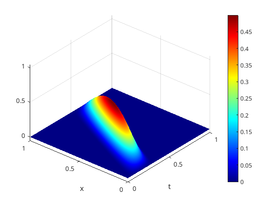
(a) $y_{d,1}$

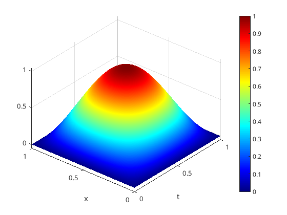
(b) $y_{d,2}$

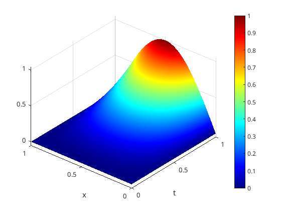
(c) $y_{d,3}$

Figure 3: Targets $y_{d,i}\in H_{0;0,}^{1,1}(Q)\cap H^{2}(Q)$, $i=1,2,3$.

(a) $y_{d,1}$

(b) $y_{d,2}$

(c) $y_{d,3}$

Figure 4: Convergence plots for the targets $y_{d,i}$, $i=1,2,3$, choosing $\varrho_{j}=2^{-j}$, $j=14,\ldots,23$ for the $L^{2}$-regularization where the reference solution $y_{\varrho_{j}}=y_{\varrho_{j}h}\in Y_{h}$ is computed via a finite element method on a uniform mesh with $n_{h}=131072$ simplicial elements and $m_{h}=65280$ DoFs with mesh size $h=2.7621$e$-3$.

(a) $y_{d,1}$

(b) $y_{d,2}$

(c) $y_{d,3}$

Figure 5: Convergence plots for the targets $y_{d,i}$, $i=1,2,3$, choosing $\varrho_{j}=10^{-j}$, $j=2,\ldots,11$ for the $L^{2}$-regularization where the reference solution $y_{\varrho_{j}}=y_{\varrho_{j}h}\in Y_{h}$ is computed via a finite element method on a uniform mesh with $n_{h}=131072$ simplicial elements and $m_{h}=65280$ DoFs with mesh size $h=2.7621$e$-3$.

In order to check the interpolation error estimates, we consider a sequence of fixed $\varrho_{j}>0$, $j\in\mathbb{N}$, and compute for each target $y_{d,i}$, $i=1,2,3$, a related state $y_{\varrho_{j}}=y_{\varrho_{j}h}\in Y_{h}$ on a fine mesh with $n_{h}=131072$ elements and $m_{h}=65280$ DoFs. In Figure 4 the results for $\varrho_{j}=2^{-j}$, $j=14,\ldots,23$ are depicted. We clearly see the predicted behavior, i.e., $|p_{\varrho}|_{H^{1}(Q)}\simeq\varrho^{3/4}$ and $|y_{d}-y_{\varrho}|_{H^{1}(Q)}\simeq\varrho^{1/4}$. Morover, we also plot the $L^{2}$-error of the state to the target, where we observe the behavior $\|y_{d}-y_{\varrho}\|_{L^{2}(Q)}\simeq\sqrt{\varrho}$, which fits perfectly to the theoretical findings. In Figure 5 we show the results for $\varrho_{j}=10^{-j}$, $j=2,\ldots,11$. Note, that after a while the $L^{2}$-convergence breaks down, as a result of the best approximation property of $Y_{h}$ in $L^{2}(Q)$ when computing $y_{\varrho_{j}}=y_{\varrho_{j}h}\in Y_{h}$. Having a closer look, this happens when $\varrho_{j}\simeq h^{4}$. This supports the optimal choice $\varrho=h^{4}$, since choosing a smaller parameter $\varrho>0$ will not lead to a better approximation of the desired target for a given mesh size $h>0$. Note, that the $H^{1}$-error seems to stagnate even earlier.

References

• [1] O. Axelsson and J. Karátson. Superior properties of the PRESB preconditioner for operators on two-by-two block form with square blocks. Numer. Math, 146(2):335–368, 2020.
• [2] O. Axelsson, M. Neytcheva, and A. Ström. An efficient preconditioning method for state box-constrained optimal control problems. J. Numer. Math., 26(4):185–207, 2018.
• [3] I. Babuška and M. Vogelius. Feedback and adaptive finite element solution of one-dimensional boundary value problems. Numer. Math., 44:75–102, 1984.
• [4] Z.-Z. Bai, M. Benzi, F. Chen, and Z.-Q. Wang. Preconditioned MHSS iteration methods for a class of block two-by-two linear systems with applications to distributed control problems. IMA J. Numer. Anal., 33(1):343–369, 2013.
• [5] Z.-Z. Bai and J.-Y. Pan. Matrix Analysis and Computations. SIAM, 2021.
• [6] M. Benzi, G. H. Golub, and J. Liesen. Numerical solution of saddle point problems. Acta Numer., 14:1–137, 2005.
• [7] J. Bey. Tetrahedral grid refinement. Computing, 55:355–378, 1995.
• [8] J. H. Bramble and J. E. Pasciak. A preconditioning technique for indefinite systems resulting from mixed approximations of elliptic problems. Math. Comp., 50(181):1–17, 1988.
• [9] M. Dauge. Elliptic Boundary Value Problems on Corner Domains, volume 1341 of Lecture Notes in Mathematics. Springer, Berlin, Heidelberg, 1988.
• [10] J. De los Reyes. Numerical PDE-Constrained Optimization. Springer Cham, 2015.
• [11] I. Dravins and M. Neytcheva. On the Numerical Solution of State- and Control-constrained Optimal Control Problems. Department of Information Technology, Uppsala Universitet, 2021.
• [12] H. C. Elman, D. J. Silvester, and A. J. Wathen. Finite elements and fast iterative solvers: With applications in incompressible fluid dynamics. Oxford University Press, 2005.
• [13] P. Gangl, R. Löscher, and O. Steinbach. Regularization and finite element error estimates for elliptic distributed optimal control problems with energy regularization and state or control constraints, 2023. arXiv:2306.15316.
• [14] P. Grisvard. Elliptic problems in nonsmooth domains, volume 69 of Classics in Applied Mathematics. SIAM, Philadelphia, 2011.
• [15] R. Herzog, M. Heinkenschloss, D. Kalise, G. Stadler, and E. Trélat, editors. Optimization and Control for Partial Differential Equations, volume 29 of Radon Series on Computational and Applied Mathematics. de Gruyter, 2022.
• [16] M. Hintermüller, K. Ito, and K. Kunisch. The primal-dual active set method as a semismooth Newton method. SIAM J. Optimization, 13:865–888, 2003.
• [17] M. Hinze, R. Pinnau, M. Ulbrich, and S. Ulbrich. Optimization with PDE Constraints, volume 23 of Mathematical Modelling: Theory and Applications. Springer-Verlag, Berlin, 2009.
• [18] M. Jung, U. Langer, A. Meyer, W. Queck, and M. Schneider. Multigrid preconditioners and their applications. In G. Telschow, editor, Third Multigrid Seminar, Biesenthal 1988, pages 11–52, Karl–Weierstrass–Institut Berlin, Report R–MATH–03/89, 1989.
• [19] K. Kunisch and S. Reiterer. A Gautschi time-stepping approach to optimal control of the wave equation. Appl. Numer. Math., 90:55–76, 2015.
• [20] O. A. Ladyzhenskaya. The boundary value problems of mathematical physics, volume 49 of Applied Mathematical Sciences. Springer, New York, 1985.
• [21] U. Langer, R. Löscher, O. Steinbach, and H. Yang. Mass-lumping discretization and solvers for distributed elliptic optimal control problems, 2023. arXiv:2304.14664.
• [22] U. Langer, R. Löscher, O. Steinbach, and H. Yang. An adaptive finite element method for distributed elliptic optimal control problems with variable energy regularization. Comput. Math. Appl., 160:1–14, 2024.
• [23] U. Langer, O. Steinbach, F. Tröltzsch, and H. Yang. Space-time finite element discretization of parabolic optimal control problems with energy regularization. SIAM J. Numer. Anal., 59(2):660–674, 2021.
• [24] U. Langer, O. Steinbach, F. Tröltzsch, and H. Yang. Unstructured space-time finite element methods for optimal control of parabolic equation. SIAM J. Sci. Comput., 43(2):A744–A771, 2021.
• [25] J. L. Lions. Contrôle optimal de systèmes gouvernés par des équations aux dérivées partielles. Dunod Gauthier-Villars, Paris, 1968.
• [26] R. Löscher and O. Steinbach. Space-time finite element methods for distributed optimal control of the wave equation. SIAM J. Numer. Anal., 62(1):452–475, 2024.
• [27] K.-A. Mardal and R. Winther. Preconditioning discretizations of systems of partial differential equations. Numer. Linear Algebra Appl., 18(1):1–40, 2011.
• [28] M. Neumüller and O. Steinbach. Regularization error estimates for distributed control problems in energy spaces. Math. Methods Appl. Sci., 44:4176–4191, 2021.
• [29] J. Pearson, M. Stoll, and A. Wathen. Preconditioners for state-constrained optimal control problems with moreau-yosida penalty function. Numer. Linear Algebra Appl., 21(1):81–97, 2014.
• [30] J. Pearson and A. Wathen. A new approximation of the Schur complement in preconditioners for PDE-constrained optimization. Numer. Linear Algebra Appl., 12(5):816–829, 2012.
• [31] G. Peralta and K. Kunisch. Mixed and hybrid Petrov–Galerkin finite element discretization for optimal control of the wave equation. Numer. Math., 150:591–627, 2022.
• [32] M. Rozložníík. Saddle-Point Problems and Their Iterative Solution. Nec̆as Center Series. Birkhäuser Cham, 2018.
• [33] J. W. Ruge and K. Stüben. Algebraic multigrid (AMG). In S. F. McCormick, editor, Multigrid Methods, pages 73–130. SIAM, Philadelphia, 1987.
• [34] A. Schiela and S. Ulbrich. Operator preconditioning for a class of inequality constrained optimal control problems. SIAM J. Optim., 24(1):435–466, 2014.
• [35] J. Schöberl and W. Zulehner. Symmetric indefinite preconditioners for saddle point problems with applications to PDE-constrained optimization problems. SIAM J. Matrix Anal. Appl., 29:752–773, 2007.
• [36] V. Schulz and G. Wittum. Transforming smoothers for pde constrained optimization problems. Comput. Visual. Sci., 11:207–219, 2008.
• [37] L. R. Scott and S. Zhang. Finite element interpolation of nonsmooth functions satisfying boundary conditions. Math. Comp., 54(190):483–493, 1990.
• [38] O. Steinbach and M. Zank. Coercive space-time finite element methods for initial boundary value problems. Electron. Trans. Numer. Anal., 52:154–194, 2020.
• [39] O. Steinbach and M. Zank. A generalized inf-sup stable variational formulation for the wave equation. J. Math. Anal. Appl., 505(1):Paper No. 125457, 24, 2022.
• [40] R. Stevenson. The completion of locally refined simplicial partitions created by bisection. Math. Comp., 77(261):227–241, 2008.
• [41] M. Stoll and A. Wathen. Preconditioning for partial differential equation constrained optimization with control constraints. Numer. Linear Algebra Appl., 19:53–71, 2012.
• [42] F. Tröltzsch. Optimal control of partial differential equations: Theory, methods and applications, volume 112 of Graduate Studies in Mathematics. American Mathematical Society, Providence, Rhode Island, 2010.
• [43] A. Wathen. Preconditioning. Acta Numerica, 24:329–376, 2015.
• [44] M. Zank. Inf-sup stable space-time methods for time-dependent partial differential equations, volume 38 of Computation in Engineering and Science. Verlag der Technischen Universität Graz, 2020.
• [45] W. Zulehner. Analysis of iterative methods for saddle point problems: a unified approach. Math. Comp., 71(238):479–505, 2002.