Dynamical heterogeneity and large deviations in the open quantum East glass model from tensor networks

Abstract

We study the non-equilibrium dynamics of the dissipative quantum East model via numerical tensor networks. We use matrix product states to represent evolution under quantum-jump unravellings for sizes beyond those accessible to exact diagonalisation. This allows us to demonstrate that dynamical heterogeneity accompanies slow relaxation, in analogy with what is seen in classical glassy systems. Furthermore, using variational matrix product operators we: (i) compute the spectral gap of the Lindbladian, and show that glassiness is enhanced in the presence of weak quantum fluctuations compared to the pure classical case, and (ii) obtain the dynamical large deviations by calculating the leading eigenvector of the tilted Lindbladian, and find clear evidence for a first-order active-inactive dynamical phase transition. We also show how to directly sample the rare quantum trajectories associated to the large deviations.

Introduction.- Kinetically constrained models (KCMs) serve as an important paradigm for understanding non-equilibrium dynamics. Originally introduced to model the steric interactions responsible for the slow relaxation of structural glasses [1, 2, 3, 4], classical KCMs provide the combination of simple static properties with complex cooperative dynamics due to constraints [5, 6, 7, 8, 9]. Quantum KCMs in turn appear in several contexts, one being Rydberg atoms where strong interactions are responsible for either “Rydberg blockade” (encoded in the PXP model [10, 11, 12]) or “facilitated” dynamics [13, 14, 15, 16, 17, 18, 19]; another, a scenario for non-ergodicity due to constraints rather than disorder [20, 21, 22, 23, 24, 25, 26, 27, 28, 29].

In this paper, we focus on the dynamics of quantum KCMs in the presence of an environment, specifically on the open quantum East model (OQEM) [30], which generalises the well-studied East model to a quantum dissipative setting. We consider both the typical dynamics and the large deviations of the OQEM using numerical tensor networks (TNs) [31, 32]. We simulate quantum trajectories of pure states under quantum-jump unravellings for large system sizes using matrix product states (MPS) [33, 34] as an ansatz for the wavefunction [35], an approach well suited to this problem, as constrained dynamics limits the growth of entanglement. We also use variational matrix product operators (vMPOs) [36] to directly approximate the eigenvectors of the Lindbladian and: (i) estimate the spectral gap of the generator of the dynamics in order to quantify the relaxation time, showing convincingly “re-entrant” behaviour [37], whereby a small amount of quantum fluctuations slows dynamics compared to the classical limit; (ii) calculate the dynamical large deviations (LDs) [38, 39, 40], showing the existence of an active-inactive dynamical phase transition, in analogy with the classical East model [41]. Our results extend the applicability of TN methods for the study of rare events in classical stochastic systems [42, 43, 44, 45, 46, 47, 48, 49, 50, 51, 52] to quantum stochastic systems.

Open Quantum East Model.- We consider an open quantum system whose evolution is given by a Lindblad–Gorini–Kossakowski–Sudarshan [53, 54] master equation, $\dot{\rho_{t}}=\mathcal{L}[\rho_{t}]$, where $\rho_{t}$ is the density matrix of the system at time $t$, with super-operator $\mathcal{L}$ that generates this dynamics (the so-called Lindbladian) [55],

$$\mathcal{L}[\bm{\cdot}]=-i[\hat{H},\bm{\cdot}]+\mathcal{D}[\bm{\cdot}].$$ (1)

The OQEM [30, 56] is defined in terms of a one-dimensional lattice of $N$ qubits with Hamiltonian

$$\hat{H}=\Omega\sum_{j=1}^{N}\hat{f}_{j}\hat{\sigma}_{j}^{x},$$ (2)

and dissipator

$$\mathcal{D}[\bm{\cdot}]=\sum_{\alpha=+,-}\sum_{j=1}^{N}\hat{J}_{\alpha,j}\bm{\cdot}\hat{J}_{\alpha,j}^{\dagger}-\frac{1}{2}\{\hat{J}_{\alpha,j}^{\dagger}\hat{J}_{\alpha,j},\bm{\cdot}\}$$ (3)

with jump operators

$$\hat{J}_{+,j}=\sqrt{\gamma}\hat{f}_{j}\hat{\sigma}^{+}_{j},\,\,\hat{J}_{-,j}=\sqrt{\kappa}\hat{f}_{j}\hat{\sigma}^{-}_{j},$$ (4)

where $\hat{\sigma}^{+}_{j}=\ket{1}\bra{0}$ and $\hat{\sigma}^{-}_{j}=\ket{0}\bra{1}$ are the spin-$1/2$ ladder operators acting on site $j$, with $\hat{\sigma}^{x}_{j}=\hat{\sigma}^{+}_{j}+\hat{\sigma}^{-}_{j}$.

Both the term of the Hamiltonian (2) and the jump operators (4) that act on site $j$ depend on the kinetic constraint operator $\hat{f}_{j}$ [30]. This is a projector that depends on the state of the neighbouring site $j-1$ and acts as an operator-valued rate that determines whether a local transition can take place depending on its neighbours, in analogy with how classical KCMs are defined [5]. The form of $\hat{f}_{j}$ is chosen [30] such that the stationary state of Eq. (1) is the same as in the unconstrained case (when all $\hat{f}_{j}=1$),

$$\rho^{\rm ss}=\bigotimes_{j=1}^{N}\left(p_{\rm e}\ket{e}\bra{e}_{j}+p_{\rm u}\ket{u}\bra{u}_{j}\right),$$ (5)

where $\ket{u}_{j},\ket{e}_{j}$ are the eigenstates of the local stationary density matrix at $j$, and $p_{\rm u},p_{\rm e}$ its eigenvalues [30], with $p_{\rm u}+p_{\rm e}=1$. We label the states according to their probabilities, such that $p_{\rm e}\leq p_{\rm u}$, and we call $\ket{e}_{j}$ excited and $\ket{u}_{j}$ local unexcited states. The constraint then reads [30]

$$\hat{f}_{j}=\ket{e}\bra{e}_{j-1}\equiv\hat{P}_{j-1}^{e},$$ (6)

where $\hat{P}_{j}^{e}$ is the projector onto the local excited state. The local states and transitions of the OQEM are illustrated in Fig. 1(a-c). As shown originally in Ref. [30], the choice Eq. (6) guarantees that the stationary state of the OQEM is the product state Eq. (5). In the limit $\Omega=0$ the dynamics generated by Eqs. (1-4) is equivalent to that of the classical East model at temperature $1/\ln{(\gamma/\kappa)}$ [cf. Fig. 1(c)], so that by tuning $\Omega$ we can investigate the interplay of classical and quantum relaxation mechanisms. For convenience, in what follows we study the OQEM with the open boundary condition $\hat{P}_{0}^{e}=1$.

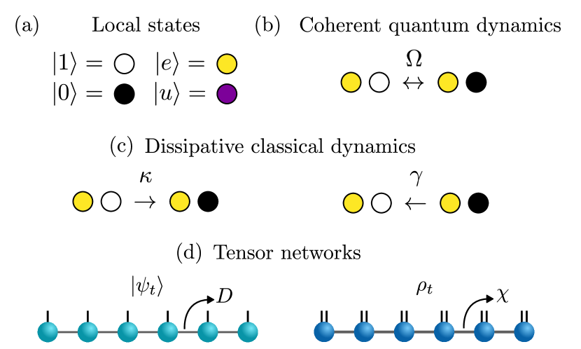
Figure 1: Open quantum East model and TNs. (a) Local classical (or computational) basis states $\ket{1}$ and $\ket{0}$ (“up” or “down”) are represented by empty (white) or filled (black) circles, respectively. The local “excited” and “unexcited” states, $\ket{\rm e}$ and $\ket{\rm u}$, are superpositions (see Refs. [30, 56] for their specific forms), shown as bright (yellow) and dark (purple) circles, respectively. (b) Coherent transitions are allowed only if the neighbour to the left has a projection onto the excited state, see Eq. (2). (c) Same for dissipative transitions, see Eq. (4). (d) MPS are used to approximate wavefunctions, $\ket{\psi_{t}}$, and MPOs density matrices, $\rho_{t}$. The internal bonds have dimensions $D$ and $\chi$, respectively. Open (physical) legs have dimensions $2$ and $2\times 2$, respectively.

Tensor networks.- TNs are efficient parametrisations of high dimensional objects, such as states and operators, in terms of smaller tensorial objects [33, 34, 57, 58, 59, 60, 61, 32]. An especially useful decomposition for the wavefunction of a one dimensional system is the matrix product state (MPS) [34], shown pictorially in Fig. 1(d): each lattice site is given its own rank-3 tensor (blue circles), with physical dimension $d$ ($=2$ in our case) for the vertical legs, and virtual or bond dimension $D$ for each of the horizontal legs. Each tensor is connected to its neighbouring tensors along the lattice sites via its virtual legs, with the many-body state obtained by contracting (i.e. multiplying and summing over the connected indices) all virtual legs. The number of parameters in such an MPS is $\mathcal{O}(NdD^{2})$, which is much smaller than what is required to represent a generic vector for large $N$, at the price of only accurately describing a subset of the Hilbert space with entanglement upper-bounded by $S_{E}\leq 2\log D$, which happens to approximate well ground states of local Hamiltonians [62].

A similar ansatz can be applied to operators acting on a 1D system. Such a matrix product operator (MPO) [63, 64, 65] is depicted in Fig. 1(d) for the density matrix: each local tensor is of rank-4, with two physical dimensions (each $d=2$) and two virtual dimensions (each $\chi$). For physical states, this MPO needs to be positive, and while, strictly speaking, positivity cannot even be decided at the level of the local tensors [66, 67], in practice many MPO algorithms can approximately preserve it .

We use both MPS and MPOs to investigate the OQEM for sizes beyond those accessible to exact diagonalisation: (i) MPS to simulate the quantum trajectories of pure states evolving under a quantum jump unravelling [69]; (ii) variational MPOs (vMPOs) to estimate the spectral gap of the Lindbladian, and to estimate the leading eigenvectors of tilted Lindbladians that encode the large deviations [70]; and (iii) both in conjunction to efficiently generate quantum trajectories that realise the dynamical large deviations. For details of the methods used see Ref. [71].

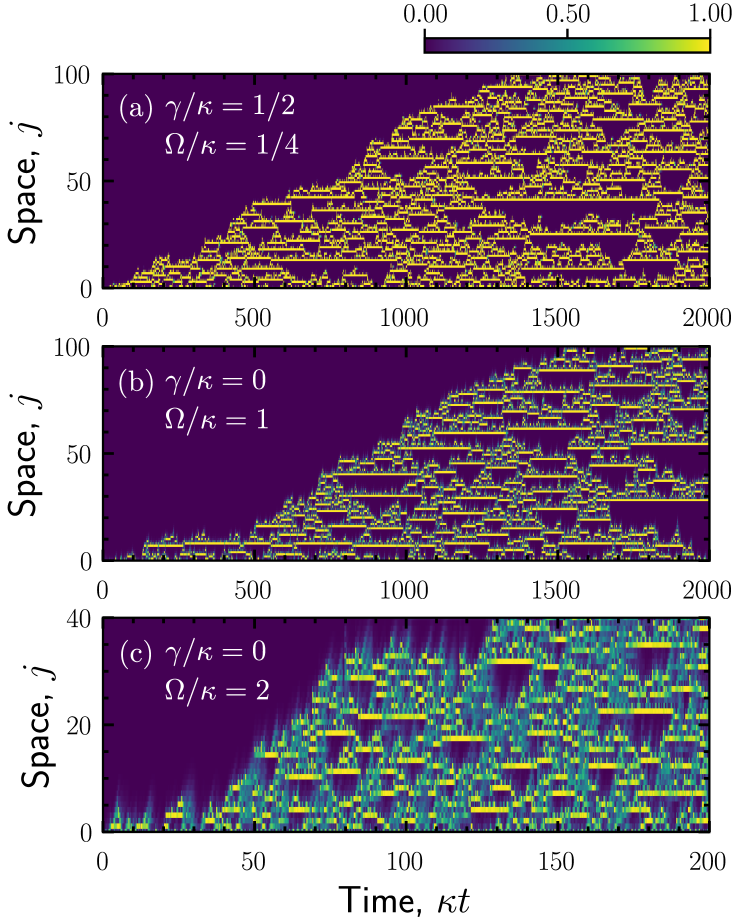
Figure 2: Quantum jump trajectories of the OQEM. (a) Local projection onto the excited, $\braket{\hat{P}_{j}^{e}}_{t}$, as a function of rescaled time, $\kappa t$, from a quantum trajectory starting from $\ket{\psi_{0}}=\otimes\bigotimes_{j=1}^{N}\ket{u}_{j}$ , for $\gamma/\kappa=1/2$, $\Omega/\kappa=1/4$. (Note that the open boundary conditions are such that site $j=1$ is always allowed to flip.) (b) Same for $\gamma=0$, $\Omega/\kappa=1$. (c) Same for $\gamma=0$, $\Omega/\kappa=2$ (note that both system size and overall time are smaller than in other panels).

Quantum trajectories and dynamical heterogeneity.- We study first the quantum trajectories of the OQEM under a quantum jump unravelling [72]. This corresponds to a continuous-time quantum Markov chain where the pure state $\ket{\psi_{t}}$ is evolved deterministically, $\ket{\psi_{t+\Delta t}}=e^{-i\Delta t\hat{H}_{\rm eff}}\ket{\psi_{t}}/||e^{-i\Delta t\hat{H}_{\rm eff}}\ket{\psi_{t}}||$ (with $\hat{H}_{\rm eff}=\hat{H}-\frac{i}{2}\sum_{\alpha,j}\hat{J}^{\dagger}_{\alpha,j}\hat{J}_{\alpha,j}$), punctuated stochastically by quantum jumps, $\ket{\psi_{t}}\to\ket{\psi^{\prime}_{t}}=\hat{J}_{\mu}\ket{\psi_{t}}/||\hat{J}_{\mu}\ket{\psi_{t}}||$, with transition rates $w_{\mu}(\ket{\psi_{t}})={\braket{\psi_{t}}{\hat{J}^{\dagger}_{\mu}\hat{J}_{\mu}}{\psi_{t}}}{\braket{\psi_{t}}{\psi_{t}}}$. By modelling the state using a MPS ansatz with a bond dimension that can be dynamically adjusted [69] to account for the fluctuating levels of entanglement, we can simulate these trajectories for sizes much larger than those accessible by exact methods in previous works [30, 56]. For implementation details see Ref. [71].

Figure 2 shows trajectories starting with all sites in the unexcited state, $\ket{\psi_{0}}=\bigotimes_{j=1}^{N}\ket{u}_{j}$, and we plot the local projections onto the excited state, $\braket{\hat{P}_{j}^{e}}_{t}=\braket{\psi_{t}}{\hat{P}_{j}^{e}}{\psi_{t}}$. Panel (a) shows a trajectory for $\gamma/\kappa=1/2$ and $\Omega/\kappa=1/4$ with system size $N=100$ and total time $\kappa T=2000$: despite the coherent driving, it being relatively weak means that quantum superpositions are mostly suppressed; the trajectory looks like those in the classical model, with the characteristic “space-time bubbles” of inactivity that give rise to dynamical heterogeneity [73]. Panel (b) shows a trajectory for $\gamma/\kappa=0$ (i.e. “zero temperature”) and $\Omega/\kappa=1$: the absence of the dissipative excitation process means that the coherent driving is the only mechanism to give rise to relaxation; the dynamical fluctuations here are greater than in the weakly perturbed classical case, and the system exhibits a large degree of dynamical heterogeneity that is quantum in origin. Panel (c) shows the same but for lager driving, $\Omega/\kappa=2$ (for $N=40$ and $T=100$ as relaxation is faster in this case): the quantum effects are more pronounced and the increased coherent driving reduces dynamical fluctuations.

Relaxation timescale and re-entrant glassy behaviour.- The quantum trajectories of Fig. 2 illustrate the basic physics of the OQEM. Due to the constraint, relaxation propagates from regions with excitations to regions without. For an empty initial condition such as that of Fig. 2 (with an active boundary), in the classical limit it is known that the excited region expands ballistically into the unexcited region, eventually relaxing the whole system (proven rigorously in the asymptotic limit in Ref. [74] for such KCMs). The finite space and time trajectories of Fig. 2 suggest that this is also the case for the OQEM. Relaxation speed is determined both by the dissipative excitation process, controlled by the “classical” rate $\gamma/\kappa$, and by the coherent process, of scaled strength $\Omega/\kappa$. As in the classical case [75, 41, 76, 77], the trajectories show coexistence of space-time regions of high and low activity. For small $\gamma/\kappa$ and $\Omega/\kappa$, relaxation is slow and glassy.

The typical relaxation timescale from an arbitrary configuration is given by the inverse of the spectral gap of the Lindbladian [79, 80, 81, 82]. We can estimate the gap using a variational optimisation of the eigenvectors of the Lindbladian represented as a MPO  [36] (see Ref. [71] for details). The results of this approach are shown in Fig. 3 where we plot the gap of the OQEM relative to the classical case,

$$g(\gamma/\kappa,\Omega/\kappa)=\frac{\delta(\gamma/\kappa,\Omega/\kappa)}{\delta(\gamma/\kappa,0)}-1,$$ (7)

as a function of the coherent driving $\Omega/\kappa$ for two values of the dissipative excitation rate, panel (a) showing $\gamma/\kappa=1/5$, and panel (b) $\gamma/\kappa=1/2$. The definition Eq. (7) makes $g>0$ if relaxation is faster than in the classical limit, and $g<0$ if it is slower. Figure 3 shows that the addition of a small amount of quantum coherence ($\Omega/\kappa\gtrsim 0$) enhances glassiness within the dynamics, a phenomenon sometimes referred to as quantum re-entrance [37]. When the strength of the quantum coherence is increased enough, the gap eventually increases resulting in a faster than classical relaxation. Our results seem to confirm the trend observed in Ref. [30] for a different KCM - the open quantum Fredrickson-Andersen model - for sizes up to $N=5$ (such that the Lindbladian can be diagonalised numerically exactly). In contrast, with our TN methods here we are able to reach up to sizes $N=36$ for the OQEM. Note that in Fig. 3 the relative gap Eq. (7) appears to converge with $N$, which suggests that the observed behaviour holds for larger $N$. Furthermore, the error bars for each data point are small (see Ref. [71] for details), indicating a reasonable approximation of eigenvalues of $\mathcal{L}$: while there is no guarantee that the TN method is approximating the eigenvalue with the smallest real part, at worst our results are an estimate of an upper bound to the spectral gap.

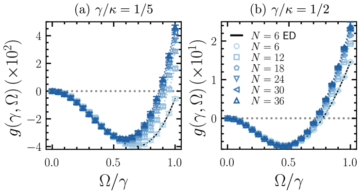
Figure 3: Re-entrant glassiness due to quantum fluctuations. (a) Relative gap $g(\gamma,\Omega)$ as a function of coherent driving relative to dissipative excitation rate, $\Omega/\gamma$, for $\gamma/\kappa=1/5$. The dotted line at zero separates the regime of faster-than-classical relaxation ($g>0$) from that of slower-than-classical ($g<0$). The symbols show the vMPO results for sizes $N=6-36$, and the dashed line shows the exact diagonalization result for $N=6$ for reference. (b) Same for $\gamma/\kappa=1/2$.

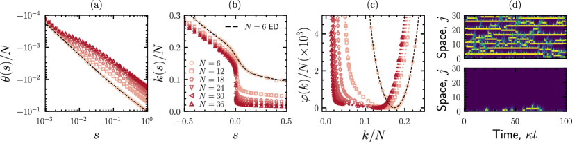
Figure 4: Dynamical large deviations and optimal sampling. (a) SCGF $\theta(s)/N$ as a function of $s$ from the vMPOs approximation to the leading eigenmatrix $L_{s}$. We show sizes $N=6-36$ (symbols) together with $N=6$ (dashed line) from exact diagonalisation for comparison. At small $s$, the SCGF goes as $\theta(s)\approx-sk(0)$ (dashed line), where $k(0)$ is the average dynamical activity at stationarity per unit time. For larger $s$ it departs from the linear response behaviour, with the crossover taking place at smaller $s$ with increasing size, indicative of a phase transition. (b) Dynamical activity, $k(s)/N=-\theta^{\prime}(s)/N$. The sharp drop (which gets more pronounced with size) indicates a first-order transition. (c) Rate function $\varphi(k)/N$. The broadening corresponds to (active/inactive) phase coexistence, which gets sharper with increasing size. (d) Characteristic quantum trajectories of the active ($s=-0.1$, top panel) and inactive ($s=0.1$, bottom panel) phases sampled using the optimal (Doob) dynamics.

Large deviations and dynamical phase transitions.- The pronounced fluctuations in the quantum trajectories of the OQEM shown in Fig. 2 are suggestive of coexistence between dynamics that is active and fast relaxing and dynamics that is inactive and unable to relax. Classically [75, 41] this behaviour is most naturally quantified through the statistics of the dynamical activity [83, 39, 84]. The equivalent for open quantum systems [70] is through the statistics of the total number of quantum jumps.

The probability to observe a number $K$ of quantum jumps in a quantum trajectory of time extent $t$ is $P_{t}(K)$. For large $t$ this probability will obey a large deviation (LD) principle [38], $P_{t}(K)\asymp e^{-t\varphi(K/t)}$, with $\varphi(k)$ the LD rate function . The same statistics is encoded in the moment generating function $Z_{t}(s)=\sum_{K}P_{t}(K)e^{-sK}$, where $s$ is the counting field conjugate to $K$ [70]. The corresponding LD principle reads $Z_{t}(s)\asymp e^{t\theta(s)}$, where $\theta(s)$ is the scaled cumulant generating function (SCGF) [70]. For open quantum dynamics, the SCGF can be obtained from the tilted Lindbladian $\mathcal{L}_{s}[\bm{\cdot}]=-i[\hat{H},\bm{\cdot}]+\mathcal{D}_{s}[\bm{\cdot}]$ [70], which for the OQEM has dissipator, cf. (3),

$$\mathcal{D}_{s}[\bm{\cdot}]=\sum_{\alpha=+,-}\sum_{j=1}^{N}e^{-s}\hat{J}_{\alpha,j}\bm{\cdot}\hat{J}_{\alpha,j}^{\dagger}-\frac{1}{2}\{\hat{J}_{\alpha,j}^{\dagger}\hat{J}_{\alpha,j},\bm{\cdot}\}.$$ (8)

Specifically, the SCGF $\theta(s)$ is the largest eigenvalue of $\mathcal{L}_{s}$, with right and left eigenmatrices, $\mathcal{L}_{s}[R_{s}]=\theta(s)R_{s}$ and $\mathcal{L}^{\dagger}_{s}[L_{s}]=\theta(s)L_{s}$ [70]. Knowing $\theta(s)$ we can recover the rate function, and thus the distribution of $K$, by inverting the Legendre transform, $\theta(s)=-\min_{k}[ks+\varphi(k)]$ [38].

We can compute the SCGF numerically for the OQEM by estimating either of the eigenmatrices $R_{s}$ or $L_{s}$ using non-Hermitian vMPOs [36]. In practice, we find the method is more stable and has a better accuracy when targeting $L_{s}$. The results for the SCGF obtained in this way are shown in Fig. 4 for the case of $\gamma/\kappa=0$ and $\Omega/\kappa=1$. For these parameters, we are able to find results with our desired accuracy of $\varepsilon\leq 10^{-3}$ for system sizes up to $N=36$ (see Ref. [71] for details). The SCGF $\theta(s)/N$ is shown in Fig. 4(a) as a function of $s$: for small $s\gtrsim 0$, the SCGF follows the (linear response) branch $\theta(s)\approx-sk(0)$ where $k(0)$ is the average $K$ (per unit time) in the stationary state (5) (black dashed line), while at $s_{c}(N)\gtrsim 0$ (which decreases with system size) there is a sharp crossover away from linear response. The tilted dynamical activity is given by the derivative of the SCGF, $k(s)=-\theta^{\prime}(s)$, and is shown in Fig. 4(b): this shows that the change at $s_{c}(N)\gtrsim 0$ in the SCGF corresponds to a sharp drop in activity, indicating a first-order dynamical phase transition in the large size limit. Figure 4(c) shows the corresponding rate function: the first-order transition manifests as large fluctuations in $K$ due to the coexistence between an active (large $K$) dynamical phase and and inactive (small $K$) one.

Optimal dynamics for sampling the large deviations.- Our MPO approximation to the left eigenmatrix of ${\mathcal{L}}_{s}$ allows us to realise the optimal dynamics that samples the rare quantum trajectories that realise the large deviations as controlled by $s$. This is done via the quantum generalisation [70, 86, 87, 88] of the classical generalised Doob transform [89, 90, 91, 92].

For quantum open systems it is important to note that the Lindbladian is not the quantum equivalent of a classical Markov generator, as it only generates the dynamics of the average state. The equivalent operator is what in Refs. [87, 88] is called “unravelled generator”, which generates the stochastic quantum trajectories. While one can do a “quantum Doob transform” [70, 86] at the level of the Lindbladian and obtain average behaviour compatible with $s\neq 0$, in order to generate actual rare tajectories at $s\neq 0$ optimally we need to perform a Doob transform at the level of the unravelled generator [87, 88]. This gives a stochastic jump dynamics with the same Hamiltonian, Eq. (2), but jumps executed by operators similar in form to those in Eq. (4) but with modified rates [88]

$$w^{s}_{\mu}(\ket{\psi_{t}})=e^{-s}\frac{\braket{\psi_{t}}{\hat{J}^{\dagger}_{\mu}L_{s}\hat{J}_{\mu}}{\psi_{t}}}{\braket{\psi_{t}}{L_{s}}{\psi_{t}}},$$ (9)

where $\mu$ stands for $\alpha=\pm 1,j$ for the OQEM, cf. Eq. (4). The MPO approximation of $L_{s}$ allows us to efficiently obtain Eq. (9) as a TN calculation (see Ref. [71] for details) in a way that generalises to quantum stochastic dynamics the TN approach of Refs. [48, 52].

We show quantum trajectories sampled optimally (i.e. on demand at the required value of $s$, without the need for post-processing) using our implementation of the optimal Doob dynamics in Fig. 4(d) for $N=30$. The top panel is for the active phase ($s=-0.1$) and shows a characteristic trajectory of high activity (without inactive space-time bubbles, cf. Fig. 2). The bottom panel is for the inactive phase ($s=0.1$) and shows a characteristic trajectory with activity only localised near the boundary.

Discussion.- By means of numerical tensor networks, we have investigated the non-equilibrium dynamics of the dissipative quantum East model. We have shown the existence of dynamical heterogeneities in the quantum trajectories, using an MPS approximation to the stochastic pure states. By estimating the spectral gap of the Lindbladian, we were able to show explicitly that the presence of weak quantum fluctuations increases the relaxation time for the model, thus enhancing glassiness and giving rise to re-entrance, i.e., non-monotonic behaviour of the relaxation time as a function of coherent driving. Finally, we investigated the large deviation statistics of the number of quantum jumps, showing that the model exhibits an active-inactive first-order phase transition, very similar to what occurs in classical KCMs. We demonstrated that the features above occur also when the only source of relaxation is through coherent processes (i.e., when the classical processes are at zero temperature). Furthermore, we showed how to efficiently sample trajectories corresponding to the dynamical large deviations by constructing an accurate approximation to the optimal Doob dynamics. Our results here are another step in expanding the range of tensor network methods to study stochastic dynamics and rare events [45, 46, 47, 48, 49, 50, 51, 52].

Acknowledgements.- We acknowledge financial support from EPSRC Grant no. EP/V031201/1. M.C.B. acknowledges support from Deutsche Forschungsgemeinschaft (DFG, German Research Foundation) under Germany’s Excellence Strategy – EXC-2111 – 390814868 and 499180199 (via FOR5522). L.C. was supported through an EPSRC Doctoral Award Prize. We acknowledge access to the University of Nottingham Augusta HPC service.

References

- Fredrickson and Andersen [1984] G. H. Fredrickson and H. C. Andersen, Phys. Rev. Lett. 53, 1244 (1984).
- Palmer et al. [1984] R. G. Palmer, D. L. Stein, E. Abrahams, and P. W. Anderson, Phys. Rev. Lett. 53, 958 (1984).
- Jäckle and Eisinger [1991] J. Jäckle and S. Eisinger, Z. Phys. B Condens. Matter 84, 115 (1991).
- Kob and Andersen [1993] W. Kob and H. C. Andersen, Phys. Rev. E 48, 4364 (1993).
- Ritort and Sollich [2003] F. Ritort and P. Sollich, Adv. Phys. 52, 219 (2003).
- Chandler and Garrahan [2010] D. Chandler and J. P. Garrahan, Annu. Rev. Phys. Chem. 61, 191 (2010).
- Garrahan et al. [2011] J. P. Garrahan, P. Sollich, and C. Toninelli, in Dynamical Heterogeneities in Glasses, Colloids, and Granular Media, International Series of Monographs on Physics, edited by L. Berthier, G. Biroli, J.-P. Bouchaud, L. Cipelletti, and W. van Saarloos (Oxford University Press, Oxford, UK, 2011) Chap. 10, pp. 341–366.
- Speck [2019] T. Speck, J. Stat. Mech.: Theory Exp. 2019 (8), 084015.
- Hasyim and Mandadapu [2023] M. R. Hasyim and K. K. Mandadapu, arXiv:2310.06584 (2023).
- Fendley et al. [2004] P. Fendley, K. Sengupta, and S. Sachdev, Phys. Rev. B 69, 075106 (2004).
- Lesanovsky [2011] I. Lesanovsky, Phys. Rev. Lett. 106, 025301 (2011).
- Turner et al. [2018] C. J. Turner, A. A. Michailidis, D. A. Abanin, M. Serbyn, and Z. Papić, Nat. Phys. 14, 745 (2018).
- Ates et al. [2007] C. Ates, T. Pohl, T. Pattard, and J. M. Rost, Phys. Rev. Lett. 98, 023002 (2007).
- Amthor et al. [2010] T. Amthor, C. Giese, C. S. Hofmann, and M. Weidemüller, Phys. Rev. Lett. 104, 013001 (2010).
- Lesanovsky and Garrahan [2014] I. Lesanovsky and J. P. Garrahan, Phys. Rev. A 90, 011603 (2014).
- Hoening et al. [2014] M. Hoening, W. Abdussalam, M. Fleischhauer, and T. Pohl, Phys. Rev. A 90, 021603 (2014).
- Valado et al. [2016] M. M. Valado, C. Simonelli, M. D. Hoogerland, I. Lesanovsky, J. P. Garrahan, E. Arimondo, D. Ciampini, and O. Morsch, Phys. Rev. A 93, 040701 (2016).
- Ostmann et al. [2019] M. Ostmann, M. Marcuzzi, J. P. Garrahan, and I. Lesanovsky, Phys. Rev. A 99, 060101 (2019).
- Causer et al. [2020] L. Causer, I. Lesanovsky, M. C. Bañuls, and J. P. Garrahan, Phys. Rev. E 102, 052132 (2020).
- van Horssen et al. [2015] M. van Horssen, E. Levi, and J. P. Garrahan, Phys. Rev. B 92, 100305 (2015).
- Lan et al. [2018] Z. Lan, M. van Horssen, S. Powell, and J. P. Garrahan, Phys. Rev. Lett. 121, 040603 (2018).
- Pancotti et al. [2020] N. Pancotti, G. Giudice, J. I. Cirac, J. P. Garrahan, and M. C. Bañuls, Phys. Rev. X 10, 021051 (2020).
- Deger et al. [2022a] A. Deger, S. Roy, and A. Lazarides, Phys. Rev. Lett. 129, 160601 (2022a).
- Deger et al. [2022b] A. Deger, A. Lazarides, and S. Roy, Phys. Rev. Lett. 129, 190601 (2022b).
- Valencia-Tortora et al. [2022] R. J. Valencia-Tortora, N. Pancotti, and J. Marino, PRX Quantum 3, 020346 (2022).
- Carollo et al. [2022] F. Carollo, M. Gnann, G. Perfetto, and I. Lesanovsky, Phys. Rev. B 106, 094315 (2022).
- Zadnik et al. [2021] L. Zadnik, K. Bidzhiev, and M. Fagotti, SciPost Phys. 10, 099 (2021).
- Bertini et al. [2023a] B. Bertini, P. Kos, and T. Prosen, Localised dynamics in the floquet quantum east model (2023a), arXiv:2306.12467 .
- Bertini et al. [2023b] B. Bertini, C. D. Fazio, J. P. Garrahan, and K. Klobas, Exact quench dynamics of the floquet quantum east model at the deterministic point (2023b), arXiv:2310.06128 .
- Olmos et al. [2012] B. Olmos, I. Lesanovsky, and J. P. Garrahan, Phys. Rev. Lett. 109, 020403 (2012).
- Orús [2019] R. Orús, Nat. Revs. Phys. 1, 538 (2019).
- Bañuls [2023] M. C. Bañuls, Annu. Rev. Condens. Matter Phys. 14, 173 (2023).
- Verstraete et al. [2008] F. Verstraete, V. Murg, and J. Cirac, Adv. Phys 57, 143 (2008).
- Schollwöck [2011] U. Schollwöck, Ann. Phys. 326, 96 (2011), january 2011 Special Issue.
- Daley [2014] A. J. Daley, Adv. Phys. 63, 77 (2014).
- Cui et al. [2015] J. Cui, J. I. Cirac, and M. C. Bañuls, Phys. Rev. Lett. 114, 220601 (2015).
- Markland et al. [2011] T. E. Markland, J. A. Morrone, B. J. Berne, K. Miyazaki, E. Rabani, and D. R. Reichman, Nat. Phys. 7, 134 (2011).
- Touchette [2009] H. Touchette, Phys. Rep. 478, 1 (2009).
- Garrahan [2018] J. P. Garrahan, Physica A: Stat. Mech. Appl. 504, 130 (2018), lecture Notes of the 14th International Summer School on Fundamental Problems in Statistical Physics.
- Jack [2020] R. L. Jack, Eur. Phys. J. B 93, 74 (2020).
- Garrahan et al. [2007] J. P. Garrahan, R. L. Jack, V. Lecomte, E. Pitard, K. van Duijvendijk, and F. van Wijland, Phys. Rev. Lett. 98, 195702 (2007).
- Gorissen et al. [2009] M. Gorissen, J. Hooyberghs, and C. Vanderzande, Phys. Rev. E 79, 020101 (2009).
- Gorissen and Vanderzande [2012] M. Gorissen and C. Vanderzande, Phys. Rev. E 86, 051114 (2012).
- Gorissen et al. [2012] M. Gorissen, A. Lazarescu, K. Mallick, and C. Vanderzande, Phys. Rev. Lett. 109, 170601 (2012).
- Bañuls and Garrahan [2019] M. C. Bañuls and J. P. Garrahan, Phys. Rev. Lett. 123, 200601 (2019).
- Helms et al. [2019] P. Helms, U. Ray, and G. K.-L. Chan, Phys. Rev. E 100, 022101 (2019).
- Helms and Chan [2020] P. Helms and G. K.-L. Chan, Phys. Rev. Lett. 125, 140601 (2020).
- Causer et al. [2021] L. Causer, M. C. Bañuls, and J. P. Garrahan, Phys. Rev. E 103, 062144 (2021).
- Causer et al. [2022] L. Causer, M. C. Bañuls, and J. P. Garrahan, Phys. Rev. Lett. 128, 090605 (2022).
- Gu and Zhang [2022] J. Gu and F. Zhang, New J. Phys. 24, 113022 (2022).
- Strand et al. [2022] N. E. Strand, H. Vroylandt, and T. R. Gingrich, J. Chem. Phys 156, 221103 (2022).
- Causer et al. [2023] L. Causer, M. C. Bañuls, and J. P. Garrahan, Phys. Rev. Lett. 130, 147401 (2023).
- Lindblad [1976] G. Lindblad, Commun. Math. Phys. 48, 119 (1976).
- Gorini et al. [1976] V. Gorini, A. Kossakowski, and E. C. G. Sudarshan, J. Math. Phys. 17, 821 (1976).
- Gardiner and Zoller [2004] C. Gardiner and P. Zoller, Quantum noise (Springer, 2004).
- Rose et al. [2022] D. C. Rose, K. Macieszczak, I. Lesanovsky, and J. P. Garrahan, Phys. Rev. E 105, 044121 (2022).
- Orús [2014] R. Orús, Ann. Phys. 349, 117 (2014), arXiv:1306.2164 .
- Bridgeman and Chubb [2017] J. C. Bridgeman and C. T. Chubb, J. Phys. A: Math. Theor. 50, 223001 (2017).
- Silvi et al. [2019] P. Silvi, F. Tschirsich, M. Gerster, J. Jünemann, D. Jaschke, M. Rizzi, and S. Montangero, SciPost Phys. Lect. Notes , 8 (2019).
- Ran et al. [2020] S.-J. Ran, E. Tirrito, C. Peng, X. Chen, L. Tagliacozzo, G. Su, and M. Lewenstein, Tensor Network Contractions, Lecture Notes in Physics (Springer International Publishing, 2020).
- Okunishi et al. [2022] K. Okunishi, T. Nishino, and H. Ueda, J. Phys. Soc. Jpn 91, 062001 (2022).
- Cirac et al. [2021] J. I. Cirac, D. Pérez-García, N. Schuch, and F. Verstraete, Rev. Mod. Phys. 93, 045003 (2021).
- Verstraete et al. [2004] F. Verstraete, J. J. García-Ripoll, and J. I. Cirac, Phys. Rev. Lett. 93, 207204 (2004).
- Zwolak and Vidal [2004] M. Zwolak and G. Vidal, Phys. Rev. Lett. 93, 207205 (2004).
- Pirvu et al. [2010] B. Pirvu, V. Murg, J. I. Cirac, and F. Verstraete, New J. Phys. 12, 025012 (2010).
- Kliesch et al. [2014] M. Kliesch, D. Gross, and J. Eisert, Phys. Rev. Lett. 113, 160503 (2014).
- De las Cuevas et al. [2016] G. De las Cuevas, T. S. Cubitt, J. I. Cirac, M. M. Wolf, and D. Pérez-García, J. Math. Phys. 57, 071902 (2016).
- Note [1] An ansatz worth mentioning is the purification ansatz [63, 103, 66].While this preserves positivity, it is computationally more expensive and more restricted.
- Finsterhölzl et al. [2020] R. Finsterhölzl, M. Katzer, A. Knorr, and A. Carmele, Entropy 22, 10.3390/e22090984 (2020).
- Garrahan and Lesanovsky [2010] J. P. Garrahan and I. Lesanovsky, Phys. Rev. Lett. 104, 160601 (2010).
- [71] See Supplemental Material at [URL] for more details, which includes Refs. [93-104].
- Plenio and Knight [1998] M. B. Plenio and P. L. Knight, Rev. Mod. Phys. 70, 101 (1998).
- Garrahan and Chandler [2002] J. P. Garrahan and D. Chandler, Phys. Rev. Lett. 89, 035704 (2002).
- Blondel [2013] O. Blondel, Stoch. Process. Their Appl. 123, 3430 (2013).
- Merolle et al. [2005] M. Merolle, J. P. Garrahan, and D. Chandler, Proc. Natl. Acad. Sci. USA 102, 10837 (2005).
- Katira et al. [2016] S. Katira, K. K. Mandadapu, S. Vaikuntanathan, B. Smit, and D. Chandler, Elife 5, e13150 (2016).
- Klobas et al. [2023] K. Klobas, C. D. Fazio, and J. P. Garrahan, Exact ”hydrophobicity” in deterministic circuits: dynamical fluctuations in the floquet-east model (2023), arXiv:2305.07423 .
- Note [2] This is different from the timescale to relax from the most unfavourable initial state, as in Fig. 2, whose timescale is related to the “cutoff phenomenon” [104] of Markov chains.
- Cai and Barthel [2013] Z. Cai and T. Barthel, Phys. Rev. Lett. 111, 150403 (2013).
- Znidaric [2015] M. Znidaric, Phys. Rev. E 92, 042143 (2015).
- Macieszczak et al. [2016] K. Macieszczak, M. Guta, I. Lesanovsky, and J. P. Garrahan, Phys. Rev. Lett. 116, 240404 (2016).
- Zhou et al. [2022] B. Zhou, X. Wang, and S. Chen, Phys. Rev. B 106, 064203 (2022).
- Lecomte and Tailleur [2007] V. Lecomte and J. Tailleur, J. Stat. Mech. 2007, P03004 (2007).
- Maes [2020] C. Maes, Phys. Rep. 850, 1 (2020).
- Note [3] For the OQEM this is guaranteed as is gapped and its stationary state is unique.
- Carollo et al. [2018] F. Carollo, J. P. Garrahan, I. Lesanovsky, and C. Pérez-Espigares, Phys. Rev. A 98, 010103 (2018).
- Carollo et al. [2019] F. Carollo, R. L. Jack, and J. P. Garrahan, Phys. Rev. Lett. 122, 130605 (2019).
- Carollo et al. [2021] F. Carollo, J. P. Garrahan, and R. L. Jack, J. Stat. Phys. 184, 13 (2021).
- Borkar et al. [2003] V. S. Borkar, S. Juneja, and A. A. Kherani, Commun. Inf. Syst. 3, 259 (2003).
- Jack and Sollich [2010] R. L. Jack and P. Sollich, Prog. Theor. Phys. Supp. 184, 304 (2010).
- Chetrite and Touchette [2015] R. Chetrite and H. Touchette, Ann. Henri Poincaré 16, 2005 (2015).
- Garrahan [2016] J. P. Garrahan, J. Stat. Mech.: Theory Exp 2016, 073208 (2016).
- Hastings [2007] M. B. Hastings, J. Stat. Mech.: Theory Exp 2007, P08024 (2007).
- Verstraete and Cirac [2006] F. Verstraete and J. I. Cirac, Phys. Rev. B 73, 094423 (2006).
- Eisert et al. [2010] J. Eisert, M. Cramer, and M. B. Plenio, Rev. Mod. Phys. 82, 277 (2010).
- Maki et al. [2023] J. A. Maki, A. Berti, I. Carusotto, and A. Biella, SciPost Phys. 15, 152 (2023).
- Trotter [1959] H. F. Trotter, Proc. American Math. Soc. 10, 545 (1959).
- Vovk and Pichler [2022] T. Vovk and H. Pichler, Phys. Rev. Lett. 128, 243601 (2022).
- Mascarenhas et al. [2015] E. Mascarenhas, H. Flayac, and V. Savona, Phys. Rev. A 92, 022116 (2015).
- Chan and Van Voorhis [2005] G. K.-L. Chan and T. Van Voorhis, J. Chem. Phys. 122, 204101 (2005).
- Zhang et al. [2020] D.-W. Zhang, Y.-L. Chen, G.-Q. Zhang, L.-J. Lang, Z. Li, and S.-L. Zhu, Phys. Rev. B 101, 235150 (2020).
- Guo et al. [2022] Z. Guo, Z.-T. Xu, M. Li, L. You, and S. Yang, Variational Matrix Product State Approach for Non-Hermitian System Based on a Companion Hermitian Hamiltonian (2022), arXiv:2210.14858 .
- de las Cuevas et al. [2013] G. de las Cuevas, N. Schuch, D. Pérez-García, and J. I. Cirac, New J. Phys. 15, 123021 (2013).
- Aldous and Diaconis [1986] D. Aldous and P. Diaconis, Am. Math. Mon. 93, 333 (1986).