Randomized Greedy Methods for Weak Submodular Sensor Selection with Robustness Considerations

Abstract

We study a pair of budget- and performance-constrained weak submodular maximization problems. For computational efficiency, we explore the use of stochastic greedy algorithms which limit the search space via random sampling instead of the standard greedy procedure which explores the entire feasible search space. We propose a pair of stochastic greedy algorithms, namely, Modified Randomized Greedy (MRG) and Dual Randomized Greedy (DRG) to approximately solve the budget- and performance-constrained problems, respectively. For both algorithms, we derive approximation guarantees that hold with high probability. We then examine the use of DRG in robust optimization problems wherein the objective is to maximize the worst-case of a number of weak submodular objectives and propose the Randomized Weak Submodular Saturation Algorithm (Random-WSSA). We further derive a high-probability guarantee for when Random-WSSA successfully constructs a robust solution. Finally, we showcase the effectiveness of these algorithms in a variety of relevant uses within the context of Earth-observing LEO constellations which estimate atmospheric weather conditions and provide Earth coverage.

Keywords: Aerospace; decision making and autonomy, sensor data fusion; distributed optimization for large-scale systems; large scale optimization problems; modelling and decision making in complex systems; probabilistic robustness; robustness analysis.

1 Introduction

In sensor selection problems, especially those involving an extensive network of sensors, one often needs to select an optimal subset for a given task rather than using all available due to restrictions on resources. Such restrictions, usually modeled in terms of constraints on the cardinality or the cost of the feasible solutions, introduce the need to design principled decision-making algorithms for the creation of task-optimal selections of sensors that deliver high performance while adhering to the inherent resource, performance and robustness constraints. These problems occur naturally in many areas such as power system monitoring [1, 2], economics and algorithmic game theory [3, 4, 5], and finance [6]. In this work, we motivate the problem setting by considering low-Earth orbit (LEO) constellations of Earth-observing satellites [7].

The problem of choosing the optimal set of sensors is a computationally challenging combinatorial optimization that is known to be NP-hard [8]. Because of this complexity and theoretical barrier, a considerable amount of research has delved into creating heuristic algorithms aimed at providing approximate solutions for the problem.

Particularly well-known is the scenario where the objective can be formulated using a function that is both monotone nondecreasing and submodular, i.e., a set function that has the familiar property of demonstrating diminishing marginal gains. When the sensor selection is made in the presence of a cardinality constraint on the number of sensors, a proven result is that the so-called Greedy algorithm achieves an approximation factor of $(1-1/e)$ in comparison to the optimal solution [9]. Specifically, at each iteration, the Greedy algorithm considers each element in the set of remaining sensors, evaluates them in terms of marginal gain, and adds the element with the highest marginal gain to the set of selected elements.

Modified versions of the conventional greedy algorithm have been developed for addressing sensor selection problems with the more general case of budget constraints [10]. In this case, each sensor incurs a cost, and the decision-maker is restricted by a predetermined budget for their selections. The dual of this problem, where the objective is to identify the most cost-effective set of sensors to meet a specific performance constraint, has also been considered [11].

In situations involving a large number of sensors, the computational demands of Greedy become impractical due to the necessity of evaluating the marginal gain of every remaining sensor at each iteration. In [12], a computationally cheaper alternative is proposed, often referred to as the Stochastic or Randomized Greedy algorithm in the literature. This approach limits the function evaluations to a randomly sampled subset of the remaining sensors during each iteration and enjoys theoretical assurances concerning the expected performance of the constructed solution relative to the optimal solution. Expanding upon this randomized algorithm, [13] accounts for situations where the performance objective is defined by a weak submodular function, which is a function that is either submodular or closely approximates submodularity. Moreover, the authors derive a theoretical guarantee that holds with high probability for the performance of the randomized greedy algorithm in the weak submodular regime. However, it is important to note that the setting they consider is restricted solely to the cardinality-constrained case and does not take into account the highly nontrivial generalization of this setting to one involving the presence of a budget constraint and nonuniform selection costs.

In this work, we draw inspiration from the previously aforementioned work to propose a pair of novel extensions to the Randomized Greedy algorithm for use in budget- and performance-constrained problems, namely, the Modified Randomized Greedy (MRG) and Dual Randomized Greedy (DRG) algorithms, respectively. For both cases, we assume that the performance objective is characterized by a weak submodular function and that the sensor costs are simply additive. To the best of our knowledge, the use of randomized greedy algorithms in these two scenarios is a novel approach. In the ensuing discussion, we further derive theoretical guarantees that hold with high probability on the approximation factors for both algorithms. As expected, in the case where the performance objectives are not weak submodular but rather submodular, and where the standard greedy procedure is used instead of randomized greedy, both of the derived theoretical guarantees reduce to the standard results proven in the literature.

We further examine the use of the proposed DRG algorithm in the context of robust multi-objective submodular maximization where the robustness is captured by maximizing the worst objective as opposed to the maximization of the average of all objective functions. This notion of worst-case robustness extends the setting explored in [14] which proposes the Submodular Saturation Algorithm (SSA) in the presence of multiple objective functions which are all monotone nondecreasing and submodular. We propose a modified version of the algorithm, which we name Randomized Weak Submodular Saturation Algorithm (Random-WSSA), and likewise derive a theoretical guarantee on the performance of the algorithm that holds with high probability.

A preliminary version of this paper was presented in [15]. This paper represents a substantial expansion to its preliminary version. It incorporates extensive additional content, comprising more in-depth discussions and a broader set of experimental findings. Crucially, this paper introduces entirely new elements, encompassing novel theoretical insights, new algorithms, and experimental investigations regarding the setting of multi-objective worst-case robustness.

The remainder of the paper is organized as follows: In Section (2), we motivate our work in the context of LEO satellite constellations while in Section (3) we furnish the required preliminary information used in the rest of the work In Section (4), we introduce the MRG and the DRG algorithms and derive the theoretical bounds on their approximation ratios. In Section (5), we introduce Random-WSSA for the multi-objective robustness considerations and derive the theoretical guarantees on its success. Finally, in Section (6), we corroborate our theoretical results by providing numerical examples demonstrating the efficacy of the three proposed algorithms for sensor selection in Earth-observation tasks, as well as in multi-objective robustness scenarios.

2 Motivation: Satellite Sensing Networks

We start by presenting an illustrative motivating example within the field of LEO satellite constellations. Over the past few years, there has been a growing interest in satellite mission designs to use a cluster of simpler satellites rather than relying on a single intricate satellite. This trend has made the use of CubeSat-based designs [16] more commonplace, such as the constellation depicted in Figure (1). Constellations built on such concepts provide mission designers with various advantages. These advantages include cost savings in the design and launch expenses [17], increased redundancy to address potential failures, and improved temporal resolution in observations due to more frequent revisits [18]. Some examples of missions that have achieved success with this design philosophy are the NASA TROPICS mission [19] and the Planet Labs Flock Constellation [20]. The NASA TROPICS mission had as its primary objective to acquire temporally dense observations of weather phenomena, while the objective of the Flock Constellation was high-resolution imaging of the Earth’s surface. Proposed uses for CubeSat-based missions include many types of Earth science-related applications [21, 16], as well as disaster management, natural hazard response [22, 23] and air traffic monitoring [24, 25].

Naturally, as the number of such LEO constellations, as well as the number of satellites in the constellation increases, more human operators are needed for their supervision and operation. As previously discussed, one frequent mode of operation may involve the selection of only a subset of the satellites to use for sensing at each time step, suited to the needs of some specified task. Adhering to the assumption that the number of human operators required for the operation of such constellations is linearly correlated with the number of satellites in it [26], this human-operated approach may rapidly become cumbersome. Especially under emergency circumstances where quick decision-making is of utmost importance, having the selection decisions made by reliable automated methods could be much more effective than leaving it to human agents. Imagine the scenario of a sudden forest fire, which creates the need for the quick selection of an optimal set of satellites to image the site of the fire. In such a scenario, automation may mean the difference between a quick intervention and a belated one. Hence, one motivating factor behind this work is to automate this process by developing submodular optimization algorithms that efficiently select these subsets autonomously, with provable guarantees demonstrating that the constructed solution will be trustworthy, robust, and replicable.

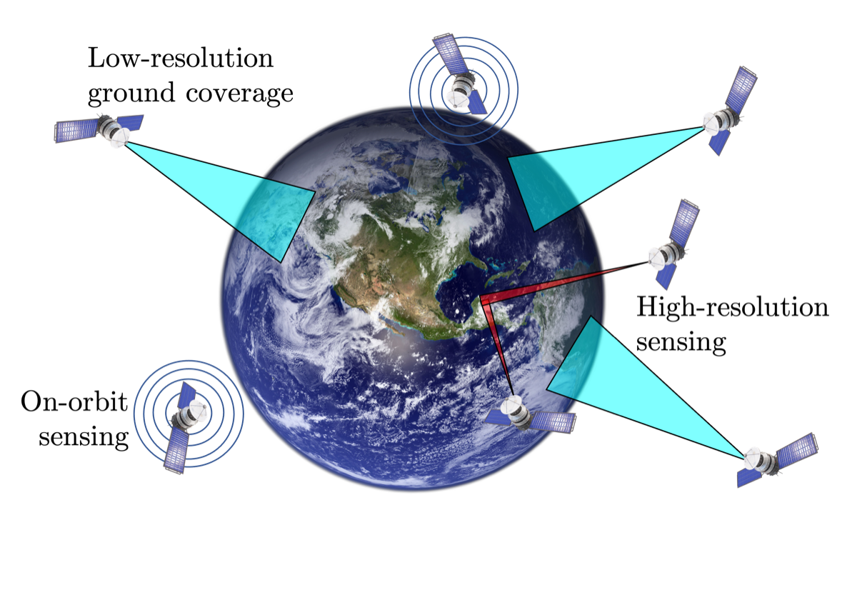
Fig. 1: It is often the case that only some of the satellites in a constellation are actively observing Earth at any given time. Furthermore, these satellites may be leveraged for multi-task missions.

3 Preliminaries and Background

In this section, we overview a number of relevant mathematical concepts for the ensuing algorithmic and theoretical developments.

3.1 Notation

We denote the set of nonnegative real numbers by $\mathbb{R}_{\geq 0}$, finite sets using calligraphic notation $\mathcal{S}$, random variables either by uppercase letters $X$ or lowercase Greek letters $\eta$, and the $n$-dimensional identity matrix by $I_{n}$. For a finite set $\mathcal{S}$, we denote its cardinality by $|\mathcal{S}|$ and its power set by $2^{\mathcal{S}}$. Finally, we compactly express a sequence of integers beginning at zero, e.g., $\{0,1,\ldots,n-1\}$, by $[n]$.

3.2 Submodular Maximization

In this section, we provide an overview of submodular maximization. We begin with the following definitions.

Definition 1 (Monotone nondecreasing).

A set function $f:2^{\mathcal{}X}\rightarrow\mathbb{R}$ is monotone nondecreasing if $f({\mathcal{}S})\leq f({\mathcal{}T})$ for all ${\mathcal{}S}\subseteq{\mathcal{}T}\subseteq{\mathcal{}X}$.

Definition 2 (Submodularity).

A set function $f:2^{\mathcal{}X}\rightarrow\mathbb{R}$ is submodular if

$$f({\mathcal{}S}\cup\{j\})-f({\mathcal{}S})\geq f({\mathcal{}T}\cup\{j\})-f({\mathcal{}T})$$ (1)

for all subsets ${\mathcal{}S}\subseteq{\mathcal{}T}\subset{\mathcal{}X}$ and $j\in{\mathcal{}X}\backslash{\mathcal{}T}$, where $f_{j}({\mathcal{}S})\vcentcolon=f({\mathcal{}S}\cup\{j\})-f({\mathcal{}S})$ is the marginal gain of adding $j$ to ${\mathcal{}S}$.

In the practical sense, the function $f$ is a performance objective, e.g., the additive inverse of the mean square error (MSE) [27, 13], and ${\mathcal{}X}$ is the set of all sensors, out of which a selection of suitable sensors will be made. It is commonplace to refer to this set ${\mathcal{}X}$ as the ground set. In this paper, we consider the setting where each sensor $j\in{\mathcal{}X}$ has a cost of selection $c_{j}\in\mathbb{R}_{\geq 0}$, and the total cost of a selection ${\mathcal{}S}$ is denoted by $c({\mathcal{}S})\vcentcolon=\sum_{j\in{\mathcal{}S}}c_{j}$. Note that when $c_{j}=1$ for all $j\in{\mathcal{}X}$ we have $c({\mathcal{}S})=|{\mathcal{}S}|.$ Let $\mathcal{C}\vcentcolon=\{c_{i}\,:\,i\in[|{\mathcal{}X}|]\}$ and define the ordered set $\bar{\mathcal{C}}\vcentcolon=\{\bar{c}_{i}\in\mathcal{C}\,:\,\bar{c}_{i}\leq\bar{c}_{j}\,\,\forall\,j\geq i\}$ such that $\bar{\mathcal{C}}=\mathcal{C}$.

For a monotone nondecreasing submodular function $f$ which is, in addition, normalized (i.e., $f(\emptyset)=0$), we are interested in solving the following budget-constrained combinatorial optimization problem:

$$\underset{{\mathcal{}S}\subseteq{\mathcal{}X}}{\text{maximize}}\quad f({\mathcal{}S})$$ (2)

$$\text{s.t.}\quad c({\mathcal{}S})\leq B,$$

where $B$ denotes the budget constraint value. By a reduction to the well-known set cover problem, (2) is known to be NP-hard [28, 8]. Note that when $c_{j}=1$ for all $j\in{\mathcal{}X}$, (2) reduces to the cardinality-constrained observation selection problem studied in [27, 13]. In this special case (i.e., in the cardinality-constrained problem), the simple Greedy algorithm that iteratively selects the remaining element with the highest marginal gain

$$j^{\ast}\in\operatorname*{arg\,max}_{j\in{\mathcal{}X}\backslash{\mathcal{}S}^{(i-1)}}f_{j}({\mathcal{}S}^{(i-1)}),$$ (3)

where ${\mathcal{}S}^{(i-1)}$ is the subset selected after the $(i-1)\textsuperscript{th}$ iteration, satisfies the optimal worst-case approximation ratio $f({\mathcal{}S}_{g})\geq\left(1-1/e\right)f({\mathcal{}S}^{\star})$, in which ${\mathcal{}S}_{g}$ is the subset selected by Greedy, and $\mathcal{S}^{*}$ is the optimal solution of (2) [9]. The simple extension of this result to the general, budget-constrained case is done through the Modified Greedy (MG) algorithm, which instead selects the remaining element with the highest the marginal-gain-to-cost ratio $f_{j}({\mathcal{}S}^{(i-1)})/c_{j}$ and adds it to the constructed solution as long as this addition does not violate the budget constraint. Reminiscent of the well-known result for the Greedy algorithm, MG is shown to achieve a $\frac{1}{2}(1-1/e)$ worst-case approximation ratio [11].

3.3 Weak Submodularity

In many sensor selection tasks, it is observed that $f$ is not strictly submodular but shows similar behavior to submodularity under certain conditions. Such functions are called weak submodular, with their distance to submodularity captured through the quantity known as the weak-submodularity constant (WSC) [29, 30, 31].

Definition 3 (Weak-submodularity constant).

The weak-submodularity constant (WSC) of a monotone nondecreasing set function $f$ is defined as

$$w_{f}\vcentcolon={\max_{({\mathcal{}S},{\mathcal{}T},i)\in\tilde{{\mathcal{}X}}}{f_{i}({\mathcal{}T})/f_{i}({\mathcal{}S})}},$$ (4)

where $\tilde{{\mathcal{}X}}=\{({\mathcal{}S},{\mathcal{}T},i)|{\mathcal{}S}\subseteq{\mathcal{}T}\subset{\mathcal{}X},i\in{\mathcal{}X}\backslash{\mathcal{}T}\}$.

Intuitively, the WSC of $f$ can be thought of as a measure of quantifying the violation of the submodularity property. Note that with this definition, we will call any set function $f$ weak submodular if it is monotone nondecreasing and its WSC is bounded. Further note that by Definition (2), a set function $f$ is submodular if and only if its WSC satisfies $w_{f}\leq 1$ [32, 33, 34]. We will generally assume throughout this work that $w_{f}\geq 1$ to emphasize that the objective function is typically weak submodular.

For a monotone nondecreasing function with a bounded WSC, we have the following proposition [31]:

Proposition 1.

Let $w_{f}\geq 1$ be the WSC of $f$, a normalized, monotone nondecreasing set function. Then, for two subsets ${\mathcal{}S}$ and ${\mathcal{}T}$ such that ${\mathcal{}S}\subset{\mathcal{}T}\subseteq{\mathcal{}X}$, it holds that

$$f({\mathcal{}T})-f({\mathcal{}S})\leq w_{f}\sum\nolimits_{j\in{\mathcal{}T}\backslash{\mathcal{}S}}f_{j}({\mathcal{}S}).$$ (5)

It is worth noting that the notion of weak submodularity is not yet standardized in literature. Alternative notions of weak submodularity exist, such as those presented in [32, 33, 29, 34]. Such notions may simplify the derivation of the approximation bounds depending on the application at hand (see e.g., [35, 30, 36, 31, 37]). Using the same notion of weak submodularity as the one in this work, [32] extends the theoretical results of [9] on the greedy algorithm to the case of weak submodular functions, obtaining a worst-case approximation ratio of $f({\mathcal{}S}_{g})\geq\left(1-e^{-1/w_{f}}\right)f({\mathcal{}S}^{\star})$.

4 High-Probability Approximation Factors for Greedy Algorithms with Random Sampling

Algorithm 1 Modified Randomized Greedy (MRG)

1:  Input: Weak submodular function $f$, ground set ${\mathcal{}X}$, budget constraint $B$, cost function $c$, sample cardinality $r_{i}$.

2:  Output: Subset ${\mathcal{}S}_{\operatorname{mrg}}\subseteq{\mathcal{}X}$ with $c({\mathcal{}S}_{\operatorname{mrg}})\leq B$.

3:  Initialize ${\mathcal{}S}^{(0)}=\emptyset$, $\mathcal{N}={\mathcal{}X}$, $i=0$

4:  while $\mathcal{N}\neq\emptyset$ do

5:     Form ${\mathcal{}R}^{(i)}$ by sampling $\min(r_{i},|\mathcal{N}|)$ elements from $\mathcal{N}$ uniformly at random.

6:     $j_{s}^{i}\in\operatorname*{arg\,max}_{j\in{\mathcal{}R}^{(i)}}\frac{f_{j}({\mathcal{}S}^{(i)})}{c_{j}}$

7:     if $c({\mathcal{}S}^{(i)})+c_{j_{s}^{i}}\leq B$ then

8:        ${\mathcal{}S}^{(i+1)}={\mathcal{}S}^{(i)}\cup\{j_{s}^{i}\}$

9:        $i\leftarrow i+1$

10:     end if

11:     $\mathcal{N}\leftarrow\mathcal{N}-\{j_{s}^{i}\}$

12:  end while

13:  Let $j_{\max}=\operatorname*{arg\,max}_{j\in{\mathcal{}X}}f(\{j\})$

14:  ${\mathcal{}S}_{\operatorname{mrg}}=\operatorname*{arg\,max}_{\mathcal{S}\in\{\mathcal{S}^{(i)},\{j_{\max}\}\}}f({\mathcal{}S})$

Greedy algorithms rely on a simple philosophy and are relatively straightforward to implement. In practice, however, it is usually undesirable to use the full Greedy algorithm which searches over the entire set of elements due to computational cost considerations. To overcome this computational burden, we propose two randomized greedy algorithms that, at each iteration, consider only a randomly sampled subset of the remaining elements in the ground set. As briefly explained in Section (1), these two algorithms will be used to tackle a budget-constrained weak submodular sensor selection task, and its dual formulation, i.e., a performance-constrained weak submodular sensor selection task. Furthermore, we derive performance guarantees that hold with high probability for both algorithms.

4.1 Budget-Constrained Sensor Selection

We start our high-probability analysis by studying how MRG, given in Algorithm (1), performs in budget-constrained weak submodular sensor selection tasks. To this end, we first need to address a fundamental question: how should we choose the size of the sampling sets ${\mathcal{}R}^{(i)}$ in each iteration? Note that we cannot directly utilize the strategies employed in the cardinality-constrained setting, i.e., setting $r_{i}=\frac{|{\mathcal{}X}|}{k}\log\frac{1}{\epsilon}$ according to [12, 27, 13], or adopt a progressively increasing schedule $r_{i}=\frac{|{\mathcal{}X}|}{k-i}\log\frac{1}{\epsilon}$ as outlined in [38, 39], where $k$ is the number of selected observations and $0<\epsilon<1$ is a parameter that is set at will by the user. To see the barrier in choosing the sampling size $r$, note that due to the budget constraint, it is not known a priori how many observations MRG will end up selecting given that $k$ is unknown. At this point, although intuitively $r_{i}$ should depend on $B$ and each sensor cost $c_{j}$, it may not be clear which strategy results in a non-trivial approximation bound. Hence, we adopt a constructive approach where we let $r_{i}=\frac{|{\mathcal{}X}|}{U}\log\frac{1}{\epsilon}$ for some $U>0$ and $0<\epsilon<1$ where $U$ is determined as part of our analysis.

We then proceed to follow and extend [40, 13], and begin with a simplifying assumption that views each iteration of MRG as an approximation to Modified Greedy for the budget-constraint formulation (2), which can be obtained from Algorithm (1) by setting the sample cardinality $r_{i}$ equal to $|{\mathcal{}X}|$. Essentially, Greedy is a special case of MRG in which the entire set of remaining sensors is sampled at each iteration. MRG is no longer able to consider every remaining element in the ground set at each iteration, so there is no guarantee of it successfully adding the remaining sensor whose marginal-gain-to-cost ratio is maximal as Greedy does. However, one can still view each iteration of MRG as adding an element satisfying

$$\frac{f_{j_{\operatorname{mrg}}^{i}}({\mathcal{}S}^{(i)})}{c_{j_{\operatorname{mrg}}^{i}}} \geq\eta^{(i+1)}\max_{j\in{\mathcal{}X}\backslash{\mathcal{}S}^{(i)}}\frac{f_{j}({\mathcal{}S}^{(i)})}{c_{j}}=\eta^{(i+1)}\frac{f_{j_{\operatorname{g}}^{i}}({\mathcal{}S}^{(i)})}{c_{j_{\operatorname{g}}^{i}}},$$ (6)

where the subscripts $\operatorname{mrg}$ and $\operatorname{g}$ refer to the sensor selected in the MRG and Greedy iterations, respectively, and $\eta^{(i)}\sim\mathcal{D}$ is a random variable drawn from some distribution $\mathcal{D}$ such that $\eta^{(i)}\in(0,1]$ for all $i$. Essentially, the key idea is that each iteration $i$ of MRG selects a sensor whose marginal-gain-to-cost ratio is at least $\eta^{(i+1)}$-times as good as the one selected by Greedy. In contrast to [40, 13], which consider i.i.d. draws of $\eta$’s for the cardinality-constrained scenario, we exploit the fact that each iteration of MRG is dependent on the selections made in the previous iterations. We then adopt the relaxed assumption that the stochastic process $\{\eta^{(i)}\}_{i=1}^{\infty}$ is a martingale [41].

Definition 4 (Martingale).

A stochastic process $\{Y_{i}\}_{i=1}^{\infty}$ is a martingale with respect to the stochastic process $\{X_{i}\}_{i=1}^{\infty}$ if, for all $n\in\mathbb{N}$, $\mathbb{E}[|Y_{n}|]<\infty$ and $\mathbb{E}[Y_{n+1}|X_{0},\ldots,X_{n}]=Y_{n}$.

Our martingale assumption is then formalized as follows:

Assumption 1 (Martingale).

The stochastic process $\{\eta^{(i)}\}_{i=1}^{\infty}$ is a martingale with respect to the stochastic process $\{\mathcal{S}^{(i)}\}_{i=0}^{\infty}$. That is, for all $i\in\mathbb{N},$ ${\mathbb{E}}[\eta^{(i+1)}|{\mathcal{}S}^{(0:i)}]=\eta^{(i)},$ where ${\mathcal{}S}^{(0:i)}\vcentcolon=\{{\mathcal{}S}^{(0)},\ldots,{\mathcal{}S}^{(i)}\}$ denotes the random collection of subsets obtained by MRG up to iteration $i$.

One may question the justifiability of adopting such an assumption. An informal yet intuitive characterization of a martingale is that it is a stochastic process that does not demonstrate a predictable drift[42]. In numerical experiments, this is indeed observed to be the case, rendering Assumption (1) realistic.

In the following, we use the next lemma to provide a concentration bound on the stochastic process $\{\eta^{(i)}\}_{i=1}^{\infty}$.

Lemma 1 (Azuma-Hoeffding inequality [41]).

Let $\{Y_{i}\}_{i=1}^{\infty}$ be a martingale with respect to $\{X_{i}\}_{i=1}^{\infty}$ such that $Y_{1}=\mu$. If there exists a sequence of real numbers $\beta_{i}$ such that for all $i\in\mathbb{N},\lvert Y_{i}-Y_{i-1}\rvert\leq\beta_{i}$, then for any $\lambda\in\mathbb{R}_{\geq 0}$,

$$\Pr\left(Y_{n}-\mu\leq-\lambda\right)\leq\exp\left(-\frac{{\color[rgb]{0,0,0}2}\lambda^{2}}{\sum_{i=1}^{n}\beta_{i}^{2}}\right).$$ (7)

Using Lemma (1) and Assumption (1), we now study the performance of MRG for weak submodular maximization subject to a budget constraint. We obtain the following theorem:

Theorem 1 (Performance of MRG).

Let $\{\eta^{(i)}\}_{i=1}^{\infty}$ satisfy Assumption (1) and the conditions of Lemma (1), where, for all $i\in\mathbb{N},$ ${\mathbb{E}}[\eta^{(i)}]\geq\mu$, for some $\mu\in\mathbb{R}_{\geq 0}$. Then, for any confidence parameter $0<\delta<1$, MRG constructs a solution ${\mathcal{}S}_{\operatorname{mrg}}$ to problem (2) such that

$$\frac{f({\mathcal{}S}_{\operatorname{mrg}})}{f({\mathcal{}S}^{\ast})}\geq\frac{1-\exp\left[-\frac{1}{w_{f}}\left(\mu-\frac{c_{\max}}{B}\sqrt{\frac{U}{2}\log\frac{1}{\delta}}\right)\right]}{2w_{f}^{2}},$$ (8)

with probability at least $1-\delta$, where ${\mathcal{}S}^{\ast}$ is an optimal solution, (8), $U$ is the smallest integer such that $\sum_{j=1}^{U}\bar{c}_{j}\geq B$ and $c_{max}\vcentcolon=\bar{c}_{|{\mathcal{}X}|}$.

Proof.

Sketch of Proof. The complete proof is stated in [15]. The aim is to prove the result assuming that the selection returned by the inner loop of MRG in Algorithm (1) is limited to the subset ${\mathcal{}S}^{(i_{v})}$ constructed up the to point before the condition in Line 7 of Algorithm (1) evaluates to false for the first time, since this will ensure that it will hold in the general case because of the monotone nondecreasing nature of $f$.

The subsequent applications of (4), (5), and (6), the use of induction over the iterations of the algorithm, and the invocation of Lemma (1) allow us to place an upper bound on the ratio $\nicefrac{{f({\mathcal{}S}^{(i_{v})})}}{{f({\mathcal{}S}^{\ast})}}$, completing the proof. ∎∎

One may wonder why lines 13 and 14 are present in the algorithm. The practical and intuitive reason is that these lines prevent certain adversarial scenarios where a single-element solution outperforms the greedily-constructed solution. More pragmatically, the full proof of Theorem (1) uses these lines in the establishment of the performance lower-bound.

Theorem (1) establishes a high-probability bound on the worst-case performance of MRG. Through observation of the right hand side of (8), one can see that the performance lower bound depends on several factors. Of these, $U$, $w_{f}$, $c_{\max}$ and $B$ are dictated by the problem itself and are not affected by the stochasticity of the algorithm. $\delta$ is the confidence parameter, which one sets a posteriori, to see the performance lower bound guaranteed at a certain probability. For instance, to see what the performance lower bound would be with at least $0.9$ probability, one would set $\delta=0.1$ and compute the right-hand side. Meaning, $\delta$ is also independent of the stochasticity of the algorithm. The only parameter which depends on the actual process of the algorithm is $\mu$, which one may think of as a lower bound on the expected values of all ${\mathbb{E}}[\eta^{(i)}]$ through the course of the algorithm. Even more intuitively, one can think of this value as a lower bound on the expected discrepancy between the performance of the standard Greedy procedure and MRG. When $c_{\max}\sqrt{U}\ll B$ (e.g., in the cardinality-constrained setting, where the cardinality constraint $k$ satisfies $\sqrt{k}\ll k)$, the right-hand side of (8) can be closely approximated by $\frac{1}{2w_{f}^{2}}(1-e^{-\mu/w_{f}})$. Additionally, if $f$ is submodular (for which $w_{f}=1$) and $\mu=1$, i.e., when $r_{i}=|{\mathcal{}X}|$, this last result reduces to $\frac{1}{2}(1-1/e)$, the approximation factor of Greedy [11]. It’s worth highlighting that the values of $c_{\max}$, $U$, and $B$ in equation (8) are either known beforehand or can be efficiently computed before running MRG. In contrast, $\omega_{f}$ and $\mu$ can be estimated through simulation. In certain specialized scenarios, such as minimizing the MSE in specific linear or quadratic observation models, upper bounds for $\omega_{f}$ can be found [13, 31].

The proof of Theorem (1) also provides an explanation as to the previous determination of the size of the sets ${\mathcal{}R}^{(i)}$ at each step of MRG. Considering that in the scenario with a cardinality constraint, the value of $k$ matches the size of ${\mathcal{}S}^{\ast}$, and given that $|{\mathcal{}S}^{\ast}|\leq U$, we suggest selecting $r_{i}=\frac{|{\mathcal{}X}|}{U}\log\frac{1}{\epsilon}$ sensors during each iteration of MRG. The results of $r_{i}$ on the runtime and the performance of the algorithm in a practical setting are demonstrated in Section (6), in Table (6) and Figure (3).

It might be counterintuitive to the reader that the stochastic process $\eta^{(i)}$ is unused in the algorithm. Put simply, $\eta^{(i)}$ describes a sequence of approximation ratios of the marginal-utility-per-cost performance of the stochastic greedy selection process to the utility marginal-utility-per-cost performance of the standard greedy selection process. Clearly, this is not a quantity that is meant to be (or can be) used in the design of the algorithm, since one would have no access to the actual values taken on by the sequence unless one ran a copy of the standard greedy selection process at each iteration, completely annulling the computational efficiency of MRG and essentially ending up twice as costly. Rather, $\eta^{(i)}$, (along with $\mu$, which is technically a statistic of $\eta^{(i)}$) is a natural byproduct resulting from the running of the algorithm, whose values are of no interest to us. The only quality we would like $\eta^{(i)}$ to possess is that it be a martingale, a reasonable assumption that appears to hold in many relevant practical settings.

Similarly, the confidence parameter $\delta$ is also unused in the algorithm. Indeed, the value of $\delta$ is only relevant in the theoretical guarantee of Theorem (1). Setting a value for $\delta$ allows us to observe the performance lower bound achievable for the approximation ratio achieved by MRG with probability at least $1-\delta$. For instance, one may observe that as $\delta$ approaches $0$, the right-hand side of (8) begins to attain negative values, and the performance lower bound guarantee becomes meaningless. In fact, for $\delta=\exp{(-2/U(\mu B/c_{\max})^{2})}$, the right-hand side is exactly equal to $0$, and for any value of $\delta$ less than or equal to this quantity, no guarantee is provided.

One must also not confuse the $\epsilon$ present in the setting of the size of the random sampling set $r_{i}=\frac{|{\mathcal{}X}|}{U}\log\frac{1}{\epsilon}$ with the confidence parameter $\delta$. There are many examples in literature of algorithms that provide guarantees in terms of an $(\epsilon,\delta)$ pair. However, in our setting, these parameters are only indirectly related, with $\epsilon$ determining the size $r_{i}$ of the sampling set, which in turn affects the value of $\mu$, which in turn affects the performance lower bound guaranteed by Theorem (1). Besides this, the $\epsilon$ and $\delta$ quantities are not related.

Algorithm 2 Dual Randomized Greedy (DRG)

1:  Input: Weak submodular function $f$, ground set ${\mathcal{}X}$, performance threshold $A$, cost function $c$, sample cardinality $r_{i}$.

2:  Output: Subset ${\mathcal{}S}_{\operatorname{drg}}\subseteq{\mathcal{}X}$ with $f({\mathcal{}S}_{\operatorname{drg}})\geq A$.

3:  Initialize ${\mathcal{}S}^{(0)}=\emptyset$, $\mathcal{N}={\mathcal{}X}$, $i=0$

4:  while $f({\mathcal{}S}^{(i)})<A$ do

5:     Form ${\mathcal{}R}^{(i)}$ by sampling $\min(r_{i},|\mathcal{N}|)$ elements from $\mathcal{N}$ uniformly at random.

6:     $j_{s}^{i}\in\operatorname*{arg\,max}_{j\in{\mathcal{}R}^{(i)}}\frac{f_{j}({\mathcal{}S}^{(i)})}{c_{j}}$

7:     ${\mathcal{}S}^{(i+1)}={\mathcal{}S}^{(i)}\cup\{j_{s}^{i}\}$

8:     $i\leftarrow i+1$

9:     $\mathcal{N}\leftarrow\mathcal{N}-\{j_{s}^{i}\}$

10:  end while

11:  Set ${\mathcal{}S}_{\operatorname{drg}}={\mathcal{}S}^{(L)}$, $L=i$

4.2 Performance-Constrained Sensor Selection

We now establish a high-probability bound for the performance of Dual Randomized Greedy (DRG), given in Algorithm (2), for the dual problem of (2), where we aim to satisfy a performance threshold while minimizing the total cost of the selected sensors. This problem is formally expressed as follows:

$$\underset{{\mathcal{}S}\subseteq{\mathcal{}X}}{\text{minimize}}\quad c({\mathcal{}S})$$ (9)

$$\text{s.t.}\quad f({\mathcal{}S})\geq A,$$

for some performance threshold $A\in\mathbb{R}_{\geq 0}$. Note that when $A=f({\mathcal{}X})$ and $f$ is submodular, (9) corresponds exactly to the well-known submodular set covering problem [10]. In that case, the standard Greedy algorithm, which again represents a special case of Algorithm (2) in which $r_{i}=|{\mathcal{}X}|$, obtains the optimal approximation factor [10], given by

$$\frac{c({\mathcal{}S}_{\operatorname{g}})}{c({\mathcal{}S}^{\ast})}\leq 1+\log\left(\frac{f_{j}({\mathcal{}S}^{(0)})}{f_{j}({\mathcal{}S}^{(L-1)})}\right)\leq 1+\log\frac{M}{m},$$ (10)

where $L$ denotes the total number of iterations taken by Greedy until a solution is returned, $M\vcentcolon=\max_{j\in{\mathcal{}X}}f_{j}(\emptyset)$, and $\quad m\vcentcolon=\min_{j\in{\mathcal{}X}\backslash{\mathcal{}S}^{(L-1)}}f_{j}({\mathcal{}S}^{(L-1)}).$ Under the same observation made in (6), we establish that DRG achieves a similar approximation factor with high probability.

Theorem 2 (Performance of DRG).

Let $\{\eta^{(i)}\}_{i=1}^{\infty}$ satisfy Assumption (1) and the conditions of Lemma (1), where, for all $i\in\mathbb{N},{\mathbb{E}}[\eta^{(i)}]\geq\mu$, for some $\mu\in\mathbb{R}_{\geq 0}$. Then, for any confidence parameter $0<\delta<1$, DRG finds a solution ${\mathcal{}S}_{\operatorname{drg}}$ to problem (9) such that, with probability at least $1-\delta$,

$$\frac{c({\mathcal{}S}_{\operatorname{drg}})}{c({\mathcal{}S}^{\ast})} \leq\frac{{w_{f}}}{\mu}\left[1+(L-1)\log w_{f}+\log\frac{M}{m}\right]$$ (11)

$$\qquad+\frac{1}{\mu c({\mathcal{}S}^{\ast})}\sqrt{\frac{1}{2}\log\frac{1}{\delta}c^{2}({\mathcal{}S}_{\operatorname{drg}})},$$

where ${\mathcal{}S}^{\ast}$ is an optimal solution, $L\leq|{\mathcal{}X}|$ is the number of iterations required by DRG until termination, and $c^{2}({\mathcal{}S}_{\operatorname{drg}})\vcentcolon=\sum_{j\in{\mathcal{}S}_{\operatorname{drg}}}c^{2}_{j}.$

Proof.

Sketch of Proof. The complete proof is stated in [15]. Here, the fundamental idea is to consider a relaxation of Problem (9), which brings it into the domain of linear programming. The solutions to this relaxation can then be shown, by application of the weak duality theorem, to be solutions to the original problem.

Lastly, Lemma (1) is invoked to obtain the high-probability guarantee, completing the proof. ∎∎

Recall that the standard Greedy algorithm is a special case of DRG in which $r_{i}=|{\mathcal{}X}|$. In this case, we can set $\mu=\delta=1$. Using the result of Theorem (2), we directly obtain that

$$\frac{c({\mathcal{}S}_{\operatorname{drg}})}{c({\mathcal{}S}^{\ast})}\leq w_{f}\left[1+(L-1)\log w_{f}+\log\frac{M}{m}\right],$$ (12)

which extends the result of [10] to the general setting of performance-constrained weak submodular optimization that we have formulated in (9), and generalizes the result established in [43] for the unit-cost case. This last result naturally reduces to (10) for the case that $f$ is a submodular function, for which $w_{f}=1$. Much like the performance bound of MRG, the upper bound on the approximation ratio of DRG is dependent on terms that arise from the problem setting as well as those that are due to the stochasticity of the algorithm. In particular, $w_{f}$, $c(S^{\ast})$ and $m$ are parameters that depend on the nature of the problem at hand and are independent of the algorithm. $\mu$ and $\delta$ serve very similar purposes to those in the case of MRG, and are already discussed thoroughly in that section. $M$ is interesting in that it depends both on the nature of the problem and the objective functions, and also the selections made by the algorithm up to the $(L-1)^{\text{th}}$ step. Finally, $L$ is a parameter that essentially indicates how long the algorithm runs until a solution is found, and depends entirely on the course of the algorithm. Lastly, it’s worth noting that the parameter $M$ can also be calculated efficiently before starting the DRG process, whereas the values of $L$ and $m$ are determined during the execution of the algorithm.

5 A Randomized Method for Worst-Case Robustness

In this section, we study the application of the DRG algorithm to the solution of a standard formulation of the robust (weak) submodular maximization problem under the budget constraint proposed in [44]. We assume that we are given a finite collection of weak submodular, monotone nondecreasing, and normalized functions $f^{i},f^{2},\ldots,f^{n}$. We formulate the robust problem as follows:

$$\begin{split}&\underset{{\mathcal{}S}\subseteq{\mathcal{}X}}{\text{maximize}}\phantom{k}\underset{i\in[n]}{\text{minimize}}\quad f^{i}(S)\\ &\text{s.t. }\quad c({\mathcal{}S})\leq B.\end{split}$$ (13)

We can visualize this problem as such: we have $n$ distinct performance objectives that we want to maximize by selecting the optimal subset ${\mathcal{}S}\subseteq{\mathcal{}X}$. Since we expect a reasonable performance with respect to all of these objectives, we want to maximize the worst-performing one, all the while staying under a given budget constraint $B\in\mathbb{R}_{\geq 0}$. In [44], the Submodular Saturation Algorithm (SSA) is proposed, which solves a relaxation of Problem (13) in the setting where all of the objectives are submodular and a cardinality constraint is posed. SSA is presented in Algorithm (3).

Algorithm 3 Submodular Saturation Algorithm (SSA)[44]

Input: Finite collection of monotone nondecreasing submodular functions $f^{1},\ldots f^{n}$, ground set ${\mathcal{}X}$, cardinality constraint $K\in\mathbb{N}$, relaxation parameter $\alpha\geq 1$
   Output: Solution set ${\mathcal{}S}$

1:  $k_{m}\leftarrow 0$

2:  $k_{M}\leftarrow\min_{i}f^{i}({\mathcal{}X})$

3:  ${\mathcal{}S}\leftarrow\emptyset$

4:  while $k_{M}-k_{m}\geq 1/n$ do

5:     $k\leftarrow(k_{M}-k_{m})/2$

6:     Define $\bar{f}_{(k)}({\mathcal{}S})\leftarrow\frac{1}{n}\sum_{i=1}^{n}\min\{f^{i}({\mathcal{}S}),k\}$

7:     $\hat{{\mathcal{}S}}\leftarrow\textsc{Greedy}(\bar{f}_{(k)},k)$

8:     if $\lvert\hat{{\mathcal{}S}}\rvert>\alpha K$ then

9:        $k_{M}\leftarrow k$

10:     else

11:        $k_{m}\leftarrow k$

12:        ${\mathcal{}S}\leftarrow\hat{{\mathcal{}S}}$

13:     end if

14:  end while

To facilitate the following discussion, we now provide a brief description of SSA. Given a finite collection of normalized, monotone nondecreasing submodular functions $f^{1},\ldots f^{n}$, a cardinality constraint $K\in\mathbb{N}$, and a relaxation parameter $\alpha\geq 1$, SSA constructs a solution ${\mathcal{}S}\subseteq{\mathcal{}X}$ such that $f^{i}({\mathcal{}S})\geq k$ for a certain $k>0$ and $\lvert{\mathcal{}S}\rvert\leq\alpha K$. Hence, it solves a relaxation of Problem (13), where the budget constraint has been reduced to a cardinality constraint and has been relaxed by a factor of $\alpha$.

SSA leverages two useful facts. The first is that when $f$ is a submodular function, so is the truncated function given by $f_{(k)}\vcentcolon=\min\{f^{i}(A),k\}$ [44], which we call $f$ truncated at $k$. The second is that the nonnegative weighted sum (and hence the arithmetic mean) of submodular functions is again submodular [44]. The algorithm then truncates the input functions $f^{1},\ldots,f^{n}$ and averages them, producing the submodular function $\bar{f}_{(k)}$. It adaptively decides on the truncation value $k$ by doing a line search over the feasible values of $k$, and outputs a solution ${\mathcal{}S}\subseteq{\mathcal{}X}$ with $f^{i}({\mathcal{}S})\geq k$ for all $i\in[n]$, where $k$ is the highest value found by the line search procedure. As can be seen in Line 7, SSA makes use of the Greedy as a subroutine. The aim of this section is twofold: to extend the result given in [44] using Greedy to one using the computationally cheaper, randomized version of DRG, and to further generalize the result to the case involving weak submodular functions and a more complex budget constraint with nonuniform costs instead of the simpler cardinality-constrained setting.

Now, with regard to SSA, we have the following theoretical guarantee:

Theorem 3 (Performance of SSA[44]).

For any cardinality constraint $K\in\mathbb{N}$, SSA finds a solution $\hat{{\mathcal{}S}}$ to a relaxation of Problem (13), where $f^{i}$ are submodular for all $i\in\{1,\ldots,n\}$, such that

$$\min_{i\in[n]}f^{i}(\hat{{\mathcal{}S}})>\max_{{\mathcal{}S}\subseteq{\mathcal{}X},c({\mathcal{}S})\leq B}\min_{i\in[n]}f^{i}({\mathcal{}S})$$ (14)

and $c(\hat{{\mathcal{}S}})\leq\alpha B,$ for $\alpha=1+\log(\max_{j\in{\mathcal{}X}}\sum_{i=1}^{n}f^{i}(\{j\})$.

The above result relies on the following lemma concerning the Greedy algorithm [45]:

Lemma 2.

Given a submodular function $f$ over a ground set ${\mathcal{}X}$, and a feasible performance threshold value $k$, the Greedy algorithm produces a solution $\hat{{\mathcal{}S}}$ such that

$$\dfrac{\lvert\hat{S}\rvert}{\lvert{\mathcal{}S}^{\ast}\rvert}\leq 1+\log\max_{j\in{\mathcal{}X}}f(\{j\}),$$ (15)

where ${\mathcal{}S}^{\ast}$ is an optimal solution (i.e., ${\mathcal{}S}^{\ast}=\arg\!\min\{\lvert{\mathcal{}S}\rvert:f({\mathcal{}S})\geq k\}$).

With this result, it becomes clear how Theorem (3) provides this guarantee: since Greedy is guaranteed to return a solution $\hat{{\mathcal{}S}}$ such that $\lvert\hat{{\mathcal{}S}}\rvert/\lvert{\mathcal{}S}^{\ast}\rvert\leq 1+\log\max_{j\in{\mathcal{}X}}f(\{j\})$, we may set our relaxation parameter $\alpha$ in SSA to exactly this upper bound on the right-hand side. Doing so, we know that if GPC fails to return a solution for a given performance threshold $k$, then that $k$ must be infeasible. Consequently, it only remains to find the highest $k$ value that is feasible, which is achieved by a simple line search procedure. For the line search, the values for the interval to be searched at the current iteration are set in Lines 1 and 2 and are updated after each run of the Greedy subroutine. If the Greedy subroutine fails to return a solution, we know that the most recent $k$ value provided was infeasible, so we update the higher end of our search interval to that value (Line 9). If, on the other hand, the Greedy subroutine did return a solution, then the most recent $k$ value provided was feasible. This case does not preclude the possibility that there is yet another, higher $k$ value which is feasible, so we continue the line search by updating the lower end of our search interval to this value (Line 11).

It may not be readily apparent how giving the average of the truncated $f^{1},\ldots,f^{n}$, i.e., $\bar{f}_{(k)}$ as input into the Greedy subroutine guarantees that the solution $\hat{{\mathcal{}S}}$ returned by Greedy satisfies $f^{1}(\hat{{\mathcal{}S}}),\ldots,f^{n}(\hat{{\mathcal{}S}})\geq k$. It suffices to see that the average of these functions $f^{1}(\hat{{\mathcal{}S}}),\ldots,f^{n}(\hat{{\mathcal{}S}})$ truncated at $k$ is equal to $k$ if and only if $f^{1}(\hat{{\mathcal{}S}}),\ldots,f^{n}(\hat{{\mathcal{}S}})\geq k$. In other words, even if a single $f^{j}(\hat{{\mathcal{}S}})<k$, this would make its truncated counterpart $f^{j}_{(k)}(\hat{S})<k,$ and hence even if for all other $i\neq j,f^{i}(\hat{{\mathcal{}S}})\geq k$ holds, their average would not satisfy the performance threshold, i.e., $\bar{f}_{(k)}=\frac{1}{n}\sum_{i=1}^{n}f^{i}_{(k)}(\hat{{\mathcal{}S}})<k$.

Before directly analyzing the use of DRG instead of Greedy, there yet remains a gap to be bridged between the setting of [44] and this work, that is, the consideration of weak submodular functions instead of proper submodular functions. To derive a result similar to Theorem (3) in the case of weak submodular functions, we need to demonstrate that averaging and truncation preserve weak submodularity as it does in the case of submodularity. This preservation is indeed the case, as shown in the following two lemmas.

Lemma 3.

Let $f^{1},\ldots,f^{n}$ be weak submodular with WSCs $w_{f^{1}},\ldots,w_{f^{n}}<\infty.$ Any nonnegative weighted sum $\bar{f}$ of $f^{1},\ldots f^{n}$ is also weak submodular, with $w_{\bar{f}}<\infty$.

In particular, note that this result implies that the average of a finite number of weak submodular functions is yet again a weak submodular function.

We now show a similar result for the truncation of a weak submodular function.

Lemma 4.

Let $f$ be a weak submodular function, i.e., $w_{f}<\infty.$ Then, the truncation of $f$ at $k\leq 0$, which is denoted $f_{(k)}({\mathcal{}S})\vcentcolon=\min\{f({\mathcal{}S}),k\},$ with the convention that if $f_{(k)_{i}}(T)/f_{(k)_{i}}(S)=\nicefrac{{0}}{{0}},$ then $f_{(k)_{i}}(T)/f_{(k)_{i}}(S)=0,$ is a weak submodular function with $w_{f_{(k)}}<\infty$.

Proof.

By our definition of weak submodularity, any set function that is monotone nondecreasing and has bounded WSC is weak submodular, so we first show that $f_{(k)}$ is monotone nondecreasing. Now, for any pair of sets ${\mathcal{}S}\subseteq{\mathcal{}T}$ where $f({\mathcal{}S}),f({\mathcal{}T})\leq k$, $f_{(k)}({\mathcal{}S})=f({\mathcal{}S})\leq f({\mathcal{}T})=f_{(k)}({\mathcal{}T})$. For any pair of sets ${\mathcal{}S}\subseteq{\mathcal{}T}$ where $f({\mathcal{}S})\leq k$ and $f({\mathcal{}T})>k$, $f_{(k)}({\mathcal{}S})=f({\mathcal{}S})\leq k=f_{(k)}({\mathcal{}T}).$ Finally, for any pair of sets ${\mathcal{}S}\subseteq{\mathcal{}T}$ where $f({\mathcal{}S}),f({\mathcal{}T})>k$, $f_{(k)}({\mathcal{}S})=k=f_{(k)}({\mathcal{}T})$. Hence, $f_{(k)}$ is monotone nondecreasing.

Now, let us recall the following definition:

$$w_{f_{(k)}}\vcentcolon=\max_{({\mathcal{}S},{\mathcal{}T},i)\in\tilde{{\mathcal{}X}}}f_{(k)_{i}}({\mathcal{}T})/f_{(k)_{i}}({\mathcal{}S}).$$ (16)

Say that this maximum is attained at $({\mathcal{}S}_{0},{\mathcal{}T}_{0},i_{0}).$ Due to the monotone nondecreasing nature of $f_{(k)},$ we have that

$$f_{(k)}({\mathcal{}S}_{0})\leq f_{(k)}({\mathcal{}T}_{0})\leq f_{(k)}({\mathcal{}T}_{0}\cup\{i_{0}\}),$$ (17)

and

$$f_{(k)}({\mathcal{}S}_{0})\leq f_{(k)}({\mathcal{}S}_{0}\cup\{i_{0}\})\leq f_{(k)}({\mathcal{}T}_{0}\cup\{i_{0}\}).$$ (18)

Let us say that a truncated function $f_{(k)}$ is saturated at ${\mathcal{}S}$ if $f_{(k)}({\mathcal{}S})=k$. In light of these inequalities, the remainder of the proof reduces to checking whether or not $f_{(k)}$ is saturated at each of ${\mathcal{}S}_{0},{\mathcal{}T}_{0},{\mathcal{}S}_{0}\cup\{i_{0}\},$ and ${\mathcal{}T}_{0}\cup\{i_{0}\}$. For instance, if $f_{(k)}$ is saturated at ${\mathcal{}S}_{0},$ we have, by convention, $w_{f_{(k)}}=\nicefrac{{0}}{{0}}=0<\infty.$ If, on the other hand, $f_{(k)}$ is not saturated at ${\mathcal{}S}_{0}$ but at ${\mathcal{}T}_{0},$ we have, $w_{f_{(k)}}=0<\infty.$ Investigating the rest of the valid configurations, we obtain

$$w_{f_{(k)}}\in\mathcal{W}\vcentcolon=\left\{0,\frac{k-f({\mathcal{}T}_{0})}{k-f({\mathcal{}S}_{0})},\frac{k-f({\mathcal{}T}_{0})}{f_{{(k)}_{i_{0}}}({\mathcal{}S}_{0})},w_{f}\right\}.$$ (19)

It is important to note that $f_{(k)_{i_{0}}}({\mathcal{}S}_{0})=f_{(k)}({\mathcal{}S}_{0}\cup\{i_{0}\})-f_{(k)}({\mathcal{}S}_{0})$ is obtained only in the case where $f_{(k)}$ is not saturated at ${\mathcal{}S}_{0}\cup\{i_{0}\}$ (and hence at ${\mathcal{}S}_{0}$), which means that $f_{(k)}({\mathcal{}S}_{0}\cup\{i_{0}\})=f({\mathcal{}S}_{0}\cup\{i_{0}\})$ and $f_{(k)}({\mathcal{}S}_{0})=f({\mathcal{}S}_{0}).$ Hence, it must be that $f_{(k)}({\mathcal{}S}_{0}\cup\{i_{0}\})\neq f_{(k)}({\mathcal{}S}_{0}),$ as otherwise, $({\mathcal{}S}_{0},{\mathcal{}T}_{0},i_{0})$ would have been a maximizer of $w_{f}\vcentcolon={\max_{({\mathcal{}S},{\mathcal{}T},i)\in\tilde{{\mathcal{}X}}}{f_{i}({\mathcal{}T})/f_{i}({\mathcal{}S})}},$ making $w_{f}=\infty,$ violating the premise that $w_{f}<\infty.$ We conclude, then, that every element of $\mathcal{W}$ is a finite value, i.e., $w_{f_{(k)}}<\infty.$ ∎∎

With these two results, we are now ready to present Randomized Weak Submodular Saturation Algorithm (Random-WSSA). To summarize, Random-WSSA uses the main body of SSA, with the Greedy subroutine replaced by the randomized equivalent of DRG, and furthermore, works in the presence of weak submodular functions. The full algorithm is presented in Algorithm (4).

Algorithm 4 Randomized Weak Submodular Saturation Algorithm (Random-WSSA)

Input: Finite collection of monotone nondecreasing weak submodular functions $f^{1},\ldots f^{n}$, ground set ${\mathcal{}X}$, budget constraint $B\in\mathbb{R}_{\geq 0}$, cost function $c$, relaxation parameter $\alpha\geq 1$
   Output: Solution set ${\mathcal{}S}$

1:  $k_{m}\leftarrow 0$

2:  $k_{M}\leftarrow min_{i}f^{i}({\mathcal{}X})$

3:  ${\mathcal{}S}\leftarrow\emptyset$

4:  while $k_{M}-k_{m}\geq 1/n$ do

5:     $k\leftarrow(k_{M}-k_{m})/2$

6:     Define $\bar{f}_{(k)}({\mathcal{}S})\leftarrow\frac{1}{n}\sum_{i=1}^{n}\min\{f^{i}({\mathcal{}S}),k\}$

7:     $\hat{{\mathcal{}S}}\leftarrow\operatorname{DRG}(\bar{f}_{(k)},k)$

8:     if $c(\hat{{\mathcal{}S}})>\alpha B$ then

9:        $k_{M}\leftarrow k$

10:     else

11:        $k_{m}\leftarrow k$

12:        ${\mathcal{}S}\leftarrow\hat{{\mathcal{}S}}$

13:     end if

14:  end while

From the preceding results, it is straightforward to show how the theoretical guarantee for Random-WSSA is established. We formalize this result in the following theorem.

Theorem 4.

Suppose the conditions of Theorem (2) hold. Then, for any confidence parameter $0<\delta<1$, and for any budget constraint $B\in\mathbb{R}_{\geq 0}$, Random-WSSA finds a solution $\hat{{\mathcal{}S}}$ to a relaxation of Problem (13), where $f^{i}$ are weak submodular, i.e., are monotone nondecreasing with WSCs $w_{f^{i}}<\infty$ for all $i\in[n]$, such that with probability at least $(1-\delta)^{P}$,

$$\min_{i\in[n]}f^{i}(\hat{{\mathcal{}S}})>\max_{c({\mathcal{}S})\leq B}\min_{i\in[n]}f^{i}({\mathcal{}S})$$ (20)

and $c(\hat{{\mathcal{}S}})\leq\alpha B,$ for

$$\begin{split}\alpha&=\dfrac{w_{\bar{f}_{(k)}}}{\mu}\left[1+(L-1)\log(w_{\bar{f}_{(k)}})+\log\dfrac{M}{m}\right]\\ &+\frac{1}{\mu c({\mathcal{}S}^{\ast})}\sqrt{\frac{1}{2}\log\frac{1}{\delta}c^{2}(\hat{{\mathcal{}S}})},\end{split}$$ (21)

where $L\leq|{\mathcal{}X}|$ is the maximum number of iterations required by DRG until termination throughout all iterations of Random-WSSA, $P$ is the number of iterations required by Random-WSSA until termination, $c^{2}({\mathcal{}S})=\sum_{j\in{\mathcal{}S}}c_{j}^{2},M=\max_{j\in{\mathcal{}X},i\in[n]}f^{i}(\{j\}),$ and $m=\min_{j\in{\mathcal{}X},i\in[n]}f^{i}_{j}({\mathcal{}X}\setminus\{j\}).$

Proof.

The proof follows immediately from Theorem (2), and Lemmas (1), (3), (4). Note that since the DRG subroutine is run $P$ times throughout the execution of Random-WSSA, and that these runs are statistically independent random events, the high-probability guarantee $(1-\delta)$ is raised to the exponent $P$, to account for each of the $P$ times that DRG must succeed in returning a solution. ∎∎

To provide concrete values for the setting of $\alpha$, note that the upper bound in Theorem (2) is given in terms of the quantities $c^{2}(\hat{{\mathcal{}S}})$ and $c({\mathcal{}S}^{*})$. One may upper-bound the first term instead by $c^{2}({\mathcal{}X})$ and lower-bound the second tern instead by $1$. In case $c({\mathcal{}S}^{\ast})<1$, one must only scale the cost value $c_{j}$ of every element $j\in{\mathcal{}X}$ and the budget $B$ by the factor $1/c_{\text{min}}$, where $c_{\text{min}}=\min_{j\in{\mathcal{}X}}c_{j}.$ Doing so ensures that for all ${\mathcal{}S}\subseteq{\mathcal{}X},c({\mathcal{}S})\geq 1$, and in particular, $c({\mathcal{}S}^{\ast})\geq 1$, after which we can safely do the lower-bounding by $1$. However, in practical settings, one usually does not have to resort to such strategies, as experimental results demonstrate that Random-WSSA very frequently succeeds to construct solutions for the nonrelaxed version of the problem, i.e., with $\alpha=1.$

6 Numerical Examples

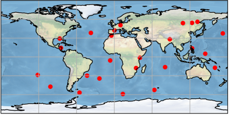
Fig. 2: Locations of the $25$ randomly-selected atmospheric points of interest.

Table 1: Average MRG solution time in seconds (Algorithm (1)) over the simulation horizon for various $r_{i}$ and budgets $B$. Note that $r_{i}=240$ corresponds to using the entire ground set, i.e., the standard Greedy algorithm.

—c——c—c—c—c— $B=25$ $B=50$ $B=75$ $B=100$
$r_{i}=60$ $1.52$ $1.59$ $1.59$ $1.58$
$r_{i}=120$ $2.93$ $2.95$ $3.03$ $3.01$
$r_{i}=180$ $3.96$ $3.96$ $3.98$ $3.96$
$r_{i}=240$ $4.33$ $4.33$ $4.39$ $4.34$

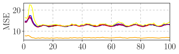
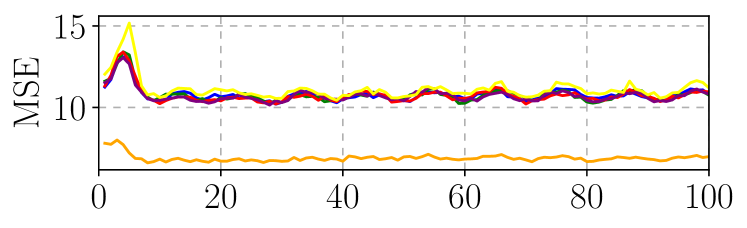
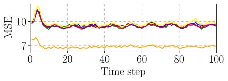
Fig. 3: Total mean-square errors (MSE) over time for various $r_{i}$ and $B$. From top to bottom are the plots for $B=25$, $50$, $75$, and $100$, respectively. Performance of using the entire set of satellites as well as that of picking the highest elements in terms of marginal-gain-to-cost ratio with respect to the empty set until the budget constraint is met (which we name Top-K) are included as benchmark values. Note that $r_{i}=240$ corresponds to using the entire ground set, i.e., the standard Greedy algorithm.

Table 2: Average MRG MSE values incurred (Algorithm (1)) over the simulation horizon for various $r_{i}$ and budgets $B$. Average MSE values for using the entire set and utilizing a Top-K approach are included as benchmarks. Note that $r_{i}=240$ corresponds to using the entire ground set, i.e., the standard Greedy algorithm.

—c——c—c—c—c— $B=25$ $B=50$ $B=75$ $B=100$
$r_{i}=60$ $17.73$ $12.93$ $10.78$ $9.52$
$r_{i}=120$ $17.27$ $12.82$ $10.78$ $9.52$
$r_{i}=180$ $17.33$ $12.83$ $10.75$ $9.50$
$r_{i}=240$ $17.23$ $12.81$ $10.74$ $9.51$
Entire set $6.89$ $6.89$ $6.89$ $6.89$
Top-K $19.39$ $13.52$ $11.12$ $9.74$

We now corroborate our theoretical results on the proposed algorithms for tasks involving sensor selection in the context of LEO satellite constellations. We consider a Walker-Delta constellation parameterized by $i:T/P/f$, where $i$ is the orbit inclination, $T$ is the number of satellites, $P$ is the number of unique orbits, and $f$ is the relative spacing between the satellites [46]. The constellation altitude is $2000$km, and the satellites are assumed to remain Earth-pointing with conical field-of-views of angle $\nicefrac{{\pi}}{{3}}$.

6.1 Sensor Selection for Atmospheric Monitoring with MRG

Consider a LEO satellite constellation parameterized by $60^{\mathrm{o}}:240/12/1$ performing atmospheric sensing over a set of $25$ randomly-instantiated points of interest, as shown in Figure (2). We simulate the conditions at each point $\mathbf{x}_{p}(t)=[x_{p}(t),y_{p}(t),z_{p}(t)]^{\top}$ with the Lorenz 63 model [47], a simplified model of atmospheric convection, in which $x_{p}$ is proportional to the rate of convection while $y_{p}$ and $z_{p}$ are proportional to the horizontal and vertical temperature variation, respectively. Precisely, the dynamics at each point are described by

$$\dot{\mathbf{x}}_{p}=\begin{bmatrix}\dot{x}_{p}\\ \dot{y}_{p}\\ \dot{z}_{p}\end{bmatrix}=\kappa\begin{bmatrix}\sigma(y_{p}-x_{p})\\ x_{p}(\rho-z_{p})-y_{p}\\ x_{p}y_{p}-\beta z_{p}\end{bmatrix}+\omega_{p},$$

where $\kappa,\sigma,\rho,\beta\in\mathbb{R}$. Note that we have omitted the time $t$ for notational clarity. For this simulation, we choose values of $\kappa=0.005,\sigma=10$, $\beta=\frac{8}{3}$, and $\rho=28$. With this selection of parameters, the system exhibits chaotic behavior. Furthermore, $\omega_{p}\sim\mathcal{N}([0,0,0]^{\top},\Sigma_{\omega_{p}})$ is a zero-mean Gaussian process modeling the noise. For this simulation, we set $\Sigma_{\omega_{p}}=0.1I_{3}$.

We assign the $n^{th}$ satellite a cost $c_{n}$ uniformly at random from the interval $[1,2]$. At each time step of the simulation, the decision-maker aims to make an optimal selection of a subset of the satellites to minimize the MSE of the estimated atmospheric reading, which is known to be a weak submodular function [27], while staying under a given budget constraint $B$. In our setting, each time step of the simulation corresponds to $\Delta t=60$s of time in the simulation. The budget constraint $B$ itself could practically be used to model several real-life limitations, e.g., communication costs between the satellites and the decision-maker or the operational cost of obtaining a reading from a specific satellite. In a real scenario, the cost values of each satellite should be tailored to the specific mission parameters.

The decision-maker uses an unscented Kalman Filter [48] to estimate the atmospheric state at each point of interest, using the measurement model

$$\mathbf{z}_{p,n}^{s}=\mathbf{1}_{p,n}^{s}\mathbf{x}_{p}(s\Delta t)+\nu_{p,n}^{s},$$ (22)

where $\mathbf{z}_{p,n}^{s}\in\mathbb{R}^{3}$ is the $n^{th}$ satellite’s observation of point $p$ at step $s$, $\mathbf{1}_{p,n}^{s}$ is an indicator function equal to $1$ if $p$ is in the field-of-view of the $n^{th}$ satellite at step $s$ and $0$ otherwise, and $\nu_{p,n}^{s}\sim{\mathcal{}N}([0,0,0]^{\top},\Sigma_{\nu_{p}})$ is Gaussian measurement noise with $\Sigma_{\nu_{p}}=2I_{3}$. As demonstrated in [27], the objective of minimizing the MSE of the estimator obtained from the selection of satellites can be directly modeled as maximizing a monotone nondecreasing weak submodular performance objective.

We test several sampling set sizes $r_{i}$ and budgets $B$, simulating the estimation task over a horizon of $100$ time steps. At each time step, we update the satellite positions and atmospheric conditions. Subsequently, we run MRG at each time step to reconstruct a feasible and optimal selection of satellites to use for atmospheric reading. As benchmarks, we include two additional methods of selecting satellites. One consists of not making a selection at all and using the entire constellation of satellites at all times. This demonstrates the ideal scenario of the lowest achievable MSE value at each step, however, it also always incurs the highest cost possible, violating any meaningful constraint on the budget. Additionally, we include the method which we denote “Top-K”. This entails sorting the entire set of satellites in decreasing order of marginal-gain-to-cost ratio and then sequentially adding them to the selection as long as they do not violate the budget constraint. Figure (3) shows the resulting MSE throughout the simulation for different combinations of $r_{i}$ and $B$ values. Table (6) shows the average wall-clock computation time of MRG for each combination. Table (6) shows the average MSE values over the entire time horizon of the simulation incurred by different methods for varying values of $r_{i}$ and $B$, effectively displaying the results in Figure (3) in tabulated format. As would be expected, increasing the budget value $B$ allows MRG to add additional satellites whose field-of-view may contain additional points of interest, increasing the total utility achieved, and hence, reducing the incurred MSE. It is interesting to note, however, that although increasing the size $r_{i}$ of the sampling set at each iteration significantly increases the wall-clock computation time needed to construct solutions, the performance in terms of minimizing the MSE appears to be almost independent of this parameter. This effect is especially pronounced as the budget $B$ increases, allowing the randomized selection process more tolerance over the long run. Put another way, as the budget $B$ increases, we implicitly allow the selection process more lenience to make suboptimal selections and then to correct these with better selections with the more ample budget that still remains. This explains the quasi-independence of the performance of MRG from the size of the sampling set $r_{i}$, in high-budget scenarios. Recall that the case where $r_{i}=240$ corresponds to the standard Greedy algorithm. It is clear to see the computational advantage of MRG over the full Greedy algorithm from Table (6). All of these observations demonstrate that, empirically, randomization significantly reduces algorithmic runtime while incurring only a modest loss in terms of performance. Furthermore, the more sophisticated approach of using a Greedy algorithm is also justified against using the simpler approach of “Top-K”, judging by the decrease in MSE values brought about by the introduction of greedy selection. This effect is especially prevalent in lower-budget regimes.

Table 3: Average budget cost incurred by the satellite selection over the simulation horizon for various $r_{i}$ and coverage fractions $CF$. Note that $r_{i}=240$ corresponds to using the entire ground set, i.e., the standard Greedy algorithm.

—c——c—c—c— $CF=0.5$ $CF=0.7$ $CF=0.9$
$r_{i}=60$ $63.08$ $99.29$ $161.74$
$r_{i}=120$ $62.64$ $99.30$ $161.47$
$r_{i}=180$ $62.69$ $99.24$ $161.34$
$r_{i}=240$ $62.89$ $99.10$ $161.24$

Table 4: Average DRG solution time in seconds (Algorithm (2)) over the simulation horizon for various $r_{i}$ and coverage fractions CF. Note that $r_{i}=240$ corresponds to using the entire ground set, i.e., the standard Greedy algorithm.

—c——c—c—c— $CF=0.5$ $CF=0.7$ $CF=0.9$
$r_{i}=60$ $0.53$ $0.86$ $1.37$
$r_{i}=120$ $1.08$ $1.67$ $2.64$
$r_{i}=180$ $1.60$ $2.50$ $3.64$
$r_{i}=240$ $2.00$ $2.80$ $3.96$

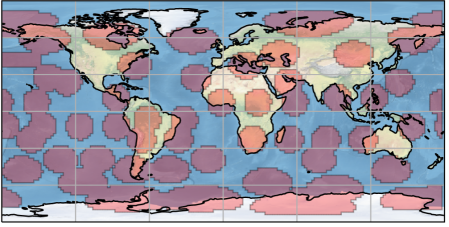
(a) Ground coverage obtained for $r_{i}=120$ and $CF=0.5$, time step $50$.

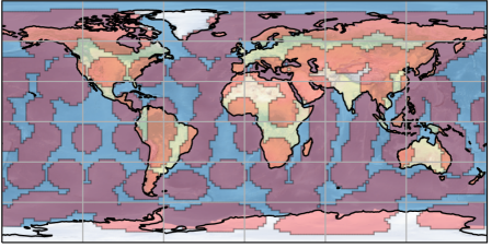
(b) Ground coverage obtained for $r_{i}=120$ and $CF=0.7$, time step $50$.

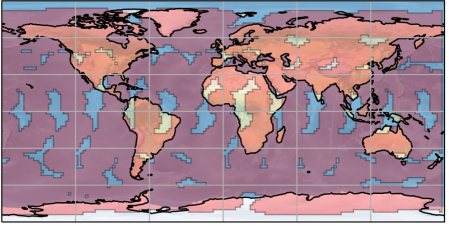
(c) Ground coverage obtained for $r_{i}=120$ and $CF=0.9$, time step $50$.

Fig. 4: Visualization of the ground coverage areas obtained at time step $50$ through DRG (Algorithm (2)) using $r_{i}=120$ and various $CF$.

6.2 Minimum Ground Coverage with DRG

We now consider a scenario where the goal of the decision-maker is to select a subset of satellites whose coverage area is at least a given fraction of the maximum achievable coverage area, which we denote by $CF$ while minimizing the incurred cost of the selection. This objective can naturally be expressed in terms of the performance-constrained optimization problem (9). For this simulation, we keep the same constellation parameters as in Subsection (6.1), with the exception of adjusting the inclination of the constellation to $75^{\mathrm{o}}$.

To calculate the area covered by a satellite, we first discretize Earth’s surface into a grid of cells of width and height $2^{\mathrm{o}}$. The area of each cell is then calculated assuming a spherical Earth. At each time step of the simulation, a cell’s area is said to be covered by a satellite if the centroid of that cell happens to be contained inside the field of view of a satellite. Straightforwardly, the marginal gain of including a satellite in the selection is the additional area that would be covered by that satellite, that is not already covered by the other satellites in the selection.

We test varying combinations of $r_{i}$ and $CF$ over a horizon of $100$ time steps, at each time step propagating the satellites in their orbit and subsequently running DRG to reconstruct a solution. Figure (4) displays visualizations for the resulting ground coverage obtained using a sampling set size of $r_{i}=120$, along with varying $CF$ values setting the coverage threshold. Tables (6.1) and (6.1) respectively display the average budget cost incurred and the average wall-clock computation time that DRG takes for each combination of $r_{i}$ and $CF$. We observe from the results that increasing the size of the sampling set in Algorithm (2) generally reduces the average cost of the satellite selection, but only marginally. However, it is clear from Table (6.1) that increasing the value of $r_{i}$ causes a significant increase in the wall-clock computation time needed for DRG to produce a solution. The results of both Subsections (6.1) and (6.2) demonstrate the benefit of incorporating randomization into the standard Greedy algorithm, as nearly identical costs for the selection budget can be achieved with a much lower computation time.

6.3 Multi-Objective Robustness with Random-WSSA

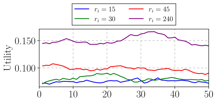
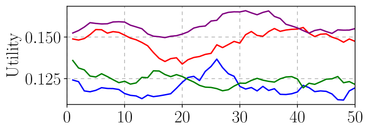
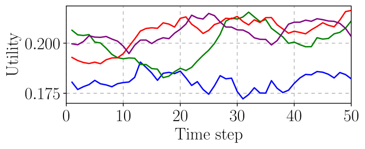
Fig. 5: Total utility over time for various $r_{i}$ and $B$ for the Random-WSSA. From top to bottom are the plots for $B=10$, $15$, and $20$, and $100$, respectively. The results are put through a moving average filter with a window size of $10$ for better visibility. Note that $r_{i}=240$ corresponds to using the entire ground set, i.e., the standard SSA.

Table 5: Average solution time in seconds for Random-WSSA for various $r_{i}$ and $B$. Note that $r_{i}=240$ corresponds to using the entire ground set, i.e., the standard SSA.

—c——c—c—c— $B=10$ $B=15$ $B=20$
$r_{i}=15$ $39.91$ $77.56$ $132.80$
$r_{i}=30$ $84.17$ $159.74$ $275.86$
$r_{i}=45$ $128.37$ $265.39$ $427.67$
$r_{i}=240$ $647.69$ $1559.20$ $2461.96$
Lastly, we move on to experimentally corroborating the results we obtain in Section (5). To reiterate, we deal with a notion of robustness that is ubiquitous in submodular optimization [44, 49, 50, 51], wherein we have multiple objectives aim to produce a solution that performs well with respect to all of them, subject to a budget constraint. We note that there are several other notions of robustness in the context of submodular optimization in the literature, one being robust to deletions. With this notion, the aim of the decision-maker is to construct solutions which, after the random removal of some of the elements they comprise, must adhere to a certain performance level. In real-world scenarios, this would be reflected by, for instance, being unable to connect to a selected satellite after the selection has been made. In the scope of this work, we are uninterested in this notion and proceed with the aforementioned notion.

We instantiate a constellation with the same parameters as in the previous subsection, tasked with accomplishing six distinct tasks. The first five tasks $f^{1},\ldots,f^{5}$ are atmospheric sensing tasks as in the experiments of Subsection (6.1). As opposed to that scenario, each task instantiates five randomly located points on Earth. The utility values $f^{1}(S),\ldots,f^{5}(S)$ of these tasks are proportionate to the additive inverse of the mean-squared error (MSE) achieved by the selection ${\mathcal{}S}$ of satellites.

The sixth task, $f^{6}$, involves ground coverage of the Earth. The utility value $f^{6}(S)$ of this task is proportionate to the Earth coverage achieved by the selected subset ${\mathcal{}S}$ of the satellites in the constellation. The area of coverage is determined based on the cell-grid structure explained in Subsection (6.2).

It is important to note that the utility of all six tasks $f^{1},\ldots,f^{6}$ is normalized to the range of $[0,1]$, by dividing the utility $f^{i}({\mathcal{}S})$ of a selection ${\mathcal{}S}$ on task $i$ at any time step by $f^{i}({\mathcal{}X})$, the maximum utility achievable by selecting the entire ground set at that time step. This ensures that the importance scores of individual tasks are not skewed by the arbitrary value of their utilities, and are solely dictated by the weight assigned to them.

We run the simulation for $50$ time steps and make robust selections using SSA and Random-WSSA with various random sampling set sizes. Figure (5) shows the comparison in terms of the utility achieved by the two algorithms, where the case of $r_{i}=240$ corresponds to the standard SSA, and $r_{i}=15$, $r_{i}=30$ and $r_{i}=45$ correspond to running Random-WSSA with various sampling set sizes. The results indicate that Random-WSSA achieves comparable performance to SSA as the size of the sampling set increases, especially in lower-budget settings. However, as is the case with the MRG algorithm, as the budget $B$ increases, we observe that the dependence on $r_{i}$ weakens, as the increase in budget allows for more room to retroactively correct suboptimal selections. It is also worth noting that both algorithms are run with $\alpha=1$, i.e., the non-relaxed version of the problem in terms of the budget constraint. Nevertheless, they are consistently able to produce solutions at each time step of the simulation.

Table (6.3) demonstrates the solution times for Random-WSSA for various combinations of $r_{i}$ and $B$. It is clear, in this case, that Random-WSSA enjoys significantly better computational complexity in comparison to SSA, taking nearly twenty times as less time as SSA in some cases, whereas SSA takes longer than $10$ minutes on average for a single iteration even in the low-budget scenario of $B=10$. It is straightforward to conclude, then, that SSA is infeasible in time-critical conditions and that our proposed Random-WSSA is much better-suited to such scenarios.

7 Conclusion

We introduced three novel algorithms, namely the Modified Randomized Greedy, the Dual Randomized Greedy, and Randomized Weak Submodular Saturation Algorithm. The first two of these algorithms aim to address weak submodular maximization problems under budget and performance constraints, respectively. The last aims to achieve multi-objective robustness in the presence of performance constraints. Subsequently, we provided theoretical guarantees that hold with high probability on the performance of these algorithms. We illustrated the efficacy of the three algorithms through a practical scenario involving a sensors selection problem, where the sensors in question are satellites in a LEO constellation.

A clear avenue for potential research is the further investigation of the martingale assumption. One could explore whether domain-specific knowledge can enhance the tightness of the obtained bounds, or whether a guarantee that holds on expectation for the Dual Randomized Greedy could be established, with the aim of using it in conjunction with a post-optimization-based method using multiple parallel instances of the algorithm to obtain a guarantee that holds with high probability.

8 Acknowledgments

This work is supported in part by DARPA grant HR00112220025.

References

- [1] M. G. Damavandi, V. Krishnamurthy, and J. R. Martí, “Robust meter placement for state estimation in active distribution systems,” IEEE Transactions on Smart Grid, vol. 6, no. 4, pp. 1972–1982, 2015.
- [2] Z. Liu, A. Clark, P. Lee, L. Bushnell, D. Kirschen, and R. Poovendran, “Towards scalable voltage control in smart grid: a submodular optimization approach,” in Proceedings of the 7th International Conference on Cyber-Physical Systems, p. 20, IEEE Press, 2016.
- [3] N. Buchbinder, M. Feldman, J. S. Naor, and R. Schwartz, “Submodular maximization with cardinality constraints,” in Proceedings of the Twenty-Fifth Annual ACM-SIAM Symposium on Discrete Algorithms, SODA ’14, (USA), p. 1433–1452, Society for Industrial and Applied Mathematics, 2014.
- [4] S. Dughmi, T. Roughgarden, and M. Sundararajan, “Revenue submodularity,” in Auctions, Market Mechanisms and Their Applications (S. Das, M. Ostrovsky, D. Pennock, and B. Szymanksi, eds.), (Berlin, Heidelberg), pp. 89–91, Springer Berlin Heidelberg, 2009.
- [5] A. S. Schulz and N. A. Uhan, “Approximating the least core value and least core of cooperative games with supermodular costs,” Discrete Optimization, vol. 10, no. 2, pp. 163–180, 2013.
- [6] G. Attigeri, M. Manohara Pai, and R. M. Pai, “Feature selection using submodular approach for financial big data,” Journal of Information Processing Systems, vol. 15, no. 6, pp. 1306–1325, 2019.
- [7] R. A. Richards, R. T. Houlette, J. L. Mohammed, et al., “Distributed satellite constellation planning and scheduling.,” in FLAIRS Conference, pp. 68–72, 2001.
- [8] D. P. Williamson and D. B. Shmoys, The design of approximation algorithms. Cambridge university press, 2011.
- [9] G. L. Nemhauser, L. A. Wolsey, and M. L. Fisher, “An analysis of approximations for maximizing submodular set functions,” Mathematical Programming, vol. 14, no. 1, pp. 265–294, 1978.
- [10] L. A. Wolsey, “An analysis of the greedy algorithm for the submodular set covering problem,” Combinatorica, vol. 2, no. 4, pp. 385–393, 1982.
- [11] S. Khuller, A. Moss, and J. S. Naor, “The budgeted maximum coverage problem,” Information processing letters, vol. 70, no. 1, pp. 39–45, 1999.
- [12] B. Mirzasoleiman, A. Badanidiyuru, A. Karbasi, J. Vondrak, and A. Krause, “Lazier than lazy greedy,” in AAAI Conference on Artificial Intelligence, AAAI, 2015.
- [13] A. Hashemi, M. Ghasemi, H. Vikalo, and U. Topcu, “Randomized greedy sensor selection: Leveraging weak submodularity,” IEEE Transactions on Automatic Control, vol. 66, no. 1, pp. 199–212, 2021.
- [14] A. Krause and D. Golovin, “Submodular function maximization,” in Tractability: Practical Approaches to Hard Problems, pp. 71–104, Cambridge University Press, 2014.
- [15] M. Hibbard, A. Hashemi, T. Tanaka, and U. Topcu, “Randomized greedy algorithms for sensor selection in large-scale satellite constellations,” Proceedings of the American Control Conference, 2023.
- [16] A. Poghosyan and A. Golkar, “CubeSat evolution: Analyzing CubeSat capabilities for conducting science missions,” Progress in Aerospace Sciences, vol. 88, pp. 59–83, 2017.
- [17] K. M. Wagner, K. K. Schroeder, and J. T. Black, “Distributed space missions applied to sea surface height monitoring,” Acta Astronautica, vol. 178, pp. 634–644, 2021.
- [18] K. Cahoy and A. K. Kennedy, “Initial results from ACCESS: an autonomous CubeSat constellation scheduling system for Earth observation,” 2017.
- [19] W. J. Blackwell, S. Braun, R. Bennartz, C. Velden, M. DeMaria, R. Atlas, J. Dunion, F. Marks, R. Rogers, B. Annane, et al., “An overview of the TROPICS NASA Earth venture mission,” Quarterly Journal of the Royal Meteorological Society, vol. 144, pp. 16–26, 2018.
- [20] C. Boshuizen, J. Mason, P. Klupar, and S. Spanhake, “Results from the planet labs flock constellation,” 2014.
- [21] D. Selva and D. Krejci, “A survey and assessment of the capabilities of CubeSats for Earth observation,” Acta Astronautica, vol. 74, pp. 50–68, 2012.
- [22] D. Mandl, G. Crum, V. Ly, M. Handy, K. F. Huemmrich, L. Ong, B. Holt, and R. Maharaja, “Hyperspectral CubeSat constellation for natural hazard response,” in Annual AIAA/USU Conference on Small Satellites, no. GSFC-E-DAA-TN33317, 2016.
- [23] G. Santilli, C. Vendittozzi, C. Cappelletti, S. Battistini, and P. Gessini, “CubeSat constellations for disaster management in remote areas,” Acta Astronautica, vol. 145, pp. 11–17, 2018.
- [24] S. Nag, J. L. Rios, D. Gerhardt, and C. Pham, “CubeSat constellation design for air traffic monitoring,” Acta Astronautica, vol. 128, pp. 180–193, 2016.
- [25] S. Wu, W. Chen, C. Cao, C. Zhang, and Z. Mu, “A multiple-CubeSat constellation for integrated earth observation and marine/air traffic monitoring,” Advances in Space Research, vol. 67, no. 11, pp. 3712–3724, 2021.
- [26] S. Siewert and L. McClure, “A system architecture to advance small satellite mission operations autonomy,” 1995.
- [27] A. Hashemi, M. Ghasemi, H. Vikalo, and U. Topcu, “A randomized greedy algorithm for near-optimal sensor scheduling in large-scale sensor networks,” in American Control Conference (ACC), pp. 1027–1032, IEEE, 2018.
- [28] U. Feige, “A threshold of ln n for approximating set cover,” Journal of the ACM, vol. 45, no. 4, pp. 634–652, Jul. 1998.
- [29] H. Zhang and Y. Vorobeychik, “Submodular optimization with routing constraints,” in AAAI Conference on Artificial Intelligence, 2016.
- [30] L. Chamon and A. Ribeiro, “Approximate supermodularity bounds for experimental design,” in Advances in Neural Information Processing Systems (NIPS), pp. 5409–5418, 2017.
- [31] A. Hashemi, M. Ghasemi, and H. Vikalo, “Submodular observation selection and information gathering for quadratic models,” in Proceedings of the 36th International Conference on Machine Learning, vol. 97, 2019.
- [32] A. Das and D. Kempe, “Submodular meets spectral: Greedy algorithms for subset selection, sparse approximation and dictionary selection,” in Proceedings of the International Conference on Machine Learning (ICML), pp. 1057–1064, 2011.
- [33] E. R. Elenberg, R. Khanna, A. G. Dimakis, and S. Negahban, “Restricted strong convexity implies weak submodularity,” The Annals of Statistics, vol. 46, no. 6B, pp. 3539–3568, 2018.
- [34] T. Horel and Y. Singer, “Maximization of approximately submodular functions,” in Advances in Neural Information Processing Systems (NIPS), pp. 3045–3053, 2016.
- [35] A. A. Bian, J. M. Buhmann, A. Krause, and S. Tschiatschek, “Guarantees for greedy maximization of non-submodular functions with applications,” in International Conference on Machine Learning (ICML), pp. 498–507, Omnipress, 2017.
- [36] R. Khanna, E. Elenberg, A. Dimakis, S. Negahban, and J. Ghosh, “Scalable greedy feature selection via weak submodularity,” in Artificial Intelligence and Statistics, pp. 1560–1568, 2017.
- [37] M. Ghasemi, A. Hashemi, U. Topcu, and H. Vikalo, “On submodularity of quadratic observation selection in constrained networked sensing systems,” in 2019 American Control Conference (ACC), pp. 4671–4676, IEEE, 2019.
- [38] A. Hashemi, H. Vikalo, and G. de Veciana, “On the performance-complexity tradeoff in stochastic greedy weak submodular optimization,” in ICASSP 2021-2021 IEEE International Conference on Acoustics, Speech and Signal Processing (ICASSP), pp. 3540–3544, IEEE, 2021.
- [39] A. Hashemi, H. Vikalo, and G. de Veciana, “On the benefits of progressively increasing sampling sizes in stochastic greedy weak submodular maximization,” IEEE Transactions on Signal Processing, vol. 70, pp. 3978–3992, 2022.
- [40] A. Hassidim and Y. Singer, “Robust guarantees of stochastic greedy algorithms,” in International Conference on Machine Learning, pp. 1424–1432, PMLR, 2017.
- [41] F. Chung and L. Lu, “Concentration inequalities and martingale inequalities: a survey,” Internet Mathematics, vol. 3, no. 1, pp. 79–127, 2006.
- [42] K. D. Harris, “The martingale z-test,” 2022.
- [43] A. Das and D. Kempe, “Approximate submodularity and its applications: Subset selection, sparse approximation and dictionary selection,” Journal of Machine Learning Research, vol. 19, no. 3, pp. 1–34, 2018.
- [44] A. Krause, H. B. McMahan, C. Guestrin, and A. Gupta, “Robust submodular observation selection,” Journal of Machine Learning Research, vol. 9, no. 93, pp. 2761–2801, 2008.
- [45] L. A. Wolsey, “An analysis of the greedy algorithm for the submodular set covering problem,” Combinatorica, vol. 2, no. 4, pp. 385–393, 1982.
- [46] J. G. Walker, “Satellite constellations,” Journal of the British Interplanetary Society, vol. 37, p. 559, 1984.
- [47] E. N. Lorenz, “Deterministic nonperiodic flow,” Journal of atmospheric sciences, vol. 20, no. 2, pp. 130–141, 1963.
- [48] Y. Bar-Shalom, X. R. Li, and T. Kirubarajan, Estimation with applications to tracking and navigation: theory algorithms and software. John Wiley & Sons, 2004.
- [49] A. Ben-Tal, L. El Ghaoui, and A. Nemirovski, Robust optimization, vol. 28. Princeton university press, 2009.
- [50] A. Ben-Tal and A. Nemirovski, “Robust optimization–methodology and applications,” Mathematical programming, vol. 92, pp. 453–480, 2002.
- [51] R. Udwani, “Multi-objective maximization of monotone submodular functions with cardinality constraint,” in Advances in Neural Information Processing Systems (S. Bengio, H. Wallach, H. Larochelle, K. Grauman, N. Cesa-Bianchi, and R. Garnett, eds.), vol. 31, Curran Associates, Inc., 2018.