vl short = VL , long = vision-language \DeclareAcronymkyn short = KYN , long = Know Your Neighbors \DeclareAcronymvlm short = VLM , long = vision-language modulation \DeclareAcronymvlsa short = VLSA , long = vision-language spatial attention
Know Your Neighbors: Improving Single-View Reconstruction
via Spatial Vision-Language Reasoning
Abstract
Recovering the 3D scene geometry from a single view is a fundamental yet ill-posed problem in computer vision. While classical depth estimation methods infer only a 2.5D scene representation limited to the image plane, recent approaches based on radiance fields reconstruct a full 3D representation. However, these methods still struggle with occluded regions since inferring geometry without visual observation requires (i) semantic knowledge of the surroundings, and (ii) reasoning about spatial context. We propose KYN, a novel method for single-view scene reconstruction that reasons about semantic and spatial context to predict each point’s density. We introduce a vision-language modulation module to enrich point features with fine-grained semantic information. We aggregate point representations across the scene through a language-guided spatial attention mechanism to yield per-point density predictions aware of the 3D semantic context. We show that KYN improves 3D shape recovery compared to predicting density for each 3D point in isolation. We achieve state-of-the-art results in scene and object reconstruction on KITTI-360, and show improved zero-shot generalization compared to prior work. Project page: https://ruili3.github.io/kyn.
1 Introduction
Humans have the extraordinary ability to estimate the geometry of a 3D scene from a single image, often including its occluded parts. It enables us to reason about where dynamic actors in the scene might move, and how to best navigate ourselves to avoid a collision. Hence, estimating the 3D scene geometry from a single input view is a long-standing challenge in computer vision, fundamental to autonomous navigation [16] and virtual reality applications [33]. Since the problem is highly ill-posed due to scale ambiguity, occlusions, and perspective distortion, it has traditionally been cast as a 2.5D problem [58, 31, 6], focusing on areas visible in the image plane and neglecting the non-visible parts.
Recently, approaches based on neural radiance fields [39] have shown great potential in inferring the true 3D scene representation from a single [59, 51] or multiple views [50]. For instance, Wimbauer et al. [51] introduce BTS, a method that estimates a 3D density field from a single view at inference while being supervised only by photometric consistency given multiple posed views at training time.
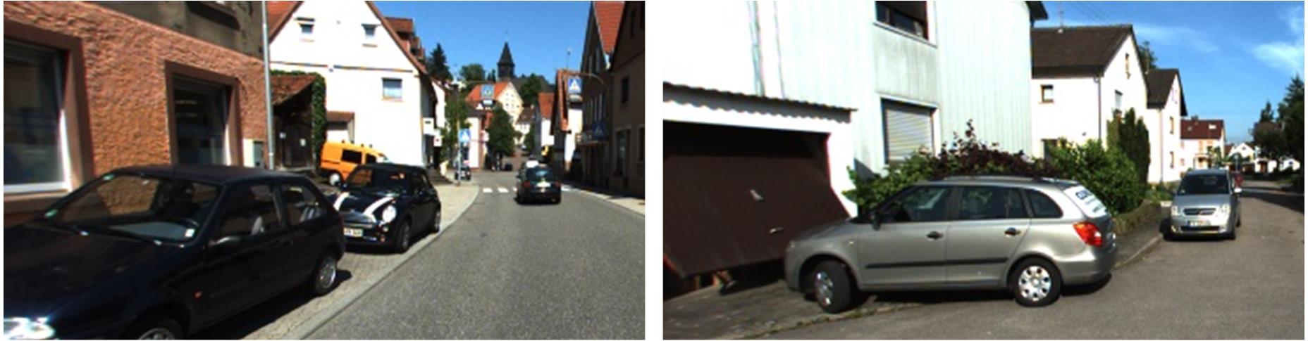
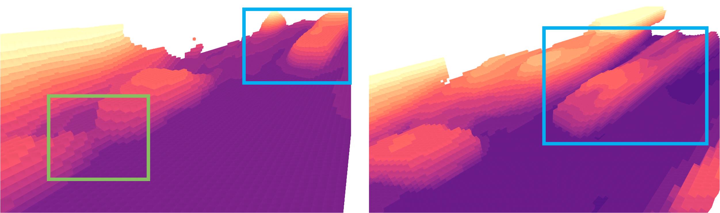
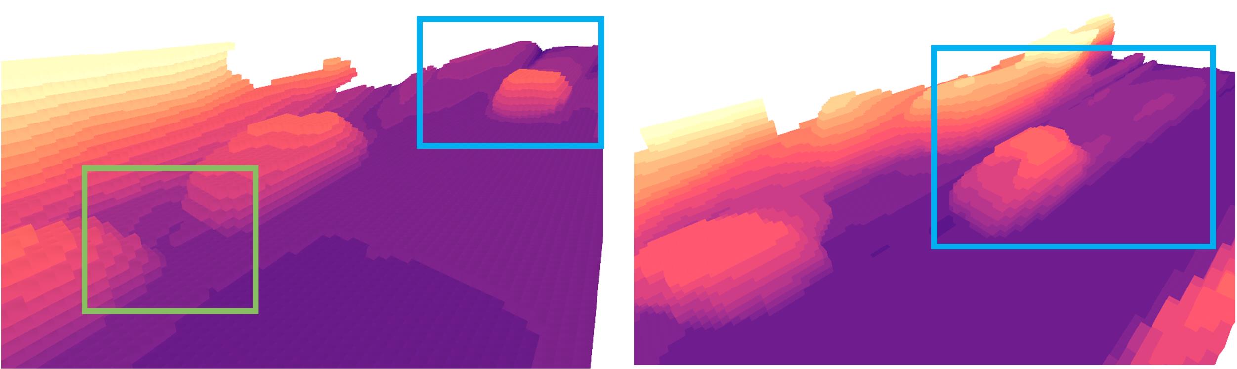
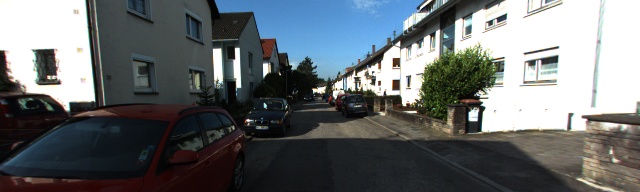
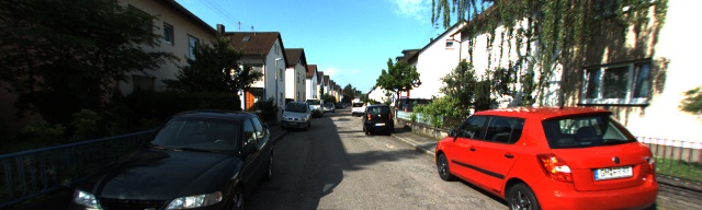
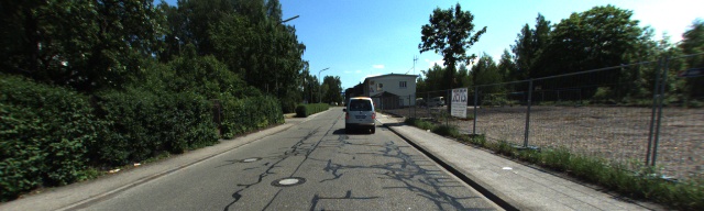
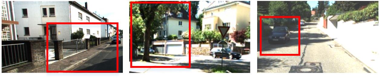
Intuitively, given only a single image at inference, the model must rely on semantic knowledge from the neighboring 3D structure to predict the density of occluded points. However, existing approaches lack explicit semantic modeling and, by modeling density prediction independently for each point, are unaware of the semantic 3D context of the point’s surroundings. This results in the clear limitations which we illustrate in Fig. 1. Specifically, prior work [51] struggles with accurate shape recovery (green) and further exhibits trailing effects (blue) in the absence of visual observation. We argue that, when considering a single point in 3D, its density highly depends on the semantic scene context, e.g. if there is an intersection, a parking lot, or a sidewalk visible in its proximity. This becomes more critical as we move further from the camera origin since the degree of visual coverage decreases with distance, and reconstructing the increasingly unobserved scene parts requires context from the neighboring points.
To this end, we present \ackyn, a novel approach for single-view scene reconstruction that predicts density for each 3D point in a scene by reasoning about its neighboring semantic and spatial context. We introduce two key innovations. We develop a \acvl modulation scheme that endows the representation of each 3D point in space with fine-grained semantic information. To leverage this information, we further introduce a \acvl spatial attention mechanism that utilizes language guidance to aggregate the visual semantic point representations across the scene and predict the density of each individual point as a function of the neighboring semantic context.
We show that, by injecting semantic knowledge and reasoning about spatial context, our method overcomes the limitations that prior art exhibits in unobserved areas, producing more plausible 3D shapes and mitigating their trailing effects. We summarize our contributions as follows:
-
•
We propose \ackyn, the first single-view scene reconstruction method that reasons about semantic and spatial context to predict each point’s density.
-
•
We introduce a \acvl modulation module to enrich point features with fine-grained semantic information.
-
•
We propose a \acvl spatial attention mechanism that aggregates point representations across the scene to yield per-point density predictions aware of the neighboring 3D semantic context.
Our experiments on the KITTI-360 dataset [34] show that \ackyn achieves state-of-the-art scene and object reconstructions. Furthermore, we demonstrate that \ackyn exhibits better zero-shot generalization on the DDAD dataset [18] compared to the prior art.
2 Related Work
Monocular depth estimation. Estimating depth from a single view has been extensively studied over the last decade [55, 58, 57, 56, 36, 35], both in a supervised and a self-supervised manner. Supervised methods directly minimize the loss between the predicted and ground truth depths [11, 1]. For these, varying output representations [14, 1, 2], network architectures [1, 61, 43, 27], and loss functions [1, 52, 48] have been proposed. Recent methods explore training unified depth models on large datasets, tackling challenges like varying camera intrinsics [42, 56, 58, 12, 20] and dataset bias [3]. Self-supervised methods cast the problem as a view synthesis task and learn depth via photometric consistency on image pairs. Existing works have investigated how to handle dynamic objects [31, 17, 13, 30, 46, 7], different network architectures [64, 62, 37, 53] and leveraging additional constraints [19, 32, 47, 44]. Our method falls in the self-supervised category. However, we estimate a true 3D representation from a single view, as opposed to the 2.5D representation produced by traditional depth estimation.
Semantic priors for depth estimation. Previous depth estimation methods use semantic information to enhance 2D feature representations with different fusion strategies [19, 22, 32, 8], or to remove dynamic objects [5, 28] during training. These methods utilize semantic information in the 2D representation space. On the contrary, we use semantic information to enhance 3D point representations and to guide our 3D spatial attention mechanism.
Neural radiance fields. Neural radiance fields (NeRFs) [39, 59] learn a volumetric 3D representation of the scene from a set of posed input views. In particular, they use volumetric rendering in order to synthesize novel views by sampling volume density and color along a pixel ray. Recent multi-view reconstruction methods [49, 54, 60] take inspiration from this paradigm, reformulating the volume density function as a signed distance function for better surface reconstruction. These methods are focused on single-scene optimization using multi-view constraints, often representing the scene with the weights of a single MLP.
To address the issue of generalization across scenes, Yu et al. [59] propose PixelNeRF to train a CNN image encoder across scenes that is used to condition an MLP, predicting volume density and color without multi-view optimization during inference. However, their approach is limited to small-scale and synthetic datasets. Recently, Wimbauer et al. [51] proposed BTS, an extension of PixelNeRF to large-scale outdoor scenes. They omit the color prediction and, during training, use reference images to query color for a 3D point given a density field that represents the 3D scene geometry. While this simplification allows them to scale to large-scale outdoor scenes, their method falls short in predicting accurate geometry for occluded areas (Fig. 1). We address this shortcoming by injecting fine-grained semantic knowledge and reasoning about semantic 3D context when querying the density field, leading to better shape recovery for occluded regions in particular.
Scene as occupancy. A recent line of work infers 3D scene geometry as voxelized 3D occupancy [4, 38] from a single image. These works predict the occupancy and semantic class of each 3D voxel based on exhaustive 3D annotations. Therefore, these methods rely heavily on manually annotated datasets. Further, the predefined voxel resolution limits the fidelity of their 3D representation. In contrast, our method does not rely on labor-intensive manual annotations and represents the scene as a continuous density field.
Semantic priors for NeRFs. Various works integrate semantic priors into NeRFs. While some utilize 2D semantic or panoptic semgentation [63, 15, 26], others leverage 2D \acvl features [24, 13, 41] and lift these into 3D space by distilling them into the NeRF. This enables the generation of 2D segmentation masks from new viewpoints, segmenting objects in 3D space, and discovering or removing particular objects from a 3D scene. While the aforementioned methods focus on the classical multi-view optimization setting, we instead focus on single-view input and leverage semantic priors to improve the 3D representation itself.
3 Method
Problem setup. Given an input image , its corresponding intrinsics and pose , we aim to reconstruct the full 3D scene by estimating the density for each 3D point among point set
| (1) |
where the density of point is a function of the point set and image along with its camera intrinsic/extrinsics. denotes the network and represents its parameters. The density can be further transformed to the binary occupancy score with a predefined threshold . During training (Sec. 3.3), additional images are incorporated with their corresponding intrinsics and extrinsics , with , providing multiview supervision.
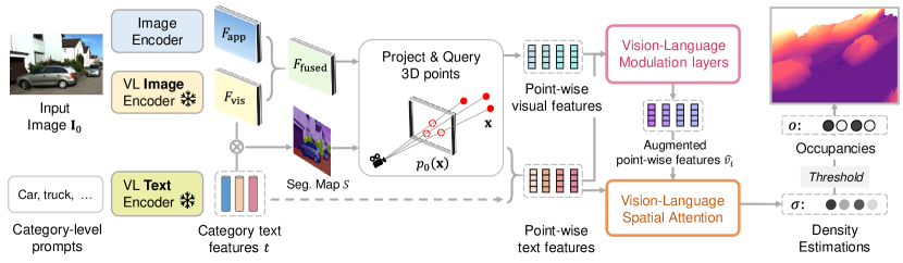
Overview. We illustrate our method in Fig. 2. Given an input image , we first extract image and \acvl feature maps and . Next, we fuse the image and \acvl features into a single feature map and further utilize category-wise text features to compute a segmentation map . We then use intrinsics to project the 3D point set to the image plane and query , yielding point-wise visual features. In parallel, we retrieve point-wise text features by querying the segmentation map and looking up the corresponding category-wise text features for each 3D point. Given the point-wise visual and text features, we use our \acvl modulation layers to augment the features with fine-grained semantic information. We aggregate the point-wise features with \acvl spatial attention, adding 3D semantic context to the point-wise features. We guide the attention mechanism with the \acvl text features. We finally predict a per-point density that is thresholded to yield the 3D occupancy map.
3.1 Vision-Lanugage Modulation
We detail how we extract point-wise visual features and how we augment the visual features with semantic information using our \acvl modulation module.
Point-wise visual feature extraction. Given the input image , we extract image features from standard image encoders [21] and \acvl image encoder [29]
| (2) | ||||
where and refer to the appearance features and \acvl image features, respectively. We freeze the \acvl image encoder weights to retain the pre-trained semantics. We then fuse the features by concatenation followed by 2 convolutional layers, yielding . To obtain point-wise features for the 3D points , we extract the fused feature w.r.t. the projected 2D coordinates of each 3D point. Then, we combine each 3D point feature with a positional embedding encoding its position in normalized device coordinates (NDC). We obtain the fused point-wise visual feature for a 3D point
| (3) |
where is the feature concatenation operation, and is the 3D position w.r.t. ’s coordinate.
Point-wise text feature extraction. As the text feature size does not align with the image space, it can not be extracted directly by querying projected 2D coordinates. To this end, we first derive the semantic category of each 3D point through 2D segmentations. Then we use it to associate text features with each 3D point. We utilize the category names from outdoor scenes [9] as prompts to the text encoder, yielding the text features , where is the number of categories and is the feature channel. We then use the visual feature from the \acvl image encoder, to obtain the 2D semantic map by computing cosine similarity between \acvl image and text features
| (4) |
where denotes matrix multiplication, denotes the segmentation map by maximizing the similarity scores between \acvl image and text features along the category dimension. We then compute the semantic category for each 3D point by querying with projected 2D coordinates and then leverage it to obtain the text feature of each 3D point.
| (5) | ||||
where is the text feature of the 3D point .
vl modulation layers. To augment the 3D point features with rich semantics from both \acvl image and text features, we propose the \acvl modulation layers, which integrate both image feature and text representations of a 3D point for better scene geometry reasoning. The module is composed of modulation layers, each conducting modulation with multiplication operations
| (6) |
where stands for the fully connected layer, is the element-wise product between features, denotes the text features encoded by a single fully-connected layer and is shared across different modulation layers. We set at the first modulation layer, and iterate through different layers. We utilize skip connections to inject the initial visual information after the modulated feature at level , using concatenation followed by one fully-connected layer. The output feature denotes the 3D point feature of augmented with rich image and text semantics.
3.2 \acvl Spatial Attention
Next, we dive into our \acvl spatial attention mechanism that aggregates the extracted point-wise features across the scene in a global-to-local fashion. First, we combine the whole set of point-wise visual features and text features into and . Then, we aggregate these features using a cross-attention operation in 3D space. Specifically, we leverage linear attention [23, 45] over appropriately split point sets to achieve memory-efficient spatial context reasoning.
Category-informed cross-attention. We take the point-wise features as queries and values, and leverage text-based feature as the keys in the linear attention. Specifically, we project the features with fully connected layers to keys, queries, and values
| (7) | ||||
where all features are in , where denotes the feature dimension before the attention. We then compute the global context score by attending to the key and value features, and then correlating with query features by
| (8) | ||||
where denotes the spatially aggregated point-wise features. The density value is estimated by a single fully connected layer followed by a Softplus function
| (9) |
Reducing the memory footprint. As the point features are sampled from the entire 3D space, simultaneously processing all point features can hit computational bottlenecks even with linear attention. To this end, we randomly split the initial points into chunks, to ensure that each chunk is identically distributed. Then we conduct the spatial point attention separately within each chunk and combine the density estimations afterward. As such, the attention can aggregate semantic point representations with both spatial awareness and efficiency.
Input
Ours
3.3 Training Process
Our method achieves self-supervision by computing the photometric loss between the reconstructed and target colors. We extract the 2D feature map of to get point-wise representations, then partition all images into a source set and a loss set following previous practice [51]. We render the RGB of from the corresponding colors of similar to the self-supervised depth estimation [17]. Instead of resorting to the whole image, we perform patch-based image supervision [51] to reduce memory footprints. For each pixel on a patch, we sample the 3D points on its back-projected ray and conduct density estimation. Let and be the adjacent sampled pixels on a ray, we calculate the RGB information by volume rendering the sampled color [51]
| (10) |
| (11) |
where denotes the distance between adjacent sampled points and along the ray, and refer to the probability that the ray ends between and . Note that the color is the sampled RGB value from the view in the source set , to obtain a better geometry. and represent the terminating depth and the rendered color.
As we sample the pixels in a patch-wise manner during training, the rendered RGB and depth are also organized in patches. Let as the rendered patch from view in the source , as the supervisory patch from , and as the patch depth of , the loss function is defined following previous methods [51, 17]
| (12) |
where , and are photometric loss and edge-aware smoothness loss [17] on patches
| (13) |
| (14) |
where and , denotes the gradient along the horizontal and vertical directions.
4 Experiments
To demonstrate the effectiveness of our proposed method, we compare with existing works [62, 17, 59, 51] in single-view scene reconstruction, including both depth estimation [17] and radiance field based methods [59, 51]. We evaluate both the 3D scene (Sec. 4.4) and object (Sec. 4.5) reconstruction results on the KITTI-360 dataset in short and long ranges. We conduct extensive ablations (Sec. 4.6) to verify the effectiveness of each contribution, compare our method with existing semantic feature fusion techniques, as well as evaluate our method’s performance with the broader supervision range. Moreover, we demonstrate our method’s zero-shot generalization ability in Sec. 4.7.
4.1 Datasets
We use the KITTI-360 [34] dataset for training and evaluation, as it captures static scenes using cameras deployed with wide baselines, i.e., two stereo cameras, and two side cameras (fisheye cameras) at each timestep, which facilitate learning full 3D shapes by self-supervision. During the training phase, we use all cameras from two time steps, i.e. 8 cameras in total, to train our model. We use an input resolution of 192640 and choose the left stereo camera from the first time step to extract the image features. We split all cameras randomly into and for sampling colors and loss computation, as is illustrated in Sec. 3.3. Furthermore, we use the DDAD [18] dataset to evaluate the zero-shot generalization capability of the models trained on KITTI-360. We select testing sequences with more than 50 images and use 384640 image resolution.
| Method | O | IE | IE | |
|---|---|---|---|---|
| 4-20m | Monodepth2 [17] | 0.90 | n/a | n/a |
| Monodepth2 [17] + | 0.90 | 0.59 | 0.66 | |
| PixelNeRF [59] | 0.89 | 0.62 | 0.60 | |
| BTS [51] | 0.92 | 0.66 | 0.64 | |
| Ours | 0.92 | 0.70 | 0.72 | |
| 4-50m | Monodepth2 [17] | 0.82 | n/a | n/a |
| Monodepth2 [17] + | 0.81 | 0.54 | 0.76 | |
| PixelNeRF [59] | 0.82 | 0.56 | 0.68 | |
| BTS [51] | 0.84 | 0.61 | 0.53 | |
| Ours | 0.86 | 0.63 | 0.73 | |
4.2 Evaluation
We follow the experimental protocol in [51] to evaluate 3D occupancy prediction. Specifically, we sample 3D grid points on 2D slices parallel to the ground plane. For KITTI-360, we report scores within distance ranges and meters, where the latter provides a more challenging evaluation scenario. For ground-truth generation, we follow [51] and accumulate 3D LiDAR points across time, and set 3D points lying out of all depth surfaces as unoccupied, otherwise set to occupied. Unlike [51], which accumulate only 20 LiDAR sweeps often leading to inaccurate occluded scene geometry, we accumulate up to 300 LiDAR frames. We also provide results with a 20-frame accumulated ground truth in the supplementary material for reference. For the DDAD dataset, we accumulate up to 100 LiDAR frames due to the limited sequence length and evaluate in the meters range.
Metrics. We adopt the evaluation metrics in [51] and measure overall reconstruction (O) and occluded reconstruction (IE, IE) accuracies. Specifically, O computes the accuracy between the prediction and the ground truth in the full area of the evaluation range, thus reflecting the overall performance of the reconstruction. IE computes the accuracy of the invisible areas specifically, i.e. without direct visual observation in . IE computes the recall of both invisible and empty areas, which evaluates the reconstruction of the occluded empty space. The three metrics focus on different aspects of the reconstruction quality.
Scene- and object-level evaluation. In addition to evaluating the performance of the whole scene, we focus on object reconstruction in particular because they are of particular interest compared to e.g. the road plane. To this end, we manually annotate the object areas in the ground-truth occupancy maps and compute the evaluation metrics on these object areas. We refer the reader to the supplementary material for details.
4.3 Implementation Details
We implement our method using Pytorch [40] and train it on NVIDIA Quadro RTX 6000 GPUs. The appearance network is similar to [17] with pre-trained weights on ImageNet [10]. We adopt LSeg [29] as the visual-language network and freeze its parameters. The model is trained using Adam [25] optimizer with a learning rate of for 25 epochs, which is reduced to after 120k iterations. During the training phase, we sample 4096 patches across loss set , each patch contains pixels. We further sample 64 points along each ray following [51].
4.4 Scene Reconstruction
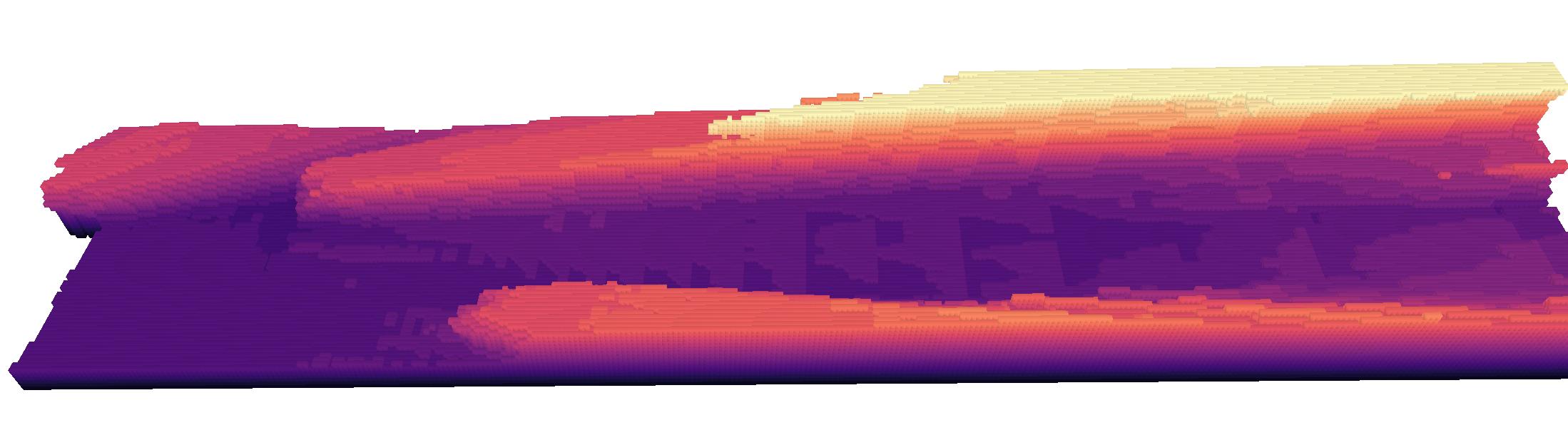
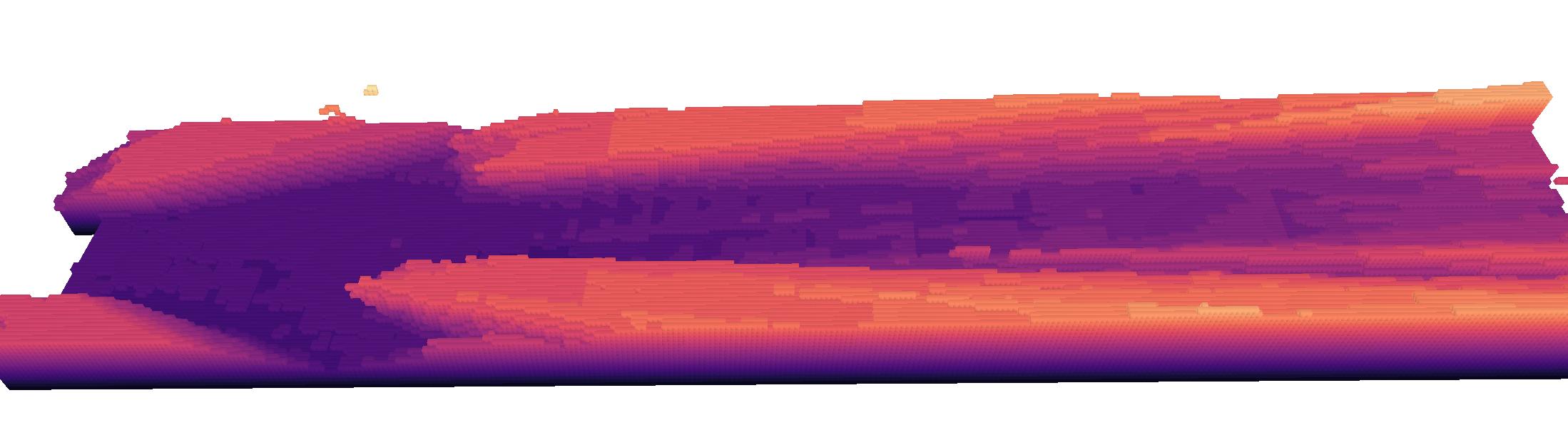
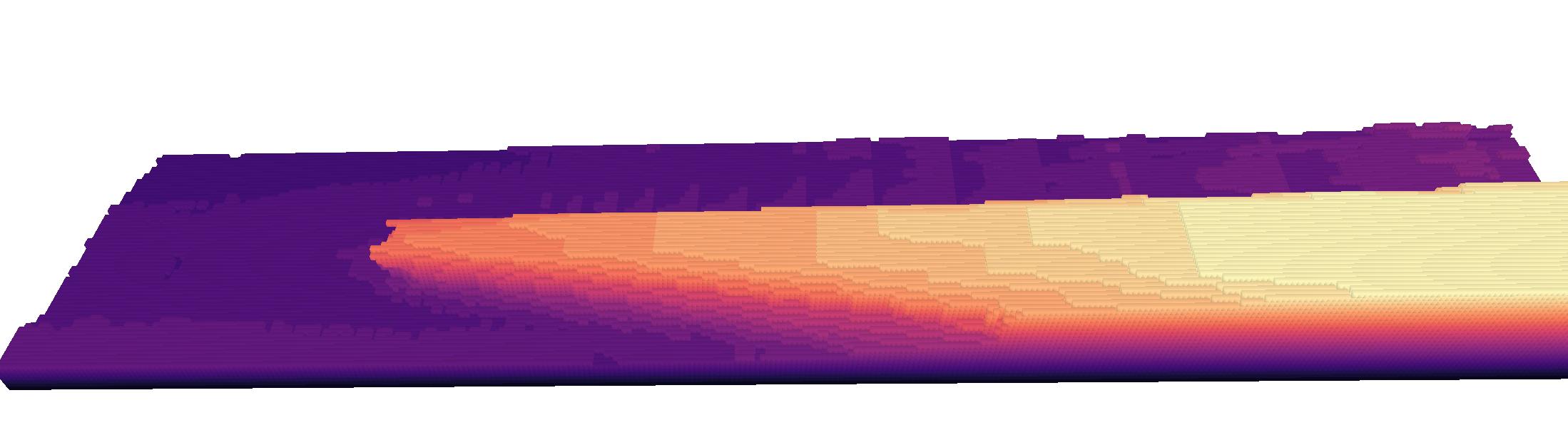
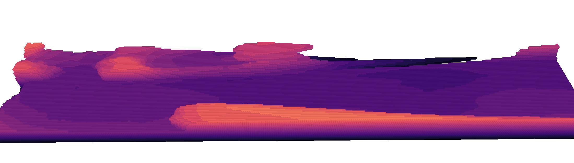
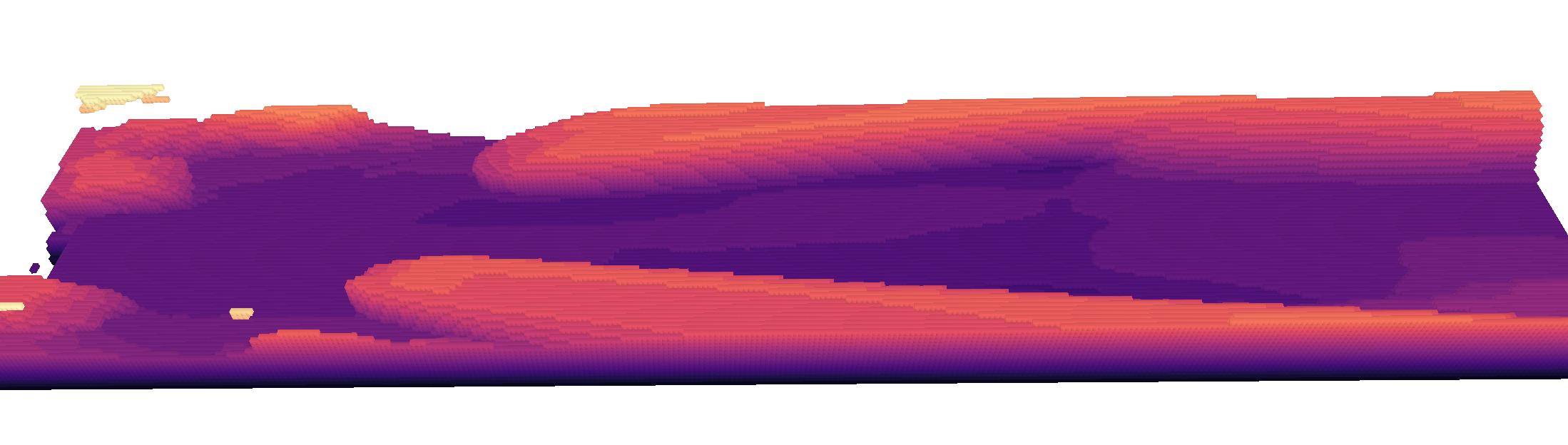
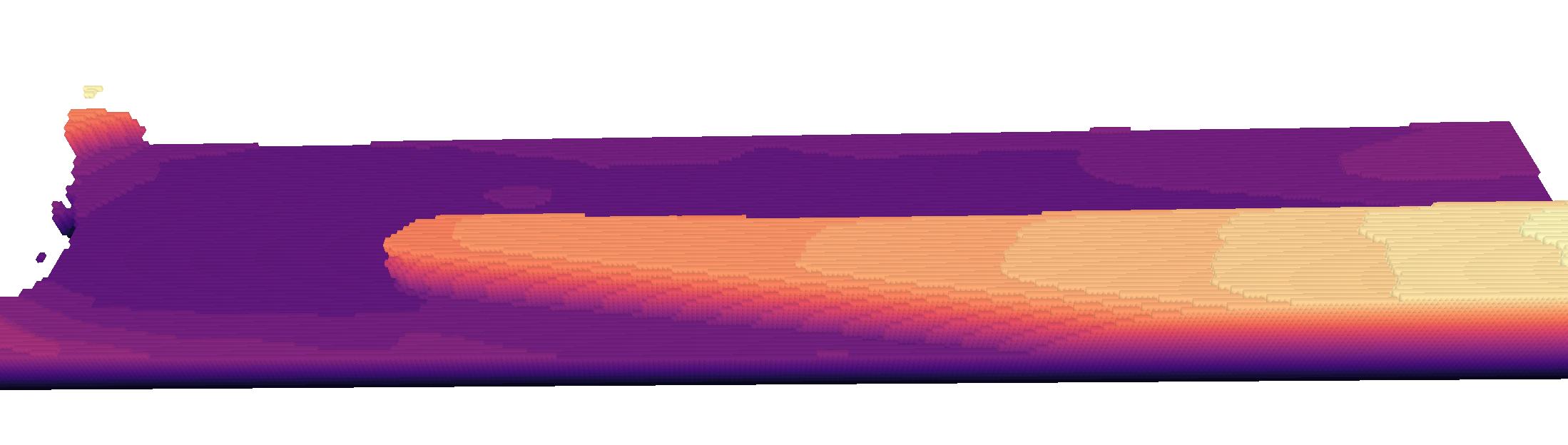
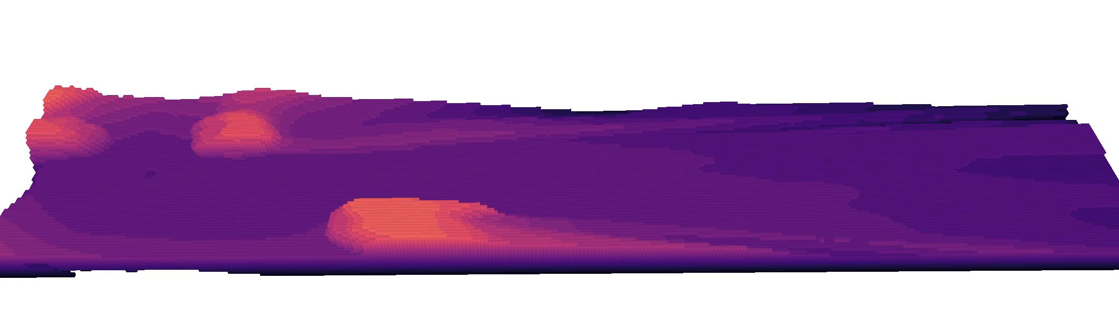
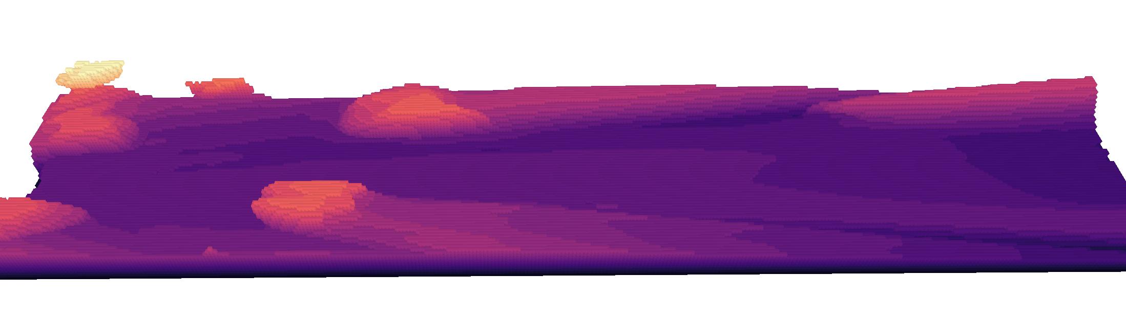
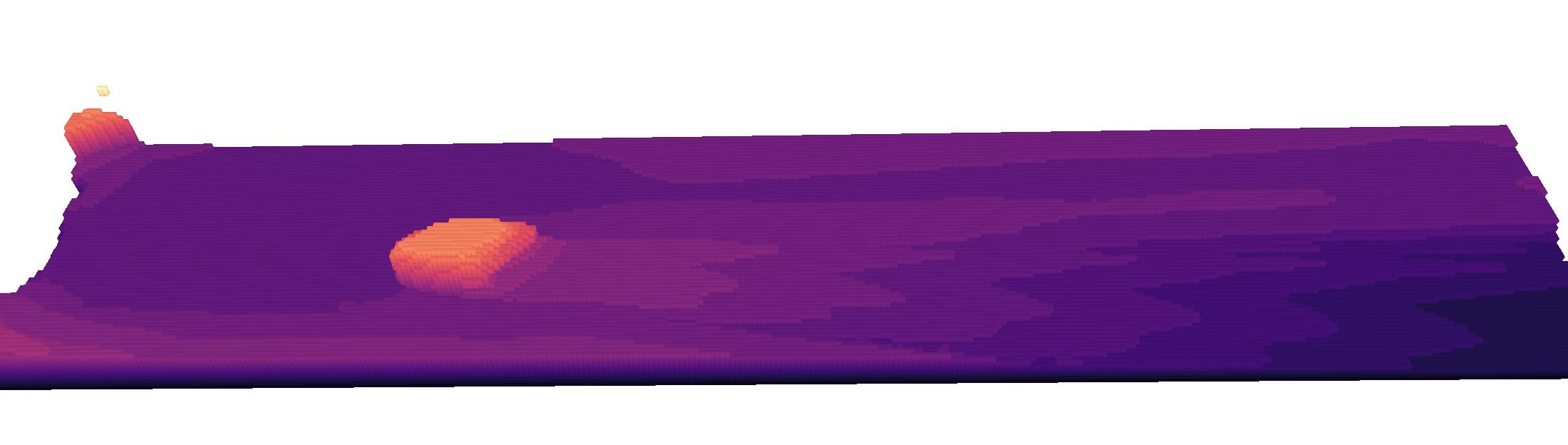
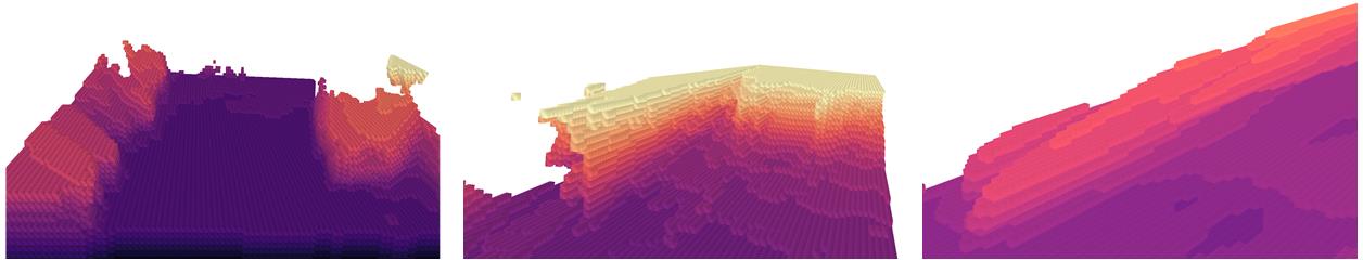
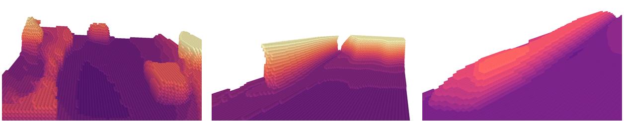
We compare our method with recent single-view scene reconstruction methods using self-supervision [17, 59, 51]. Specifically, we train Monodepth2 [17] on our benchmark as the base depth estimation method. Since the depth network cannot infer occluded geometry, we use a handcraft criterion to set areas behind the depth surface as empty space (Monodepth2 + ). We also compare our method with the NeRF-based methods [59, 51] following the same training protocol. As shown in the Tab. 1, compared to previous methods, our method achieves both the best overall performance (O) and the best occluded area reconstruction (IE, IE). Note that Monodepth2 (+ ) also yields a competitive performance in terms of invisible and empty space reconstruction (IE), but it relies on hand-crafted criteria that cannot learn true 3D in the scene. Qualitative comparisons are shown in Fig. 4. We show the reconstructed occupancy grids, where the camera is on the left side and points to the right along the -axis within [4, 50m] range. Our method demonstrates obvious qualitative superiority in reasoning occluded object shapes against the inherent ambiguity. Notably, it substantially reduces the trailing effects.
| Method | O | IE | IE | |
|---|---|---|---|---|
| 4-20m | Monodepth2 [17] | 0.69 | n/a | n/a |
| Monodepth2 [17] + | 0.70 | 0.53 | 0.52 | |
| PixelNeRF [59] | 0.67 | 0.53 | 0.49 | |
| BTS [51] | 0.79 | 0.69 | 0.60 | |
| Ours | 0.80 | 0.69 | 0.70 | |
| 4-50m | Monodepth2 [17] | 0.65 | n/a | n/a |
| Monodepth2 [17] + | 0.68 | 0.48 | 0.59 | |
| PixelNeRF [59] | 0.66 | 0.56 | 0.58 | |
| BTS [51] | 0.72 | 0.61 | 0.48 | |
| Ours | 0.75 | 0.64 | 0.68 | |
4.5 Object Reconstruction
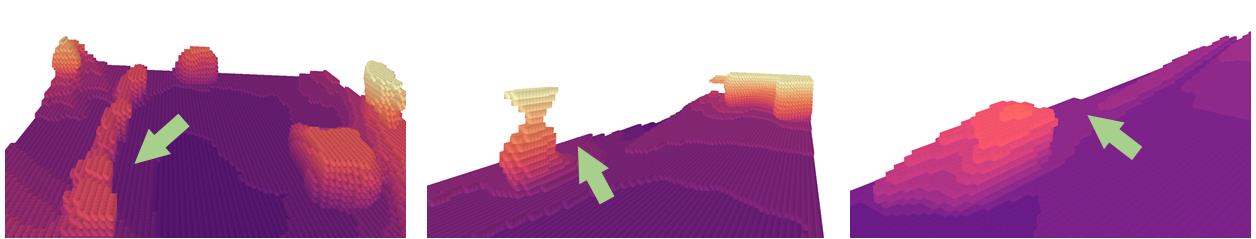
We evaluate the object reconstruction performance by computing the metrics within the annotated object areas. As shown in Tab. 2, our method achieves competitive or better results in the [4, 20m] evaluation range. Meanwhile, it achieves obvious improvements for all metrics in the [4, 50m] range, demonstrating its effectiveness in reasoning ambiguous geometries away from the camera origin. We further show reconstructions of different categories in Fig. 5. Our method generates faithful object shapes with reasonable estimates of occluded geometry for different categories including fences, trees, cars, etc., showing clear improvements over existing methods.
4.6 Ablation Studies
We evaluate the effectiveness of each contribution by separately ablating the \acvl modulation (Sec. 4.6.1) and the \acvl spatial attention (Sec. 4.6.2). We further compare with existing techniques injecting semantics from related tasks (Sec. 4.6.3). Moreover, we show our method’s improvement under a broader supervision range (Sec. 4.6.4).
4.6.1 Ablation study on VL Modulation
We evaluate the effectiveness of \acvl modulation by adding different components upon baseline method [51], which uses only appearance feature from the generic backbone [21]. In Tab. 3, we enhance the baseline by incorporating the fused \acvl image features () and injecting image/text semantics with the \acvl Modulation (VL-Mod.). We find that merely using the fused feature from the \acvl image encoder does not contribute to overall improvement. As a comparison, the proposed VL Modulation significantly improves the performances by properly interacting with image and text features.
| VL-Mod. | Scene Recon. | Object Recon. | ||||||
|---|---|---|---|---|---|---|---|---|
| O | IE | IE | O | IE | IE | |||
| ✓ | 0.84 | 0.60 | 0.53 | 0.72 | 0.61 | 0.48 | ||
| ✓ | 0.84 | 0.60 | 0.55 | 0.72 | 0.61 | 0.48 | ||
| ✓ | ✓ | 0.85 | 0.63 | 0.64 | 0.73 | 0.63 | 0.59 | |
| VL-Mod. | Attn. | VL-Attn. | Scene Recon. | Object Recon. | ||||||
| O | IE | IE | O | IE | IE | |||||
| ✓ | 0.84 | 0.60 | 0.53 | 0.72 | 0.61 | 0.48 | ||||
| ✓ | ✓ | 0.85 | 0.61 | 0.60 | 0.73 | 0.61 | 0.56 | |||
| ✓ | ✓ | 0.85 | 0.61 | 0.67 | 0.72 | 0.60 | 0.62 | |||
| ✓ | ✓ | 0.85 | 0.60 | 0.66 | 0.73 | 0.62 | 0.61 | |||
| ✓ | ✓ | ✓ | 0.86 | 0.63 | 0.75 | 0.74 | 0.62 | 0.73 | ||
| ✓ | ✓ | ✓ | 0.86 | 0.63 | 0.73 | 0.75 | 0.63 | 0.68 | ||
4.6.2 Ablation Study on Spatial Attention
In Tab. 4, we provide experimental support for the effectiveness of using spatial context, both via spatial attention and \acvl spatial attention. We first add spatial attention over image appearance features only (row: 12). Without the \acvl features, aggregating spatial context still yields notable improvement. We further show that the introduction of semantics via \acvl modulation (VL-Mod) helps independent of the spatial aggregation mechanism (row 35, row: 46), underpinning that adding VL text features outperforms using VL image features only. When combining both \acvl modulation and spatial attention mechanisms, we achieve the best performances (rows 5, 6). Additionally, we observe a small albeit notable gain when also injecting VL features into the spatial aggregation (VL-Attn), however, mainly improving details are not captured in current metrics. Please refer to the supplementary material for details.
| Semantics | Method | O | IE | IE |
|---|---|---|---|---|
| – | Baseline | 0.84 | 0.60 | 0.52 |
| Semantic Feat. | Plain Fusion | 0.84 | 0.61 | 0.51 |
| 2D Fusion - LDLS [32] | 0.84 | 0.60 | 0.55 | |
| 2D Fusion - SAFENet [8] | 0.84 | 0.60 | 0.51 | |
| VL Feat. | Fusing \acvl image feature | 0.84 | 0.60 | 0.55 |
| Ours | 0.86 | 0.63 | 0.73 |
4.6.3 Comparison with Other Semantic Guidances
As semantic cues are vital in other tasks such as depth estimation, we investigate whether the techniques used in the related literature [32, 8] are useful for single-view scene reconstruction. We use the pre-trained DPT [43] semantic network to provide pre-trained semantic features, and incorporate different feature fusion techniques [32, 8] to our density prediction pipeline. As shown in Tab. 6, we find that conducting 2D feature fusion does not lead to notable improvements over the baseline, which is consistent even with incorporating \acvl image feature fusion. However, by appropriately interacting with image and text features with 3D context awareness, our method outperforms related techniques by a notable margin.
| Supervision | Method | Scene Recon. | Object Recon. | ||||
|---|---|---|---|---|---|---|---|
| O | IE | IE | O | IE | IE | ||
| 1 in the future | BTS [51] | 0.84 | 0.61 | 0.53 | 0.72 | 0.61 | 0.48 |
| Ours | 0.86 | 0.63 | 0.73 | 0.75 | 0.64 | 0.68 | |
| 1-4 in the future | BTS [51] | 0.86 | 0.68 | 0.72 | 0.74 | 0.64 | 0.75 |
| Ours | 0.87 | 0.69 | 0.77 | 0.78 | 0.68 | 0.75 | |
4.6.4 Improvement with Broader Supervision Range
As single-view reconstruction is supervised by multiple posed images, the performance can be improved by expanding the supervisory range during training. To this end, we investigate if our method can achieve consistent improvement using a broader supervisory range. In standard supervision, we use fisheye views at the next time step (1 in the future). In the broader supervisory range, we randomly incorporate fisheye views within the next [1-4] timestep, yielding diverse supervisory ranges with a maximum coverage of 40m. We compare with BTS [51] in Tab. 6. Our method with the standard supervisory range produces comparable results to [51] with a broader supervision range. Enhanced by a broader range of supervision, our method achieves further improvement over [51].
4.7 Zero-shot Generalization on DDAD
We evaluate the zero-shot generalization of KITTI-360 trained models on the DDAD dataset. We report the meters range scene reconstruction scores in Tab. 7. Our method outperforms previous work, showing the effectiveness of the \acvl guidance for zero-shot generalization.
5 Conclusion
In this paper, we proposed \ackyn, a new method for single-view reconstruction that estimates the density of a 3D point by reasoning about its neighboring semantic and spatial context. To this end, we incorporate a \acvl modulation module to enrich 3D point representations with fine-grained semantic information. We further propose a \acvl spatial attention mechanism that makes the per-point density predictions aware of the 3D semantic context. Our approach overcomes the limitations of prior art [51], which treated the density prediction of each point independently from neighboring points and lacked explicit semantic modeling. Extensive experiments demonstrate that endowing \ackyn with semantic and contextual knowledge improves both scene and object-level reconstruction. Moreover, we find that \ackyn better generalizes out-of-domain, thanks to the proposed modulation of point representations with strong vision-language features. The incorporation of \acvl features not only enhances the performance of \ackyn, but also holds the potential to pave the way towards more general and open-vocabulary 3D scene reconstruction and segmentation techniques.
References
- Bhat et al. [2021] Shariq Farooq Bhat, Ibraheem Alhashim, and Peter Wonka. Adabins: Depth estimation using adaptive bins. In Proceedings of the IEEE/CVF Conference on Computer Vision and Pattern Recognition, pages 4009–4018, 2021.
- Bhat et al. [2022] Shariq Farooq Bhat, Ibraheem Alhashim, and Peter Wonka. Localbins: Improving depth estimation by learning local distributions. In European Conference on Computer Vision, pages 480–496. Springer, 2022.
- Bhat et al. [2023] Shariq Farooq Bhat, Reiner Birkl, Diana Wofk, Peter Wonka, and Matthias Müller. Zoedepth: Zero-shot transfer by combining relative and metric depth. arXiv preprint arXiv:2302.12288, 2023.
- Cao and de Charette [2022] Anh-Quan Cao and Raoul de Charette. Monoscene: Monocular 3d semantic scene completion. In Proceedings of the IEEE/CVF Conference on Computer Vision and Pattern Recognition, pages 3991–4001, 2022.
- Casser et al. [2019] Vincent Casser, Soeren Pirk, Reza Mahjourian, and Anelia Angelova. Depth prediction without the sensors: Leveraging structure for unsupervised learning from monocular videos. In Proceedings of the AAAI Conference on Artificial Intelligence, pages 8001–8008, 2019.
- Cheng et al. [2024a] Junda Cheng, Gangwei Xu, Peng Guo, and Xin Yang. Coatrsnet: Fully exploiting convolution and attention for stereo matching by region separation. International Journal of Computer Vision, 132(1):56–73, 2024a.
- Cheng et al. [2024b] JunDa Cheng, Wei Yin, Kaixuan Wang, Xiaozhi Chen, Shijie Wang, and Xin Yang. Adaptive fusion of single-view and multi-view depth for autonomous driving. arXiv preprint arXiv:2403.07535, 2024b.
- Choi et al. [2020] Jaehoon Choi, Dongki Jung, Donghwan Lee, and Changick Kim. Safenet: Self-supervised monocular depth estimation with semantic-aware feature extraction. arXiv preprint arXiv:2010.02893, 2020.
- Cordts et al. [2016] Marius Cordts, Mohamed Omran, Sebastian Ramos, Timo Rehfeld, Markus Enzweiler, Rodrigo Benenson, Uwe Franke, Stefan Roth, and Bernt Schiele. The cityscapes dataset for semantic urban scene understanding. In Proceedings of the IEEE conference on computer vision and pattern recognition, pages 3213–3223, 2016.
- Deng et al. [2009] Jia Deng, Wei Dong, Richard Socher, Li-Jia Li, Kai Li, and Li Fei-Fei. Imagenet: A large-scale hierarchical image database. In 2009 IEEE conference on computer vision and pattern recognition, pages 248–255. Ieee, 2009.
- Eigen et al. [2014] David Eigen, Christian Puhrsch, and Rob Fergus. Depth map prediction from a single image using a multi-scale deep network. In Advances in neural information processing systems, pages 2366–2374, 2014.
- Facil et al. [2019] Jose M Facil, Benjamin Ummenhofer, Huizhong Zhou, Luis Montesano, Thomas Brox, and Javier Civera. Cam-convs: Camera-aware multi-scale convolutions for single-view depth. In Proceedings of the IEEE/CVF Conference on Computer Vision and Pattern Recognition, pages 11826–11835, 2019.
- Feng et al. [2022] Ziyue Feng, Liang Yang, Longlong Jing, Haiyan Wang, YingLi Tian, and Bing Li. Disentangling object motion and occlusion for unsupervised multi-frame monocular depth. arXiv preprint arXiv:2203.15174, 2022.
- Fu et al. [2018] Huan Fu, Mingming Gong, Chaohui Wang, Kayhan Batmanghelich, and Dacheng Tao. Deep ordinal regression network for monocular depth estimation. In Proceedings of the IEEE Conference on Computer Vision and Pattern Recognition, pages 2002–2011, 2018.
- Fu et al. [2022] Xiao Fu, Shangzhan Zhang, Tianrun Chen, Yichong Lu, Lanyun Zhu, Xiaowei Zhou, Andreas Geiger, and Yiyi Liao. Panoptic nerf: 3d-to-2d label transfer for panoptic urban scene segmentation. In 2022 International Conference on 3D Vision (3DV), pages 1–11. IEEE, 2022.
- Geiger et al. [2012] Andreas Geiger, Philip Lenz, and Raquel Urtasun. Are we ready for autonomous driving? the kitti vision benchmark suite. In 2012 IEEE Conference on Computer Vision and Pattern Recognition, pages 3354–3361. IEEE, 2012.
- Godard et al. [2019] Clément Godard, Oisin Mac Aodha, Michael Firman, and Gabriel J Brostow. Digging into self-supervised monocular depth estimation. In Proceedings of the IEEE International Conference on Computer Vision, pages 3828–3838, 2019.
- Guizilini et al. [2020a] Vitor Guizilini, Rares Ambrus, Sudeep Pillai, Allan Raventos, and Adrien Gaidon. 3d packing for self-supervised monocular depth estimation. In Proceedings of the IEEE/CVF Conference on Computer Vision and Pattern Recognition, pages 2485–2494, 2020a.
- Guizilini et al. [2020b] Vitor Guizilini, Rui Hou, Jie Li, Rares Ambrus, and Adrien Gaidon. Semantically-guided representation learning for self-supervised monocular depth. In International Conference on Learning Representations, 2020b.
- Guizilini et al. [2023] Vitor Guizilini, Igor Vasiljevic, Dian Chen, Rareș Ambruș, and Adrien Gaidon. Towards zero-shot scale-aware monocular depth estimation. In Proceedings of the IEEE/CVF International Conference on Computer Vision, pages 9233–9243, 2023.
- He et al. [2016] Kaiming He, Xiangyu Zhang, Shaoqing Ren, and Jian Sun. Deep residual learning for image recognition. In Proceedings of the IEEE conference on computer vision and pattern recognition, pages 770–778, 2016.
- Jung et al. [2021] Hyunyoung Jung, Eunhyeok Park, and Sungjoo Yoo. Fine-grained semantics-aware representation enhancement for self-supervised monocular depth estimation. In Proceedings of the IEEE/CVF International Conference on Computer Vision, pages 12642–12652, 2021.
- Katharopoulos et al. [2020] Angelos Katharopoulos, Apoorv Vyas, Nikolaos Pappas, and François Fleuret. Transformers are rnns: Fast autoregressive transformers with linear attention. In International conference on machine learning, pages 5156–5165. PMLR, 2020.
- Kerr et al. [2023] Justin Kerr, Chung Min Kim, Ken Goldberg, Angjoo Kanazawa, and Matthew Tancik. Lerf: Language embedded radiance fields. In Proceedings of the IEEE/CVF International Conference on Computer Vision, pages 19729–19739, 2023.
- Kingma and Ba [2014] Diederik P Kingma and Jimmy Ba. Adam: A method for stochastic optimization. arXiv preprint arXiv:1412.6980, 2014.
- Kundu et al. [2022] Abhijit Kundu, Kyle Genova, Xiaoqi Yin, Alireza Fathi, Caroline Pantofaru, Leonidas J Guibas, Andrea Tagliasacchi, Frank Dellaert, and Thomas Funkhouser. Panoptic neural fields: A semantic object-aware neural scene representation. In Proceedings of the IEEE/CVF Conference on Computer Vision and Pattern Recognition, pages 12871–12881, 2022.
- Lee et al. [2022] Minhyeok Lee, Sangwon Hwang, Chaewon Park, and Sangyoun Lee. Edgeconv with attention module for monocular depth estimation. In Proceedings of the IEEE/CVF Winter Conference on Applications of Computer Vision, pages 2858–2867, 2022.
- Lee et al. [2021] Seokju Lee, Sunghoon Im, Stephen Lin, and In So Kweon. Learning monocular depth in dynamic scenes via instance-aware projection consistency. arXiv preprint arXiv:2102.02629, 2021.
- Li et al. [2022] Boyi Li, Kilian Q Weinberger, Serge Belongie, Vladlen Koltun, and Rene Ranftl. Language-driven semantic segmentation. In International Conference on Learning Representations, 2022.
- Li et al. [2020] Rui Li, Xiantuo He, Yu Zhu, Xianjun Li, Jinqiu Sun, and Yanning Zhang. Enhancing self-supervised monocular depth estimation via incorporating robust constraints. In Proceedings of the 28th ACM International Conference on Multimedia, pages 3108–3117, 2020.
- Li et al. [2023a] Rui Li, Dong Gong, Wei Yin, Hao Chen, Yu Zhu, Kaixuan Wang, Xiaozhi Chen, Jinqiu Sun, and Yanning Zhang. Learning to fuse monocular and multi-view cues for multi-frame depth estimation in dynamic scenes. In Proceedings of the IEEE/CVF Conference on Computer Vision and Pattern Recognition, pages 21539–21548, 2023a.
- Li et al. [2023b] Rui Li, Danna Xue, Shaolin Su, Xiantuo He, Qing Mao, Yu Zhu, Jinqiu Sun, and Yanning Zhang. Learning depth via leveraging semantics: Self-supervised monocular depth estimation with both implicit and explicit semantic guidance. Pattern Recognition, page 109297, 2023b.
- Liang et al. [2023] Jingyun Liang, Yuchen Fan, Kai Zhang, Radu Timofte, Luc Van Gool, and Rakesh Ranjan. Movideo: Motion-aware video generation with diffusion models. arXiv preprint arXiv:2311.11325, 2023.
- Liao et al. [2022] Yiyi Liao, Jun Xie, and Andreas Geiger. Kitti-360: A novel dataset and benchmarks for urban scene understanding in 2d and 3d. IEEE Transactions on Pattern Analysis and Machine Intelligence, 45(3):3292–3310, 2022.
- Liu et al. [2023a] Ce Liu, Suryansh Kumar, Shuhang Gu, Radu Timofte, and Luc Van Gool. Single image depth prediction made better: A multivariate gaussian take. In Proceedings of the IEEE/CVF Conference on Computer Vision and Pattern Recognition, pages 17346–17356, 2023a.
- Liu et al. [2023b] Ce Liu, Suryansh Kumar, Shuhang Gu, Radu Timofte, and Luc Van Gool. Va-depthnet: A variational approach to single image depth prediction. arXiv preprint arXiv:2302.06556, 2023b.
- Lyu et al. [2020] Xiaoyang Lyu, Liang Liu, Mengmeng Wang, Xin Kong, Lina Liu, Yong Liu, Xinxin Chen, and Yi Yuan. Hr-depth: High resolution self-supervised monocular depth estimation. arXiv preprint arXiv:2012.07356, 2020.
- Miao et al. [2023] Ruihang Miao, Weizhou Liu, Mingrui Chen, Zheng Gong, Weixin Xu, Chen Hu, and Shuchang Zhou. Occdepth: A depth-aware method for 3d semantic scene completion. arXiv preprint arXiv:2302.13540, 2023.
- Mildenhall et al. [2020] Ben Mildenhall, Pratul P. Srinivasan, Matthew Tancik, Jonathan T. Barron, Ravi Ramamoorthi, and Ren Ng. Nerf: Representing scenes as neural radiance fields for view synthesis. In ECCV, 2020.
- Paszke et al. [2017] Adam Paszke, Sam Gross, Soumith Chintala, Gregory Chanan, Edward Yang, Zachary DeVito, Zeming Lin, Alban Desmaison, Luca Antiga, and Adam Lerer. Automatic differentiation in pytorch. 2017.
- Peng et al. [2023] Songyou Peng, Kyle Genova, Chiyu Jiang, Andrea Tagliasacchi, Marc Pollefeys, Thomas Funkhouser, et al. Openscene: 3d scene understanding with open vocabularies. In Proceedings of the IEEE/CVF Conference on Computer Vision and Pattern Recognition, pages 815–824, 2023.
- Ranftl et al. [2020] René Ranftl, Katrin Lasinger, David Hafner, Konrad Schindler, and Vladlen Koltun. Towards robust monocular depth estimation: Mixing datasets for zero-shot cross-dataset transfer. IEEE transactions on pattern analysis and machine intelligence, 44(3):1623–1637, 2020.
- Ranftl et al. [2021] René Ranftl, Alexey Bochkovskiy, and Vladlen Koltun. Vision transformers for dense prediction. In Proceedings of the IEEE/CVF international conference on computer vision, pages 12179–12188, 2021.
- Schmied et al. [2023] Aron Schmied, Tobias Fischer, Martin Danelljan, Marc Pollefeys, and Fisher Yu. R3d3: Dense 3d reconstruction of dynamic scenes from multiple cameras. In Proceedings of the IEEE/CVF International Conference on Computer Vision, pages 3216–3226, 2023.
- Shen et al. [2021] Zhuoran Shen, Mingyuan Zhang, Haiyu Zhao, Shuai Yi, and Hongsheng Li. Efficient attention: Attention with linear complexities. In Proceedings of the IEEE/CVF winter conference on applications of computer vision, pages 3531–3539, 2021.
- Spencer et al. [2023] Jaime Spencer, Chris Russell, Simon Hadfield, and Richard Bowden. Kick back & relax: Learning to reconstruct the world by watching slowtv. In Proceedings of the IEEE/CVF International Conference on Computer Vision, pages 15768–15779, 2023.
- Sun et al. [2023] Libo Sun, Jia-Wang Bian, Huangying Zhan, Wei Yin, Ian Reid, and Chunhua Shen. Sc-depthv3: Robust self-supervised monocular depth estimation for dynamic scenes. IEEE Transactions on Pattern Analysis and Machine Intelligence, 2023.
- Teed and Deng [2018] Zachary Teed and Jia Deng. Deepv2d: Video to depth with differentiable structure from motion. arXiv preprint arXiv:1812.04605, 2018.
- Wang et al. [2021a] Peng Wang, Lingjie Liu, Yuan Liu, Christian Theobalt, Taku Komura, and Wenping Wang. Neus: Learning neural implicit surfaces by volume rendering for multi-view reconstruction. arXiv preprint arXiv:2106.10689, 2021a.
- Wang et al. [2021b] Qianqian Wang, Zhicheng Wang, Kyle Genova, Pratul P Srinivasan, Howard Zhou, Jonathan T Barron, Ricardo Martin-Brualla, Noah Snavely, and Thomas Funkhouser. Ibrnet: Learning multi-view image-based rendering. In Proceedings of the IEEE/CVF Conference on Computer Vision and Pattern Recognition, pages 4690–4699, 2021b.
- Wimbauer et al. [2023] Felix Wimbauer, Nan Yang, Christian Rupprecht, and Daniel Cremers. Behind the scenes: Density fields for single view reconstruction. In Proceedings of the IEEE/CVF Conference on Computer Vision and Pattern Recognition, pages 9076–9086, 2023.
- Xian et al. [2020] Ke Xian, Jianming Zhang, Oliver Wang, Long Mai, Zhe Lin, and Zhiguo Cao. Structure-guided ranking loss for single image depth prediction. In Proceedings of the IEEE/CVF Conference on Computer Vision and Pattern Recognition, pages 611–620, 2020.
- Xu et al. [2022] Gangwei Xu, Junda Cheng, Peng Guo, and Xin Yang. Attention concatenation volume for accurate and efficient stereo matching. In Proceedings of the IEEE/CVF conference on computer vision and pattern recognition, pages 12981–12990, 2022.
- Yariv et al. [2021] Lior Yariv, Jiatao Gu, Yoni Kasten, and Yaron Lipman. Volume rendering of neural implicit surfaces. Advances in Neural Information Processing Systems, 34:4805–4815, 2021.
- Yin et al. [2019] Wei Yin, Yifan Liu, Chunhua Shen, and Youliang Yan. Enforcing geometric constraints of virtual normal for depth prediction. In Proceedings of the IEEE/CVF International Conference on Computer Vision, pages 5684–5693, 2019.
- Yin et al. [2021] Wei Yin, Jianming Zhang, Oliver Wang, Simon Niklaus, Long Mai, Simon Chen, and Chunhua Shen. Learning to recover 3d scene shape from a single image. In Proceedings of the IEEE/CVF Conference on Computer Vision and Pattern Recognition, pages 204–213, 2021.
- Yin et al. [2022] Wei Yin, Jianming Zhang, Oliver Wang, Simon Niklaus, Simon Chen, Yifan Liu, and Chunhua Shen. Towards accurate reconstruction of 3d scene shape from a single monocular image. IEEE Transactions on Pattern Analysis and Machine Intelligence, 2022.
- Yin et al. [2023] Wei Yin, Chi Zhang, Hao Chen, Zhipeng Cai, Gang Yu, Kaixuan Wang, Xiaozhi Chen, and Chunhua Shen. Metric3d: Towards zero-shot metric 3d prediction from a single image. In Proceedings of the IEEE/CVF International Conference on Computer Vision, pages 9043–9053, 2023.
- Yu et al. [2021] Alex Yu, Vickie Ye, Matthew Tancik, and Angjoo Kanazawa. pixelnerf: Neural radiance fields from one or few images. In Proceedings of the IEEE/CVF Conference on Computer Vision and Pattern Recognition, pages 4578–4587, 2021.
- Yu et al. [2022] Zehao Yu, Songyou Peng, Michael Niemeyer, Torsten Sattler, and Andreas Geiger. Monosdf: Exploring monocular geometric cues for neural implicit surface reconstruction. Advances in neural information processing systems, 35:25018–25032, 2022.
- Yuan et al. [2022] Weihao Yuan, Xiaodong Gu, Zuozhuo Dai, Siyu Zhu, and Ping Tan. New crfs: Neural window fully-connected crfs for monocular depth estimation. arXiv preprint arXiv:2203.01502, 2022.
- Zhao et al. [2022] Chaoqiang Zhao, Youmin Zhang, Matteo Poggi, Fabio Tosi, Xianda Guo, Zheng Zhu, Guan Huang, Yang Tang, and Stefano Mattoccia. Monovit: Self-supervised monocular depth estimation with a vision transformer. In 2022 International Conference on 3D Vision (3DV), pages 668–678. IEEE, 2022.
- Zhi et al. [2021] Shuaifeng Zhi, Tristan Laidlow, Stefan Leutenegger, and Andrew J Davison. In-place scene labelling and understanding with implicit scene representation. In Proceedings of the IEEE/CVF International Conference on Computer Vision, pages 15838–15847, 2021.
- Zhou et al. [2021] Hang Zhou, David Greenwood, and Sarah Taylor. Self-supervised monocular depth estimation with internal feature fusion. arXiv preprint arXiv:2110.09482, 2021.