Magnetic fields from small-scale primordial perturbations
Abstract
Weak magnetic fields must have existed in the early Universe, as they were sourced by the cross product of electron density and temperature gradients through the Biermann-battery mechanism. In this paper we calculate the magnetic fields generated at cosmic dawn by a variety of small-scale primordial perturbations, carefully computing the evolution of electron density and temperature fluctuations, and consistently accounting for relative velocities between baryons and dark matter. We first compute the magnetic field resulting from standard, nearly scale-invariant primordial adiabatic perturbations, making significant improvements to previous calculations. This “standard” primordial field has a root mean square (rms) of a few times nG at , with fluctuations on kpc comoving scales, and could serve as the seed of present-day magnetic fields observed in galaxies and galaxy clusters. In addition, we consider early-Universe magnetic fields as a possible probe of non-standard initial conditions of the Universe on small scales Mpc-1. To this end, we compute the maximally-allowed magnetic fields within current upper limits on small-scale adiabatic and isocurvature perturbations. Enhanced small-scale adiabatic fluctuations below current Cosmic Microwave Background spectral-distortion constraints could produce magnetic fields as large as nG at . Uncorrelated small-scale isocurvature perturbations within current Big-Bang Nucleosynthesis bounds could potentially enhance the rms magnetic field to nG at , depending on the specific isocurvature mode considered. While these very weak fields remain well below current observational capabilities, our work points out that magnetic fields could potentially provide an interesting window into the poorly constrained small-scale initial conditions of the Universe.
I Introduction
While magnetic fields are ubiquitous in the Universe Vallée (2004); Neronov and Vovk (2010); Beck (2012); Durrer and Neronov (2013), their origin remains unknown. A possible explanation could be the dynamo amplification of “primordial” magnetic fields, generated in the early Universe prior to non-linear structure formation Durrer and Neronov (2013). Indeed, even seed magnetic fields as weak as nG at the time of galaxy formation could be sufficient to source the magnetic fields observed today in galaxies and galaxy clusters Davis et al. (1999).
In 1950, Biermann showed that magnetic fields can be generated starting from vanishing initial conditions in an ionized plasma if the electron density and temperature gradients are misaligned Biermann (1950), a process now known as the Biermann-battery mechanism. About a decade ago, Naoz and Narayan Naoz and Narayan (NN13) (hereafter NN13), considered this mechanism within a cosmological context for the first time. They computed the magnetic field sourced by linear fluctuations originating from adiabatic initial conditions, assuming the latter have a nearly scale-invariant power spectrum with amplitude and slope consistent with large-scale Cosmic Microwave Background (CMB) anisotropy data. They found that these “standard” adiabatic initial conditions could lead to a magnetic field with root-mean-square (rms) nG at redshift , fluctuating on comoving scales of order kpc. NN13 accounted approximately for the effect of supersonic relative motions between baryons and cold dark matter (CDM) Tseliakhovich and Hirata (2010), which they showed to significantly affect the resulting magnetic field power spectrum.
A byproduct of NN13’s work is the understanding that the cosmological Biermann-battery mechanism is most efficient on 1–10 kpc comoving scales. This implies that the resulting magnetic field could, in principle, offer a window into initial conditions on these scales, much smaller and much more poorly constrained than the Mpc scales directly probed by CMB-anisotropy and large-scale structure data. Not only could kpc-scale initial conditions have a significantly larger amplitude than their Mpc–Gpc scale counterparts, they may also depart significantly from adiabaticity, since isocurvature (i.e. non-adiabatic) initial conditions are especially weakly constrained on such scales. The purpose of the present paper is to compute the magnetic field generated by non-standard initial conditions through the Biermann-battery mechanism, in the hopes that this observable may eventually serve as a probe of the small-scale primordial Universe.
A related endeavor was recently undertaken by Flitter et al. Flitter et al. (2023) (hereafter F+23), whose work inspired ours. Specifically, F+23 computed the magnetic field sourced by small-scale compensated isocurvature perturbations (CIPs), in which initial baryon and CDM perturbations compensate each other to produce an exactly vanishing total matter fluctuation. In this work, we significantly expand on F+23’s calculation in multiple aspects. First and foremost, we consider a variety of isocurvature initial conditions in addition to CIPs, as well as amplified small-scale adiabatic initial conditions. Second, we numerically evolve linear electron density and temperature fluctuations, rather than using simple analytic approximations which can be inaccurate by up to one order of magnitude. Last but not least, we incorporate exactly the effect of large-scale relative motions between baryons and CDM, which significantly affect the growth of small-scale perturbations, be they originated from adiabatic or isocurvature initial conditions. Along the way, we also make some significant improvements to NN13’s original work. We update their prediction for the magnetic field sourced by standard adiabatic initial conditions, which we find can reach root-mean-square (rms) of nG at , peaking at , assuming small-scale initial conditions consistent with the Planck 2018 best-fit cosmology Aghanim et al. (2020).
Our main result is to predict the magnetic field produced by non-standard small-scale perturbations, and can be summarized as follows. We find that enhanced small-scale adiabatic initial conditions can lead to magnetic fields as large as nG without violating CMB spectral-distortion constraints Chluba and Grin (2013). We also show that, within current constraints, small-scale isocurvature perturbations may source magnetic fields reaching nG at , depending on the specific type of isocurvature mode. We note that our more accurate treatment leads to a prediction for the magnetic field sourced by CIPs up to one order of magnitude larger than that of F+23. Although to our knowledge no observational method currently exists to probe such weak small-scale magnetic fields at cosmic dawn (but see Ref. Venumadhav et al. (2017); Gluscevic et al. (2017) for a probe of large-scale magnetic fields of comparable magnitude), these field amplitudes are in principle large enough to seed magnetic fields observed in today’s galaxies and galaxy clusters, and can be significantly larger than the expectation from standard adiabatic initial conditions.
The rest of this paper is organized as follows. In Sec. II, we describe how we calculate perturbations in electron density and baryonic gas temperature, which are the principal ingredients of the Biermann-battery mechanism, including the effect of relative velocity between CDM and baryons. In Sec. III we derive the power spectrum of the magnetic field sourced by general electron and temperature fluctuations through the Biermann-battery mechanism, and present our results with standard primordial adiabatic perturbations. In Sec. IV we consider non-standard adiabatic and isocurvature initial conditions saturating current constraints, and compute the resulting magnetic field power spectrum. We conclude in Sec. V. We give a pedagogical derivation of the Biermann-battery mechanism in a cosmological context in Appendix A, provide details of our numerical implementation in Appendix B, and give a detailed comparison of our work with that of F+23 in Appendix C.
II Evolution of Perturbations
II.1 Implementation
In this section we describe how we compute the linear evolution of perturbations in CDM, baryons, free electron fraction , and gas temperature , the latter two being relevant to the computation of magnetic fields. We separate perturbations into “large scales” and “small scales”, depending on whether their comoving wavenumber is less or greater than 1 Mpc-1, respectively.
On large scales, perturbations are insensitive to relative velocities between baryons and CDM (their effect is only relevant at Mpc-1 Tseliakhovich and Hirata (2010)). Moreover, baryon pressure is negligible, and as a consequence free-electron and gas temperature fluctuations do not affect the evolution of large-scale perturbations at linear level (even though the converse is true). We may therefore obtain the evolution of baryon density and velocity perturbations from the Boltzmann code class Blas et al. (2011), and compute the linear response of the free-electron fraction and gas temperature to these perturbations using the modified recombination code hyrec-2 Ali-Haimoud and Hirata (2010, 2011); Lee and Ali-Haïmoud (2020), with the method described in Ref. Lee and Ali-Haïmoud (2021). This allows us to extract the relative perturbations and as a function of time (or redshift) and wavenumber, for any given initial conditions.
The same is approximately true for the evolution of small-scale perturbations prior to kinematic decoupling of baryons from photons, at , since at that epoch the dynamics of baryons is dominated by their coupling to photons. Therefore, we also use class combined with the modified hyrec-2 linear-response solution for for small-scale perturbations111While perturbed recombination calculations Naoz and Barkana (2005); Lewis (2007); Senatore et al. (2009) are available in class, in its default setting the code works only for relatively large-scale modes. Moreover, the perturbed recombination equation implemented in class are only valid in the limit when photoionizations are negligible, and after transitions from the excited to the ground state are no longer bottlenecked, i.e. for . Except for our neglect of photon perturbations in the gas temperature evolution, our implementation with the modified hyrec-2 is therefore more accurate. until . After photon-baryon kinematic decoupling, baryon pressure becomes relevant, and as consequence the evolution of baryon fluid variables becomes coupled to gas temperature fluctuations, which are themselves coupled to free-electron fraction fluctuations. Moreover, relative velocities between baryons and CDM affect the growth of small-scale perturbations, as they advect baryon and CDM perturbations relative to one another Tseliakhovich and Hirata (2010). Since the effect of baryon-CDM relative velocities is non-linear and not included into class, we implement our own differential equation solver, initialized with our class + modified hyrec-2 solution at . We follow the treatment of Refs. Tseliakhovich and Hirata (2010); Ali-Haïmoud et al. (2014). Given that scales Mpc-1 are well within the horizon scale at , we may solve the fluid equations in the subhorizon limit. We may also neglect photon perturbations, due to their rapid free-streaming. Moreover, given that relative velocities fluctuate on scales Mpc-1, and only affect perturbations on scales Mpc-1, we may use moving-background perturbation theory Tseliakhovich and Hirata (2010), by solving for the evolution of small-scale perturbations on a local patch of uniform relative velocity , in the baryon’s rest-frame. Explicitly, we solve the following system of coupled differential equations for the baryon and CDM density perturbations () and velocity divergences with respect to proper space (, as well gas temperature and ionization fraction perturbations , where overdots denote derivatives with respect to coordinate time:
| (1) | |||||
In these equations, all quantities except for the perturbation variables are by default background (i.e. homogeneous) quantities, is the Hubble rate, and are the contributions of baryons and CDM to the total critical energy density. We calculate the background gas temperature and free electron fraction using the recombination code hyrec-2 Ali-Haimoud and Hirata (2010, 2011); Lee and Ali-Haïmoud (2020) implemented in class Blas et al. (2011). The last term in the baryon momentum equation, proportional to the background electron density and the Thomson scattering cross section , accounts for residual photon drag after , and is required to obtain accurate results, especially for non-adiabatic initial conditions. The baryon’s isothermal sound speed squared is given by , where is the mean molecular weight which depends on the background free-electron fraction and the constant ratio of helium to hydrogen by number . Note that we do not include fluctuations of the molecular weight since and free-electron fraction fluctuations remain very small at the redshifts of interest Ali-Haïmoud et al. (2014). The evolution of gas temperature perturbations is governed by the Compton heating rate
| (2) |
and the evolution of ionization perturbations depends on the effective case-B recombination coefficient Ali-Haimoud and Hirata (2010), as well as on the corresponding effective photoionization rate through Peebles’ -factor Peebles (1968)
| (3) |
where is the two-photon decay rate, and is the Lyman- net decay rate defined as
| (4) |
where is the number density of hydrogen.
Note that the equation for ionization fraction perturbations is only valid for scales larger than the typical distance travelled by Lyman- photons between emission and absorption events, i.e. for scales Mpc-1 Venumadhav and Hirata (2015). We will extrapolate our results to scales Mpc-1, but the reader should keep in mind that they can only be fully trusted for Mpc-1.
II.2 Initial conditions and results
We consider five types of primordial perturbations (defined at , prior to horizon entry): adiabatic (AD), baryon isocurvature (BI), CDM isocurvature (CI), joint baryon and CDM isocurvature (BCI), and compensated isocurvature perturbations (CIPs). For BCI, baryons and CDM perturbations are initially equal, while for CIPs, initially, such that baryons and CDM produce no net gravitational potential. Let us note that, in principle, all primordial perturbations may contribute to large-scale relative velocities. However, we checked that the dominant contribution is always coming from adiabatic perturbations under current constraints on the amplitude of large-scale primordial perturbations. Hence, regardless of the type of small-scale initial conditions considered when solving Eqs. (1), the relative velocity of CDM and baryon is always assumed to be determined by that of adiabatic perturbations.
Each type of initial condition is characterized by a single scalar variable , which is the primordial curvature perturbation for adiabatic initial conditions, the initial baryon density for BI, BCI and CIP, and the initial CDM density for CI. The output of our code are the transfer functions of each variable , for each type of initial conditions, defined through
| (5) |
where (which we will simply denote by in what follows) is the local baryon-CDM relative velocity at , which affects perturbations of wave-vector only through its projection along . As a cross check of our code, we have explicitly computed the matter power spectrum for adiabatic initial conditions, averaged it over the Gaussian distribution of relative velocities, and confirmed it agrees with the results of Ref. Tseliakhovich and Hirata (2010).
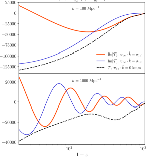
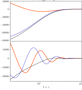
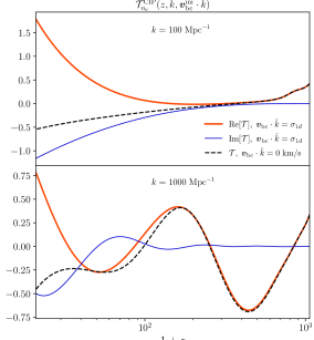
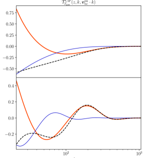
In the context of magnetic fields, we are especially interested in the transfer functions of the gas temperature perturbation and of the free-electron density perturbation , since these are the relevant fields for the Biermann-battery mechanism. We show some of these transfer functions in Fig. 1 for AD and CIP modes.
III Magnetic field from the Biermann-battery mechanism
III.1 General expressions
The Biermann-battery mechanism sources a magnetic field at a rate proportional to the cross product of the free-electron density and temperature gradients. In the expanding Universe, this rate is Naoz and Narayan (NN13); Papanikolaou and Gourgouliatos (2023); Flitter et al. (2023)
| (6) |
where is the electron charge (see Appendix A for a pedagogical derivation). We may easily integrate this equation, and write its explicit solution in Fourier space, for a given initial value of the local relative velocity :
| (7) |
Recalling the definition of the transfer functions in Eq. (5), and accounting for a possible superposition of multiple types of initial conditions, we get
| (8) |
where AD, BI, CI, BCI, CIP, and we have defined
| (9) |
We see that, for a given realization of the initial conditions, depends on the full vector , in contrast with the linear fields , which only depend on .
We now compute the small-scale power spectrum of the magnetic field, for a given local value . It is defined as
| (10) |
under the assumption of Gaussian initial conditions, uncorrelated between different types:
| (11) |
Note that our calculation could easily be generalized to correlated initial conditions. Using the properties of Gaussian random fields, we arrive at
| (12) |
where we have defined
| (13) |
The local small-scale power spectrum defined in Eq. (12) is not statistically isotropic, as it depends on the direction through . Note that, unlike the matter power spectrum, which depends on relative velocity only through its projection along Tseliakhovich and Hirata (2010), the local small-scale power spectrum of the magnetic field depends on the relative magnitude and on its angle with separately, i.e. .
A more physically meaningful quantity is the direction-averaged power spectrum, which by slight abuse of notation we denote , defined as
| (14) | |||||
The isotropic magnetic field power spectrum only depends on the magnitude of the local relative velocity. Lastly, the global magnetic field power spectrum is obtained by averaging over the Gaussian distribution of relative velocities at , with variance per axis Tseliakhovich and Hirata (2010) , explicitly,
| (15) |
From the magnetic field power spectrum, one may obtain the overall variance of the magnetic field,
| (16) |
Whenever we quote our results for , we take an upper cutoff Mpc-1 in this integral.
We see that obtaining the magnetic field power spectrum at a given redshift and wavenumber requires computing a 5-dimensional integral: three angular integrals (corresponding to the relative angles between and ), one integral over the magnitude of , and one over the distribution of . Moreover, the integrand in Eq. (12) itself depends on time (or redshift) integrals of products of transfer functions. This therefore represents a very significant computational challenge, which requires careful optimization to remain tractable. We provide the details of our numerical implementation in Appendix B.
III.2 Application to nearly scale-invariant adiabatic initial conditions
In this section, we show the power spectrum of magnetic field produced by perturbations in electron density and gas temperature seeded by “standard” primordial adiabatic perturbations, with a nearly scale-invariant primordial power spectrum
| (17) |
where the pivot scale is Mpc-1, the amplitude is , and the spectral index is , which are the Planck CMB-anisotropy best-fit values.
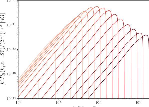
We present our result in Fig. 2, where we show the rms magnetic field per logarithmic scale, , at . We see that it peaks around comoving wavenumber , with an overall rms nG. Accounting for relative velocities does not significantly shift the peak of , but significantly enhances power on scales Mpc-1. In particular, non-vanishing relative velocities change the large-scale (small-) asymptotic scaling of from to .
These asymptotic behaviors can be understood as follows. First, let us note that the reality condition of real-space perturbations implies that for any perturbation . Therefore, .
For , all transfer functions are real, and as a consequence, , implying that, at lowest order in , for . From Eq. (12), we thus find for much smaller than the peak of the integrand (which is around the Jeans scale for adiabatic initial conditions), explaining the observed scaling . For , transfer functions acquire a non-vanishing imaginary part (see Fig. 1). This implies that . As a consequence, Eq. (12) gives for , implying , as observed in Fig. 2.

Let us recall that our results should only be trusted for Mpc-1, since for smaller scales finite photon propagation effects may significantly alter the evolution of perturbed recombination Venumadhav and Hirata (2015).
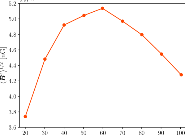
The redshift evolution of the rms magnetic field is determined by a competition between the Biermann-battery production rate and dilution by cosmological expansion. We show this evolution in Fig. 3, where we see that the rms magnetic field increases until , after which it starts decreasing. This interesting result could not easily be predicted analytically.
Our results are significantly different from those obtained in the pioneering work of NN13. Specifically, we obtain an overall magnetic field rms larger than theirs by at least one order of magnitude, and significantly different large-scale asymptotic behaviors for . We were able to identify some assumptions that may explain part of these differences. First, NN13 assume that the perturbations in free electron density are equal to the perturbations in free-electron fraction, i.e. that , instead of . However, we find that, for adiabatic perturbations, at on all scales Mpc-1. Hence, NN13’s assumption significantly underestimates the free-electron density perturbation, which may explain why they obtain a lower magnetic field amplitude than we do. Second, NN13 estimate the angle-average power spectrum by substituting222Private communication from S. Naoz. in Eq. (9), where the average is over the angle between and . This does not account for correlations between transfer functions at different wavenumbers for a given relative velocity, as is correctly accounted for when we average itself (which is quartic in transfer functions) over angles. This assumption of NN13 explains why they obtain the same large-scale asymptotic scaling for regardless of the value of : their averaging procedure spuriously eliminates the imaginary part of , which, as we show above, is responsible for the different asymptotic scaling of . Neither one of these assumptions (nor the minor differences in our evolution equations for ) explain the asymptotic behavior of found by NN13, however: their Fig. 2 shows on large scales, implying , independently of . This result is inconsistent with the fact that should scale at least quadratically in on large scales, as can be seen e.g. from Eq. (12). Our new results should thus be seen as updating and superseding those of NN13.
IV Magnetic field as a probe of small-scale initial conditions
IV.1 Setup
We now compute the magnetic field generated by the superposition of the “standard” (CMB-extrapolated) adiabatic initial conditions with power spectrum given in Eq. (17), with a non-standard power spectrum for a single type of primordial perturbation (possibly adiabatic as well) with a Dirac-delta peak at scale :
| (18) |
The resulting magnetic field power spectrum is then
| (19) | |||||
which includes the cross term, linear in ,
| (20) |
and a term quadratic in , given by
| (21) |
for , and vanishing otherwise, where is the azimuthal angle of in the spherical polar coordinate system where is the zenith, and the plane spanned by has . The term peaks near .
In what follows we apply these results to spikes in the small-scale adiabatic or isocurvature perturbations, saturating existing upper limits, to show the maximum magnetic field they might generate.
IV.2 Application to enhanced small-scale adiabatic perturbations
CMB anisotropy data only probes relatively large-scale () adiabatic modes. On smaller scales, the most stringent constraints to date can be derived from upper bounds to CMB spectra distortions. Ref. Chluba et al. (2012) provide simple analytic expressions for the chemical potential and Compton- distortion sourced by small-scale adiabatic perturbations with a Dirac-Delta spike as in Eq. (18), accurate to for Mpc-1:
| (22) | |||||
| (23) | |||||
| (24) |
COBE-FIRAS Fixsen et al. (1996) constrains and at the 95% confidence interval. This implies that, the bound on is approximately
| (25) |
This expression recovers the bounds from either or limits in the region where either one dominates.
Fig. 4 shows the velocity-averaged -field power spectrum at produced by adiabatic primordial perturbations with a Dirac-Delta spike saturating spectral distortion upper limits (in addition to the “standard” nearly scale-invariant power spectrum), for varying spike positions . We find that magnetic fields can be as large as nG, four orders of magnitude larger than that generated by standard adiabatic initial conditions, without violating CMB spectral-distortion constraints. This maximum rms is attained for Mpc-1.
IV.3 Application to small-scale isocurvature perturbations
We now compute the magnetic field power spectrum generated by various small-scale isocurvature perturbations saturating current limits. For BI, BCI and CIPs, the most stringent upper limits come from Big-Bang Nucleosynthesis (BBN) constraints, first derived in Ref. Inomata et al. (2018) and revised in Ref. Lee and Ali-Haïmoud (2021), which limit the primordial baryon variance on scales larger than the neutron diffusion scale, Mpc-1, implying
| (26) |
For pure CDM isocurvature (CI), the BBN bound does not apply. Instead, the strongest constraint is the one we obtained in Ref. Lee and Ali-Haïmoud (2021) based on the perturbation of the average recombination history, which is of order for Mpc-1, and rapidly degrades for smaller scales. Given that linear perturbation theory should not apply for such large amplitudes, the precise value of the bound is not robust. Therefore, for illustration purposes, we simply compute the magnetic field generated with .
We show in Fig. 5 the rms magnetic field generated by small-scale isocurvature perturbations saturating the limits described above, as a function of the peak scale . We find that, under current constraints, primordial isocurvature perturbations have the potential to enhance up to for BCI, nG for BI, and nG for CIP. Since CI are not well constrained on these scales, they may source a magnetic field with rms up to nG. Note that as is the dominant contribution for {BI, BCI, CI}, the rms magnetic field scales as while , where is the magnetic field produced with “standard” adiabatic initial conditions.
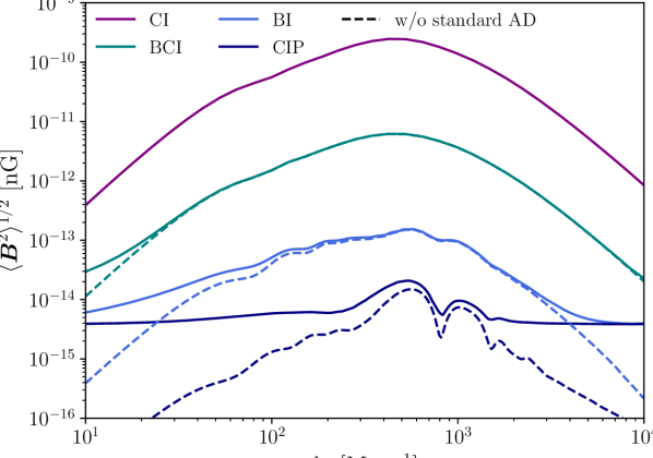
One would naively think that the magnetic field from isocurvature perturbations should be roughly a factor of larger than that sourced by standard adiabatic perturbations. However, this is not the case as the growth rate of perturbations is in general much slower for isocurvature perturbations than for adiabatic perturbations (see Fig. 1), since CDM perturbations are not boosted by the gravitational potential sourced by photon perturbations in the radiation-dominated era.
Let us note that CIPs were first considered as a source of magnetic fields through the Biermann-battery mechanism in Ref. Flitter et al. (2023), whose authors considered CIPs with power-law primordial power spectra. Our treatment is much more detailed in several respects, leading to up to one order of magnitude difference with the results of Ref. Flitter et al. (2023) with equal assumptions for the CIP primordial power spectrum. We discuss the differences between our work and theirs in Appendix. C.
V Conclusion
In this paper we make the most accurate calculation to date of the magnetic field produced by a variety of primordial perturbations through the Biermann-battery mechanism. To do so, we consistently solve for the evolution of small-scale perturbations in electron density and baryon gas temperature, including the effect of large-scale relative velocity between CDM and baryon.
We first calculate the magnetic field produced solely from standard, nearly-scale invariant primordial adiabatic perturbations. Our results update and supersede those of the pioneering work NN13 Naoz and Narayan (NN13), as we correctly compute the electron density perturbation, and account for the full angular dependence of the magnetic field power spectrum on relative velocities. We show that the resulting “standard” magnetic field can reach an rms of a few times nG at , with maximal fluctuations on comoving scales Mpc-1. This magnetic field can serve as a seed field to be later amplified by dynamo processes, possibly explaining the magnetic fields present in galaxies and galaxy clusters today Durrer and Neronov (2013).
In addition, using the fact that the main contribution to magnetic field comes from perturbations on very small scales Mpc-1, we argue that measuring magnetic fields can be a useful probe for initial conditions of the Universe on such small scales. We first consider enhanced small-scale primordial adiabatic perturbations, and show that they can source magnetic fields as large as nG without violating current CMB spectral distortion constraints. We similarly compute the magnetic field sourced by a variety of small-scale isocurvature perturbations (baryon, CDM, joint baryon and CDM, and compensated baryon-CDM isocurvature perturbations). We find that such non-standard perturbations could generate magnetic fields as large as nG at cosmic dawn, depending on the specific type of isocurvature mode, without violating current BBN and perturbed recombination constraints. While these are extremely weak magnetic fields, below current detection capabilities, they may still be a useful observable to consider in the future, as they could provide a new window into the poorly constrained small-scale initial conditions of the Universe.
Acknowledgements
We thank Marc Kamionkowski for useful conversations and encouragements, Smadar Naoz for providing details and data relevant to her work on the topic, and Jordan Flitter for providing his results for a comparison with our work, as well as sending detailed comments about this manuscript. N. L. is supported by the Center for Cosmology and Particle Physics at New York University through the James Arthur Graduate Associate Fellowship. Y. A.-H. is a CIFAR-Azrieli Global Scholar and acknowledges support from the Canadian Institute for Advanced Research (CIFAR), and is grateful for being hosted by the USC departement of physics and astronomy while on sabbatical. This work was supported in part through the NYU IT High Performance Computing resources, services, and staff expertise.
Appendix A Derivation of the Biermann-battery mechanism
In this appendix we provide a pedagogical derivation of the Biermann-battery mechanism, in the cosmological context. For simplicity we do not account for cosmic expansion in this derivation (alternatively, it can be thought of as a derivation in a locally-inertial coordinate system), and restore dependence on scale factors in the final result. We work in units where .
A.1 Electron-proton slip and current density
We consider free electrons and free protons as two distinct ideal fluids (a more rigorous approach would use kinetic theory and follow their distribution functions). For each fluid , we denote by its number density, its mass density, its velocity, its temperature and its pressure. Assuming helium is fully neutral, all of these fields are nearly identical for electrons and protons, except for their mass densities, .
In the presence of an electric and magnetic field, the momentum equations satisfied by each fluid are
| (27) | |||||
| (28) | |||||
where is the elementary charge, and we neglected photon drag. Aside from the obvious gravitational, pressure and electromagnetic forces, the last term, proportional to the relative velocity between electrons and protons, represents the drag force arising from frequent Coulomb interactions between the two species – it is this term which, in practice, forces electrons and protons to be behave very nearly as a single fluid. Subtracting the two equations, and only keeping terms at lowest order in , we obtain an equation for the “slip”, i.e. the velocity difference between the two species:
| (29) |
Let us now estimate : it is of the order of the rate of interactions between electrons and protons, namely , where is the Coulomb interaction cross section and is the microscopic (in contrast with the macroscopic averages ) relative velocity of electrons and protons – for completeness, exact expressions for the momentum-exchange rate can be found in Refs. Ali-Haïmoud (2019); Ali-Haïmoud et al. (2023). The Coulomb scattering cross section is approximately , where is the Thomson cross section. Since microscopic relative velocities between electrons and protons are dominated by the electrons’ thermal velocities, we find
| (30) |
We may estimate the ratio of this rate relative to the Hubble rate by noting that the Thomson scattering rate becomes comparable to the Hubble rate around redshift , at which point . Hence, we find (assuming during matter domination, and with ),
| (31) |
The electron temperature is approximately
| (32) |
where the transition at corresponds to thermal decoupling from photons. Therefore, we find, at ,
| (33) |
where we have normalized to its freeze-out abundance. We thus see that, at all relevant times, , implying that electrons and protons are tightly coupled. This allows us to estimate the slip relative velocity by solving Eq. (29) in the quasi-steady-state approximation:
| (34) |
This slip is an important quantity as it allows us to determine the electric current density . We thus have found
| (35) |
A.2 Combining with Maxwell’s equations
We now combine Eq. (35) with Maxwell’s equations. Given a current density , the magnetic field satisfies the forced wave equation
| (36) |
When considering scales much smaller than the Hubble radius, one may neglect the first term relative to the second one in the right-hand-side of Eq. (36). Taking the curl of Eq. (35) and using Maxwell-Faraday equation (and neglecting small fluctuations of the prefactor in front of ), we obtain
| (37) |
where we have defined a characteristic lengthscale
| (38) |
where we used Eq. (30) and . Inserting Eq. (32), we thus obtain, for
| (39) |
For fluctuations on a comoving scale , the ratio of the term proportional to to the first term in Eq. (36) is of order
| (40) | |||||
Therefore, we see that, for any cosmological scales of interest, the term proportional to may be safely neglected in Eq. (37). If we restrict ourselves to small perturbations in the electron density, we may moreover neglect the term . We have thus found
| (41) |
With , and , , we find
| (42) |
Re-expressing proper gradients in terms of comoving gradients, and accounting for the dilution of magnetic fields by due to cosmological expansion, we recover Eq. (6).
Appendix B Numerical implementation details
In this appendix we detail our numerical implementation of the magnetic field power spectrum.
We first store the transfer functions of electron density perturbations and baryon gas temperature perturbations in tables. We note that, for large relative velocities or small scales, all perturbations are proportional to the rapidly-oscillating component , with phase
| (43) | |||||
where . Instead of tabulating the rapidly-oscillating small-scale transfer functions themselves, we thus tabulate their slow-varying parts
| (44) |
This allows us to get accurate interpolation results with a coarser table. For small-scale modes, we store the slow-varying parts for 1,300 wavenumbers , 200 values of , and 300 redshift points in logarithmically spaced in scale factor (or equivalently in ). For large-scale modes, we store transfer functions only with for 450 wavenumbers and 1,000 redshifts . When needed, we interpolate these tables using Python Scipy cubic spline interpolator.
We compute the time integral in [Eq. (9)], using the trapezoidal rule with the 300 logarithmically-spaced redshifts in at which we store the transfer functions at high ’s. This avoids having to do 3-dimensional interpolation: we only interpolate over and for each given redshift grid-point. In principle, this time integral should be extended to (or ), but we checked that it is in fact already well converged when only including , since the integral is dominated by late times.
For given values of and , we compute the 3-dimensional -integral of Eq. (12) as follows. We define the -axis to be aligned with the vector , and let be on - plane without loss of generality. We then perform the integral in spherical polar coordinates , noting that the symmetry of the problem implies . We then perform 21-point Gaussian-Quadrature integration for . We rewrite the polar angle integral as , where we define , and then perform 21-point Gaussian Quadrature integration for . This is to better handle a divergence which happens because the integrand scales as when . Given a set of two angular variables, we integrate over from to using the 1-dimensional integrator in Python Scipy package (scipy.integration.quad). Finally, we compute the 2-dimensional angular integral by trapezoidal rule over sampled points of and .
Appendix C Comparison with Flitter et al. 2023 Flitter et al. (2023)
In this appendix, we review the assumptions taken in Ref. Flitter et al. (2023) (hereafter F+23) to compute the magnetic field generated by CIPs, and contrast them with our detailed calculation.
On scales much larger than the baryon Jeans scale, baryon and CDM perturbations are known to remain constant in time for CIP initial conditions. Motivated by this result, F+23 assume a strictly constant baryon perturbation for all scales Mpc-1, and compute the resulting late-time free-electron density perturbation, finding . In contrast, we compute the full time evolution of the free-electron density perturbation, as a function of scale, and find that it significantly differs from (and can be significantly larger than) this constant value even at scales Mpc-1, as can be seen in Fig. 1.
In addition, F+23 neglect the gas temperature fluctuations sourced by CIP initial conditions, hence only account for the cross term in the magnetic field source. This assumption is self-consistent with their assumption of constant , implying , which thus cancels the main source of gas temperature fluctuations in Eq. (1). In contrast, we self-consistently account for CIP-sourced gas temperature fluctuations, which are in fact comparable to free-electron density perturbations even for scales significantly larger than the Jeans scale (see Fig. 1). We thus effectively account for two more terms in the magnetic field source: and .
Moreover, F+23 assume that the AD-sourced gas temperature fluctuations strictly follow the baryon density fluctuations, . In turn, baryon density fluctuations are assumed to precisely match the total matter density fluctuation up to a constant Jeans scale Mpc-1, and to be suppressed by a factor for smaller scales Naoz and Barkana (2005); Naoz et al. (2011), i.e. modeled as . F+23 then model the matter power spectrum using class at large scales, extended to small scales () by the Bardeen-Bond-Kaiser-Szalay fitting function Bardeen et al. (1986) with baryon corrections of Ref. Sugiyama (1995). In contrast, we self-consistently compute the electron density and gas temperature perturbations for AD initial conditions, without imposing a constant bias with respect to density fluctuations nor any approximate cutoff at the Jeans scale.
Last but not least, F+23 do not account for relative velocities between CDM and baryons. Interestingly, these supersonic relative motions break the exact cancellation of the gravitational potential, thus allowing density perturbations to grow on scales larger than the baryon Jeans scale. This effect is thus qualitatively the opposite from what happens for adiabatic perturbations Tseliakhovich and Hirata (2010). However, it does not necessarily lead to an overall increase of the magnetic field power, since it pushes gas temperature fluctuations closer to the adiabatic limit , and makes the ratio closer to being scale-invariant, i.e. “aligns” more the gradients of gas temperature and electron density fluctuations.
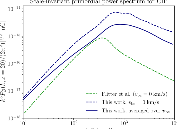
As a concrete example, we consider a scale-invariant primordial power spectrum for CIPs, , corresponding to the spectral index case in F+23. In that case the upper limit on is dominated by large-scale CMB-anisotropy constraint, which with our convention333Ref. Smith et al. (2017) define instead of our is Smith et al. (2017).
We see in Fig. 6 that the magnetic field from our calculations without any approximations is an order of magnitude larger than the result of F+23 at . Note that the difference would have even been larger had we not included relative velocities, which lower the rms magnetic field by a factor of . Also note that, while the observable magnetic field also includes contributions from standard adiabatic modes alone [shown to be in Fig. 2], for a fair comparison, in Fig. 6 we only include contributions from CIPs, sourced by , , and .
References
- Vallée (2004) J. P. Vallée, New Astron. Rev. 48, 763 (2004).
- Neronov and Vovk (2010) A. Neronov and I. Vovk, Science 328, 73 (2010), arXiv:1006.3504 [astro-ph.HE] .
- Beck (2012) R. Beck, Space Science Reviews 166, 215 (2012).
- Durrer and Neronov (2013) R. Durrer and A. Neronov, Astron. Astrophys. Rev. 21, 62 (2013), arXiv:1303.7121 [astro-ph.CO] .
- Davis et al. (1999) A.-C. Davis, M. Lilley, and O. Tornkvist, Phys. Rev. D 60, 021301 (1999), arXiv:astro-ph/9904022 .
- Biermann (1950) L. Biermann, Zeitschrift Naturforschung Teil A 5, 65 (1950).
- Naoz and Narayan (NN13) S. Naoz and R. Narayan (NN13), Phys. Rev. Lett. 111, 051303 (2013), arXiv:1304.5792 [astro-ph.CO] .
- Tseliakhovich and Hirata (2010) D. Tseliakhovich and C. Hirata, Phys. Rev. D 82, 083520 (2010), arXiv:1005.2416 [astro-ph.CO] .
- Flitter et al. (2023) J. Flitter, C. Creque-Sarbinowski, M. Kamionkowski, and L. Dai, Phys. Rev. D 107, 103536 (2023), arXiv:2304.03299 [astro-ph.CO] .
- Aghanim et al. (2020) N. Aghanim et al. (Planck), Astron. Astrophys. 641, A6 (2020), arXiv:1807.06209 [astro-ph.CO] .
- Chluba and Grin (2013) J. Chluba and D. Grin, Mon. Not. Roy. Astron. Soc. 434, 1619 (2013), arXiv:1304.4596 [astro-ph.CO] .
- Venumadhav et al. (2017) T. Venumadhav, A. Oklopcic, V. Gluscevic, A. Mishra, and C. M. Hirata, Phys. Rev. D 95, 083010 (2017), arXiv:1410.2250 [astro-ph.CO] .
- Gluscevic et al. (2017) V. Gluscevic, T. Venumadhav, X. Fang, C. Hirata, A. Oklopcic, and A. Mishra, Phys. Rev. D 95, 083011 (2017), arXiv:1604.06327 [astro-ph.CO] .
- Blas et al. (2011) D. Blas, J. Lesgourgues, and T. Tram, JCAP 07, 034 (2011), arXiv:1104.2933 [astro-ph.CO] .
- Ali-Haimoud and Hirata (2010) Y. Ali-Haimoud and C. M. Hirata, Phys. Rev. D 82, 063521 (2010), arXiv:1006.1355 [astro-ph.CO] .
- Ali-Haimoud and Hirata (2011) Y. Ali-Haimoud and C. M. Hirata, Phys. Rev. D 83, 043513 (2011), arXiv:1011.3758 [astro-ph.CO] .
- Lee and Ali-Haïmoud (2020) N. Lee and Y. Ali-Haïmoud, Phys. Rev. D 102, 083517 (2020), arXiv:2007.14114 [astro-ph.CO] .
- Lee and Ali-Haïmoud (2021) N. Lee and Y. Ali-Haïmoud, Phys. Rev. D 104, 103509 (2021), arXiv:2108.07798 [astro-ph.CO] .
- Naoz and Barkana (2005) S. Naoz and R. Barkana, Mon. Not. Roy. Astron. Soc. 362, 1047 (2005), arXiv:astro-ph/0503196 .
- Lewis (2007) A. Lewis, Phys. Rev. D 76, 063001 (2007), arXiv:0707.2727 [astro-ph] .
- Senatore et al. (2009) L. Senatore, S. Tassev, and M. Zaldarriaga, JCAP 08, 031 (2009), arXiv:0812.3652 [astro-ph] .
- Ali-Haïmoud et al. (2014) Y. Ali-Haïmoud, P. D. Meerburg, and S. Yuan, Phys. Rev. D 89, 083506 (2014), arXiv:1312.4948 [astro-ph.CO] .
- Peebles (1968) P. J. E. Peebles, Astrophys. J. 153, 1 (1968).
- Venumadhav and Hirata (2015) T. Venumadhav and C. Hirata, Physical Review D 91 (2015), 10.1103/physrevd.91.123009.
- Papanikolaou and Gourgouliatos (2023) T. Papanikolaou and K. N. Gourgouliatos, Phys. Rev. D 107, 103532 (2023), arXiv:2301.10045 [astro-ph.CO] .
- Chluba et al. (2012) J. Chluba, A. L. Erickcek, and I. Ben-Dayan, Astrophys. J. 758, 76 (2012), arXiv:1203.2681 [astro-ph.CO] .
- Fixsen et al. (1996) D. J. Fixsen, E. S. Cheng, J. M. Gales, J. C. Mather, R. A. Shafer, and E. L. Wright, Astrophys. J. 473, 576 (1996), arXiv:astro-ph/9605054 [astro-ph] .
- Inomata et al. (2018) K. Inomata, M. Kawasaki, A. Kusenko, and L. Yang, JCAP 12, 003 (2018), arXiv:1806.00123 [astro-ph.CO] .
- Ali-Haïmoud (2019) Y. Ali-Haïmoud, Physical Review D 99 (2019), 10.1103/physrevd.99.023523.
- Ali-Haïmoud et al. (2023) Y. Ali-Haïmoud, S. S. Gandhi, and T. L. Smith, (2023), arXiv:2312.08497 [astro-ph.CO] .
- Naoz et al. (2011) S. Naoz, N. Yoshida, and R. Barkana, Mon. Not. Roy. Astron. Soc. 416, 232 (2011), arXiv:1009.0945 [astro-ph.CO] .
- Bardeen et al. (1986) J. M. Bardeen, J. R. Bond, N. Kaiser, and A. S. Szalay, Astrophys. J. 304, 15 (1986).
- Sugiyama (1995) N. Sugiyama, Astrophys. J. Suppl. 100, 281 (1995), arXiv:astro-ph/9412025 .
- Smith et al. (2017) T. L. Smith, J. B. Muñoz, R. Smith, K. Yee, and D. Grin, Phys. Rev. D 96, 083508 (2017), arXiv:1704.03461 [astro-ph.CO] .