FTPI-MINN-24-05, UMN-TH-4314/24
Lie-algebraic Kähler sigma models
with the U(1) isotropy
Chao-Hsiang Sheua and Mikhail Shifmana,b
aDepartment of Physics,
University of Minnesota,
Minneapolis, MN 55455
and
bWilliam I. Fine Theoretical Physics Institute,
University of Minnesota,
Minneapolis, MN 55455
Abstract
We discuss various questions which emerge in connection with the Lie-algebraic deformation of sigma model in two dimensions. First we supersymmetrize the original model endowing it with the minimal and extended supersymmetries. Then we derive the general hypercurrent anomaly in the both cases. In the latter case this anomaly is one-loop but is somewhat different from the standard expressions one can find in the literature because the target manifold is non-symmetric. We also show how to introduce the twisted masses and the term, and study the BPS equation for instantons, in particular the value of the topological charge. Then we demonstrate that the second loop in the function of the non-supersymmetric Lie-algebraic sigma model is due to an infrared effect. To this end we use a supersymmetric regularization. We also conjecture that the above statement is valid for higher loops too, similar to the parallel phenomenon in four-dimensional super-Yang-Mills. In the second part of the paper we develop a special dimensional reduction – namely, starting from the two-dimensional Lie-algebraic model we arrive at a quasi-exactly solvable quantum-mechanical problem of the Lamé type.
1 Introduction
In this paper we continue the studies of one(complex)-dimensional sigma models on Kählerian target spaces which generalize the model in a Lie-algebraic way [1, 2, 3]. For practical applications in baby Skyrmions this model is usually formulated in the from
| (1.1) |
where the coupling becomes a function of , the third component of the isovector ,
| (1.2) |
Moreover, is a numerical parameter defined below in Eq. (1.5). At we return to the Heisenberg O(3) model. With the round metric is deformed.
For theoretical applications in two dimensions (2D) it is more convenient to use the geometric representation,
| (1.3) |
where is a generalization of the Fubini-Study metric,111The equality can always be achieved by rescaling the fields .
| (1.4) | |||||
| (1.5) |
If the metric (1.4) is the standard Fubini-Study metric. In what follows we will use a simplified notation,
One can consider another deformation of this model, by the so-called twisted mass term [4, 5]. Then, Eq. (1.3) takes the form
| (1.6) |
In temrs of representation (1.1) we then have
| (1.7) |
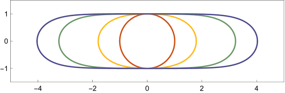
Both deformations (i.e. the metric deformation and a “potential” deformation ) destroy O(3) invariance of the target space and introduce a dependence on the orientation of with respect to the third axis in the isospace, see Fig. 1.
Perturbation theory in the model at hand have been studied in [1, 2] in the framework of the so called first-order formalism related to an operator product expansion (OPE), see the list of references in [1, 2]. The following phenomenon have been observed there.
At one loop OPE for certain chiral currents have the form
| (1.8) |
where are the algebra structure constants. The above expression fully reveals the Lie-algebraic structure of (1.4). However, a straightforward calculation of the second loop produces a term
| (1.9) |
where are Killing vectors. The above structure is obviously non-geometric. However, one can show that with a proper regularization within the first-order formalism the partial derivatives in (1.9) are replaced by covariant derivatives, and the required “geometricity” is recovered. In Ref. [2] the regularization method was based on supersymmetry despite the fact that the calculated function was that of the non-supersymmetric model (1.3). In [1] the following hypothesis was formulated: In (non-supersymmetric) Kählerian sigma models, an anomaly is present in the calculation of the second and higher loops. In [2] the validity of the hypothesis was verified in the second loop.
In this paper we reveal an infrared anomaly in the second -function coefficient. We use the standard perturbation theory and standard two-loop Feynman graphs. Our derivation is based on supersymmetry; however, the strategy is different from that in [2]. Our analysis has close parallels with the holonomy anomaly in supersymmetric Yang-Mills (SYM) theory [6] and two-dimemsional sigma models [7, 8]. Just like in the latter case it is likely that the anomalous effect detected in non-supersymmetric Kählerian sigma models can be reformulated as a subtlety in the measure in the corresponding path integral [9].
Our work consist of several parts. First, we supersymmetrize the model (1.3), (1.4), presenting both and versions. Section 2.1.3 is devoted to the study of the hypercurrents in and versions of the model. The standard expressions known in the literature have to be modified to take into account the non-symmetric nature of the target space. Then, in Secs. 2.2 and 2.3 we introduce the twisted mass and the angle.
In Sec. 3 we calculate the two-loop function coefficient in the non-supersymmetric sigma model by virtue of a supersymmetric regularization. Our calculation is transparent and demonstrates the role of the infrared contribution. Section 4 is devoted to an interesting aspect of reducing the two-dimensional model under consideration to a Lie-algebraic quantum-mechanical model [10, 11] presenting the so-called Lamé problem [12]. Under certain values of quantized free parameters it becomes quasi-exactly solvable, and, moreover, exhibits duality in the non-supersymmetric case.
2 Extending the deformed model
In this section, we elaborate on supersymmetric extensions of the deformed model, incorporating twisted masses and a topological term in a consistent manner. Applications of the present construction to the analysis of functions and the reduced quantum mechanical model can be found in Sec. 3 and 4, respectively.
2.1 and supersymmetrization
2.1.1
We start with a brief review of the general construction of two-dimensional and sigma models. The target space of the model under consideration is a one (complex) dimensional manifold; it is Kählerian and admits structure [13]. Since the basics of the model can be found in standard textbooks, we just quote the results and remind the relevant geometric data. Suppose the target space is parametrized by the complex coordinates and . By promoting the scalar field to the corresponding superfields, , and integrating out the Grassmann coordinates, one finds the component formulation (see for example [14, 15]), namely,
| (2.1) |
where is a Dirac fermion,
| (2.2) |
and
| (2.3) |
is the Christoffel symbol. The essential geometric data (in addition to Eq. (1.4)) are
| (2.4a) | ||||
| (2.4b) | ||||
in which is the scalar curvature,
| (2.5) |
2.1.2
As for the formulation, we limit our discussion to the so-called minimal model [7]. Following the same lines as in [16, 8, 17], we introduce an chiral superfield which, in terms of component fields, takes the form
| (2.6) |
where and are the Grassmann coordinates. The supersymmetric transformation of is
| (2.7) |
The Lagrangian can be written as
| (2.8) |
Note that is the first derivative of the Kähler potential,222The explicit form of the Kähler potential of the deformed model is given in [3].
| (2.9) |
By construction, Eq. (2.1.2) is invariant. In contrast to the undeformed model, there is no nonlinear transformation of corresponding to the global rotations other than the which can be straightforwardly seen in the above formulation.
As a side remark, we note that the supersymmetry can be recovered from Eq. (2.1.2) by introduced another superfield ,
| (2.10) |
obeying the transformation
| (2.11) |
The corresponding Lagrangian is
| (2.12) |
where is the metric obtained by promoting to , respectively, in (2.4a). Note that we have integrated out the auxiliary field. One can then see that the combination of (2.1.2) and (2.1.2) leads to Eq. (2.1). The enhancement of the supersymmetry from to was first demonstrated in [18] for the undeformed case.
2.1.3 Hypercurrent multiplet
In the following, we analyze the hypercurrent multiplet (see [5, 19, 20, 21] for review and examples) of the deformed model. Our discussion on the case of will run parallel to that of [5]. This supermultiplet contains a -current , a supercurrent , and the energy-momentum tensor ,
| (2.13) |
where the matrices are defined as
| (2.14) |
Here the Grassmannian coordinate has two complex components in contrast to the case of which has only one relevant Grassmannian coordinate. The lowest component in the hypercurrent is the vector U(1) current. Although classically is algebraically related to the axial current discussed in Sec. 2.3) at the quantum level they are different – the axial current has an anomaly.333In fact, there are three independently conserved U(1) currents in this model. The first is the axial current presented in Eq. (2.35). It is generated by the transformation (2.36), conserved at the classical level and acquires a one-loop anomaly in . The second conserved current is purely bosonic, it is generated by the transformation and . Needless to say, it is anomaly-free. The third is purely fermionic vector current, also anomaly-free. In the spinorial notation, it takes the form
| (2.15) |
where and are superderivatives and and are the chiral superfields with the lowest components and , respectively. At the classical level, the spinorial components and are conserved, namely,
| (2.16) |
In , only two diagonal components of are relevant.
Quantum mechanically, the hypercurrent expressions in (2.16) are anomalous The anomaly is exhausted by the one-loop effect. For the anomaly equations were derived in [5]. In our deformed model the anomaly in the right-hand side takes the form
| (2.17) |
Note the emergence of the scalar curvature on the right-hand side.
The coefficient in (2.17) can be verified through the scale anomaly of the energy-momentum tensor i.e. the anomaly in [5, 22],
| (2.18a) | ||||
| (2.18b) | ||||
Note that the hypermultiplet falls in the class of the -multiplets in [21] since . In fact, Eq. (2.17) can be recast in the standard form of the hypercurrent multiplet proposed in [20, 21]. Namely,444For a general model, the anomalies of the hypercurrent take the form (2.19) This issue was previously discussed in [20] for the case of the symmetric Kähler manifolds. Since in our deformed model the target space is non-symmetric, the expression in the right-hand side of (2.19) is somewhat different from that in [20].
| (2.20) |
for which we use the fact that only the twisted chiral (antichiral) part of contributes in the first (second) equations in (2.17).
*****
The hypercurrent for the model was discussed in [7, 8]. Taking into account our Lie-algebraic extension we arrive at the classical expressions
| (2.21a) | ||||
| (2.21b) | ||||
where and stand for two components in the hypercurrent in the model, and is the superfield defined in Sect. 2.1.2. In the superspace, the reduced superderivatives are
| (2.22) |
Here the lowest component of is the chiral current and is not conserved as the quantum corrections are taken into account. Also, the bosonic component of is the part of the energy-momoentum tensor, .
In general, like in the case, the hypercurrent (2.21) is conserved classically and becomes anomalous due to one-loop corrections. In other words, the general anomaly equations turn out to be
| (2.23) |
where encodes the anomalous part of two real supermultiplets and . Note that the coefficient of Eq. (2.23) can be fixed by the anomalous chiral current in parallel to the consideration of the axial current in Appendix B,
| (2.24) |
where the prefactor indicates the number of the fermion zero modes in the instanton background, which is half of the number in theory, see also (2.37).
Important warning: in the case, the function is not exhausted by one loop, see Sect. 3. Therefore, the one-loop anomaly expression given in (2.23) should be understood as an operator expressions subject to further infrared multi-loop corrections, just in the same way as in super-Yang-Mills (see [6] and Secs. 10.16.1-10.16.4 in [23]). In our problem, the latter conjecture is not yet proven.
2.2 Adding twisted masses
As observed in [4, 24, 25, 26], one can introduce the twisted mass parameter consistent with the underlying supersymmetries in the presence of the isometry of the system. That is, the infinitesimal transformations read
| (2.25) |
where is the variable parametrizing the isometry. Notice that for the deformed model, such an isometry can be summarized by the Killing potential ,
| (2.26) |
generating the Killing vectors, namely,
| (2.27) |
Here the Killing potential is defined up to an additive constant.
One can then introduce a constant auxiliary vector multiplet parametrized by the twisted masses, and , to modify the invariant combination in the associated Kähler potential as . In the following, we directly quote the resulting Lagrangian. The interested readers can find a concise review in Sec. 2 of [5]. The deformed model with the twisted masses is formulated as follows 555Generally speaking, for a sigma model with a complex target space with the Killing vectors for the isometries the associated Lagrangian takes the form where is the covariant derivative on the target space.
| (2.28) |
where is the covariant derivative
| (2.29) |
and
| (2.30) |
Similarly, one can introduce the twisted mass for the model by replacing the aforementioned constant auxiliary vector multiplet with a one. As a result, the model with twisted mass takes the form
| (2.31) |
where is real in the case.
2.3 The term
The term can be added in a straightforward manner [5, 22],
| (2.32) |
Note that the theta term is topological and invariant under translation since the topological charge defined as
| (2.33) |
In particular, for the (anti-)instanton solution. For completeness, the theta term can also be expressed as a total derivative
| (2.34) |
This also indicates that (2.33) saturates at the small field configuration.
The theta term (2.32) can be further utilized to detect the number of fermion zero modes and then the number of the bosonic zero modes via supersymmetry. To this end, let us consider the divergence of the axial current
| (2.35) |
generated by the transformation
| (2.36) |
where is the variable parametrizing the transformation. Classically, is conserved, but it becomes anomalous as the quantum effects are taken into account. Namely, in ,
| (2.37) |
implying the number of the fermion zero modes is four and therefore the same for the bosonic sector through supersymmetry. See Appendix B for further detail. Comparing with Eq. (2.32), one sees that under the axial rotation (2.36), which breaks into .
Furthermore, it is worth pointing out how the instanton action is related to the topological charge defined in (2.33). According to the standard BPS argument, the action satisfies
| (2.38) |
where is the topological charge. The action saturates the BPS bound for the instanton configuration. In the non-degenerate case (i.e. ), the overall coefficient in front of in (2.3) is
| (2.39) |
as was previously derived in [3]. The expression can be obtained by further taking the limit.
3 Analysis of the two-loop beta function
3.1 The two-loop beta function of the bosonic model from supersymmetry
We will start from the universal fact that the second (and all higher) coefficients of two-dimensional sigma models vanish [27, 28], see also [29, 30] for recent discussions.666 In the mid-1980s this fact was questioned by Grisaru, van de Ven and Zanon [31] who analyzed the functions in two-dimensional Kähler models up to four loops. In the case of the Ricci-flat manifolds they arrived at the conclusion that there is a non-vanishing contribution to the function cubic in the Riemann curvature of the target space at the fourth loop. This result is in the direct contradiction with those reported in [32, 33]. The class of models we study is not Ricci-flat. Morever, in Sec. 3.3 we will argue that the result [31] cannot be applied to the model under discussion. Our argument is based on the Dorey’s exact solution [26] for the mass spectrum in à la Seiberg-Witten type [34, 35]. In supersymmetric sigma models the two-loop contributions to the function can be separated into the (purely) bosonic and fermionic parts. In other words,
| (3.1) |
which implies, in turn, that the purely bosonic component can be extracted from the fermionic part (which is much more amenable for loop calculations),
| (3.2) |
Note that is identical to the beta function of the non-supersymmetric case.
To confirm the previous assertion, let us apply the background field method. It suffices to consider the two-loop fermionic diagram in Fig. 2 – the only non-trivial diagram with the requred logarithmic divergence.

Here are the external legs, and , , and their complex conjugates are the quantum scalar field and fermions, respectively. To proceed, we consider the background expansion via the Kähler coordinates [36, 37]. The only relevant interactions in Fig. 2 are the 3-vertices, namely,
| (3.3) |
where . Therefore, the two-loop fermion correction to the Lagrangian (2.1) is
| (3.4) |
where the ellipses stand for non-logarithmic divergences and in dimensional regularization. In accordance with the renormalization group equation (see e.g. [38, 27]), we then have
| (3.5) |
Note that to get the second equality, the first equation in (2.4b) is used.
Now, invoking (3.2) we arrive at
| (3.6) |
which matches with the general formula in the purely bosonic model [38],
| (3.7) |
In the present case, all the Greek indices are 1. As a consistent check, taking the limit in (1.5) we recover the result 777This calculation for in was first presented in [23], page 265, see also subsection 3.1.1.
| (3.8) |
As explained in detail in [23] on pages 674-676, the calculation of the graph in Fig. 2 becomes transparent if we first deal with the fermion loop keeping fixed the momentum flowing through the dashed (bosonic) line. As is clear from Eq. (3.3) the fermion loop is exactly the same as in the two-dimensional Schwinger model. It has no logarithms and is saturated in the infrared. Including the bosonic loop provides us with the first power of . This is exactly what is expected in the two-loop graph for the function. The Schwinger “anomaly” is crucial.
3.1.1 Verification around the origin
If we limit ourselves to the vicinity of the origin in the target space and forget for a short while about the target space invariance, the proof of our assertion can be greatly simplified. Indeed, because the overall structure of the field dependence is constrained by the target space geometry of the deformed model, we can accept that the second coefficient of the beta function in the bosonic model takes the form
| (3.9) |
Plugging the explicit expression for the geometric data given in Eq. (2.4), one sees that
| (3.10) |
for . In the same approximation, the leading terms in the Lagrangian are
| (3.11) |
Then, considering the same two-loop diagram in Fig. 2, we obtain the two-loop Lagrangian
| (3.12) |
where and are the ultraviolet and infrared cutoffs, respectively. The constant turns out to be
| (3.13) |
consistent with the covariant derivation given in (3.5).
3.1.2 The two-loop beta function of extension
Based on the result of Eq. (3.5), the second coefficient of the beta function for minimal sigma models with a one-complex-dimensional target space can be readily identified. To see that this is the case, note that the fermion sector in models consists of two Weyl fermions (one left-handed fermion and one right-handed) while in models, there exists only one Weyl fermion. This indicates that the contribution from fermions at the two-loop level is half of Eq. (3.5) in the case. Consequently, combining with the bosonic contribution, we obtain the second coefficient of the beta function that
| (3.14) |
Going through the same process around (3.8), one would see the second coefficient of the model
| (3.15) |
which was first derived in [7] through the superfield calculation.
3.2 Comparison with the first-order formalism
Our results (3.6) for the bosonic model coincides with that obtained in [2] by virtue of the first-order formalism. The regularization procedure used in [2] was as follows. We start from the theory. In first-order formalism it is obvious that all loops in beyond the first loop vanish – there is no anomaly and holomorphy is preserved. Then we endow the fermion field with a mass term and compute the function coefficients with large but fixed value . In the limit we discover that some “extra” terms do not vanish. It is just these extra terms which are responsible for the transition from in (1.9) to where stands for the covariant derivative. This procedure can be viewed as an ultraviolet derivation of the anomaly.
3.3 Comment on the literature
We started Sec. 3.1 from the statement that “the second (and all higher) coefficients of two-dimensional sigma models vanish.” In this subsection we will discuss this statement in more detail. A series of papers on this subject was published in [32, 33, 39] in the early 1980s. Then this issue was revisited 1985-86, approximately simultaneously with the publication [31].
The authors of [31] state the opposite – that the functions in two-dimensional Ricci flat Kähler models have a non-vanishing contribution at four loops cubic in the Riemann curvature of the target space, see their Eq. (5.16).
The class of Lie-algebraic models we are interested in (it includes, in particular models) is not not Ricci-flat. In 37 years that elapsed since the publication of Grisaru et. al. a significant progress happened in understanding both perturbation theory and exact solutions in models (and their extensions) and, in “parallel” to them, exact solutions in Yang-Mills theories with various degrees of supersymmetry.
If supersymmetry is minimal, the functions are indeed multi-loop, but are exactly calculable. For supersymmetry the perturbative functions are exhausted by the first loop. This is seen from the analysis of the holomorphy properties with regards to the complexified coupling constant
in super-Yang-Mills and
in 2D models (see below). Moreover, this statement is confirmed by the exact solutions.
The exact solution for the mass spectrum of the Seiberg-Witten super-Yang-Mills [34, 35] (say, for SU(2), parametrized by a single modular invariant , being expanded in the ratio exhibits the first order in plus all powers of
| (3.16) |
The power terms of the expansion (3.16) do not contain logarithms and come from instantons (this series can be – and in fact, has been – obtained by using the Nekrasov localization [40]).
Next, in 1998 Dorey published a paper [26] in which he obtained the exact solution à la Seiberg-Witten for the models with twisted masses (in there is only one twisted mass parameter). Dorey’s method repeats the Seiberg-Witten’s analysis [34, 35] in Yang-Mills step by step.
If one replaces the twisted mass of model by the modular parameters of the Seiberg-Witten derivation in Yang-Mills, then the formula for the spectrum in Yang-Mills in four dimensions is exactly the same as the Dorey’s formulae in in two dimensions (see Eqs. (112) in the general case and (117) for a particular case of in [26].)
Dorey’s observation [26] can be summarized as follows:
The mass spectrum on the Coulomb branch ( where is the Fayet-Iliopoulos term) of the Seiberg-Witten theory, with unconfined ‘t Hooft-Polyakov-like monopoles and dyons coincides with that of models emerging on the vortex string [41, 42] in the Higgs phase (i.e. ). In [41] it was proved that the central charges cannot depend on the non-holomorphic parameter in the BPS sector. This established a one-to-one correspondence between the mass spectra of the two seemingly different theories. They prove to be identical in the BPS sectors, hence, - correspondence.
Dorey’s formula for the BPS mass spectrum depends on the ratio , where is the twisted mass, and is the scale parameter of the theory, obtained through the dimensional transmutation (as in any asymptotically free theory). Let us assume that this parameter is large and expand the Dorey’s exact solution in the ratio . In parallel with Yang-Mills the Dorey expansion contains the first order in plus powers of
where comes from , with nothing else.
We emphasize, that the perturbative term is is unique. There are no terms or , etc. in the expansion of the exact formula. Since the masses are physically observable, their expression must be consistent with the function. This can only happen if the perturbative function is purely one-loop in the class of models under consideration.
Just for completeness, let us mention that in minimal supersymmetries (such as Yang-Mills or ) the functions contain all loops. However, if it were not for holomorphic anomaly [43, 44], all coefficients, starting from the two-loop coefficient would vanish – only the one-loop coefficient would survive. The break down of holomorphy is an infrared effect [43, 44], which is well understood. This is best illustrated by the instanton formula (IR is automatically regularized in the instantion background). Its general form valid both for super-Yang-Mills and (without matter fields) is as follows,
| (3.17) |
where and are the numbers of the bosonic and fermionic zero modes, respectively. Above, in super-Yang-Mills and in .
All coefficients in the function (3.17) are integers and, moreover, of a purely geometric nature. They are in one-to-one correspondence with the number of symmetries nontrivially realized on the BPST or BP instanton. Equation (3.17) is valid for and ( and , respectively).
For the minimal supersymmetriy ( in Yang-Mills) it stays valid too and presents an all-loop function in the form of the geometric progression [45, 46, 47, 48]. Minimal supersymmetry in the class of models is . Only and its generalizations can be considered in this class since with do not allow the minimal super-extension because of the geometric anomalies (see [8, 49, 50] and references therein). In Ref. [3] it is demonstrated in detail that the term in the square brackets in Eq. (3.17) remains intact in the Lie-algebraic deformation of (see Eq. (49) in [3]).
4 Reduction to quantum mechanics
In this section, we explore quantum mechanics (QM) associated with the deformed model, derived through compactification along the spatial dimension. Under a particular scheme of compactifications, the resulting quantum mechanical system is the Lamé QM problem which is Lie-algebraic and quasi-exactly solvable. It can also be viewed as the interpolation between two solvable quantum mechanics, the sine-Gordon and the Pöschl-Teller systems [51] 888The Pöschl-Teller case, i.e. , is not periodic.. For additional insights regarding the connection to other integrable and Lie-algebraic models, interested readers are referred to earlier discussions from the 90s [52, 53, 54].
For the time being, let us consider only the bosonic version of the deformed model with non-singular parameters, i.e. are neither zero nor infinity. Eq. (1.3) can be recast via the field redefinition [3] such that the Lagrangian reads
| (4.1) |
where the parameters are
| (4.2) |
in which . Then to understand the connection between the deformed model and the Lamé equation, one can take the following reparametrization of our main model. Namely,
| (4.3) |
where and are two kinds of Jacobi elliptic function and is the azimuthal angle. The parameter is defined on where is the complete elliptic integral of the first kind and the other parameter is associated with the original elongation factor in the way
| (4.4) |
The conventions and further properties of the Jacobi elliptic functions and their integrals used in this paper are summarized in Appendix A. Plugging (4.3) into the Lagrangian (4.1), we can write down the bosonic Lagrangian in terms of and ,
| (4.5) |
As shown in (4.5), we already observe some signals of the emergence of Lamé potential as the coefficient of the kinetic term of .
Next, we can apply the Scherk-Schwarz dimensional reduction [55] such that the underlying spacetime is where is the circumference of the compactified circle and the spacetime dependences of and fields are restricted
| (4.6) |
where and are real time-independent constants and the latter one is constraint by the boundary condition along . For example, the periodic boundary condition on
| (4.7) |
implies that
| (4.8) |
Similar arguments can be applied to the anti-periodic boundary condition and the twisted boundary conditions. Note that only a subset of the field configurations in the deformed model aligns with the condition specified in Eq. (4.6). For instance, mutli-fractional instanton solutions are not compatible with the Scherk-Schwarz scenario while composites with pairs of fractional and anti-fractional instantons satisfies the assumption.999 This observation can be straightforwardly deduced from the findings related to the model [56]. As demonstrated in [3], the instanton equation for the deformed model is identical to that of the original model, leading to equivalent (fractional/anti-fractional) instanton solutions. Consequently, the discussions pertinent to the model are equally applicable to the deformed variant.
This phenomenon was initially identified in the comparison of the model with the sine-Gordon model [56], demonstrating that not all field configurations from the two-dimensional model are preserved under the Scherk-Schwarz reduction. A more detailed comparison of deformed quantum mechanics and Lamé quantum mechanics is provided in Appendix C.
To proceed with the dimensional reduction, we then insert (4.6) into the two-dimensional Lagrangian and integrate over the -direction, which leads to
| (4.9) |
For what follows it is convenient to denote the one-dimensnional coupling constant
| (4.10) |
and rescale the time variable . The system of Eq. (4.9) can be quantized adhering to the standard lore of the quantum mechanics, wherein the time-independent Schrödinger equation is expressed as
| (4.11) |
in which is the corresponding wave-function as a function of the compact coordinate . Eq. (4.11) is recognized in the literature as the Lamé model [10, 12, 57, 58].
Two limits of the Lamé equation
In the ordinary construction [1, 2, 3], we have seen that the two-dimensional deformed model is a (Lie-algebraic) generalization of the classic model. This can also be realized in its one-dimensional reduction (4.11). The figure 3 shows the transition of the potentials from the sine-Gordon model through to the Lamé one and finally to the Pöschl-Teller system.
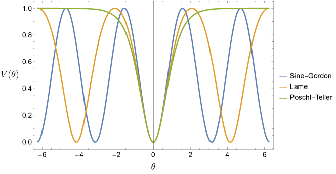
Starting with the limit approaching zero, one has and the Hamiltonian in this case
| (4.12) |
in which . This Hamiltonian is precisely the one of sine-Gordon quantum mechanics whose potential is periodic.
On the other hand, the one-dimensional model is also non-trivial in the other limit reaching the unity. Before proceeding to the reduced quantum mechanics, we briefly review some basic results of the deformed model in the large limit. From the two-dimensional perspective, the deformed model turns out to be the sausage/cigar model [59, 60] as the elongation becomes large [3]. And in the exact limit , or equivalently , the target space of the complex fields deforms to a cylinder [29] in the present limit. Namely,
| (4.13) |
On the one dimensional side, the Schrödinger equation (4.11) can be written as101010We have used the fact that .
| (4.14) |
in which now is defined on the half-real line . Certainly, the (4.14) is reflection invariant, and we can extend the domain from to . Note that Eq. (4.14) is recognized as the Pöschl-Teller system [61] and is also quasi-exactly solvable for judiciously chosen coefficient (cf. [10, 11].)
4.1 Comparison to Dunne-Shifman
As well-known in the literature, the Lamé model is Lie-algebraic and quasi-exactly solvable [11, 10, 57, 58, 12]. In other words, the associated Hamiltonian can be expressed as a matrix-valued function of a certain Lie algebra in some representation and a subset of the spectrum can be solved exactly. In [12], the Lamé system is studied in detail and shown that there exists a duality between bands and gaps in the spectrum. In the following, we detail the condition when our system is algebraic and its connection to the boundary condition imposed in the Scherk-Schwarz reduction. Without loss of generality, we may set and the circumference of the compactified dimension to be the unity for convenience.
To this end, recall that in the original construction of the Lie-algebraic sigma model [1, 2, 3], the differential representation of -algebra in the spin- representation is
| (4.15) |
where is a semi-integer and
| (4.16) |
following [12]. Then (4.11) is recast in the form
| (4.17) |
For (4.17) to be Lie-algebraic, there should be no dependence on the variable in the Hamiltonian. Hence, one requires that111111The dimension of can be recovered by taking .
| (4.18) |
Note that with the condition (4.18), the coefficient of the potential term in (4.11) is a multiple of satisfying the quasi-exactly solvable condition [12, 11]. As discussed in the dimensional reduction process, the constant depends on the boundary condition. Unlike (4.8) obtained under periodic boundary condition, the condition specified in Eq. (4.18) necessitates the imposition of the twisted boundary condition
| (4.19) |
4.2 Generalizations
So far, we have provided a comprehensive discussion on the relation between quasi-exactly solvable quantum mechanics and the Lamé quantum mechanics, as derived from dimensional reduction through a specific scheme. In Sec. 2, we also see some generalizations to the bosonic deformed model. Let us examine how these additional elements in the extended deformed model influence the corresponding quantum mechanics.
4.2.1 Reduction of the deformed model with twisted masses
In the case of the deformed model with twisted mass (2.28), one has
| (4.20) |
in which the fermionic part is ignored for the time being. Then, taking the same elliptic parametrization (4.3) and going through the same dimensnional reduction process, one deduces the Hamiltonian with twisted mass
| (4.21) |
By introducing an additional mass parameter, we can relax the twisted boundary condition as specified in Eq. (4.19), and instead, define a quantization condition for the mass parameter to satisfy the Lie-algebraic criterion. For example, let us keep the periodic boundary condition (4.8) intact. Then the quantization condition for the system to be QES is
| (4.22) |
for and . Similar treatments can be applied to anti-periodic and other boundary conditions along the compactified dimension.
4.2.2 Supersymmetric Lamé model
Another direction to generalize the Lamé model is to supersymmetrize it. Generally speaking, a supersymmetric quantum mechanics deformed by a potential term takes the form (see for example [14])
| (4.23) |
where is the superpotential and the matrix representation of fermions is adopted. By projecting onto the subspaces of different fermion numbers, the Hamiltonian (4.23) can be further simplified to an effective bosonic system, namely,
| (4.24) |
In particular, in the supersymmetric Lamé quantum mechanics, we have
| (4.25) |
with the Schrödinger equation . Note that the superpotential121212Here the parameter comparing to the previous case. in our case is
| (4.26) |
With the potential in Eq. (4.25) at hand, the supersymmetry is manifest, but this is not the case of Lie-algebraicity. The later part of this section is devoted to this issue.
Before moving on to the discussion on the Lie-algebraic structure of the supersymmetric Lamé QM, let us have a closer look at other interesting features of this system. First, we note that (4.25) is compatible with the 2D construction (2.1.2) and the dimensional reduction scheme. To see this is the case, in addition to (4.6), one also needs the reduction of the fermions
| (4.27) |
with the same boundary condition as the scalar fields. As a result, the reduced one-dimensional Lagrangian is
| (4.28) |
where is the normalized fermion field via velbein. This Lagrangian is obtained from (2.1.2) by substituting and within the compactification scheme (4.6) and (4.27) and integration over . It implies that the Hamiltonian indeed matches with the one proposed in (4.25) by taking and to be and , respectively, in the matrix representation. The ordering of the fermions is fixed such that the original Hamiltonian is where are supercharges.
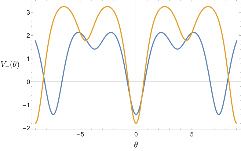
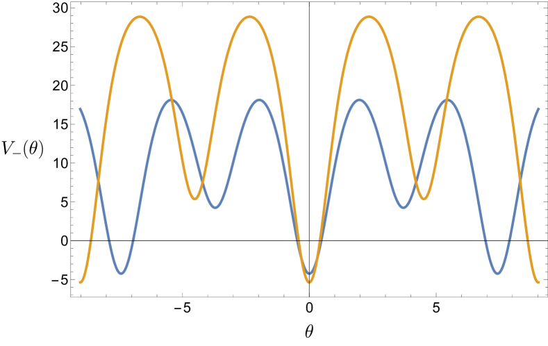
Lastly, the potential of the SUSY quantum mechanical model is depicted in figure 4. It is clear that the potential is periodic with period due to it elliptic function nature. As the value of increases, it is observed that the period is halved compared to cases with smaller . This is because the portion of the potential modified by the supersymmetric effect (or, equivalently, the presence of Weyl fermions) is proportional to , whereas the non-supersymmetric part of the potential is proportional to and has a period of . Furthermore, if one intend to conduct analysis via the WKB perturbation, it is noteworthy that there exist two distinct types of instanton events in the inverted potential: one involves tunneling through a tall barrier, while the other occurs via a low barrier.
Lie-algebraic features of supersymmetric Lamé Hamiltonian
To advance our understanding on the Lie-algebraic nature of the supersymmetric Lamé model, let us analyze the potential terms in the Hamiltonian in detail. In accordance with the argument in [58], the Hamiltonian (4.25), especially the last term, does not match the general form of the quasi-exactly solvable model with a double-periodic potential. However, this is not the end the story. The system can be transformed into a Lie-algebraic form via an appropriate coordinate transformation, though the quasi-exactly solvable condition requires separate verification. The aforementioned assertion is elaborated as follows. Consider the coordinate transformation
| (4.29) |
where
| (4.30) |
Utilizing the identities of Jacobi elliptic functions, we rephrase the corresponding Schrödinger equation of (4.25) in terms of dual variables
| (4.31) |
which fits into the Lie-algebraic form given in [58]. The Hamiltonian (4.31) is not the in the canonical form of SUSY QM. However, we can use the identity of the Jacobi elliptic functions presented in Appendix A such that the dual superpotential is
| (4.32) |
Then, the Lie-algebraic feature of the system is realized by the similar differential representation in (4.15), but with a different variable
| (4.33) |
Note that the Hamiltonian is formulated in the general form
| (4.34) |
with
| (4.35) |
The other coefficients and can be derived from the consistency condition (D.1) given in [58]. The derivation is tedious, but straightforward and we left further illustrations in Appendix D. The complete set of solutions to (D.1) can be categorized into three groups, as summarized in Table 1. Qualitative discussions on this set of solutions and some examples of specific representations are provided as follows.
To start with, note that the group (A1) in Table 1 with conincides with the supersymmetric ground state. To see this is the case, for , there are no contributions from and , but from the constant term, which is . On the other hand, we have from the right-handed side of (4.31) that
| (4.36) |
implying the vanishing of the ground state energy.
Generally speaking, due to the existence of the solutions in Table 1 to consistency equations, one would hence conclude that the supersymmetric is quasi-exactly solvable. In other words, the tasks of solving the differential equation for the eigenstates and eigenenergy are then translated to the problem of solving eigenvalues and eigenvectors of matrices of the spin- representations of algebra. The explicit matrix form of the dual Hamiltonian can be found by inserting the solutions given in table 1 to the general expression (4.34). However, this observation does not hold universally across all values of as some eigenvalues emerge as complex for these specific values. We consider some numerical investigations on the eigenvalues of the dual Hamiltonian for different sets of solutions in Table 1.
Here we give the examples of quasi-exact solvability of some lower spin representations, for instance, and . For the spin- sector, the Hamiltonian takes the forms
| (4.37a) | ||||
| (4.37b) | ||||
| (4.37c) | ||||
with eigenvalues
| (4.38a) | ||||
| (4.38b) | ||||
| (4.38c) | ||||
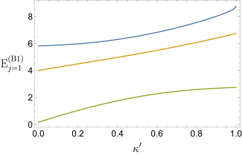
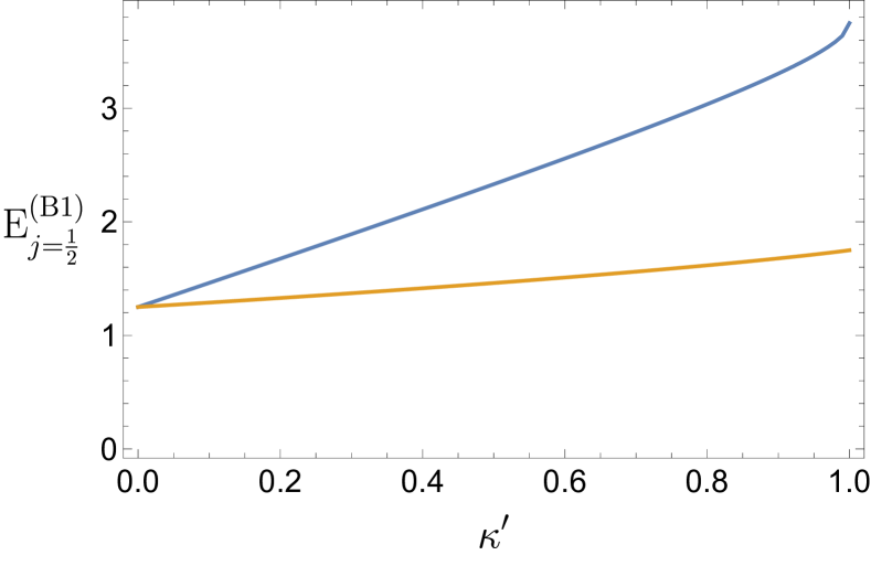
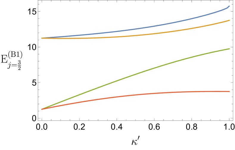
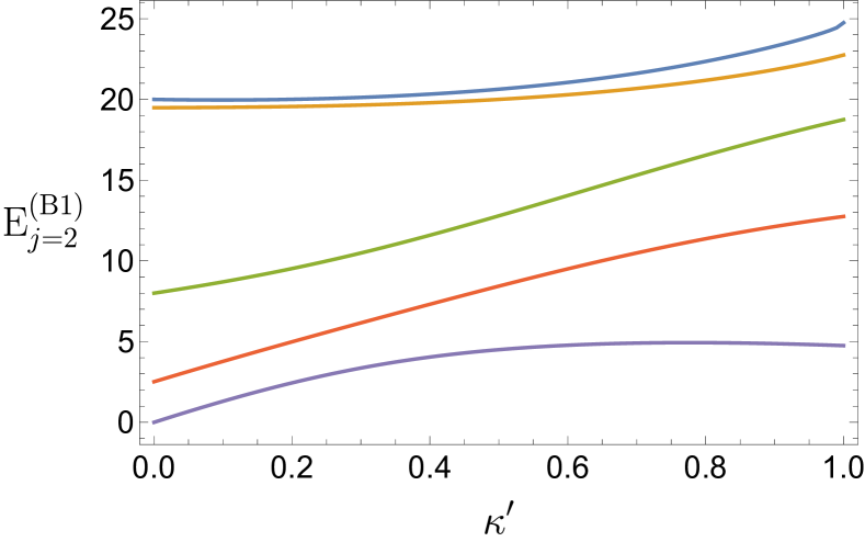
The energy of the group (A1) with is real for all . Regarding case (B1) and (B2), it is observed that the elements in the square roots of Eq. (4.38b) and (4.38c) remains non-negative for . This signifies that the system is fully quasi-exactly solvable across the entire interval for all three parametrization. In the spin-1 sector, a slightly different observation is made as in the spin- scenario, where the associated energy within the group (B2) is real over a specific interval of . Meanwhile, the energy for groups (A1) and (B1) remains real across the entire range of . This is most effectively illustrated by figure 5, given that the expressions for the dual Hamiltonians are lengthy and their physical meaning is not immediately clear from their precise formulations. The energy of the eigenstates of the dual Hamiltonian for are depicted in figure 6.
To wrap up the current section, we comment on the supersymmetric Lamé model with twisted masses. By employing the same steps as outlined earlier, one can similarly derive the supersymmetric Lamé model. The configuration of the potential terms remains nearly identical to that of the model without twisted masses, with the primary distinction being in the associated coefficients. Namely,
| (4.39) |
in which we assume is real for simplicity. Also, we can expect that this system is Lie-algebraic and quasi-exactly solvable because the twisted mass as an additional parameter increases the degree of freedom of (D.1).
5 Conclusions and outlooks
In our study, we explored various aspects related to the Lie-algebraic deformation of the sigma model in two dimensions. We stated from generalizing the original model endowing it with heterotic and extended supersymmetries. Then, we identified the hypercurrent anomaly in both scenarios. Notably, in the extended supersymmetry case, the anomaly, while being one-loop, deviates from conventional formulations found in the literature [20] due to the non-symmetric nature of the target Kähler manifold. We further elucidated the incorporation of twisted masses and the term and examined the BPS equation for instantons, focusing on its connection to the topological charge.
Moreover, we established that the second-loop contribution to the function in the non-supersymmetric Lie-algebraic sigma model arises from an infrared phenomenon. We used a supersymmetric regularization to substantiate our findings. We suggest that this inference extends to higher loops, drawing a parallel with similar behaviors observed in four-dimensional super-Yang-Mills theory.
In the second half of the paper, we point out the relationship between the Lie-algebraically deformed model and Lamé-type quantum mechanics, achieved through the Scherk-Schwarz dimensional reduction technique. This result is then further generalized to the case of supersymmetry. Upon certain additional requirements, the supersymmetric quantal problem obtained in this way proves to be quasi-exactly solvable. Further research into the link between two-dimensional Lie-algebraic models and quasi-exactly solvable quantum mechanics could focus on the deformation of 2D sigma models via specific potentials and the generalization of Lamé quantum mechanics, including the study of the associated Lamé equation.
Acknowledgments
M.S. is grateful to A. Turbiner and O. Gamayun for useful discussions. This work is supported in part by DOE grant DE-SC0011842 and the Simons Foundation Targeted Grant 920184 to the Fine Theoretical Physics Institute.
Appendices
Appendix A Conventions on elliptic integrals and Jacobi elliptic function
In this appendix, we provide a summary of the definitions and several useful identities of Jacobi elliptic functions that are used in the main text. Further properties can be found in, for example, [62, 63]. First, the elliptic integral of the first kind is defined as
| (A.1) |
where the complete elliptic integral . To define Jacobi elliptic functions, it suffices to consider the inverse of the incomplete integral
| (A.2) |
Then the Jacobi elliptic functions are represented as
| (A.3) |
with the elliptic modulus and .
The following identities are used in discussion of the Lamé systems, in particular, in Sec. 4 for the dual transformations,
| (A.4) |
Appendix B Derivation of anomalous axial currrent
In this section, we outline the derivation of the connection between the divergence of the anomalous axial current and the theta term of the deformed model.
Parallel to the discussion in [64], one has that
| (B.1) |
where is the regularization function with cutoff such that
Here we consider the vielbein to decompose the metric, say,
| (B.2) |
and the covariant derivative under this frame is
Consequently, the trace turns out to be
| (B.3) |
To get the second line of (B), we take the limit and employ the commutation relation
in which
| (B.4) |
Therefore, combining (B.1) and (B), we have
| (B.5) |
Appendix C Comparison between deformed quantum mechanics and Lamé quantum mechanics
Here the distinction between different dimensional reduction scenarios are detailed. In particular, we compare the resultant quantum mechanics from the Kaluza–Klein (KK) and the Scherk-Schwarz reductions.
In the Kaluza–Klein framework, one assumes the spacetime dependence of the field to be
| (C.1) |
As substituting this into (1.3), integrating along the -direction, and keeping only the lowest mode, we have
| (C.2) |
from which we can see that there will be some additional pieces in the deformed Hamiltonian, comparing with the Lamé equation. Indeed, according to Eq. (C.2), the Hamiltonian of the deformed model is
| (C.3) |
where is the Laplace operator. Note that (C.2) is a two-dimensional quantum mechanical system while the Lamé model (4.11) is of one dimension which depends only on . Thus even we consider the zero-angular momentum sector of the Hilbert space (i.e. ), there is still an additional linear contribution in in the deformed Hamiltonian than the Lamé one. If one keeps a higher mode rather than the lowest one, it will introduce an extra mass term, but can still do nothing with eliminating the linear differential part in . The further discussion on the deformed quantum mechanics derived from the KK reduction can be found in [65]. In fact, the similar issue between the model and the sine-Gordon model was discussed in [66] from the perspective of resurgence analysis.
Appendix D Details of Lie-algebraic features of supersymmetric Lamé quantum mechanics
The sufficient and necessary condition for rendering the system quasi-exactly solvable is that there exists non-trivial solutions to the equations of consistency131313These consistent equations arise from the change of variables from to . given in [58], namely,
| (D.1a) | ||||
| (D.1b) | ||||
| (D.1c) | ||||
| (D.1d) | ||||
For group (A1), it corresponds to taking while taking is related to group (B1) and (B2).
References
- [1] O. Gamayun, A. Losev, and M. Shifman, Peculiarities of beta functions in sigma models, JHEP 10 (2023) 097, arXiv:2307.04665 [hep-th].
- [2] O. Gamayun, A. Losev, and M. Shifman, First-order formalism for functions in bosonic sigma models from supersymmetry breaking, arXiv:2312.01885 [hep-th].
- [3] C.-H. Sheu and M. Shifman, Remarks on baby Skyrmion Lie-algebraic generalization, Phys. Rev. D 108 (2023) 065003, arXiv:2303.12597 [hep-th].
- [4] L. Alvarez-Gaume and D. Z. Freedman, Potentials for the Supersymmetric Nonlinear Sigma Model, Commun. Math. Phys. 91 (1983) 87.
- [5] M. Shifman, A. Vainshtein, and R. Zwicky, Central charge anomalies in 2-D sigma models with twisted mass, J. Phys. A 39 (2006) 13005–13024, arXiv:hep-th/0602004.
- [6] M. A. Shifman and A. I. Vainshtein, Solution of the Anomaly Puzzle in SUSY Gauge Theories and the Wilson Operator Expansion, Nucl. Phys. B 277 (1986) 456.
- [7] X. Cui and M. Shifman, N=(0,2) Deformation of CP(1) Model: Two-dimensional Analog of N=1 Yang-Mills Theory in Four Dimensions, Phys. Rev. D 85 (2012) 045004, arXiv:1111.6350 [hep-th].
- [8] J. Chen, X. Cui, M. Shifman, and A. Vainshtein, N=(0,2) deformation of (2, 2) sigma models: Geometric structure, holomorphic anomaly, and exact functions, Phys. Rev. D 90 (2014) 045014, arXiv:1404.4689 [hep-th].
- [9] N. Arkani-Hamed and H. Murayama, Holomorphy, rescaling anomalies and exact beta functions in supersymmetric gauge theories, JHEP 06 (2000) 030, arXiv:hep-th/9707133.
- [10] A. V. Turbiner, One-dimensional quasi-exactly solvable Schrödinger equations, Phys. Rept. 642 (2016) 1–71, arXiv:1603.02992 [quant-ph].
- [11] M. A. Shifman, New Findings in Quantum Mechanics (Partial Algebraization of the Spectral Problem), Int. J. Mod. Phys. A 4 (1989) 2897. [Extended version: in ITEP Lec- tures on Particle Physics and Field Theory, (World Scientific, 1999) Vol .2, 775-875; available at https://lib-extopc.kek.jp/preprints/PDF/1998/9807/9807055.pdf].
- [12] G. V. Dunne and M. Shifman, Duality and selfduality (energy reflection symmetry) of quasiexactly solvable periodic potentials, Annals Phys. 299 (2002) 143–173, arXiv:hep-th/0204224.
- [13] L. Alvarez-Gaume and D. Z. Freedman, Geometrical Structure and Ultraviolet Finiteness in the Supersymmetric Sigma Model, Commun. Math. Phys. 80 (1981) 443.
- [14] K. Hori, S. Katz, A. Klemm, R. Pandharipande, R. Thomas, C. Vafa, R. Vakil, and E. Zaslow, Mirror symmetry, Clay mathematics monographs I, AMS, Providence, USA, 2003. [http://www.claymath.org/library/monographs/cmim01.pdf].
- [15] A. M. Perelomov, Supersymmetric chiral models: Geometrical aspects, Phys. Rept. 174 (1989) 229–282.
- [16] E. Witten, Two-dimensional models with (0,2) supersymmetry: Perturbative aspects, Adv. Theor. Math. Phys. 11 (2007) 1–63, arXiv:hep-th/0504078.
- [17] M. Shifman and A. Yung, Heterotic Flux Tubes in N=2 SQCD with N=1 Preserving Deformations, Phys. Rev. D 77 (2008) 125016, arXiv:0803.0158 [hep-th]. [Erratum: Phys.Rev.D 79, 049901 (2009)].
- [18] X. Cui and M. Shifman, Perturbative Aspects of Heterotically Deformed CP(N-1) Sigma Model. I, Phys. Rev. D 82 (2010) 105022, arXiv:1009.4421 [hep-th].
- [19] M. A. Shifman and A. I. Vainshtein, Solution of the Anomaly Puzzle in SUSY Gauge Theories and the Wilson Operator Expansion, Nucl. Phys. B 277 (1986) 456.
- [20] Z. Komargodski and N. Seiberg, Comments on Supercurrent Multiplets, Supersymmetric Field Theories and Supergravity, JHEP 07 (2010) 017, arXiv:1002.2228 [hep-th].
- [21] T. T. Dumitrescu and N. Seiberg, Supercurrents and Brane Currents in Diverse Dimensions, JHEP 07 (2011) 095, arXiv:1106.0031 [hep-th].
- [22] A. Losev and M. Shifman, N=2 sigma model with twisted mass and superpotential: Central charges and solitons, Phys. Rev. D 68 (2003) 045006, arXiv:hep-th/0304003.
- [23] M. Shifman, Advanced Topics in Quantum Field Theory, Cambridge University Press, 2 ed., 2022.
- [24] S. J. Gates, Jr., Superspace Formulation of New Nonlinear Sigma Models, Nucl. Phys. B 238 (1984) 349–366.
- [25] S. J. Gates, Jr., C. M. Hull, and M. Rocek, Twisted Multiplets and New Supersymmetric Nonlinear Sigma Models, Nucl. Phys. B 248 (1984) 157–186.
- [26] N. Dorey, The BPS spectra of two-dimensional supersymmetric gauge theories with twisted mass terms, JHEP 11 (1998) 005, arXiv:hep-th/9806056.
- [27] L. Alvarez-Gaume, D. Z. Freedman, and S. Mukhi, The Background Field Method and the Ultraviolet Structure of the Supersymmetric Nonlinear Sigma Model, Annals Phys. 134 (1981) 85.
- [28] D. H. Friedan, Nonlinear Models in Dimensions, Annals Phys. 163 (1985) 318.
- [29] D. Bykov and A. Pribytok, Supersymmetric deformation of the model and its conformal limits, arXiv:2312.16396 [hep-th].
- [30] M. Alfimov, I. Kalinichenko, and A. Litvinov, On -function of supersymmetric integrable sigma-models, arXiv:2311.14187 [hep-th].
- [31] M. T. Grisaru, A. E. M. van de Ven, and D. Zanon, Four Loop beta Function for the N=1 and N=2 Supersymmetric Nonlinear Sigma Model in Two-Dimensions, Phys. Lett. B 173 (1986) 423–428.
- [32] L. Alvarez-Gaume and P. H. Ginsparg, Finiteness of Ricci Flat Supersymmetric Nonlinear Sigma Models, Commun. Math. Phys. 102 (1985) 311.
- [33] L. Alvarez-Gaume, S. R. Coleman, and P. H. Ginsparg, Finiteness of Ricci Flat Supersymmetric Models, Commun. Math. Phys. 103 (1986) 423.
- [34] N. Seiberg and E. Witten, Electric - magnetic duality, monopole condensation, and confinement in N=2 supersymmetric Yang-Mills theory, Nucl. Phys. B 426 (1994) 19–52, arXiv:hep-th/9407087. [Erratum: Nucl.Phys.B 430, 485–486 (1994)].
- [35] N. Seiberg and E. Witten, Monopoles, duality and chiral symmetry breaking in N=2 supersymmetric QCD, Nucl. Phys. B 431 (1994) 484–550, arXiv:hep-th/9408099.
- [36] K. Higashijima and M. Nitta, Kahler normal coordinate expansion in supersymmetric theories, Prog. Theor. Phys. 105 (2001) 243–260, arXiv:hep-th/0006027.
- [37] K. Higashijima, E. Itou, and M. Nitta, Normal coordinates in Kahler manifolds and the background field method, Prog. Theor. Phys. 108 (2002) 185–202, arXiv:hep-th/0203081.
- [38] S. V. Ketov, Quantum nonlinear sigma models, Springer-Verlag, 2000.
- [39] L. Alvarez-Gaume and D. Z. Freedman, Kähler Geometry and the Renormalization of Supersymmetric Sigma Models, Phys. Rev. D 22 (1980) 846.
- [40] N. A. Nekrasov, Seiberg-Witten prepotential from instanton counting, Adv. Theor. Math. Phys. 7 (2003) 831–864, arXiv:hep-th/0206161.
- [41] M. Shifman and A. Yung, NonAbelian string junctions as confined monopoles, Phys. Rev. D 70 (2004) 045004, arXiv:hep-th/0403149.
- [42] A. Hanany and D. Tong, Vortex strings and four-dimensional gauge dynamics, JHEP 04 (2004) 066, arXiv:hep-th/0403158.
- [43] M. A. Shifman and A. I. Vainshtein, On holomorphic dependence and infrared effects in supersymmetric gauge theories, Nucl. Phys. B 359 (1991) 571–580.
- [44] N. Arkani-Hamed and H. Murayama, Holomorphy, rescaling anomalies and exact beta functions in supersymmetric gauge theories, JHEP 06 (2000) 030, arXiv:hep-th/9707133.
- [45] V. A. Novikov, M. A. Shifman, A. I. Vainshtein, and V. I. Zakharov, Exact Gell-Mann-Low Function of Supersymmetric Yang-Mills Theories from Instanton Calculus, Nucl. Phys. B 229 (1983) 381–393.
- [46] K. V. Stepanyantz, Derivation of the exact NSVZ -function in N=1 SQED, regularized by higher derivatives, by direct summation of Feynman diagrams, Nucl. Phys. B 852 (2011) 71–107, arXiv:1102.3772 [hep-th].
- [47] K. V. Stepanyantz, The NSVZ -function for theories regularized by higher covariant derivatives: the all-loop sum of matter and ghost singularities, JHEP 01 (2020) 192, arXiv:1912.12589 [hep-th].
- [48] K. Stepanyantz, The all-loop perturbative derivation of the NSVZ -function and the NSVZ scheme in the non-Abelian case by summing singular contributions, Eur. Phys. J. C 80 (2020) 911, arXiv:2007.11935 [hep-th].
- [49] J. Chen, X. Cui, M. Shifman, and A. Vainshtein, On isometry anomalies in minimal = (0,1) and = (0,2) sigma models, Int. J. Mod. Phys. A 31 (2016) 1650147, arXiv:1510.04324 [hep-th].
- [50] J. Chen, X. Cui, M. Shifman, and A. Vainshtein, Anomalies of minimal and sigma models on homogeneous spaces, J. Phys. A 50 (2017) 025401, arXiv:1511.08276 [hep-th].
- [51] H. J. W. Müller-Kirsten, Introduction to Quantum Mechanics: Schrödinger Equation and Path Integral, World Scientific, 2012.
- [52] L. Brink, A. Turbiner, and N. Wyllard, Hidden algebras of the (super)Calogero and Sutherland models, J. Math. Phys. 39 (1998) 1285–1315, arXiv:hep-th/9705219.
- [53] A. Turbiner, Lie algebras and linear operators with invariant subspaces, arXiv:funct-an/9301001.
- [54] A. Turbiner, Quasiexactly solvable differential equations, arXiv:hep-th/9409068.
- [55] J. Scherk and J. H. Schwarz, How to Get Masses from Extra Dimensions, Nucl. Phys. B 153 (1979) 61–88.
- [56] T. Misumi, M. Nitta, and N. Sakai, Resurgence in sine-Gordon quantum mechanics: Exact agreement between multi-instantons and uniform WKB, JHEP 09 (2015) 157, arXiv:1507.00408 [hep-th].
- [57] A. V. Turbiner, Lame Equation, Sl(2) Algebra and Isospectral Deformations, J. Phys. A 22 (1989) L1.
- [58] A. Ganguly, Associated Lamé equation, periodic potentials and sl(2,R), Mod. Phys. Lett. A 15 (2000) 1923, arXiv:math-ph/0204026.
- [59] V. A. Fateev, E. Onofri, and A. B. Zamolodchikov, Integrable deformations of the sigma model. The sausage model, Nucl. Phys. B 406 (1993) 521–565.
- [60] S. L. Lukyanov and A. B. Zamolodchikov, Integrability in 2 fields theory/sigma models, Les Houches Lect. Notes 106 (2019) .
- [61] A. O. Barut, A. Inomata, and R. Wilson, Algebraic Treatment of Second Poschl-teller, Morse-rosen and Eckart Equations, J. Phys. A 20 (1987) 4083.
- [62] “NIST Digital Library of Mathematical Functions.”. https://dlmf.nist.gov/, release 1.1.12 of 2023-12-15.
- [63] M. Abramowitz and I. Stegun, Handbook of Mathematical Functions with Formulas, Graphs, and Mathematical Tables, Dover, New York, ninth dover printing, tenth gpo printing ed., 2013.
- [64] K. Fujikawa and H. Suzuki, Path integrals and quantum anomalies, Oxford University Press, 2004.
- [65] C.-H. Sheu, Perturbative and non-perturbative features in the lie-algebraic sigma model with chiral fermions, in preparation .
- [66] T. Fujimori, S. Kamata, T. Misumi, M. Nitta, and N. Sakai, Nonperturbative contributions from complexified solutions in models, Phys. Rev. D 94 (2016) 105002, arXiv:1607.04205 [hep-th].