Circuit Knitting Faces Exponential Sampling Overhead
Scaling Bounded by Entanglement Cost

Abstract

Circuit knitting, a method for connecting quantum circuits across multiple processors to simulate nonlocal quantum operations, is a promising approach for distributed quantum computing. While various techniques have been developed for circuit knitting, we uncover fundamental limitations to the scalability of this technology. We prove that the sampling overhead of circuit knitting is exponentially lower bounded by the exact entanglement cost of the target bipartite dynamic, even for asymptotic overhead in the parallel cut regime. Specifically, we prove that the regularized sampling overhead assisted with local operations and classical communication (LOCC), of any bipartite quantum channel is lower bounded by the exponential of its exact entanglement cost under separable preserving operations. Furthermore, we show that the regularized sampling overhead for simulating a general bipartite channel via LOCC is lower bounded by $\kappa$-entanglement and max-Rains information, providing efficiently computable benchmarks. Our work reveals a profound connection between virtual quantum information processing via quasi-probability decomposition and quantum Shannon theory, highlighting the critical role of entanglement in distributed quantum computing.

1 Introduction

Quantum computing stands poised to revolutionize information processing by leveraging the peculiar properties of quantum mechanics. Distributed quantum computing (DQC) [1], as one of the exciting frontiers in the Noisy intermediate-scale quantum (NISQ) [2] era, seeks to interconnect multiple quantum processors to form a unified and more powerful computing system. It provides a concept to overcome the physical connectivity challenge [3] and stands as the fundamental of quantum networks and quantum algorithms [4, 5].

Among numerous schemes, circuit knitting was proposed as a significant stride toward a near-term DQC [6, 7, 8] and simulating quantum many-body dynamics [9, 10, 11, 12]. It is believed of central importance to use the quasi-probability decomposition (QPD)  [13, 14, 15] for simulating the bipartite quantum channels. In particular, a linear combination of local operation and classical communication (LOCC) channels can make the target channel by individually executing them on separate parties. Subsequently, the results from sampling these operations can yield the same outputs as from directly constructing the intended target channel. Therefore, this modular approach promises to facilitate the construction of large-scale quantum circuits and has recently attracted attention in the research of quantum error mitigation [16, 17, 18, 19, 7, 20], simulation algorithms [21, 22, 11] and quantum resource theory [23, 24, 25].

Despite its potential, circuit knitting faces critical challenges threatening its scalability and practical implementation [7]. One such challenge comes from the sampling cost associated with the QPD technique, which could exhibit exponential growth with the increase in the size and complexity of the quantum circuit [7]. This rapid escalation in resource demands poses a significant barrier to the scalability of the circuit knitting method, potentially questioning its viability for large-scale DQC. Besides, the factors that dominate the sampling cost of realizing bipartite quantum channels stay ambiguous. Further optimization of the technique is, therefore, hindered by a lack of guidance.

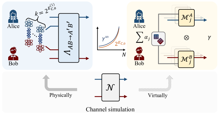
Fig 1: Illustration of the main result on the relevance between the exact (parallel) entanglement cost $E_{C,0}$ of physically implementing a bipartite quantum channel ${\cal N}$ (left) and the regularized sampling overhead $\gamma^{\infty}$ from virtually simulating ${\cal N}$ using the circuit knitting technique (right). The one-shot exact entanglement cost $E_{C,0}^{(1)}$ quantifies the minimum entanglement shared by Alice and Bob to realize a bipartite quantum channel exactly. The implementation relies on a bipartite channel $\Lambda_{AB\rightarrow A^{\prime}B^{\prime}}$ from LOCC, SEP or PPT channels. The $\gamma$-factor quantifies the minimum sampling overhead of simulating ${\cal N}$ using free operations. Our results demonstrate the fundamental limitation of the circuit knitting technique by establishing an exponential lower bound of $\gamma^{\infty}$ with respect to $E_{C,0}$ of ${\cal N}$ in order to simulate an asymptotic number of ${\cal N}$.

Entanglement is a fundamental resource in quantum computation and quantum information, playing crucial roles in quantum teleportation [26], fast quantum algorithms [27], and quantum error correction [28]. These various applications have motivated us to investigate the role of entanglement in the circuit knitting tasks. In quantum information theory, the exact (parallel) entanglement cost of a bipartite quantum channel was introduced to represent the minimum rates of maximally entangled states consumed for realizing simultaneous uses of it with zero-error [29, 30, 31]. Such a quantifier has been applied to studies on entanglement manipulation, channel resource theory, and information amortization [29, 30, 32]. Inspired by the research on entanglement, we then naturally question,

• What is the relationship between the sampling overhead of circuit knitting and the entanglement cost of a bipartite channel?

The concept of the entanglement cost can be traced back to [28] as an upper bound for quantum channel capacities. Later on, the entanglement cost of point-to-point quantum channels, i.e., the channel with one input and one output systems, has been investigated for decades and has developed gorgeous results, including the relationship towards entanglement of formation [33] and quantum channel simulation [34]. Recent literature has extended the ideas to the bipartite scenarios and delineated the definitions [29, 31]. In general, estimating the entanglement cost of a bipartite quantum channel is extremely hard due to the complex framework of superchannels, causal ordering, and regularization calculations [35, 29]. Recent works have derived the nontrivial and efficiently computable lower bounds of exact (parallel) cost of bipartite channels via the assistance of completely positive-partial-transposed preserving (PPT) operations [29, 30] where the PPT conditions inspire many information-theoretical discoveries in entanglement theory, quantum reversed Shannon theory and quantum resource theory [36, 30, 37, 38]. $E_{\kappa}$ (or $LN_{\max}$) is so-call the $\kappa$-entanglement which was introduced in [29, 30] to upper bound the exact entanglement cost of quantum channels.

In this work, we try to answer the question above by establishing the quantitative relationship between the two ways of channel simulations (Fig 1). We reveal the fundamental limitations of circuit knitting by establishing an exponential lower bound with respect to the number of qubits on the regularized sampling cost for a bipartite quantum channel. Technically, we connect the regularized sampling cost of a bipartite quantum channel with its entanglement cost. In particular, we show the following

$$\gamma_{{\text{\rm LOCC}}}^{\infty}({\cal N}_{AB\rightarrow A^{\prime}B^{\prime}})\geq 2^{E^{{\text{\rm SEP}}}_{C,0}({\cal N}_{AB\rightarrow A^{\prime}B^{\prime}})},\;\gamma_{{\text{\rm PPT}}}^{\infty}({\cal N}_{AB\rightarrow A^{\prime}B^{\prime}})\geq 2^{E^{{\text{\rm PPT}}}_{C,0}({\cal N}_{AB\rightarrow A^{\prime}B^{\prime}})}$$ (1)

where $\gamma_{{\text{\rm LOCC}}}^{\infty}({\cal N}),\gamma_{{\text{\rm PPT}}}^{\infty}({\cal N})$ are LOCC-assisted and PPT-assisted regularized sampling cost of ${\cal N}_{AB\rightarrow A^{\prime}B^{\prime}}$, respectively. $E^{{\text{\rm SEP}}}_{C,0}({\cal N}_{AB\rightarrow A^{\prime}B^{\prime}})$ and $E^{{\text{\rm PPT}}}_{C,0}({\cal N}_{AB\rightarrow A^{\prime}B^{\prime}})$ are the exact entanglement cost of ${\cal N}_{AB\rightarrow A^{\prime}B^{\prime}}$ via PPT bipartite operations and separable (SEP) bipartite operations, respectively [30, 29]. We further establish efficiently computable lower bounds for the regularized $\gamma$-factor utilizing the bidirectional max-Rains information [39] and $\kappa$-entanglement [29] of any bipartite channels, which can be efficiently estimated via semidefinite programming (SDP). Notably, our results apply to general bipartite channels instead of specific bipartite unitaries, and break through the barrier of KAK decomposition [40] mainly used in previous literature [13, 7].

The setting of circuit knitting in this work follows the assumptions in Ref. [7]. We consider a quantum circuit divided into two parties, namely $A$ and $B$, which contain $n$ bipartite channels across two parties, e.g., noisy bipartite quantum gates. Our results show that the total number of samples required for exactly simulating the entire circuit scales $\Omega(4^{\widehat{E}_{{\text{\rm SEP}},C}}\log(1/\epsilon)/\delta^{2})$ by QPD method, regarding the estimation error $\delta$ and failure probability $\epsilon$, where $\widehat{E}_{{\text{\rm SEP}},C}$ denotes the maximum one-shot exact entanglement cost assisted with separable channels, among these $n$ channels. We also raise case studies on noisy two- and three-qubit gates, such as CNOT, Toffoli, and control SWAP gates, and showcase the different costs via different partitioning.

Our studies give a deeper understanding of the scalability problem for circuit knitting, indicating that, even with shared bound entanglement [41, 42, 43], the sampling cost might still not be reduced from the exponential-growing catastrophe [7]. Despite the fundamental limitations of circuit knitting from this work in terms of quantum Shannon theory, our discussion laterally implies the potential quantum advantages of entangling channels, which might not be simply replaced by the sampling simulation techniques.

This paper is structured as follows. Sec. 2 provides notations and preliminaries used throughout the paper. Sec. 3 introduces two perspectives of bipartite quantum channel simulation, including the QPD method for estimating expectation values and the conventional method using LOCC and entanglement. Sec. 4 exhibits the main results from our investigation, including the exponential lower bounds of regularized $\gamma$-factor regarding the entanglement cost of bipartite channels and computable quantum information measures. In Sec. 5, the arguments on the fundamental limitation of circuit knitting will be given provided the PPT-assisted QPD and our lower bound results. The paper concludes with a summary and outlooks for future research in Sec. 6.

2 Preliminaries

Notations. Let ${\cal H}$ be a finite-dimensional Hilbert space. Consider two parties, Alice and Bob, with associated Hilbert spaces ${\cal H}_{A}$ and ${\cal H}_{B}$, respectively, where the dimensions of ${\cal H}_{A}$ and ${\cal H}_{B}$ are denoted as $d_{A}$ and $d_{B}$. We use ${\cal L}({\cal H}_{A})$ to represent the set of linear operators on system $A$, ${\cal P}({\cal H}_{A})$ to represent the set of Hermitian and positive semidefinite operators, and ${\cal D}({\cal H}_{A})$ to represent the set of all density operators. A linear operator $\rho_{A}\in{\cal D}({\cal H}_{A})$ gives a general representation of a quantum state with its trace equal to one. The maximally entangled state of dimension $d\otimes d$ is denoted as $\Phi_{AB}(d)=1/d\sum_{i,j=0}^{d-1}|ii\rangle\!\langle jj|$. The trace norm of $\rho$ is denoted as $\|\rho\|_{1}=\operatorname{Tr}(\sqrt{\rho^{\dagger}\rho})$. A bipartite quantum state $\rho_{AB}\in{\cal D}({\cal H}_{A}\otimes{\cal H}_{B})$ is a linear operator acting on the product of Hilbert space ${\cal H}_{A}\otimes{\cal H}_{B}$. The state $\rho_{AB}$ is called a positive partial transpose (PPT) state on the composite system ${\cal H}_{AB}$ if ${\cal T}_{B}(\rho_{AB})=\rho_{AB}^{T_{B}}\geq 0$ where ${\cal T}_{B}$ denotes the partial transpose operation regarding the system $B$. The set of separable (SEP) states on the composite system ${\cal H}_{AB}$ (i.e. the states written at convex combinations of tensor product states) is a subset of all PPT states.

Quantum channels. A quantum channel ${\cal N}_{A\rightarrow A^{\prime}}$ is a completely positive trace-preserving (CPTP) linear map that transforms linear operators from ${\cal L}({\cal H}_{A})$ to ${\cal L}({\cal H}_{A^{\prime}})$. The Choi-Jamiołkowski operator of ${\cal N}_{A\rightarrow A^{\prime}}$ is expressed as $J^{{\cal N}}_{AA^{\prime}}=d_{A}({\cal I}_{\bar{A}}\otimes{\cal N})(\Phi_{\bar{A}A}(d_{A}))$. We use $\tilde{J}^{{\cal N}}_{AA^{\prime}}$ to denote the corresponding Choi state of the channel. A bipartite channel ${\cal N}_{AB\rightarrow A^{\prime}B^{\prime}}$ maps any linear operator in system $AB$ to system $A^{\prime}B^{\prime}$, i.e., ${\cal N}_{AB\rightarrow A^{\prime}B^{\prime}}\mathrel{\mathop{\mathchar 58\relax}}{\cal L}({\cal H}_{AB})\rightarrow{\cal L}({\cal H}_{A^{\prime}B^{\prime}})$. In particular, a separable (SEP) bipartite channel is represented as [44],

$${\cal S}_{AB\rightarrow A^{\prime}B^{\prime}}=\sum_{j}{\cal E}_{A\rightarrow A^{\prime}}^{j}\otimes{\cal F}_{B\rightarrow B^{\prime}}^{j},$$ (2)

where $\{{\cal E}_{A\rightarrow A^{\prime}}^{j}\}$ and $\{{\cal F}_{B\rightarrow B^{\prime}}^{j}\}$ are sets of completely positive, trace-non-increasing maps (CPTN) such that ${\cal S}_{AB\rightarrow A^{\prime}B^{\prime}}$ is trace preserving. Every SEP channel completely preserves the separability of quantum states and can not generate entanglement. An important example of a separable channel is the LOCC channel, which consists of local operations and classical communication. Further, a bipartite PPT channel completely preserves the PPT property of states, which satisfies ${\cal N}^{\Gamma_{B}}\coloneqq{\cal T}_{B^{\prime}}\circ{\cal N}\circ{\cal T}_{B}$ is CPTP. This has been proven that the Choi matrix of ${\cal N}$ must satisfy $(J^{{\cal N}}_{ABA^{\prime}B^{\prime}})^{T_{BB^{\prime}}}\succeq 0$ as for the state case.

3 Simulation of bipartite quantum channels

The simulation of a bipartite quantum channel can be understood from two perspectives. The first one utilizes some entangled states between the two parties to physically realize the bipartite channel via entanglement non-generating operations. The second one virtually simulates the channel by sampling quantum operations and post-processing, which can be used to estimate the expectation value of any physical observable after the state passes through the channel.

3.1 Simulation via Monte-Carlo method

Let us begin our discussion on the channel simulation task by sampling and post-processing. Given any bipartite quantum channel ${\cal N}_{AB\rightarrow A^{\prime}B^{\prime}}$, we target to find a set of real coefficients $\{\alpha_{j}\}$ and a set of LOCC $\{{\cal M}_{j}\}$ between ${\cal L}({\cal H}_{AA^{\prime}})$ and ${\cal L}({\cal H}_{BB^{\prime}})$ such that ${\cal N}=\sum_{j}\alpha_{j}{\cal M}_{j}$. The set $\{(\alpha_{j},{\cal M}_{j})\}$ forms a quasiprobability decomposition (QPD) of the channel ${\cal N}$ [13, 14, 15]. Such a QPD protocol of ${\cal N}$ enables the simulation method of ${\cal N}$ via randomly sampling ${\cal M}_{j}$’s with their regarding probability $|\alpha_{j}|/\kappa$ where $\kappa=\sum_{j}\lvert\alpha_{j}\rvert$. That is, for any (normalized) observable $O$ and input quantum state $\rho$, the expectation value of $O$ with respect to ${\cal N}(\rho)$ can be extracted by the Monte Carlo method.

By Hoeffding’s inequality, we require at least ${\cal O}(\frac{\kappa^{2}}{\delta^{2}}\ln{\frac{2}{\epsilon}})$ samples of ${\cal M}_{j}$ to achieve the estimation error $\delta$ with a probability $1-\epsilon$. Therefore, the sampling overhead defined as $\kappa$ determines the number of samples demanded to simulate ${\cal N}$. Among all possible LOCC-assisted QPD of ${\cal N}$, we could quantify the sampling cost of simulating ${\cal N}$ by identifying the minimum sampling overhead, denoted as $\gamma_{{\text{\rm LOCC}}}({\cal N})$ which also quantifies the nonlocality of given bipartite quantum channel [7]. Notice that the $\gamma$-factor is closely related to the generalized robustness of the quantum channel regarding specific channel sets and has been recently discussed in Ref. [12].

The definition of QPD for circuit knitting concerning other operation sets has been discussed in [7, 8]. The technique also inspires the ‘twisted channel’ framework for general measurement in Ref. [45].

3.2 Bipartite channel simulation via LOCC and entanglement

Compared to the QPD sampling simulation , the entanglement cost of a point-to-point quantum channel is defined as the minimal asymptotic rate of the maximally entangled state required to simulate $n$-use of the channel assisted with LOCC [33]. The framework was then extended to the more complex bipartite scenarios based on the channel simulation tasks [29, 31, 30] embedded in the framework of quantum comb [35]. To distinguish with the point-to-point cases, the entanglement cost of bipartite channels is more complicated, containing both sequential and parallel schemes. The former allows the amortization of information to enhance the simulation, while the other naturally forms a particular case of the sequential setting by consuming independent resources. In Refs. [29, 30], both independent works have developed efficiently computable lower bounds of the costs via the relaxation towards PPT superchannels.

In particular, given a bipartite quantum channel ${\cal N}_{AB\rightarrow A^{\prime}B^{\prime}}$, one can define the entanglement cost of ${\cal N}$ via the task of channel simulations [33, 29, 34, 30]. Two types of schemes, including the parallel and the adaptive simulation scheme, are used to define the entanglement cost of bipartite channels. Under the parallel framework, the goal is to simulate ${\cal N}^{\otimes n}$ simultaneously using some higher-dimensional free channels consuming maximally entangled states. Let us consider a simulation protocol ${\cal P}_{A^{n}B^{n}\rightarrow A^{\prime n}B^{\prime n}}$ such that for any input state $\rho_{A^{n}B^{n}}$, we have,

$${\cal P}_{A^{n}B^{n}\rightarrow A^{\prime n}B^{\prime n}}(\rho_{A^{n}B^{n}})\coloneqq\Lambda_{A^{n}B^{n}\bar{A}\bar{B}\rightarrow A^{\prime n}B^{\prime n}}(\rho_{A^{n}B^{n}}\otimes\Phi_{\bar{A}\bar{B}}),$$ (3)

where $\Lambda$ here is a free channel, e.g., LOCC-, PPT- or SEP-preserving channels. For $\varepsilon\geq 0$, we say the protocol is $\varepsilon$-distinguishable from ${\cal N}^{\otimes n}$ if,

$$\|{\cal N}_{AB\rightarrow A^{\prime}B^{\prime}}^{\otimes n}-{\cal P}_{A^{n}B^{n}\rightarrow A^{\prime n}B^{\prime n}}\|_{\diamond}\leq\varepsilon,$$ (4)

where $\|\cdot\|_{\diamond}$ is the diamond norm between linear maps [46]. Based on the channel simulation protocol, we can first define the one-shot entanglement cost of a bipartite channel,

Definition 1

Consider a bipartite system with parties Alice and Bob. Let $\varepsilon\geq 0$ and ${\cal N}_{AB\rightarrow A^{\prime}B^{\prime}}$ be a bipartite channel. The one-shot entanglement cost of ${\cal N}$ with error $\varepsilon$, regarding the free operation set ${\cal F}$, is defined as

$$E_{{\cal F},C,\varepsilon}^{(1)}({\cal N})\mathrel{\mathop{\mathchar 58\relax}}=\min\left\{\log k\,\mathrel{\mathop{\mathchar 58\relax}}\,\left\|{\cal N}_{AB\rightarrow A^{\prime}B^{\prime}}-\Lambda_{AB\bar{A}\bar{B}\rightarrow A^{\prime}B^{\prime}}(\ \cdot\otimes\Phi_{\bar{A}\bar{B}}^{\otimes k})\right\|_{\diamond}\leq\varepsilon,\,k\in\mathbb{N}\right\},$$ (5)

where the minimization ranges over all $\Lambda$ operations in ${\cal F}$ between Alice and Bob.

Therefore, the (parallel) ${\cal F}$-entanglement cost of bipartite channels can be defined as the asymptotic infimum rate of the entanglement resources to realize the protocol with zero error, i.e.,

$$E^{{\cal F}}_{C}({\cal N})\coloneqq\lim_{\varepsilon\rightarrow 0}\limsup_{n\rightarrow\infty}\frac{1}{n}E_{{\cal F},C,\varepsilon}^{(1)}({\cal N}^{\otimes n}).$$ (6)

We can also define the exact (parallel) ${\cal F}$-entanglement cost of ${\cal N}$ as,

$$E^{{\cal F}}_{C,0}({\cal N})\coloneqq\limsup_{n\rightarrow\infty}\frac{1}{n}E_{{\cal F},C,\varepsilon=0}^{(1)}({\cal N}^{\otimes n}),$$ (7)

which forms an upper bound of the asymptotic entanglement cost. In particular, if ${\cal F}={\text{\rm LOCC}}$, we could omit to label ‘${\cal F}$’ in the symbol of entanglement cost. Refer to the simulation of channels, in the single-shot scenario, one requires $\Phi_{\bar{A}\bar{B}}=\Phi_{\bar{A}_{0}\bar{B}_{1}}\otimes\Phi_{\bar{A}_{1}\bar{B}_{0}}$ and the free operation to simulate the SWAP operation ${\cal S}$ where $\bar{A}=\bar{A}_{0}\otimes\bar{A}_{1}$ and $\bar{B}=\bar{B}_{0}\otimes\bar{B}_{1}$. In the parallel setting, one can, therefore, treat the SWAP operation as the maximal resource for dynamical entanglement [29, 31]. Notice that, taking the dimension $|B|=|A^{\prime}|=1$, the above definition is naturally reduced to the entanglement cost of the point-to-point channel. Another definition of the entanglement cost of bipartite channels, namely the sequential or adaptive cost, has been also generally discussed in Refs. [29, 30], forming a lower bound of the parallel entanglement cost.

4 Sampling cost is exponentially lower bounded by entanglement cost

Despite many efforts that have been made recently, the computation of the $\gamma$-factor for knitting arbitrary bipartite quantum channels via LOCC stays challenging. Besides, the relationship between the sampling cost and the entanglement theory of bipartite channels has not been completely built. In this section, we first introduce the settings of circuit knitting and the definitions of the exact regularized $\gamma$-factor from the point of resource theory. In subsection 4.1, we introduce the PPT-assisted $\gamma$-factor and derive the exponential lower bound of its regularized form with respect to the NPT exact entanglement cost, and provide an efficiently computable upper bound of it via SDP. In subsection 4.2, we further tighten the two sides of the theorem towards the LOCC scenario by proving the similar relationship for separable channels.

With the optimal QPD of ${\cal N}$, we can imagine a situation of a quantum circuit containing $n$ identical bipartite channels ${\cal N}$ applied to the two parties of the quantum circuit which is used in some quantum computing task. For example, in the estimation of the ground state energy of the Hamiltonian via variational ansatz [47] and simulation of quantum many-body dynamics [12]. One can avoid generating global entanglement by individually decomposing those entangling operations across the two subcircuits. Unfortunately, this would result in an exponential growth in sampling overhead [7].

From the perspective of quantum resource theory, Ref. [7] has introduced parallel cutting for circuit knitting to reduce sampling cost-effectively. Consider a circuit with $n$ multiple gates $(U_{j})_{j=1}^{n}$, which we wish to cut them simultaneously instead of cutting each individual of them. In that case, the entire cut can be observed as a single cut on the total circuit $U_{tot}=\bigotimes_{j=1}^{n}U_{j}$ via some pre-processes using local swap operations. We can define the effective sampling overhead per gate of cutting [7] as,

$$\gamma^{(n)}_{{\cal F}}({\cal N}_{AB\rightarrow A^{\prime}B^{\prime}})\coloneqq(\gamma_{{\cal F}_{n}}({\cal N}_{AB\rightarrow A^{\prime}B^{\prime}}^{\otimes n}))^{1/n},$$ (8)

where ${\cal F}_{n}$ is the free operation set of $n$-shot. The optimal strategy from joint cut indicates the limitation of cutting $U_{tot}$ into QPD and the total number of samples required can gain significant reduction from $\prod_{j=1}^{n}\gamma_{{\cal F}}({\cal U}_{j})^{2}$ to $\prod_{j=1}^{n}\gamma^{(n)}_{{\cal F}}({\cal U}_{j})^{2}$. Despite the subtleties that determining $U_{tot}$ itself is as challenging as implementing the entire circuit directly [8], we can still define the regularized exact $\gamma$-factor with respect to the free operation set ${\cal F}$ by taking the limit $n\rightarrow\infty$ for any bipartite channel ${\cal N}$, i.e., $\gamma_{{\cal F}}^{\infty}({\cal N})\coloneqq\lim_{n\rightarrow\infty}\gamma_{{\cal F}}^{(n)}({\cal N})$, which quantifies the fundamental limitation on the sampling cost from simulating ${\cal N}$ using circuit knitting.

4.1 PPT-assisted sampling cost and NPT exact entanglement cost

The $\gamma$-factor was proven to be closely related to the robustness of entanglement [7, 48]. The quantity has been thoroughly studied in [49] for resource distillation tasks. To further demonstrate the advantages of circuit knitting techniques, it is crucial to investigate the connection between the sampling cost and the actual resource cost of veritably implementing the bipartite channels.

In the NPT entanglement theory, PPT channels are commonly applied in studies on the properties and limitations of LOCCs. Based on Refs. [29, 30, 31], one can define the exact PPT-entanglement cost of any bipartite channel ${\cal N}_{AB\rightarrow A^{\prime}B^{\prime}}$ by letting ${\cal F}={\text{\rm PPT}}$ in Eq. (7) and it is known that $E^{{\text{\rm PPT}}}_{C,0}({\cal N}_{AB\rightarrow A^{\prime}B^{\prime}})$ is smaller than or equal to the max-logarithmic negativity or generalized $\kappa$-entanglement $LN_{\max}\left({\cal N}_{AB\rightarrow A^{\prime}B^{\prime}}\right)$, i.e., $E^{{\text{\rm PPT}}}_{C,0}({\cal N}_{AB\rightarrow A^{\prime}B^{\prime}})\leq LN_{\max}\left({\cal N}_{AB\rightarrow A^{\prime}B^{\prime}}\right)$, and

$$LN_{\max}\left({\cal N}_{AB\rightarrow A^{\prime}B^{\prime}}\right)=\log \inf\Big{\{}\max\left\{\left\|P_{AB}\right\|_{\infty},\left\|P_{AB}^{T_{B}}\right\|_{\infty}\right\}\mathrel{\mathop{\mathchar 58\relax}}$$ (9)

$$-P_{ABA^{\prime}B^{\prime}}^{T_{BB^{\prime}}}\leq\left(J_{ABA^{\prime}B^{\prime}}^{{\cal N}}\right)^{T_{BB^{\prime}}}\leq P_{ABA^{\prime}B^{\prime}}^{T_{BB^{\prime}}},\,P_{ABA^{\prime}B^{\prime}}\geq 0\Big{\}}.$$

The max-logarithmic negativity of a bipartite channel can be computed via SDP [30], which is a generalization of $\kappa$-entanglement [50] for the bipartite channels. It is called max-logarithmic negativity since it can be understood as the maximum case of the $\alpha$-logarithmic negativity [51].

Based on the above, our first result is to establish the relationship between $\gamma_{{\text{\rm PPT}}}({\cal N}_{AB\rightarrow A^{\prime}B^{\prime}})$ and the exact PPT-entanglement cost of the channel.

The detailed proof is in Appendix B. We remark that the last inequality is not an equality as presented in [31] due to the non-additivity of max-logarithmic negativity or $\kappa$-entanglement [52, 53].

On the other hand, we have also derived another efficiently computable lower bound of $\gamma^{\infty}_{{\text{\rm PPT}}}({\cal N})$ via the technique of max-Rains information [54], whose bidirectional version was applied to establish the upper bound for entanglement generating capacity of any bipartite channels [39]. Our second computable lower bound of $\gamma_{{\text{\rm PPT}}}$ is given as follows,

$$\gamma^{\infty}_{{\text{\rm PPT}}}({\cal N})\geq 2^{R_{\max}^{2\rightarrow 2}({\cal N})}.$$ (11)

The max-Rains information of a bipartite quantum channel ${\cal N}_{AB\rightarrow A^{\prime}B^{\prime}}$ is defined as,

$$R_{\max}^{2\rightarrow 2}({\cal N})\coloneqq\log(\Gamma^{2\rightarrow 2}({\cal N})),$$ (12)

where $\Gamma^{2\rightarrow 2}({\cal N})$ can be evaluated via the SDP,

$$\Gamma^{2\rightarrow 2}({\cal N})=\inf\{\|\operatorname{Tr}_{AB}\{V_{AA^{\prime}BB^{\prime}}+Y_{AA^{\prime}BB^{\prime}}\}\|_{\infty}\mathrel{\mathop{\mathchar 58\relax}}V,Y\geq 0,(V-Y)^{T_{BB^{\prime}}}\geq J^{{\cal N}}_{AA^{\prime}BB^{\prime}}\}.$$ (13)

One can compare both efficiently computable lower bounds for PPT-assisted $\gamma$-factor and illustrate them in Fig. 2. Since our bounds work for general bipartite channels, we can then apply our bounds to investigate the variations of sampling cost for noisy gates. For example, consider the noisy CNOT gate ${\cal N}_{p}={\cal D}_{p}\circ{\cal C}{\cal X}$ where ${\cal D}_{p}$ is the general two-qubit depolarizing (DE) channel. For any two-qubit state $\rho_{AB}$, we have,

$${\cal N}_{p}(\rho_{AB})\coloneqq(1-p)\operatorname{CNOT}\rho_{AB}\operatorname{CNOT}+p\frac{I_{AB}}{d_{AB}}.$$ (14)

As we can observe from the figure, when there is no noise occurring, $\gamma_{{\text{\rm PPT}}}({\cal N}_{p})$ can reach $3$ from our SDP calculation. This is the same value as from the LOCC results of the CNOT gate in Ref. [7], indicating no advantages of using bipartite PPT channels in QPD. The two lower bounds from $LN_{\max}$ and $R_{\max}^{2\rightarrow 2}$ both start at $2$, indicating at least one ebit is required to implement a CNOT with PPT or LOCC. When $p\geq 0.9$, too much noise destroys the entangling power of the CNOT gate, and all values are reduced to one.

From Fig. 2, we observe that the two lower bounds coincide with each other. This does not hold for general cases. We provide the following counterexample to show the relative size of the two bounds. Suppose now a SWAP gate is applied where the second qubit is accidentally stroked by the qubit amplitude damping (AD) channel ${\cal A}_{\gamma}$ defined by its Kraus operators

$$K_{0}=|0\rangle\!\langle 0|+\sqrt{1-\gamma}|1\rangle\!\langle 1|,\,K_{1}=\sqrt{\gamma}|0\rangle\!\langle 1|.$$ (15)

AD channel models the loss of quantum information when a quantum system interacts with its thermal bath. Our noisy SWAP operation is then defined as

$${\cal S}_{\gamma}(\rho_{AB})\coloneqq({\cal I}_{A}\otimes{\cal A}_{\gamma})\left(\operatorname{SWAP}\rho_{AB}\operatorname{SWAP}\right)$$ (16)

for any two-qubit state $\rho_{AB}\in{\cal D}({\cal H}_{AB})$. The results have been shown in Fig. 3 where a distinct gap between the one-shot $\gamma_{{\text{\rm PPT}}}({\cal S}_{\gamma})$ and the two lower bounds can be identified. Notice that $LN_{\max}({\cal S}_{\gamma})$ does not necessarily equal to $R_{\max}^{2\rightarrow 2}({\cal S}_{\gamma})$, where in this case, the max logarithmic negativity bound is slightly larger than the max-Rains information bound as the damping rate varies.

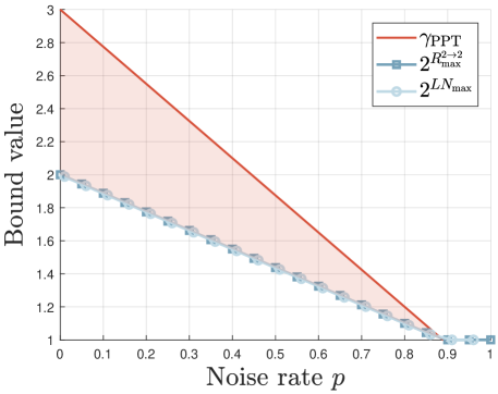
Fig 2: Lower bounds comparison for noisy CNOT operation undertaking the two-qubit depolarizing channel by the noise rate $p$. The orange solid line gives the one-shot exact $\gamma_{{\text{\rm PPT}}}({\cal N})$. The dark and light blue dashed lines with square and circle markers illustrate the lower bounds of regularized PPT $\gamma$-factor by max-Rains information and the max logarithmic negativity, respectively. The shaded area is the possible region for $\gamma_{{\text{\rm PPT}}}^{\infty}({\cal N})$ to lie in.

4.2 SEP-assisted sampling cost and SEP exact entanglement cost

In the previous section, we have extended the set of LOCC operations to PPT operations for more theoretical convenience. Here, we concentrate on a smaller free operation set ${\cal F}={\text{\rm SEP}}$, namely the separable-preserving channels defined in [30]. A bipartite channel is separable if and only if its Choi matrix is separable. Therefore, every separable quantum channel, at the same time, forms a PPT channel which implies that $\gamma_{{\text{\rm PPT}}}({\cal N})\leq\gamma_{{\text{\rm SEP}}}({\cal N})$. Besides, each above entanglement cost measure regarding SEP channels forms an upper bound of the corresponding PPT-entanglement cost. The set of SEP channels also serves as a candidate for investigating the properties of LOCC channels in quantum information theory, despite, detecting the separability of any quantum states is NP-hard [55].

Inspired by the entanglement manipulation for quantum states [56], we can establish a tighter bound towards LOCC-assisted circuit knitting. As before, the investigations of single-shot exact $\gamma$-factor and the SEP-entanglement cost of ${\cal N}$ further induce the relationship between the regularizations of both quantities, and we can establish the following theorem for the SEP-assisted circuit knitting.

The detailed proof can be found in Appendix C. Through the computable bound from PPT operations, one may allow ‘too much’ freedom to make a coarse relaxation for LOCC entanglement. Our ultimate goal is to establish the LOCC sampling cost lower bound by the exponential LOCC entanglement cost of given bipartite channels. All separable operations form a much more restricted set compared to PPT operations, and contains all LOCC channels. Despite their unrealizability in some cases, to our best knowledge, the usage of SEP channels leads to much tighter bounds for both the sampling cost and the entanglement costs compared to the PPT results, i.e., $\gamma^{\infty}_{{\text{\rm SEP}}}({\cal N})\leq\gamma^{\infty}_{{\text{\rm LOCC}}}({\cal N})$ and $E^{{\text{\rm SEP}}}_{C}({\cal N})\leq E_{C}({\cal N})$. As a consequence, combining all of the above results, one can derive the following remark connecting both the LOCC circuit knitting sampling complexities and the entanglement cost measures of bipartite quantum channels,

Remark 1

For any bipartite quantum channel ${\cal N}_{AB\rightarrow A^{\prime}B^{\prime}}$, the following inequalities holds,

$$\gamma^{\infty}_{{\text{\rm PPT}}}({\cal N})\geq 2^{E_{C,0}^{{\text{\rm PPT}}}({\cal N})}\geq 2^{E_{C}^{{\text{\rm PPT}}}({\cal N})},$$ (18)

$$\gamma^{\infty}_{{\text{\rm SEP}}}({\cal N})\geq 2^{E_{C,0}^{{\text{\rm SEP}}}({\cal N})}\geq 2^{E_{C}^{{\text{\rm SEP}}}({\cal N})}.$$

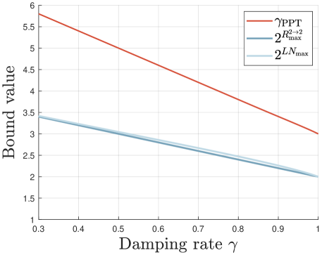
Fig 3: Lower bounds comparison for noisy SWAP operation undertaking the single-qubit amplitude damping channel by the damping rate $\gamma$. The orange solid line gives the one-shot exact $\gamma_{{\text{\rm PPT}}}({\cal N})$. The dark and light blue lines illustrate the lower bounds by max-Rains information and the max logarithmic negativity, respectively.

We can also demonstrate that the LOCC regularized $\gamma$-factor is exponentially lower bounded by the entanglement cost of ${\cal N}$ if ${\cal N}$ forms a bicovariant channel [29], for example, CNOT. The proof of this can be found in Appendix E. However, whether or not the above relation holds in general stays open, and we leave this for future investigation.

5 Fundamental limitation of circuit knitting

In previous sections, we have demonstrated the quantitative relation between the sampling cost of simulating a general bipartite channel via circuit knitting and the corresponding entanglement cost of the channel. Our theorem proves the intuition that the more entanglement resource cost for physically implementing the channel, the harder it is to simulate it via sampling LOCC channels combined with post-measurement selections. Based on the results, we attempt to establish the fundamental limitation of the circuit knitting technique in this section: in subsection 5.1, we revisit the sampling cost for some important quantum logic gates via new bounds; in subsection 5.2, we investigate the exponential growth of sampling cost for simulating multiple instances of bipartite channels in a more practical scenario.

5.1 Sampling cost for specific gates

The investigation of both the CNOT and SWAP gates stands at the central position of both quantum circuit architecture [57] and quantum information theory. A CNOT gate and a Bell state are commonly treated as equivalent resources of entanglement since a CNOT gate can be constructed via gate teleportation consuming one Bell state [58]. A SWAP gate owns the maximal resource of dynamical entanglement [31], which can generate two ebits shared with bi-parties. Besides, CNOT itself, together with single-qubit Pauli gates, forms a universal set for realizing any logic gates [59], while the SWAP gate is closely related to the general two-qubit Clifford gates [7].

As a start, we apply our theories to some specific gates, including CNOT and SWAP, and derive the same results as from previous research [7]. Since ${\text{\rm LOCC}}\subsetneq{\text{\rm SEP}}\subsetneq{\text{\rm PPT}}$, for single-shot exact $\gamma$-factor, we already have,

$$\gamma_{{\text{\rm LOCC}}}({\cal N})\geq\gamma_{{\text{\rm SEP}}}({\cal N})\geq\gamma_{{\text{\rm PPT}}}({\cal N})$$ (19)

for any general bipartite channel ${\cal N}$. Despite that, our result indicates that for a class of bipartite channels, the assistance of PPT-entanglement might contribute an insignificant advantage in reducing the sample complexity from the circuit knitting method.

We particularly remark that for any two-qubit Clifford gates, there is no advantage in using the PPT-assisted QPD, and the $\gamma$-factors of the following bipartite gates are given by,

$$\gamma_{{\cal F}}(\rm CNOT) =3;$$ (20)

$$\gamma_{{\cal F}}(i\rm{SWAP})=\gamma_{{\cal F}}(\rm SWAP) =7,$$

where ${\cal F}\in\{{\text{\rm LOCC}},{\text{\rm SEP}},{\text{\rm PPT}}\}$. Regarding the origin of circuit knitting, understanding the properties of two-qubit Clifford gates holds significant importance in terms of quantum advantages. Notably, it has been established that every such gate can be constructed via the gates $\mathbb{I}$, $\rm{CNOT}$, $\rm{SWAP}$, and $i\rm{SWAP}$ up to local unitary gates. These lead to the unchanged PPT-assisted sampling overhead compared to the LOCC results from [7], and therefore, disproves the improvement from PPT-entanglement in circuit knitting on two-qubit Clifford gates.

To investigate the limitation of PPT-assisted knitting, we also involve the discussion on the parallel-cut scheme in this case, which has achieved benefits for cutting copies of a Clifford gate $U$ under LOCC [7]. Consider cutting $n$-copies of CNOT gates, one can derive,

$$\gamma_{{\cal F}}(\operatorname{CNOT}^{\otimes n})=2^{n+1}-1$$ (21)

for the same set of operations ${\cal F}$ stated before. With the additional quantum memory for storing entanglement, one can demonstrate that the exact effective sampling cost of PPT-assisted knitting for the CNOT gate reaches the same asymptotic value, i.e., $\gamma^{\infty}_{{\cal F}}(\operatorname{CNOT})=\lim_{n\rightarrow\infty}\gamma^{(n)}_{{\cal F}}(\operatorname{CNOT})=2$. The proof of the above remarks can refer to Appendix D. The corresponding CNOT evolution is called the bicovariant bidirectional channel [39]. The max-Rains information bound in Eq. (11) reduces to the standard Rains relative entropy [60, 61] of its Choi state, indicating no benefits from the assistance of PPT operations under parallel cutting of CNOT.

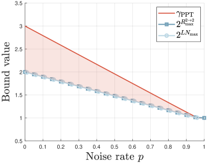
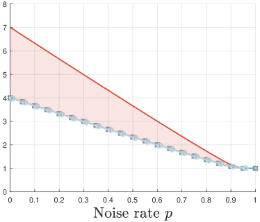
Fig 4: Lower bounds comparison for noisy control-SWAP operation (CSWAP) undertaking the global depolarizing channel by the noise rate $p$ with respect to different partitioning. The Left and right figures illustrate the bound values of cutting qubit $1$ and $2$ and qubit $2$ and $3$, respectively. The orange line gives the one-shot exact $\gamma_{{\text{\rm PPT}}}({\cal N})$. The dark and light blue lines with square and circle markers illustrate the lower bounds of regularized PPT $\gamma$-factor by max-Rains information and the max logarithmic negativity, respectively. The shaded area indicates that our bounds serve as feasible efficient-computable lower bounds for $\gamma_{{\text{\rm PPT}}}^{\infty}({\cal N})$.

Furthermore, our bound works for general bipartite quantum channels with non-equal dimensionalities of $A$ and $B$, instead of only unitary channels studied with [8] the KAK-decomposition [14]. It then serves as a useful tool for studying the nonlocality of non-KAK-like bipartite interactions and characterizing the optimal sampling overhead for non-unitary channels. For instance, the Toffoli gate is another important three-qubit gate discussed frequently in the quantum circuit architecture. Our observation showcases that,

$$\gamma^{(1)}_{{\cal F}}(\rm Toffoli)=\gamma^{(2)}_{{\cal F}}(\rm Toffoli)=3,$$ (22)

by setting a cut between the qubit 1-and-2 (1) or qubit 2-and-3 (2), as shown in [8], which acts as a tighter lower bound from the Choi state of the Toffoli gate. Interestingly, we have also tested the control-SWAP (CSWAP) gate, which is widely applied to quantum information tasks. In Fig. 4, compared to the results from Toffoli gate, the two cutting cases give very different values for the PPT-assisted $\gamma$-factor and the two lower bounds. Cutting between 1 and 2 qubits gives only half of the $\gamma$-factor from cutting 2 and 3 qubits. We observe that for general unitary cutting, the sampling cost may significantly vary by choosing different partitions.

5.2 Exponential cost for knitting multiple instances of bipartite channels

For a general bipartite quantum channel ${\cal N}_{AB\rightarrow A^{\prime}B^{\prime}}$, by the definition of parallel cutting, one can derive a lower bound for the $n$-effective sampling cost with finite $n$.

In the task of simulating $n\geq 1$ parallel instances of ${\cal N}$, we obtain that the optimal number of samples of circuit knitting with respect to the LOCC channels scales at least $\Omega(4^{nQ^{2\rightarrow 2}_{{\text{\rm LOCC}}}({\cal N})})$ delivering that the exponential growth in the sampling cost originates from the entanglement cost of its physical implementation. The number $n$ relates to the depth of the circuit, or the evolution time of the system, indicating the circuit knitting technique is generally inefficient for deep architectures. Besides, suppose the depth of the circuit is restricted. Only if $E^{{\text{\rm PPT}}}_{C,0}({\cal N})$ scales ${\cal O}(\log(N))$ where $N$ is the number of qubits in the system, the sampling cost can be polynomially lower bounded in $N$. In the large dimensional limit, only when ${\cal N}$ requires negligible entanglement resource to be implemented the lower bound of sampling cost from circuit knitting can gain reasonable scaling for practical usage.

We then extend our discussion to the quantum circuit containing $n\geq 1$ distinct bipartite quantum channels or the noisy quantum gates, as a reasonable assumption on NISQ devices, denoted as ${\cal N}_{1},\cdots,{\cal N}_{n}$. In the first scenario, each of these ${\cal N}_{j}$’s is aligned to parallel via local swaps as local operations can preserve the $\gamma$-factor of each ${\cal N}_{j}$. Given the aligned circuit as ${\cal N}=\bigotimes_{j=1}^{n}{\cal N}_{j}$, we directly derive the lower bound of $\gamma_{{\cal F}}({\cal N})$,

$$\gamma_{{\cal F}}\left({\cal N}\right)\geq\left(\prod_{j=1}^{n}2^{Q^{2\rightarrow 2}_{{\text{\rm LOCC}}}({\cal N}_{j})}\right)-1,$$ (24)

where we observe that if every ${\cal N}_{j}$ has insignificant entangling power, the product may tend to a constant scaling, and we may achieve an acceptable lower bound on $\gamma_{{\cal F}}({\cal N})$ for the practical implementation.

However, cutting the total circuit directly via the above is typically intractable as it requires tomography of ${\cal N}$. Otherwise, it may require smart channel grouping strategies to keep each term in the product of Eq. (24) sufficiently small. Instead, for each of these $n$ channels, suppose the corresponding ${\cal F}$-assisted QPD has been pre-determined and denote the associated optimal sampling overheads by $\gamma_{{\cal F}}({\cal N}_{j})$ for the $j$-th channel. Then, during each shot of execution on the circuit, we can only adopt the single cut strategy that ${\cal N}_{j}$ gets independently and randomly replaced by one of its QPD channels, which leads to a total number of samples required by at least $\gamma^{2}_{\rm tot}=\prod_{j=1}^{n}\gamma_{{\cal F}}({\cal N}_{j})^{2}$. We then derive the following corollary,

Suppose not all channels have zero entanglement cost, and we denote the maximum one-shot exact ${\cal F}$-entanglement cost among ${\cal N}_{j}$’s as $\widehat{E}_{{\cal F},C}$. Then, in the large dimension limit, the total sampling times via QPD can scale at least $\Omega(4^{\widehat{E}_{{\cal F},C}})$ by the dominant entangling channel.

If we assume the two parties of the system are isomorphic of dimension $d_{A}=d_{B}=d$, particularly for a qubit system, $d=2^{N}$ where $N$ is the number of qubits in the half circuit. Notice that for those channels with a small entanglement cost, there may exist classical simulation tools, for example, tensor network method [62], which can efficiently simulate the dynamics of the system going beyond $50$ qubits, and hence lose the meaning of accessing real quantum devices. Only those with sufficient entangling power can truly showcase the potential quantum advantages and worth to be applied with circuit knitting.

In fact, the entanglement cost of any bipartite channels can grow linearly in $N$ [63, 64]. which then leads to the scaling of $\gamma_{\rm tot}^{2}$ as $\Omega(4^{N})$ as also claimed in [7, 8]. Even with parallel cutting, we can derive that the total sampling cost based on the regularized form can scale at the same speed. Such an exponential growth in the sampling cost can not be avoided via the above strategies, which leads to the fundamental limitation of realizing the circuit knitting method on NISQ devices. From another perspective, the entangling channels are the quantum operations that can veritably showcase quantum advantages in computational tasks. Both the deterministic and the probabilistic simulation methods stated above via LOCC can be non-scalable and difficult.

6 Concluding remarks

In this work, we have unravelled the fundamental challenge of the circuit knitting technique by establishing the exponential lower bounds for the sampling cost and confirming that the more entanglement of the bipartite action, the more knitting cost is needed. In particular, we have proven the exponential correspondence of the regularized $\gamma$-factor with respect to the PPT- and SEP-entanglement cost of the nonlocal circuit that can be hardly avoided in the large dimension limit as long as the overall circuit across two parties carries non-negligible entangling capability. Our demonstration shows a $\Omega(4^{N})$ scaling of the sampling cost regarding the number of qubits $N$ in the half circuit from the perspective of quantum information theory, which coincides with previous literature [7].

Even allow more powerful operations such as PPT and SEP channels in QPD, our findings suggest that simulating any bidirectional interactions using the circuit knitting technique still experiences exponential growth in sampling cost compared to the LOCC-assisted scenario. For example, we prove the $\gamma$-factors from LOCC-, PPT- and SEP-QPD are identical for two-qubit Clifford gates. The results also serve as an extension from previous literature using KAK decomposition, which applies to general bipartite channels even with non-isomorphic biparties. We try to address the question raised in [8] by providing tighter lower bounds than the Schmidt decomposition bound from channel’s Choi state. Our numerical calculations also showcase distinct one-shot exact sample costs for the CSWAP gate with different partitioning.

Understanding the fundamental limitation of exponential sampling cost from circuit knitting regarding the entanglement cost of realizing any bipartite channel is crucial for future advancements in the field of distributed quantum computing. A few points would be interesting for further investigation, as stated. Apart from the parallel cutting for multiple instances of bipartite gates, we notice that the situation of composited channels has not yet been fully analyzed due to the trade-off between the cost of characterizing the entire process and the sampling cost of knitting the process. For example, the composition of two sequential CNOTs acting on the same pair of qubits may result in an identity. Such a ‘cancelling’ effect through the composition of gates provides a new insight for reducing the sampling cost of circuit knitting. Therefore, developing smart gate grouping and circuit compiling methods may provide a possible improvement in the circuit knitting technique. Besides, characterizing the minimum set of decomposition operations providing advantages in the sampling cost would be an important next step toward a deeper understanding of nonlocality and quantum entanglement. Such a set of operations may bring new life to the circuit knitting technique.

Appendix for: Circuit Knitting Faces Exponential Sampling Overhead
Scaling Bounded by Entanglement Cost

In these Supplementary Notes, we offer detailed proofs of the theorems and propositions in the manuscript ‘Fundamental limitation of circuit knitting for bipartite quantum channels’. In Appendix A, we first provide details of semidefinite programming (SDP) for PPT-assisted circuit knitting in terms of the $\gamma$-factor. Based on the formulation, we then prove the remark for specific two-qubit gates. In Appendix B & C, we prove our main theorems showing the exponential dependences between the regularized $\gamma$-factor and the exact entanglement cost of any given bipartite channels. In Appendix D, we also give another efficiently computable lower bound of the regularized PPT-assisted $\gamma$-factor using the bidirectional max-Rains information of the bipartite channels. In Appendix E, we introduce the concept of smoothed regularized LOCC-assisted $\gamma$-factor of any bipartite channel and showcase that it is, in fact, lower bounded via the vanishing error entanglement cost of its Choi state in the asymptotic regime. In Appendix F, we will give the analysis of the knitting cost for multiple distinct instances of bipartite quantum channels, including the proof of Corollary 3.

Throughout the paper, we label different quantum systems by capital Latin letters, e.g., $A,B$. The respective Hilbert spaces for these quantum systems are denoted as ${\cal H}_{A}$, ${\cal H}_{B}$, each with dimension $d_{A},d_{B}$. The set of all linear operators on ${\cal H}_{A}$ is denoted by ${\cal L}({\cal H}_{A})$, with $I_{A}$ representing the identity operator. We denote by ${\cal L}^{{\dagger}}({\cal H}_{A})$ the set of all Hermitian operators on ${\cal H}_{A}$. In particular, we denote ${\cal D}({\cal H}_{A})\subseteq{\cal L}^{{\dagger}}({\cal H}_{A})$ the set of all density operators being positive semidefinite and trace-one acting on ${\cal H}_{A}$. A linear map transforming linear operators in system $A$ to those in system $B$ is termed a quantum channel if it is completely positive and trace-preserving (CPTP), denoted as ${\cal N}_{A\rightarrow B}\mathrel{\mathop{\mathchar 58\relax}}{\cal L}({\cal H}_{A})\rightarrow{\cal L}({\cal H}_{B})$. The set of all quantum channels from $A$ to $B$ is denoted as $\text{\rm CPTP}(A,B)$.

The parallel cutting setting in this work is first introduced in Ref. [7] as shown in Fig. S1. Imagine the situation of cutting the circuit containing $n$ instances of bipartite noisy bipartite gates ${\cal N}_{1},{\cal N}_{2},\cdots,{\cal N}_{n}$. The optimal strategy of circuit knitting is to cut all the gates at the same time. To do so, one may have to first rearrange all the gates via local swap operations so that they become in parallel, i.e., ${\cal N}=\bigotimes_{j=1}^{n}{\cal N}_{j}$. The local swap operations can preserve the $\gamma$-factors as shown in [7].

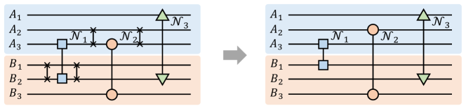
Fig S1: The strategy of aligning three bipartite noisy quantum gates to parallel via local SWAPs. ${\cal N}_{1},{\cal N}_{2}$ and ${\cal N}_{3}$ are originally acted on the qubit pairs $(A_{3},B_{2}),(A_{3},B_{3})$ and $(A_{1},B_{2})$, respectively.

Appendix A SDP formulation and remarks from PPT-assisted circuit knitting

The definition of PPT-assisted circuit knitting resembles the original definition of LOCC-assisted circuit knitting. Given any bipartite quantum channel ${\cal N}_{AB\rightarrow A^{\prime}B^{\prime}}$, one has to find a PPT-assisted quasi-probability decomposition (QPD) of it, i.e., ${\cal N}=c_{1}{\cal M}_{1}-c_{2}{\cal M}_{2}$ for some PPT channels ${\cal M}_{1,2}$ and positive coefficients $c_{1,2}$. Then the $\gamma$-factor $\gamma_{{\text{\rm PPT}}}({\cal N})$ can be estimated via the following semidefinite programming,

$$\gamma_{{\text{\rm PPT}}}({\cal N})=\min_{c_{1,2}\geq 0,\ J_{{\cal M}_{1,2}}} c_{1}+c_{2},$$ (S1)

$${\rm s.t.} J^{{\cal M}_{1,2}}_{ABA^{\prime}B^{\prime}}\succeq 0;\ (J^{{\cal M}_{1,2}}_{ABA^{\prime}B^{\prime}})^{T_{BB^{\prime}}}\succeq 0$$

$$J^{{\cal M}_{1}}_{AB}=c_{1}I_{AB};\ J^{{\cal M}_{2}}_{AB}=c_{2}I_{AB};$$

$$J^{{\cal N}}_{ABA^{\prime}B^{\prime}}=J^{{\cal M}_{1}}_{ABA^{\prime}B^{\prime}}-J^{{\cal M}_{2}}_{ABA^{\prime}B^{\prime}}.$$

For any arbitrary bipartite quantum channel ${\cal N}$, i.e., the completely positive trace-preserving (CPTP) maps, the last constraint in (S1) guarantee $c_{1}=c_{2}+1$ since for any state $\rho\in{\cal D}({\cal H}_{AB})$, we have

$$\operatorname{Tr}[{\cal N}(\rho)]=c_{1}\operatorname{Tr}[{\cal M}_{1}(\rho)]-c_{2}\operatorname{Tr}[{\cal M}_{2}(\rho)].$$

Therefore, we could rewrite the above SDP formulation for $\gamma_{{\text{\rm PPT}}}({\cal N})$ by eliminating $c_{2}$ and also the $J^{{\cal M}_{2}}_{ABA^{\prime}B^{\prime}}$. Writing $c=c_{1}$ and $J^{{\cal M}}_{ABA^{\prime}B^{\prime}}=J^{{\cal M}_{1}}_{ABA^{\prime}B^{\prime}}$, the objective function becomes $2c-1$. The constraint $J^{{\cal M}_{2}}_{ABA^{\prime}B^{\prime}}\succeq 0$ then becomes $J^{{\cal M}}_{ABA^{\prime}B^{\prime}}\succeq J^{{\cal N}}_{ABA^{\prime}B^{\prime}}$ and ${\cal T}_{BB^{\prime}}(J^{{\cal M}_{2}}_{ABA^{\prime}B^{\prime}})\succeq 0$ becomes ${\cal T}_{BB^{\prime}}(J^{{\cal M}}_{ABA^{\prime}B^{\prime}})\succeq{\cal T}_{BB^{\prime}}(J^{{\cal N}}_{ABA^{\prime}B^{\prime}})$. Notice that the second trace-preserving constraint then becomes automatically satisfied, and we derive the equivalent SDP for $\gamma_{{\text{\rm PPT}}}({\cal N})$,

$$\gamma_{{\text{\rm PPT}}}({\cal N})=\min_{c\geq 0,\ J_{{\cal M}}} 2c-1,$$ (S2)

$${\rm s.t.} (J^{{\cal M}}_{ABA^{\prime}B^{\prime}})^{T_{BB^{\prime}}}\succeq 0$$

$$J^{{\cal M}}_{AB}=cI_{AB};$$

$$J^{{\cal M}}_{ABA^{\prime}B^{\prime}}\succeq J^{{\cal N}}_{ABA^{\prime}B^{\prime}};$$

$$(J^{{\cal M}}_{ABA^{\prime}B^{\prime}})^{T_{BB^{\prime}}}\succeq(J^{{\cal N}}_{ABA^{\prime}B^{\prime}})^{T_{BB^{\prime}}},$$

Notice that the optimal value of $c$ from the above optimization is called the robustness of dynamical resource [65, 49], we have $\gamma_{{\text{\rm PPT}}}({\cal N})=2R_{{\text{\rm PPT}}}({\cal N})-1$. The value of $R_{{\text{\rm PPT}}}({\cal N})$ is closely related to the generalized robustness of PPT-entanglement [48, 49]. Notice that PPT operations are stronger than LOCC operations, this leads to $\gamma_{{\text{\rm LOCC}}}({\cal N})\geq\gamma_{{\text{\rm PPT}}}({\cal N})$. Therefore, for those two-qubit gates in the Remark, one direction has been proven referring to [7], which gives an equivalence argument for LO- and LOCC-assisted $\gamma$-factor. It suffices to prove the following,

$$\gamma_{{\text{\rm PPT}}}(\rm CNOT) \geq 3;$$ (S3)

$$\gamma_{{\text{\rm PPT}}}(i\rm{SWAP}) \geq 7;$$

$$\gamma_{{\text{\rm PPT}}}(\rm SWAP) \geq 7.$$

We prove these by first defining a new quantity $\widehat{W}({\cal N})$ which is derived from taking a relaxation on the programming of $R_{{\text{\rm PPT}}}({\cal N})$ by removing the constraint ${\cal T}_{BB^{\prime}}(J^{{\cal M}}_{ABA^{\prime}B^{\prime}})\succeq{\cal T}_{BB^{\prime}}(J^{{\cal N}}_{ABA^{\prime}B^{\prime}})$. The optimal value, which we denoted as $\widehat{W}({\cal N})$, can be estimated via the following SDP programming,

$$\widehat{W}({\cal N})=\min_{c\geq 0,\ J_{{\cal M}}} c,$$ (S4)

$${\rm s.t.} (J^{{\cal M}}_{ABA^{\prime}B^{\prime}})^{T_{BB^{\prime}}}\succeq 0;$$

$$J^{{\cal M}}_{ABA^{\prime}B^{\prime}}\succeq J^{{\cal N}}_{ABA^{\prime}B^{\prime}};$$

$$J^{{\cal M}}_{AB}\preceq cI_{AB}.$$

Clearly, we have, $R_{{\text{\rm PPT}}}({\cal N})\geq\widehat{W}({\cal N})$, therefore, $\gamma_{{\text{\rm PPT}}}({\cal N})\geq 2\widehat{W}({\cal N})-1$. We further derive the dual programming of (S4) follows by writing out the Lagrangian of the primal programming of $\widehat{W}({\cal N})$ as,

$$L(P,Q,R) =c-\operatorname{Tr}[P(J^{{\cal M}}_{ABA^{\prime}B^{\prime}})^{T_{BB^{\prime}}}]-\operatorname{Tr}[Q(J^{{\cal M}}_{ABA^{\prime}B^{\prime}}-J^{{\cal N}}_{ABA^{\prime}B^{\prime}})]$$ (S5)

$$\quad+\operatorname{Tr}[R(J^{{\cal M}}_{AB}-cI_{AB})],$$

$$=\operatorname{Tr}[QJ^{{\cal N}}_{ABA^{\prime}B^{\prime}}]+c(1-\operatorname{Tr}[R])+\operatorname{Tr}[J^{{\cal M}}_{ABA^{\prime}B^{\prime}}(R\otimes I_{A^{\prime}B^{\prime}}-P^{T_{BB^{\prime}}}-Q)]$$

where $P,Q,R\succeq 0$ are the introduced Lagrangian multipliers and $P,Q\in{\cal L}^{{\dagger}}({\cal H}_{ABA^{\prime}B^{\prime}})$, $R\in{\cal L}^{{\dagger}}({\cal H}_{AB})$. To ensure the dual function non-trivially lower bounded, we have $Q\preceq R\otimes I_{A^{\prime}B^{\prime}}-P^{T_{BB^{\prime}}}$ and $\operatorname{Tr}[R]\leq 1$. Taking the change of variables $Y=R\otimes I_{A^{\prime}B^{\prime}}-P^{T_{BB^{\prime}}}$ and due to Slater’s condition, the strong duality holds, and we have the following,

$$\widehat{W}({\cal N})=\max_{Y,Q\succeq 0,R} \operatorname{Tr}(QJ^{{\cal N}}_{ABA^{\prime}B^{\prime}})$$ (S6)

$${\rm s.t.} Q\preceq Y;\ Q,R\succeq 0;\operatorname{Tr}[R]\leq 1;$$

$$Y^{T_{BB^{\prime}}}\preceq R^{T_{B}}\otimes I_{A^{\prime}B^{\prime}}.$$

Notice that $Q$ can be now seen as a slackened variable by requiring $Y=Q$, and we, therefore, have the equivalent SDP,

$$\widehat{W}({\cal N})=\max_{Y,R\succeq 0} \operatorname{Tr}(Y_{ABA^{\prime}B^{\prime}}J^{{\cal N}}_{ABA^{\prime}B^{\prime}})$$ (S7)

$${\rm s.t.} \operatorname{Tr}[R_{AB}]\leq 1;$$

$$Y_{ABA^{\prime}B^{\prime}}^{T_{BB^{\prime}}}\preceq R_{AB}^{T_{B}}\otimes I_{A^{\prime}B^{\prime}}.$$

Now we are ready to prove the inequalities in (S3). Start with the CNOT operation. Notice that we could take $Y=J^{{\cal N}}_{ABA^{\prime}B^{\prime}}/8$ and $R_{AB}=I_{AB}/d_{AB}$ as a feasible solution to (S7) since $\operatorname{Tr}[R]=1$ and $|\operatorname{eig}[Y_{ABA^{\prime}B^{\prime}}^{T_{BB^{\prime}}}]|=|\operatorname{eig}[(J^{{\cal N}}_{ABA^{\prime}B^{\prime}})^{T_{BB^{\prime}}}]|/8\leq 1/4$. Therefore, the last constraint from (S7) holds and we have,

$$\widehat{W}({\cal N})\geq\frac{1}{8}\operatorname{Tr}[(J^{{\cal N}}_{ABA^{\prime}B^{\prime}})^{2}]=\frac{16}{8}=2,$$ (S8)

where $\operatorname{Tr}[(J^{{\cal N}}_{ABA^{\prime}B^{\prime}})^{2}]=4\operatorname{Tr}[J^{{\cal N}}_{ABA^{\prime}B^{\prime}}]=16$ as $J^{{\cal N}}_{ABA^{\prime}B^{\prime}}$ is unnormalized pure state for CNOT. We then have proven the statement for CNOT as $\gamma_{{\text{\rm PPT}}}(\rm{CNOT})\geq 4-1=3$. Similarly, we could take $Y=J^{{\cal N}}_{ABA^{\prime}B^{\prime}}/4,R_{AB}=I_{AB}$ as feasible solutions to $\rm{SWAP}$ and $i\rm{SWAP}$ as $|\operatorname{eig}[Y_{ABA^{\prime}B^{\prime}}^{T_{BB^{\prime}}}]|=|\operatorname{eig}[(J^{{\cal N}}_{ABA^{\prime}B^{\prime}})^{T_{BB^{\prime}}}]|/4\leq 1$, and therefore finish proofs for the remark.

Appendix B Proof of Theorem for regularized PPT-assisted sampling cost

In order to prove the exponential lower bound for the regularized PPT-assisted $\gamma$-factor with respect to the exact PPT-entanglement cost, we first prove the following lemma for the one-shot scenario.

Lemma S1

For a bipartite quantum channel ${\cal N}_{AB\rightarrow A^{\prime}B^{\prime}}$,

$$\gamma_{{\text{\rm PPT}}}({\cal N}_{AB\rightarrow A^{\prime}B^{\prime}})\geq 2^{LN_{\max}\left({\cal N}_{AB\rightarrow A^{\prime}B^{\prime}}\right)}-1.$$ (S9)

Proof.

Recalling the definition of $\gamma_{{\text{\rm PPT}}}({\cal N}_{AB\rightarrow A^{\prime}B^{\prime}})$ which can be re-expressed as

$$\gamma_{{\text{\rm PPT}}}({\cal N}_{AB\rightarrow A^{\prime}B^{\prime}})=\min \;2c-1$$ (S10)

$${\rm s.t.} \;J_{ABA^{\prime}B^{\prime}}^{{\cal N}}=cJ_{ABA^{\prime}B^{\prime}}^{{\cal M}_{1}}-(c-1)J_{ABA^{\prime}B^{\prime}}^{{\cal M}_{2}},$$

$$\;J_{ABA^{\prime}B^{\prime}}^{{\cal M}_{1}}\geq 0,\,J_{ABA^{\prime}B^{\prime}}^{{\cal M}_{2}}\geq 0,$$

$$\;(J_{ABA^{\prime}B^{\prime}}^{{\cal M}_{1}})^{T_{BB^{\prime}}}\geq 0,\,(J_{ABA^{\prime}B^{\prime}}^{{\cal M}_{2}})^{T_{BB^{\prime}}}\geq 0,$$

$$\;J_{AB}^{{\cal M}_{1}}=I_{AB},\,J_{AB}^{{\cal M}_{2}}=I_{AB}.$$

Suppose $\{J_{ABA^{\prime}B^{\prime}}^{{\cal M}_{1}},J_{ABA^{\prime}B^{\prime}}^{{\cal M}_{2}},c\}$ is a feasible solution for $\gamma_{{\text{\rm PPT}}}({\cal N})$. Then we have

$$(J_{ABA^{\prime}B^{\prime}}^{{\cal N}})^{T_{BB^{\prime}}}+(c-1)(J_{ABA^{\prime}B^{\prime}}^{{\cal M}_{2}})^{T_{BB^{\prime}}}\geq 0,\;c(J_{ABA^{\prime}B^{\prime}}^{{\cal M}_{1}})^{T_{BB^{\prime}}}-(J_{ABA^{\prime}B^{\prime}}^{{\cal N}})^{T_{BB^{\prime}}}\geq 0$$ (S11)

which yields

$$-(c-1)(J_{ABA^{\prime}B^{\prime}}^{{\cal M}_{2}})^{T_{BB^{\prime}}}\leq(J_{ABA^{\prime}B^{\prime}}^{{\cal N}})^{T_{BB^{\prime}}}\leq c(J_{ABA^{\prime}B^{\prime}}^{{\cal M}_{1}})^{T_{BB^{\prime}}}.$$ (S12)

By the fact that $(J_{ABA^{\prime}B^{\prime}}^{{\cal M}_{1}})^{T_{BB^{\prime}}}\geq 0$ and $(J_{ABA^{\prime}B^{\prime}}^{{\cal M}_{2}})^{T_{BB^{\prime}}}\geq 0$, we have

$$-(c-1)(J_{ABA^{\prime}B^{\prime}}^{{\cal M}_{1}}+J_{ABA^{\prime}B^{\prime}}^{{\cal M}_{2}})^{T_{BB^{\prime}}}\leq(J_{ABA^{\prime}B^{\prime}}^{{\cal N}})^{T_{BB^{\prime}}}\leq c(J_{ABA^{\prime}B^{\prime}}^{{\cal M}_{1}}+J_{ABA^{\prime}B^{\prime}}^{{\cal M}_{2}})^{T_{BB^{\prime}}}$$ (S13)

which further gives

$$-c(J_{ABA^{\prime}B^{\prime}}^{{\cal M}_{1}}+J_{ABA^{\prime}B^{\prime}}^{{\cal M}_{2}})^{T_{BB^{\prime}}}\leq(J_{ABA^{\prime}B^{\prime}}^{{\cal N}})^{T_{BB^{\prime}}}\leq c(J_{ABA^{\prime}B^{\prime}}^{{\cal M}_{1}}+J_{ABA^{\prime}B^{\prime}}^{{\cal M}_{2}})^{T_{BB^{\prime}}}.$$ (S14)

Let $P_{ABA^{\prime}B^{\prime}}=c(J_{ABA^{\prime}B^{\prime}}^{{\cal M}_{1}}+J_{ABA^{\prime}B^{\prime}}^{{\cal M}_{2}})$. We have that $P_{ABA^{\prime}B^{\prime}}$ is a feasible solution for $LN_{\max}\left({\cal N}_{AB\rightarrow A^{\prime}B^{\prime}}\right)$ and notice that by taking the partial trace on the subsystem $A^{\prime}B^{\prime}$, we have,

$$P_{AB}=P_{AB}^{T_{B}}=c(J_{AB}^{{\cal M}_{1}}+J_{AB}^{{\cal M}_{1}})=2c\cdot I_{AB}.$$ (S15)

Now we know that for each feasible solution $\{J_{ABA^{\prime}B^{\prime}}^{{\cal M}_{1}},J_{ABA^{\prime}B^{\prime}}^{{\cal M}_{2}},c\}$ of $\gamma_{{\text{\rm PPT}}}({\cal N}_{AB\rightarrow A^{\prime}B^{\prime}})$ with an objective value $2c-1$, there exists a feasible solution for $LN_{\max}({\cal N}_{AB\rightarrow A^{\prime}B^{\prime}})$ that gives an objective value less or equal to $\log(2c)$. Therefore, we have,

$$2^{LN_{\max}({\cal N}_{AB\rightarrow A^{\prime}B^{\prime}})}\leq 2c$$ (S16)

$$\Rightarrow \ \gamma_{{\text{\rm PPT}}}({\cal N}_{AB\rightarrow A^{\prime}B^{\prime}})\geq 2^{LN_{\max}({\cal N}_{AB\rightarrow A^{\prime}B^{\prime}})}-1.$$

By the fact that $E^{{\text{\rm PPT}}}_{C,0}({\cal N}_{AB\rightarrow A^{\prime}B^{\prime}})\leq LN_{\max}({\cal N}_{AB\rightarrow A^{\prime}B^{\prime}})$, we can also conclude that

$$\gamma_{{\text{\rm PPT}}}({\cal N}_{AB\rightarrow A^{\prime}B^{\prime}})\geq 2^{E^{{\text{\rm PPT}}}_{C,0}({\cal N}_{AB\rightarrow A^{\prime}B^{\prime}})}-1.$$ (S17)

$\sqcap$$\sqcup$

Remark 2

Since the exact entanglement cost of NPT-entanglement is no smaller than the exact distillable NPT-entanglement, which is no smaller than NPT entanglement generating power [31, 39, 66], i.e.,

$$E^{{\text{\rm PPT}}}_{D}({\cal N}_{AB\rightarrow A^{\prime}B^{\prime}})\leq E_{C}^{{\text{\rm PPT}}}({\cal N}_{AB\rightarrow A^{\prime}B^{\prime}})$$ (S18)

we can obtain similar lower bounds for $\gamma_{{\text{\rm PPT}}}({\cal N}_{AB\rightarrow A^{\prime}B^{\prime}})$ correspondingly up to a constant factor.

Proof.

The proof of the theorem is stated as follows. For $n$-shot scenario, the above proof of Lemma S1 provides a lower bound of simulating $n$ parallel ${\cal N}_{AB\rightarrow A^{\prime}B^{\prime}}$ as,

$$\gamma_{{\text{\rm PPT}}}({\cal N}^{\otimes n})\geq 2^{LN_{\max}({\cal N}^{\otimes n})}-1.$$ (S20)

By [29, 30], we also have $LN_{\max}$ is super-additive, which therefore implies

$$\gamma_{{\text{\rm PPT}}}({\cal N}^{\otimes n})\geq 2^{nLN_{\max}({\cal N})}-1.$$ (S21)

Then, by taking $n$-th root of both sides of the inequality and applying the limitation as $n\rightarrow\infty$, we could derive,

$$\log(\gamma^{\infty}_{{\text{\rm PPT}}}({\cal N})) =\lim_{n\rightarrow\infty}\log(\gamma^{(n)}_{{\text{\rm PPT}}}({\cal N}))\geq\lim_{n\rightarrow\infty}\frac{1}{n}\log\left(2^{nLN_{\max}({\cal N})}-1\right)=LN_{\max}({\cal N})$$ (S22)

$$\Rightarrow\gamma^{\infty}_{{\text{\rm PPT}}}({\cal N})\geq 2^{LN_{\max}({\cal N})}\geq 2^{E^{{\text{\rm PPT}}}_{C,0}({\cal N})},$$

as desired.     $\sqcap$$\sqcup$

Appendix C Proof of Theorem for regularized SEP-assisted sampling cost

In order to prove the exponential lower bound for the regularized SEP-assisted $\gamma$-factor with respect to the exact SEP-entanglement cost, we first prove the following lemma for the one-shot scenario.

Lemma S3

For a bipartite quantum channel ${\cal N}_{AB\rightarrow A^{\prime}B^{\prime}}$,

$$\gamma_{{\text{\rm SEP}}}({\cal N}_{AB\rightarrow A^{\prime}B^{\prime}})\geq 2^{E_{{\text{\rm SEP}},C,0}^{(1)}({\cal N}_{AB\rightarrow A^{\prime}B^{\prime}})}-1.$$ (S23)

Proof.

Suppose $\gamma_{{\text{\rm SEP}}}({\cal N})=2c+1$ with the optimal decomposition, ${\cal N}=(c+1){\cal N}_{1}-c{\cal N}_{2}$ where ${\cal N}_{1},{\cal N}_{2}\in\mathrm{SEPP}(A\mathrel{\mathop{\mathchar 58\relax}}B)$. Now we construct a map $\Lambda$ on system $A\bar{A}B\bar{B}$ as follows, where $|\bar{A}|=|\bar{B}|=k$ and $k\mathrel{\mathop{\mathchar 58\relax}}=2\lceil c\rceil$ s.t., any input state $\sigma\in{\cal D}({\cal H}_{A\bar{A}}\otimes{\cal H}_{B\bar{B}})$,

$$\Lambda(\sigma_{A\bar{A}B\bar{B}})=\operatorname{Tr}[\Phi_{k}\sigma_{\bar{A}\bar{B}}]{\cal N}(\sigma_{AB})+\operatorname{Tr}[(I-\Phi_{k})\sigma_{\bar{A}\bar{B}}]{\cal N}_{2}(\sigma_{AB}),$$ (S24)

where we denote $\sigma_{AB}\mathrel{\mathop{\mathchar 58\relax}}=\operatorname{Tr}_{\bar{A}\bar{B}}\sigma_{A\bar{A}B\bar{B}}$ and $\sigma_{\bar{A}\bar{B}}\mathrel{\mathop{\mathchar 58\relax}}=\operatorname{Tr}_{AB}\sigma_{A\bar{A}B\bar{B}}$, and denote by $\Phi_{k}$ the maximally entangled state in system $\bar{A}\bar{B}$. In the following, we shall show that $\Lambda\in\mathrm{SEPP}(A\bar{A}\mathrel{\mathop{\mathchar 58\relax}}B\bar{B})$. Note that for all $\sigma_{A\bar{A}B\bar{B}}\in{\text{\rm SEP}}(A\bar{A}\mathrel{\mathop{\mathchar 58\relax}}B\bar{B})$, we can write $\sigma_{A\bar{A}B\bar{B}}=\sum_{j}p_{j}\sigma_{A\bar{A}}^{(j)}\otimes\sigma_{B\bar{B}}^{(j)}$. It follows that $\sigma_{\bar{A}\bar{B}}=\sum_{j}p_{j}\sigma_{\bar{A}}^{(j)}\otimes\sigma_{\bar{B}}^{(j)}$ is a separable state in system $\bar{A}\bar{B}$, so is $\sigma_{AB}$. Then, by the property of the maximally entangled state, we have $\operatorname{Tr}[\Phi_{k}\sigma_{\bar{A}\bar{B}}]\leq 1/k$. Therefore, if we denote the measurement probability $p=\operatorname{Tr}[\Phi_{k}\sigma_{\bar{A}\bar{B}}]$ and $1-p=\operatorname{Tr}[(I_{AB}-\Phi_{k})\sigma_{\bar{A}\bar{B}}]$ for all $\sigma_{A\bar{A}B\bar{B}}\in{\text{\rm SEP}}(A\bar{A}\mathrel{\mathop{\mathchar 58\relax}}B\bar{B})$, it holds that

$$\Lambda(\sigma_{A\bar{A}B\bar{B}})=p{\cal N}(\sigma_{AB})+(1-p){\cal N}_{2}(\sigma_{AB}),$$ (S25)

for some $p\leq 1/k$, which leads to $(1-p)/p\geq k-1=2\lceil c\rceil-1\geq c$ as $c\geq 1$, and we have $p{\cal N}+(1-p){\cal N}_{2}\in\mathrm{SEPP}(A\mathrel{\mathop{\mathchar 58\relax}}B)$ by the definition of $\gamma_{{\text{\rm SEP}}}({\cal N})$. Thus, $\Lambda(\sigma_{A\bar{A}B\bar{B}})\in{\text{\rm SEP}}(A\bar{A}\mathrel{\mathop{\mathchar 58\relax}}B\bar{B})$ which indicate that $\Lambda\in\mathrm{SEPP}(A\bar{A}\mathrel{\mathop{\mathchar 58\relax}}B\bar{B})$. Now consider input states having form $\rho_{AB}\otimes\Phi_{k}$. We have for $\Lambda\in\mathrm{SEPP}(A\bar{A}\mathrel{\mathop{\mathchar 58\relax}}B\bar{B})$,

$$\Lambda(\rho_{AB}\otimes\Phi_{k})={\cal N}(\rho_{AB}),\;\forall\rho_{AB}\in{\cal D}({\cal H}_{A}\otimes{\cal H}_{B}),$$ (S26)

which then shows that $\Lambda$ forms a one-shot SEP simulation protocol of ${\cal N}$ consuming $\Phi_{k}$. By the definition of the exact SEP-entanglement cost of ${\cal N}$, we have $E_{{\text{\rm SEP}},C,0}^{(1)}({\cal N})\leq\log k$. Therefore, by $2c+1\geq 2\lceil c\rceil-1$, we have

$$\gamma_{{\text{\rm SEP}}}({\cal N})\geq 2^{E_{{\text{\rm SEP}},C,0}^{(1)}({\cal N})}-1.$$ (S27)

We also want to remark the above proof follows a similar idea from Ref. [56].     $\sqcap$$\sqcup$

Proof.

Firstly, from the faithfulness, we know that $E^{{\text{\rm SEP}}}_{C,0}({\cal N})=0$ and $\gamma_{{\text{\rm SEP}}}^{\infty}({\cal N})\geq 1=2^{E^{{\text{\rm SEP}}}_{C,0}({\cal N})}$ for all ${\cal N}\in\mathrm{SEPP}(A\mathrel{\mathop{\mathchar 58\relax}}B)$. Next, as long as the minimum dimension of the consumed entanglement resource must be an integer, we have $E_{{\text{\rm SEP}},C,0}^{(1)}({\cal N})\geq 1$, for all ${\cal N}\notin\mathrm{SEPP}(A\mathrel{\mathop{\mathchar 58\relax}}B)$ and, therefore, $2^{E_{{\text{\rm SEP}},C,0}^{(1)}({\cal N})}-1\geq 2^{E_{{\text{\rm SEP}},C,0}^{(1)}({\cal N})-1}$. Then fix $n\geq 1$. By Lemma S3, we have

$$\gamma^{(n)}_{{\text{\rm SEP}}}({\cal N})=(\gamma_{{\text{\rm SEP}}}({\cal N}^{\otimes n}))^{\frac{1}{n}}\geq(2^{E_{{\text{\rm SEP}},C,0}^{(1)}({\cal N}^{\otimes n})-1})^{\frac{1}{n}}=2^{\frac{1}{n}E_{{\text{\rm SEP}},C,0}^{(1)}({\cal N}^{\otimes n})-\frac{1}{n}}.$$ (S29)

Taking the limit $n\rightarrow\infty$ on both sides of Eq. (S29) and applying the continuity of exponential function, we have

$$\gamma_{{\text{\rm SEP}}}^{\infty}({\cal N})=\lim_{n\rightarrow\infty}\gamma^{(n)}_{{\text{\rm SEP}}}({\cal N})\geq 2^{\lim\limits_{n\rightarrow\infty}\left(\frac{1}{n}E_{{\text{\rm SEP}},C,0}^{(1)}({\cal N}^{\otimes n})-\frac{1}{n}\right)}=2^{E_{C,0}^{{\text{\rm SEP}}}({\cal N})}.$$ (S30)

$\sqcap$$\sqcup$

Appendix D Proof of the bidirectional max-Rains information lower bound of the regularized sampling cost

Stands on another point of view for finding an additive lower bound for one-shot exact $\gamma_{{\text{\rm PPT}}}({\cal N})$, one can recall the bidirectional max-Rains information of any bipartite channel and derive the following lemma,

Lemma S5

The PPT-assisted $\gamma$-factor for $k$-parallel cutting of a bipartite channel ${\cal N}_{AB\rightarrow A^{\prime}B^{\prime}}$ is lower bounded by,

$$\gamma_{{\text{\rm PPT}}}({\cal N}^{\otimes n})\geq 2^{n\cdot R^{2\rightarrow 2}_{\max}({\cal N})+1}-1,$$ (S31)

where $R^{2\rightarrow 2}_{\max}({\cal N})$ is bidirectional max Rains information of ${\cal N}$.

Proof.

Let us start with a one-shot situation. Given a quantum channel ${\cal N}$, recalling the above relations as $\gamma_{{\text{\rm PPT}}}({\cal N})\geq 2\widehat{W}({\cal N})-1$ where $\widehat{W}({\cal N})$ can be evaluated via SDP (S7). Observing that the definition of bidirectional max-Rains information from [39, 67] of any bipartite channel ${\cal N}$, i.e., $R^{2\rightarrow 2}_{\max}({\cal N})\coloneqq\log\Gamma^{2\rightarrow 2}({\cal N})$ where $\Gamma^{2\rightarrow 2}({\cal N})$ is evaluated by the following dual SDP programming,

$$\Gamma^{2\rightarrow 2}({\cal N})=\max_{Y,R\succeq 0}\Big{\{}\operatorname{Tr}[J^{{\cal N}}_{ABA^{\prime}B^{\prime}}Y],\operatorname{Tr}[R_{AB}]=1,-R_{AB}\otimes I_{A^{\prime}B^{\prime}}\preceq Y_{ABA^{\prime}B^{\prime}}^{T_{BB^{\prime}}}\preceq R_{AB}\otimes I_{A^{\prime}B^{\prime}}\Big{\}},$$ (S32)

which can be seen as a relaxation of the programming (S7) for $\widehat{W}({\cal N})$. Combine the above, we have,

$$R_{{\text{\rm PPT}}}({\cal N})\geq\widehat{W}({\cal N})\geq\Gamma^{2\rightarrow 2}({\cal N}),$$ (S33)

and as a result, for the single-copy case,

$$\gamma_{{\text{\rm PPT}}}({\cal N})\geq 2\Gamma^{2\rightarrow 2}({\cal N})-1=2\cdot 2^{R^{2\rightarrow 2}_{\max}({\cal N})}-1.$$ (S34)

$\sqcap$$\sqcup$

Now suppose the entanglement factory is open, and we are allowed to use PPT-entanglement while simulation for the $n$-call situation, based on the additivity [67] of the max-Rains information, we could prove that for the situation of cutting $n$ parallel uses of ${\cal N}$.

$$\gamma_{{\text{\rm PPT}}}({\cal N}^{\otimes n})\geq 2\cdot 2^{R^{2\rightarrow 2}_{\max}({\cal N}^{\otimes n})}-1=2^{nR^{2\rightarrow 2}_{\max}({\cal N})+1}-1.$$ (S35)

Another direct observation from the above relation, taking $\rm CNOT$ gate as an example, is that,

$$\gamma_{{\text{\rm LOCC}}}(\operatorname{CNOT}^{\otimes n})=\gamma_{{\text{\rm PPT}}}(\operatorname{CNOT}^{\otimes n})=2^{n+1}-1,$$ (S36)

which has combined with the LOCC results in [7]. The ‘$\geq$’ direction can be proven using the feasible solution provided previously for the dual problem of $\widehat{W}({\cal N})$, which also satisfies the constraints for $\Gamma^{2\rightarrow 2}({\cal N})$. Hence, for CNOT, $R^{2\rightarrow 2}_{\max}(\rm{CNOT})\geq 1$ and we have,

$$\gamma_{{\text{\rm PPT}}}(\operatorname{CNOT}^{\otimes n})\geq 2^{n+1}-1.$$ (S37)

The proof for the regularized result is based on Lemma S5. Suppose now an infinite amount of PPT entanglement was supplied by the factory. We can then derive the following theorem,

Theorem S6

For any fixed bipartite quantum channel ${\cal N}_{AB\rightarrow A^{\prime}B^{\prime}}$, the PPT-assisted regularized $\gamma$-factor is exponentially lower bounded by its bidirectional max-Rains information, i.e.,

$$\gamma^{\infty}_{{\text{\rm PPT}}}({\cal N})\geq 2^{R_{\max}^{2\rightarrow 2}({\cal N})}.$$ (S38)

Proof.

We prove the theorem starting with the lower bound of the $n$-copy PPT-assisted $\gamma$-factor. Given the situation of $n$-parallel cutting of a bipartite channel ${\cal N}_{AB\rightarrow A^{\prime}B^{\prime}}$, the monotonicity of $\sqrt[n]{\ \cdot\ }$ leads to,

$$(\gamma_{{\text{\rm PPT}}}({\cal N}^{\otimes n}))^{1/n}\geq(2\Gamma^{2\rightarrow 2}({\cal N})^{n}-1)^{1/n},$$ (S39)

for any positive integer $n$. Therefore, taking the limit with respect to $n$ would preserve the inequality as,

$$\gamma^{\infty}_{{\text{\rm PPT}}}({\cal N})\geq\lim_{n\rightarrow\infty}\left(2\Gamma^{2\rightarrow 2}({\cal N})^{n}-1\right)^{1/n}.$$ (S40)

Denote $L=\lim_{n\rightarrow\infty}\left(2\Gamma^{2\rightarrow 2}({\cal N})^{n}-1\right)^{1/n}$ and by the continuity of logarithm, we could interchange the order of limit and logarithm and hence derive the following by L’Hopital’s rule,

$$\log L =\lim_{k\rightarrow\infty}\frac{1}{k}\log\left(2\Gamma^{2\rightarrow 2}({\cal N})^{k}-1\right)=R^{2\rightarrow 2}_{\max}({\cal N})$$ (S41)

$$\Rightarrow\gamma^{\infty}_{{\text{\rm PPT}}}({\cal N})\geq L=2^{R^{2\rightarrow 2}_{\max}({\cal N})}.$$

$\sqcap$$\sqcup$

Notice that, since $\gamma^{\infty}_{{\text{\rm LOCC}}}({\cal N})\geq\gamma^{\infty}_{{\text{\rm PPT}}}({\cal N})$ as PPT is a relaxation of LOCC constraints. Besides, from previous literature [39], we have $R^{2\rightarrow 2}_{\max}({\cal N})\geq Q_{{\text{\rm PPT}}}^{2\rightarrow 2}({\cal N})\geq Q^{2\rightarrow 2}_{{\text{\rm LOCC}}}({\cal N})$. Therefore, we have demonstrated the chain of inequalities as

$$\gamma^{\infty}_{{\text{\rm LOCC}}}({\cal N})\geq\gamma^{\infty}_{{\text{\rm PPT}}}({\cal N})\geq 2^{Q^{2\rightarrow 2}_{{\text{\rm LOCC}}}({\cal N})}.$$ (S42)

Appendix E Lower bound for smoothed regularized LOCC sampling cost via entanglement cost of Choi state

Apart from the exact scenario of circuit knitting, with the spirit of quantum reversed Shannon theory, by treating the $\gamma$-factor as a resource measure, one can define the vanishing-error version of the regularized $\gamma$-factor in the asymptotic regime. For any target bipartite channel ${\cal N}_{AB\rightarrow A^{\prime}B^{\prime}}$, given ${\cal F}$ a convex free operation set regarding a specific resource theory, the decomposition protocol reduces two terms as $\{(c_{1},{\cal M}_{1}),(c_{2},{\cal M}_{2})\}$. In the practical situation, the realization of any quantum operation may yield unavoidable systematic error [68]. By allowing an $\epsilon$ error tolerance, we define the smoothed $\gamma$-factor of ${\cal N}$ via the assistance of operations in ${\cal F}$ as,

$$\gamma_{{\cal F}}^{\epsilon}({\cal N}) \coloneqq\min\left\{c_{1}+c_{2}\mid{\cal M}=c_{1}{\cal M}_{1}-c_{2}{\cal M}_{2},\ c_{1,2}\geq 0,\ {\cal M}_{1,2}\in{\cal F},{\cal M}\in B_{\epsilon}({\cal N})\right\},$$ (S43)

where the $\epsilon$-Ball of ${\cal N}$ regarding the diamond norm, i.e.,

$$B_{\epsilon}({\cal N})=\{{\cal M}\in\operatorname{CPTP}(AB\rightarrow A^{\prime}B^{\prime})\mid\|{\cal N}-{\cal M}\|_{\diamond}\leq\epsilon\}.$$ (S44)

Once taking $\epsilon\rightarrow 0$, the above definition becomes the usual one-shot definition of exact $\gamma$-factor regarding the free operation set ${\cal F}$, i.e., $\gamma_{{\cal F}}({\cal N})=\lim_{\epsilon\rightarrow 0}\gamma_{{\cal F}}^{\epsilon}({\cal N})$. The approximate sampling cost is also generally discussed in [15]. We can further define the smoothed regularized $\gamma$-factor with respect to ${\cal F}$ in the following,

Definition S1

Given any (bipartite) quantum channel ${\cal N}$ and a free operation set ${\cal F}$, the smoothed regularised $\gamma$-factor of ${\cal N}$ with respect to ${\cal F}$ is defined as,

$$\tilde{\gamma}^{\infty}_{{\cal F}}({\cal N})\coloneqq\lim_{\epsilon\rightarrow 0}\limsup_{n\rightarrow\infty}\left(\gamma^{\epsilon}_{{\cal F}_{n}}({\cal N}^{\otimes n})\right)^{1/n},$$ (S45)

where ${\cal F}_{n}$ is the free operation set of $n$-shot.

With the definition of smoothed regularized $\gamma$-factor of ${\cal N}$, in particular, we let ${\cal F}={\text{\rm LOCC}}$ this time and derive the following proposition connecting both the LOCC-knitting sampling cost of any bipartite quantum channels ${\cal N}_{AB\rightarrow A^{\prime}B^{\prime}}$ and the (parallel) entanglement cost of the channel’s Choi state $J^{{\cal N}}_{AA^{\prime}BB"}$,

Before we talk about the proof of the proposition, we first investigate the situation for bipartite quantum states. Recalling the QPD of any bipartite quantum states regarding some convex free set ${\cal F}$, considering the situation of virtually approximating a target state $\rho\in{\cal D}({\cal H}_{AB})$. Suppose an error $\epsilon$-tolerance of the approximation for some fixed $\epsilon>0$, we define the $\epsilon$-Ball of $\rho$ as,

$$B_{\epsilon}(\rho)=\{\tau\in{\cal D}({\cal H}_{AB})\mid d(\tau,\rho)\leq\epsilon\}.$$ (S47)

with respect to some distance metric $d(\cdot,\cdot)\mathrel{\mathop{\mathchar 58\relax}}{\cal D}({\cal H}_{d})\times{\cal D}({\cal H}_{d})\rightarrow{{\mathbb{R}}}$. In the following, we will count trace-norm induced metric for the general discussion. We say $\Omega=\{(a_{j},\sigma_{j})\}_{j}$ forms an $\epsilon$-error QPD of $\rho$ regarding set ${\cal F}$ if,

$$\sigma=\sum_{j}a_{j}\sigma_{j}\in B_{\epsilon}(\rho);\quad a_{j}\in{{\mathbb{R}}};\quad\sigma_{j}\in{\cal F}\ \forall j.$$ (S48)

If now we separate $\Omega$ into the positive and negative components and derive,

$$\sigma=\sum_{a_{j}\geq 0}a_{j}\sigma_{j}-\sum_{a_{j}<0}|a_{j}|\sigma_{j}.$$ (S49)

Denoting $\kappa^{\pm}=\sum_{a_{j}\geq,<0}|a_{j}|$, we have,

$$\sigma=\kappa^{+}\sum_{a_{j}\geq 0}\frac{a_{j}}{\kappa^{+}}\sigma_{j}-\kappa^{-}\sum_{a_{j}<0}\frac{|a_{j}|}{\kappa^{-}}\sigma_{j}.$$ (S50)

Particularly, since ${\cal F}$ is now convex, we can define $\sigma_{1,2}=\sum_{a_{j}\geq,<0}(|a_{j}|/\kappa^{\pm})\sigma_{j}$, and $\sigma_{1,2}\in{\cal F}$. Therefore, the decomposition protocol reduces two terms as $\{(c_{1},\sigma_{1}),(c_{2},\sigma_{2})\}$. A similar discussion can also be found in Ref. [12]. To determine the minimum sampling cost, we run the following optimization program to range over all possible $\epsilon$-error decompositions as,

$$\gamma_{{\cal F}}^{\epsilon}(\rho) \coloneqq\min\left\{c_{1}+c_{2}\mid\sigma=c_{1}\sigma_{1}-c_{2}\sigma_{2},\ c_{1,2}\geq 0,\ \sigma_{1,2}\in{\cal F},\sigma\in B_{\epsilon}(\rho)\right\}$$ (S51)

Once taking $\epsilon\rightarrow 0$, the above definition becomes the usual one-shot definition of $\gamma$-factor regarding the free set ${\cal F}$ defined in [15], i.e., $\gamma_{{\cal F}}(\rho)=\lim_{\epsilon\rightarrow 0}\gamma_{{\cal F}}^{\epsilon}(\rho)$. With this in hand, one can define the $\gamma$-factor of QPD obtaining zero error in the asymptotic regime,

Definition S2

Given any quantum state $\rho$ and a free set ${\cal F}$, the smoothed regularised $\gamma$-factor of $\rho$ with respect to ${\cal F}$ is defined as,

$$\tilde{\gamma}^{\infty}_{{\cal F}}(\rho)\coloneqq\lim_{\epsilon\rightarrow 0}\limsup_{n\rightarrow\infty}\left(\gamma^{\epsilon}_{{\cal F}_{n}}(\rho^{\otimes n})\right)^{1/n},$$ (S52)

where ${\cal F}_{n}$ is the free set of $n$-shot.

Lemma S7

For any quantum state $\rho$ and a free set ${\cal F}$, $\tilde{\gamma}^{\infty}_{{\cal F}}(\rho)\leq\gamma^{\infty}_{{\cal F}}(\rho)$.

Proof.

The proof follows by taking the optimal solution of $\gamma_{{\cal F}_{n}}(\rho^{\otimes n})$ for arbitrary $n\in{{\mathbb{Z}}}_{+}$, solution automatically forms the feasible solution for $\epsilon$-error $\gamma^{\epsilon}_{{\cal F}_{n}}(\rho^{\otimes n})$ for $\epsilon>0$. Therefore, by the continuity of $(\ \cdot\ )^{1/n}$ and taking the limitation, we prove,

$$\tilde{\gamma}^{\infty}_{{\cal F}}(\rho)=\lim_{\epsilon\rightarrow 0}\limsup_{n\rightarrow\infty}\left(\gamma^{\epsilon}_{{\cal F}_{n}}(\rho^{\otimes n})\right)^{1/n}\leq\limsup_{n\rightarrow\infty}\left(\gamma_{{\cal F}_{n}}(\rho^{\otimes n})\right)^{1/n}=\gamma^{\infty}_{{\cal F}}(\rho).$$ (S53)

$\sqcap$$\sqcup$

Lemma S8

Given $\rho\in{\cal D}({\cal H}_{AB})$ and ${\cal F}\subseteq{\cal D}({\cal H}_{AB})$ is a convex free set, then the corresponding virtual sampling $\gamma$-factor is lower bounded,

$$\gamma_{{\cal F}}^{\epsilon}(\rho)\geq 2^{D_{\max}^{\epsilon}(\rho\|{\cal F})}$$ (S54)

Proof.

Recalling the definition of smoothed max-relative entropy with respect to ${\cal F}$. For density operators $\rho\in{\cal D}({\cal H}_{AB})$, $\sigma\in{\cal F}$, and a real number $\epsilon>0$, the $\epsilon$-smoothed relative max-entropy of $\rho$ w.r.t ${\cal F}$ is defined as,

$$D_{\max}^{\epsilon}(\rho\|{\cal F}) =\min_{\tau\in B_{\epsilon}(\rho)}D_{\max}(\tau\|{\cal F})$$ (S55)

$$=\min_{\tau\in B_{\epsilon}(\rho)}\inf_{\sigma\in{\cal F}}\{\lambda\in{{\mathbb{R}}}\mathrel{\mathop{\mathchar 58\relax}}\tau\leq 2^{\lambda}\sigma\}$$

$$=\min_{\tau\in B_{\epsilon}(\rho)}\inf_{\xi\in{\cal D}({\cal H}_{AB})}\{\lambda\in{{\mathbb{R}}}\mathrel{\mathop{\mathchar 58\relax}}\tau+(2^{\lambda}-1)\xi=2^{\lambda}\sigma,\sigma\in{\cal F}\}$$

By writing $c=2^{\lambda}$ for some $\lambda\in{{\mathbb{R}}}$, we could then derive,

$$\gamma_{{\cal F}}^{\epsilon}(\rho) =\inf_{\lambda\in{{\mathbb{R}}}}\left\{2\cdot 2^{\lambda}-1\mid\sigma+(2^{\lambda}-1)\sigma_{2}=2^{\lambda}\sigma_{1},\sigma_{1,2}\in{\cal F},\sigma\in B_{\epsilon}(\rho)\right\}$$ (S56)

$$\geq\min_{\sigma\in B_{\epsilon}(\rho)}\inf_{\sigma_{1}\in{\cal D}({\cal H}_{AB})}\left\{2\cdot 2^{\lambda}-1\mid\lambda\in{{\mathbb{R}}},\sigma+(2^{\lambda}-1)\sigma_{2}=2^{\lambda}\sigma_{1},\sigma_{2}\in{\cal F}\right\}$$

$$\geq\min_{\sigma\in B_{\epsilon}(\rho)}2\cdot 2^{D_{\max}(\sigma\|{\cal F})}-1=2\cdot 2^{D^{\epsilon}_{\max}(\rho\|{\cal F})}-1.$$

Now since $D_{\max}(\rho\|\sigma)\geq 0$ for any $\rho$ and $\sigma$, we have $2\cdot 2^{D_{\max}^{\epsilon}(\rho\|{\cal F})}-1\geq 2^{D_{\max}^{\epsilon}(\rho\|{\cal F})}$.     $\sqcap$$\sqcup$

Proof.

Fixing an integer $n\geq 1$, from Lemma S8, taking the separable states as the free set, i.e., ${\cal F}={\text{\rm SEP}}(A\mathrel{\mathop{\mathchar 58\relax}}B)$, we have,

$$\gamma_{{\text{\rm SEP}}_{n}}^{\epsilon}(\rho^{\otimes n})\geq 2^{D^{\epsilon}_{\max}(\rho^{\otimes n}\|{\text{\rm SEP}}_{n})}.$$ (S58)

Then we take the inner limit for the regularisation, which should preserve the inequality as it holds for any integer $n\geq 1$,

$$\limsup_{n\rightarrow\infty}(\gamma^{\epsilon}_{{\text{\rm SEP}}_{n}}(\rho^{\otimes n}))^{1/n}\geq\limsup_{n\rightarrow\infty}2^{\frac{1}{n}\rm{D}^{\epsilon}_{\max}(\rho^{\otimes n}\|{\text{\rm SEP}}_{n})}=2^{{\cal E}_{\max}^{\epsilon}(\rho)},$$ (S59)

where ${\cal E}_{\max}^{\epsilon}(\rho)$ regarding some free state set ${\cal F}$ is defined as,

$${\cal E}_{\max}^{\epsilon}(\rho)\mathrel{\mathop{\mathchar 58\relax}}=\limsup_{n\rightarrow\infty}\frac{1}{n}\min_{\sigma\in{\cal F}_{n}}D_{\max}^{\epsilon}(\rho^{\otimes n}\|\sigma)=\limsup_{n\rightarrow\infty}\frac{1}{n}D_{\max}^{\epsilon}(\rho^{\otimes n}\|{\cal F}_{n}).$$ (S60)

As a result, taking the main results from [69], we then derive,

$$\tilde{\gamma}^{\infty}_{{\text{\rm SEP}}}(\rho)=\lim_{\epsilon\rightarrow 0}\left(\limsup_{n\rightarrow\infty}(\gamma^{\epsilon}_{{\text{\rm SEP}}_{n}}(\rho^{\otimes n}))^{1/n}\right)\geq\lim_{\epsilon\rightarrow 0}2^{{\cal E}_{\max}^{\epsilon}(\rho)}=2^{E_{R}^{\infty}(\rho)}.$$ (S61)

Then, since SEP channels contain all LOCCs and can never generate entanglement between two parties. Therefore, the corresponding $E_{R}^{\infty}(\rho)=E_{C}(\rho)$ under the assistance of these channels [70], we can then derive,

$$\tilde{\gamma}^{\infty}_{{\text{\rm LOCC}}}(\rho)\geq 2^{E_{C}(\rho)},$$ (S62)

where the inequality holds because of the general relation between SEP channels and LOCCs.     $\sqcap$$\sqcup$

Proof.

of proposition S1: For any bipartite channel ${\cal N}$ it holds that $\gamma^{\epsilon}_{{\text{\rm LOCC}}}({\cal N})\geq\gamma^{\epsilon}_{{\text{\rm LOCC}}}(\tilde{J}^{{\cal N}}_{AA^{\prime}BB^{\prime}})$ as for the similar reason stated in Ref. [12, 7]. This is not surprising by taking optimal QPD from $\gamma^{\epsilon}_{{\text{\rm LOCC}}}({\cal N})$, one can construct the feasible solution of $\gamma^{\epsilon}_{{\text{\rm LOCC}}}(\tilde{J}^{{\cal N}}_{AA^{\prime}BB^{\prime}})$ by applying the QPD to the state $\Phi_{AA^{\prime}}\otimes\Phi_{BB^{\prime}}$ and produce the state of $\epsilon$-faithfulness due to the diamond norm constraint. As a result, the inequality should hold for the $n$-copy scenario of ${\cal N}$, which then leads to the proposition,

$$\tilde{\gamma}^{\infty}_{{\text{\rm LOCC}}}({\cal N})\geq\tilde{\gamma}^{\infty}_{{\text{\rm LOCC}}}(\tilde{J}^{{\cal N}}_{AA^{\prime}BB^{\prime}}).$$ (S63)

$\sqcap$$\sqcup$

Proof.

The proof of the corollary is rather straightforward by applying the properties of bicovariant channel [34, 29, 39]. Based on Proposition S1, we automatically have,

$$\tilde{\gamma}^{\infty}_{{\text{\rm LOCC}}}({\cal N})\geq 2^{E_{C}(\tilde{J}^{{\cal N}}_{AA^{\prime}BB^{\prime}})}=2^{E^{\circ}_{C}({\cal N})},$$ (S64)

where we denote $E_{C}^{\circ}({\cal N})$ as the sequential entanglement cost of ${\cal N}$. In general, the sequential setting covers the parallel setting and therefore,

$$E_{C}^{\circ}({\cal N})\leq E_{C}({\cal N}).$$ (S65)

$\sqcap$$\sqcup$

Appendix F Circuit knitting for multiple noisy quantum gates

In a more practical setting of circuit knitting, one has to consider the situation with noise. For example, considering the quantum circuit containing $n\geq 1$ distinct bipartite quantum channels or the noisy quantum gates, which can be seen as a reasonable practical assumption on NISQ devices, denoted as ${\cal N}_{1},\cdots,{\cal N}_{n}$. To apply the circuit knitting, firstly, each of these ${\cal N}_{j}$’s is aligned to parallel via local SWAP gates as shown in Fig. S1.

Since local unitary would not change the PPT-assisted $\gamma$-factor, we denote the total channel ${\cal N}=\bigotimes_{j=1}^{n}{\cal N}_{j}$ and directly apply the single-copy lower bound Eq. (S21) to have,

$$\gamma_{{\text{\rm PPT}}}\left({\cal N}\right)\geq\left(\prod_{j=1}^{n}2^{LN_{\max}({\cal N}_{j})}\right)-1,$$ (S66)

where the equality holds due to the additivity of max logarithmic negativity, i.e., $LN_{\max}({\cal N}\otimes{\cal M})=LN_{\max}({\cal N})+LN_{\max}({\cal M})$. As a consequence, by applying the relation between LOCC- and PPT-assisted $\gamma$-factor as well as the relation between max logarithmic negativity, exact PPT-entanglement cost, and bidirectional channel capacities, we have,

$$\gamma_{{\text{\rm LOCC}}}({\cal N})\geq\left(\prod_{j=1}^{n}2^{E_{{\text{\rm PPT}},C,0}^{(1)}({\cal N}_{j})}\right)-1\geq\left(\prod_{j=1}^{n}2^{Q^{2\rightarrow 2}_{{\text{\rm LOCC}}}({\cal N}_{j})}\right)-1.$$ (S67)

However, in the practical scenario, one has to be aware that cutting directly on the total circuit as determining the entire process of ${\cal N}$ is typically intractable. Instead, for each of these $n$ channels, suppose the corresponding optimal LOCC-assisted QPD has been pre-determined, and denote the associated optimal sampling overheads by $\gamma_{{\text{\rm LOCC}}}({\cal N}_{j})$ for the $j$-th channel. One has to treat each channel ${\cal N}_{j}$ independently and randomly replace them with one of its QPD channels. This leads to a total number of samples by at least $\gamma_{\rm tot}^{2}=\prod_{j=1}^{n}\gamma_{{\text{\rm LOCC}}}({\cal N}_{j})^{2}$. We can have the following corollary.

Corollary S10

For a quantum circuit containing $n$ bipartite quantum channels ${\cal N}_{1},{\cal N}_{2},\cdots,{\cal N}_{n}$, the practical sampling overhead is lower bounded by,

$$\gamma_{\rm tot}^{2}\geq\prod_{j=1}^{n}\left(2^{E^{(1)}_{{\cal F},C,0}({\cal N}_{j})}-1\right)^{2}.$$ (S68)

where ${\cal F}\in\{{\text{\rm SEP}},{\text{\rm PPT}}\}$.

Taking the definition of $\gamma_{\rm tot}$, we have,

$$\gamma_{\rm tot}^{2} =\prod_{j=1}^{n}\gamma_{{\text{\rm LOCC}}}({\cal N}_{j})^{2}\geq\prod_{j=1}^{n}\gamma_{{\cal F}}({\cal N}_{j})^{2}\geq\prod_{j=1}^{n}\left(2^{E^{(1)}_{{\cal F},C,0}({\cal N}_{j})}-1\right)^{2}.$$ (S69)

The last inequality holds due to the Lemma derived in the previous sections. Given these nonlocal channels, by assumption, not all of them own zero one-shot exact entanglement cost with respect to ${\cal F}$, and we denote the maximal one-shot exact cost among ${\cal N}_{j}$s as $\widehat{E}_{{\cal F},C}$. Then the above bound reduces to the situation of copies of a fixed channel as

$$\gamma_{\rm tot}^{2}\geq 2^{2\widehat{E}_{{\cal F},C}}-2^{\widehat{E}_{{\cal F},C}+1}+1.$$ (S70)

Therefore, in the large dimension limit, the total number of samples required scales as ${\cal O}(4^{\widehat{E}_{{\cal F},C}})$. Assuming the two parties of the system are isomorphic with dimension $d_{A}=d_{B}=d$, particularly for a qubit system, $d=2^{N}$ where $N$ is the number of qubits in the half circuit. The one-shot exact entanglement cost of the bipartite channels could grow in $\log(d)$, which then leads to the scaling of $\gamma_{\rm tot}^{2}$ as ${\cal O}(\exp(N))$. Such an exponential growth in the sampling cost leads to the fundamental limitation of practically realizing the circuit knitting method applies to $n$ nonlocal noisy gates on NISQ devices, which has been also pointed out in [7].

References

• [1] J Ignacio Cirac, AK Ekert, Susana F Huelga, and Chiara Macchiavello. Distributed quantum computation over noisy channels. Physical Review A, 59(6):4249, 1999.
• [2] John Preskill. Quantum computing in the nisq era and beyond. Quantum, 2:79, 2018.
• [3] Rodney Van Meter and Simon J Devitt. The path to scalable distributed quantum computing. Computer, 49(9):31–42, 2016.
• [4] Rhea Parekh, Andrea Ricciardi, Ahmed Darwish, and Stephen DiAdamo. Quantum algorithms and simulation for parallel and distributed quantum computing. In 2021 IEEE/ACM Second International Workshop on Quantum Computing Software (QCS), pages 9–19. IEEE, 2021.
• [5] Angela Sara Cacciapuoti, Marcello Caleffi, Francesco Tafuri, Francesco Saverio Cataliotti, Stefano Gherardini, and Giuseppe Bianchi. Quantum internet: Networking challenges in distributed quantum computing. IEEE Network, 34(1):137–143, 2019.
• [6] Sergey Bravyi, Graeme Smith, and John A. Smolin. Trading classical and quantum computational resources. Phys. Rev. X, 6:021043, Jun 2016.
• [7] Christophe Piveteau and David Sutter. Circuit knitting with classical communication, April 2022.
• [8] Lukas Schmitt, Christophe Piveteau, and David Sutter. Cutting circuits with multiple two-qubit unitaries. arXiv preprint arXiv:2312.11638, 2023.
• [9] Tianyi Peng, Aram W. Harrow, Maris Ozols, and Xiaodi Wu. Simulating large quantum circuits on a small quantum computer. Phys. Rev. Lett., 125:150504, Oct 2020.
• [10] Andrew Eddins, Mario Motta, Tanvi P. Gujarati, Sergey Bravyi, Antonio Mezzacapo, Charles Hadfield, and Sarah Sheldon. Doubling the size of quantum simulators by entanglement forging. PRX Quantum, 3:010309, Jan 2022.
• [11] Gian Gentinetta, Friederike Metz, and Giuseppe Carleo. Overhead-constrained circuit knitting for variational quantum dynamics. arXiv preprint arXiv:2309.07857, 2023.
• [12] Aram W. Harrow and Angus Lowe. Optimal quantum circuit cuts with application to clustered Hamiltonian simulation, March 2024. arXiv:2403.01018 [quant-ph].
• [13] Kosuke Mitarai and Keisuke Fujii. Constructing a virtual two-qubit gate by sampling single-qubit operations. New Journal of Physics, 23(2):023021, February 2021.
• [14] Kosuke Mitarai and Keisuke Fujii. Overhead for simulating a non-local channel with local channels by quasiprobability sampling. Quantum, 5:388, January 2021.
• [15] Christophe Piveteau, David Sutter, and Stefan Woerner. Quasiprobability decompositions with reduced sampling overhead. npj Quantum Information, 8(1):12, 2022.
• [16] Kristan Temme, Sergey Bravyi, and Jay M. Gambetta. Error mitigation for short-depth quantum circuits. Phys. Rev. Lett., 119:180509, Nov 2017.
• [17] Suguru Endo, Simon C. Benjamin, and Ying Li. Practical quantum error mitigation for near-future applications. Phys. Rev. X, 8:031027, Jul 2018.
• [18] Abhinav Kandala, Kristan Temme, Antonio D. Córcoles, Antonio Mezzacapo, Jerry M. Chow, and Jay M. Gambetta. Error mitigation extends the computational reach of a noisy quantum processor. Nature, 567(7749):491–495, March 2019. Number: 7749 Publisher: Nature Publishing Group.
• [19] Christophe Piveteau, David Sutter, Sergey Bravyi, Jay M. Gambetta, and Kristan Temme. Error mitigation for universal gates on encoded qubits. Phys. Rev. Lett., 127:200505, Nov 2021.
• [20] Akhil Pratap Singh, Kosuke Mitarai, Yasunari Suzuki, Kentaro Heya, Yutaka Tabuchi, Keisuke Fujii, and Yasunobu Nakamura. Experimental demonstration of a high-fidelity virtual two-qubit gate. arXiv preprint arXiv:2307.03232, 2023.
• [21] Hakop Pashayan, Joel J. Wallman, and Stephen D. Bartlett. Estimating outcome probabilities of quantum circuits using quasiprobabilities. Phys. Rev. Lett., 115:070501, Aug 2015.
• [22] James R. Seddon, Bartosz Regula, Hakop Pashayan, Yingkai Ouyang, and Earl T. Campbell. Quantifying quantum speedups: Improved classical simulation from tighter magic monotones. PRX Quantum, 2:010345, Mar 2021.
• [23] Mark Howard and Earl Campbell. Application of a resource theory for magic states to fault-tolerant quantum computing. Phys. Rev. Lett., 118:090501, Mar 2017.
• [24] James R. Seddon and Earl T. Campbell. Quantifying magic for multi-qubit operations. Proceedings of the Royal Society A: Mathematical, Physical and Engineering Sciences, 475(2227):20190251, July 2019. Publisher: Royal Society.
• [25] Markus Heinrich and David Gross. Robustness of Magic and Symmetries of the Stabiliser Polytope. Quantum, 3:132, April 2019. Publisher: Verein zur Förderung des Open Access Publizierens in den Quantenwissenschaften.
• [26] Daniel Gottesman and Isaac L Chuang. Demonstrating the viability of universal quantum computation using teleportation and single-qubit operations. Nature, 402(6760):390–393, 1999.
• [27] Artur Ekert and Richard Jozsa. Quantum algorithms: entanglement–enhanced information processing. Philosophical Transactions of the Royal Society of London. Series A: Mathematical, Physical and Engineering Sciences, 356(1743):1769–1782, 1998.
• [28] Charles H. Bennett, David P. DiVincenzo, John A. Smolin, and William K. Wootters. Mixed-state entanglement and quantum error correction. Phys. Rev. A, 54:3824–3851, Nov 1996.
• [29] Stefan Bäuml, Siddhartha Das, Xin Wang, and Mark M Wilde. Resource theory of entanglement for bipartite quantum channels. arXiv preprint arXiv:1907.04181, 2019.
• [30] Gilad Gour and Carlo Maria Scandolo. Entanglement of a bipartite channel. Physical Review A, 103(6):062422, June 2021.
• [31] Gilad Gour and Carlo Maria Scandolo. Dynamical entanglement. Phys. Rev. Lett., 125:180505, Oct 2020.
• [32] Eneet Kaur and Mark M Wilde. Amortized entanglement of a quantum channel and approximately teleportation-simulable channels. Journal of Physics A: Mathematical and Theoretical, 51(3):035303, 2017.
• [33] Mario Berta, Fernando G. S. L. Brandão, Matthias Christandl, and Stephanie Wehner. Entanglement cost of quantum channels. IEEE Transactions on Information Theory, 59(10):6779–6795, 2013.
• [34] Mark M. Wilde. Entanglement cost and quantum channel simulation. Physical Review A, 98(4):042338, oct 2018.
• [35] Giulio Chiribella, G Mauro D’Ariano, and Paolo Perinotti. Quantum circuit architecture. Physical review letters, 101(6):060401, 2008.
• [36] Xin Wang and Runyao Duan. Irreversibility of asymptotic entanglement manipulation under quantum operations completely preserving positivity of partial transpose. Physical Review Letters, 119(18):180506, 2017.
• [37] Xin Wang and Mark M. Wilde. Exact entanglement cost of quantum states and channels under PPT-preserving operations. Physical Review A, 107(1):012429, 2023. arXiv:1809.09592 [quant-ph].
• [38] Ludovico Lami and Bartosz Regula. No second law of entanglement manipulation after all. Nature Physics, 19(2):184–189, 2023.
• [39] Stefan Bäuml, Siddhartha Das, and Mark M. Wilde. Fundamental limits on the capacities of bipartite quantum interactions. Phys. Rev. Lett., 121:250504, Dec 2018.
• [40] Robert R. Tucci. An introduction to cartan’s kak decomposition for qc programmers, July 2005.
• [41] Michał Horodecki, Paweł Horodecki, and Ryszard Horodecki. Mixed-state entanglement and distillation: Is there a “bound” entanglement in nature? Physical Review Letters, 80(24):5239, 1998.
• [42] Paweł Horodecki, Michał Horodecki, and Ryszard Horodecki. Bound entanglement can be activated. Physical review letters, 82(5):1056, 1999.
• [43] Michael Gaida and Matthias Kleinmann. Seven definitions of bipartite bound entanglement. Journal of Physics A: Mathematical and Theoretical, 56(38):385302, 2023.
• [44] Mark M Wilde. Quantum information theory. Cambridge university press, 2013.
• [45] Xuanqiang Zhao, Lei Zhang, Benchi Zhao, and Xin Wang. Power of quantum measurement in simulating unphysical operations. arXiv preprint arXiv:2309.09963, 2023.
• [46] Alexei Y. Kitaev. Quantum computations: algorithms and error correction. Russian Mathematical Surveys, 52:1191–1249, 1997.
• [47] Marco Cerezo, Andrew Arrasmith, Ryan Babbush, Simon C Benjamin, Suguru Endo, Keisuke Fujii, Jarrod R McClean, Kosuke Mitarai, Xiao Yuan, Lukasz Cincio, et al. Variational quantum algorithms. Nature Reviews Physics, 3(9):625–644, 2021.
• [48] Guifré Vidal and Rolf Tarrach. Robustness of entanglement. Physical Review A, 59(1):141–155, January 1999.
• [49] Bartosz Regula and Ryuji Takagi. Fundamental limitations on distillation of quantum channel resources. Nature Communications, 12(1):4411, 2021.
• [50] Xin Wang and Mark M. Wilde. Cost of Quantum Entanglement Simplified. Physical Review Letters, 125(4):040502, jul 2020.
• [51] Xin Wang and Mark M. Wilde. $\alpha$-logarithmic negativity. Phys. Rev. A, 102:032416, Sep 2020.
• [52] Ludovico Lami and Bartosz Regula. Violations additivity $E_{\kappa}$. Private email communication on July 27, 2023, 2023.
• [53] Xin Wang and Mark Wilde. Non-additivity of kappa-entanglement and bounds on exact PPT entanglement cost. in preparation, 2024.
• [54] Xin Wang, Kun Fang, and Runyao Duan. Semidefinite programming converse bounds for quantum communication. IEEE Transactions on Information Theory, 65(4):2583–2592, 2019. arXiv:1709.00200 [quant-ph].
• [55] Andrew C Doherty, Pablo A Parrilo, and Federico M Spedalieri. Complete family of separability criteria. Physical Review A, 69(2):022308, 2004.
• [56] Eric Chitambar, Julio I De Vicente, Mark W Girard, and Gilad Gour. Entanglement manipulation and distillability beyond locc. arXiv preprint arXiv:1711.03835, 2017.
• [57] David Kielpinski, Chris Monroe, and David J Wineland. Architecture for a large-scale ion-trap quantum computer. Nature, 417(6890):709–711, 2002.
• [58] Charles H. Bennett, Gilles Brassard, Claude Crépeau, Richard Jozsa, Asher Peres, and William K. Wootters. Teleporting an unknown quantum state via dual classical and einstein-podolsky-rosen channels. Phys. Rev. Lett., 70:1895–1899, Mar 1993.
• [59] Michael A Nielsen and Isaac L Chuang. Quantum computation and quantum information. Cambridge university press, 2010.
• [60] E. M. Rains. Bound on distillable entanglement. Phys. Rev. A, 60:179–184, Jul 1999.
• [61] V. Vedral and M. B. Plenio. Entanglement measures and purification procedures. Phys. Rev. A, 57:1619–1633, Mar 1998.
• [62] Jacob C Bridgeman and Christopher T Chubb. Hand-waving and interpretive dance: an introductory course on tensor networks. Journal of Physics A: Mathematical and Theoretical, 50(22):223001, May 2017.
• [63] David P DiVincenzo, Peter W Shor, and John A Smolin. Quantum-channel capacity of very noisy channels. Physical Review A, 57(2):830, 1998.
• [64] Farzad Kianvash, Marco Fanizza, and Vittorio Giovannetti. Bounding the quantum capacity with flagged extensions. Quantum, 6:647, 2022. arXiv:2008.02461 [quant-ph].
• [65] Gilad Gour and Andreas Winter. How to quantify a dynamical quantum resource. Phys. Rev. Lett., 123:150401, Oct 2019.
• [66] C.H. Bennett, A.W. Harrow, D.W. Leung, and J.A. Smolin. On the capacities of bipartite hamiltonians and unitary gates. IEEE Transactions on Information Theory, 49(8):1895–1911, 2003.
• [67] Xin Wang, Kun Fang, and Runyao Duan. Semidefinite programming converse bounds for quantum communication. IEEE Transactions on Information Theory, 65(4):2583–2592, 2018.
• [68] Suguru Endo, Simon C Benjamin, and Ying Li. Practical quantum error mitigation for near-future applications. Physical Review X, 8(3):031027, 2018.
• [69] Nilanjana Datta. Max-relative entropy of entanglement, alias log robustness. International Journal of Quantum Information, 7(02):475–491, 2009.
• [70] Fernando GSL Brandao and Martin B Plenio. A reversible theory of entanglement and its relation to the second law. Communications in Mathematical Physics, 295:829–851, 2010.