Per-Gaussian Embedding-Based Deformation
for Deformable 3D Gaussian Splatting

Abstract

As 3D Gaussian Splatting (3DGS) provides fast and high-quality novel view synthesis, it is a natural extension to deform a canonical 3DGS to multiple frames. However, previous works fail to accurately reconstruct dynamic scenes, especially 1) static parts moving along nearby dynamic parts, and 2) some dynamic areas are blurry. We attribute the failure to the wrong design of the deformation field, which is built as a coordinate-based function. This approach is problematic because 3DGS is a mixture of multiple fields centered at the Gaussians, not just a single coordinate-based framework. To resolve this problem, we define the deformation as a function of per-Gaussian embeddings and temporal embeddings. Moreover, we decompose deformations as coarse and fine deformations to model slow and fast movements, respectively. Also, we introduce an efficient training strategy for faster convergence and higher quality. Project page: https://jeongminb.github.io/e-d3dgs/https://jeongminb.github.io/e-d3dgs/

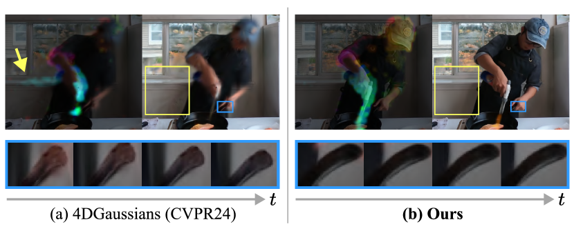
Figure 1: Overview. Existing field-based deformable 3D Gaussian Splatting methods predict Gaussian deformations at similar locations to be entangled. As a result, dynamic Gaussians influence adjacent static Gaussians, causing static regions to move along the nearby dynamic regions and exhibit degraded quality (left). Our model solves the problem by employing per-Gaussian latent embeddings to predict deformations for each Gaussian and achieves a clearer representation of dynamic motion (right).

1 Introduction

Dynamic scene reconstruction from multi-view input videos is an important task in computer vision, as it can be extended to various applications and industries such as mixed reality, content production, etc. Neural Radiance Fields (NeRF) [14], which enable photorealistic novel view synthesis from multi-view inputs, can represent dynamic scenes by modeling the scene with an additional time input [19, 10]. However, typical NeRFs require querying multilayer perceptron (MLP) for hundreds of points per camera ray, which limits rendering speed.

On the other hand, the recently emerging 3D Gaussian Splatting (3DGS) [8] has the advantage of real-time rendering compared to NeRFs using a differentiable rasterizer for 3D Gaussian primitives. 3DGS directly optimizes the parameters of 3D Gaussian (position, opacity, anisotropic covariance, and spherical harmonics (SH) coefficients) and renders them via projection and $\alpha$-blending. Since 3DGS has the characteristics of continuous volumetric radiance fields, some recent studies[25, 28, 3, 7, 12, 29] represent dynamic scenes by defining a canonical 3DGS and deforming it to individual frames as deformable NeRFs [28] do. Specifically, they model the deformation as a function of 4D (x, y, z, t) coordinates with MLPs or grids, i.e., fields, predicting the change in the 3D Gaussian parameters.

However, it is not appropriate to model the deformation of Gaussian parameters as a field for representing dynamic scenes because the positions of Gaussians change during optimization. Furthermore, nearby Gaussians tend to have similar deformations because the deformation function is piecewise continuous. As shown in Figure 1, the Gaussians in static regions, e.g., window, wall, and handle, are attracted by the motion of nearby dynamic objects. Moreover, the existing deformation-based approaches have an inherent property: all frames share a single canonical set of Gaussians. It makes the deformation hard to reconstruct different types or difficulties of movements in the dynamic scenes.

In this paper, we model the deformation of Gaussians at frames as 1) a function of a product space of per-Gaussian embeddings and temporal embeddings. We expect this rational design to bring quality improvement by precisely modeling different deformations of different Gaussians without interference due to adjacency. Additionally, 2) We decompose temporal variations of the parameters into coarse and fine components, namely coarse-fine deformation. The coarse deformation represents large or slow movements in the scene, while fine deformation learns the fast or detailed movements that coarse deformation does not cover. Finally, we propose 3) an efficient training strategy that samples difficult parts of the scene more frequently and facilitates the densification of Gaussians.

In our experiments, we observe that our per-Gaussian embeddings and coarse-fine deformation improve the deformation quality, while an efficient training strategy enables faster convergence. Additionally, our approach outperforms baselines in representing dynamic scenes, capturing fine details in dynamic regions, and excelling even under challenging camera settings.

2 Related Work

In this section, we review methods for dynamic scene reconstruction that deforms 3D canonical space and methods for reconstructing dynamic scenes utilizing dynamic 3D Gaussians. Afterward, we review the methods using embedding and efficient sampling techniques.

2.0.1 Deforming 3D Canonical Space

D-NeRF[19] reconstructs dynamic scenes by deforming ray samples over time, using the deformation network that takes 3D coordinates and timestamps of the sample as inputs. Nerfies[16] and HyperNeRF[17] use per-frame trainable deformation codes instead of time conditions to deform the canonical space. Instead of deforming from the canonical frame to the entire frames, HyperReel[1] deforms the ray sample of the keyframe to represent the intermediate frame. 4DGaussians [25] and D3DGS [28] reconstruct the dynamic scene with a deformation network which inputs the center position of the canonical 3D Gaussians and timestamps. In contrast, we demonstrate a novel deformation scheme to represent the deformation as a function of a product space of per-Gaussian latent embeddings and temporal embeddings.

2.0.2 Dynamic 3D Gaussians

To extend the fast rendering speed of 3D Gaussian Splatting[8] into dynamic scene reconstructions. 4DGaussians[25] decodes features from multi-resolution HexPlanes for temporal deformation of 3D Gaussians. While D3DGS[28] uses an implicit function that processes the time and location of the Gaussian. 4DGS[26] decomposed the 4D Gaussians into a time-conditioned 3D Gaussians and a marginal 1D Gaussians. STG[11] represents changes in 3D Gaussian over time through a temporal opacity and a polynomial function for each Gaussian.

Our method uses deformable 3D Gaussians as 4DGaussians[25] and D3DGS[28] do, but does not necessitate the separated feature field to obtain the input feature of the deformation decoder. Our approach uses embedding allocated to each Gaussian and a temporal embedding shared within a specific frame.

2.0.3 Latent Embedding on Novel View Synthesis

Some studies incorporate latent embeddings to represent different states of the static and dynamic scene. NeRF-W[13] and Block-NeRF[22] employ per-image appearance embeddings to capture different states of a scene, representing the dynamic scenes from in-the-wild image collections. DyNeRF and MixVoxels[10, 23] employ a temporal embedding for each frame to represent dynamic scenes. Nerfies[16] and HyperNeRF[17] incorporate both per-frame appearance and deformation embeddings. Sync-NeRF[9] introduces time offset to calibrate the misaligned temporal embeddings on dynamic scenes from unsynchronized videos. We introduce per-Gaussian latent embedding to encode the changes over time of each Gaussian, and use temporal embeddings to represent different states in each frame of the scene.

2.0.4 Efficient Training Strategy

To accelerate convergence and enhance performance, ActiveNeRF[15] selects the view by reducing the uncertainty of the input views. DS-NeRF and TermiNeRF[2, 18] samples the points with the sampling network. In the dynamic scene reconstruction, DyNeRF[10] samples rays over time, calculating he weight of each ray based on the residual difference between its color across time. STG[11] samples additional Gaussians along the ray within patches exhibiting significant errors. On the other hand, we present a simple view sampling method through pairwise camera distances, for the first time, we present a sampling method for a target training frame.

3 Method

In this section, we first provide a brief overview of 3D Gaussian Splatting (Section 3.1). Next, we introduce our overall framework, embedding-based deformation for Gaussians (Section 3.2) and coarse-fine deformation scheme consisting of coarse and fine deformation functions (Section 3.3). Finally, we present an efficient training strategy for faster convergence and higher performance (Section 3.4).

3.1 Preliminary: 3D Gaussian Splatting

3D Gaussian splatting[8] optimizes a set of anisotropic 3D Gaussians through differentiable tile rasterization to reconstruct a static 3D scene. By its efficient rasterization, the optimized model enables real-time rendering of high-quality images. Each 3D Gaussian function $G_{i}(x)$ at the point $x$ consist with position $\mathbf{x}_{i}$, rotation $R_{i}$, and scale $S_{i}$:.

$$G_{i}(x)=e^{-\frac{1}{2}(x-\mathbf{x}_{i})^{T}\Sigma_{i}^{-1}(x-\mathbf{x}_{i})},\qquad where\quad\Sigma_{i}=R_{i}S_{i}S_{i}^{T}R_{i}^{T}.$$ (1)

To projecting 3D Gaussians to 2D for rendering, covariance matrix $\Sigma^{\prime}$ are calculated by viewing transform $W$ and the Jacobian $J$ of the affine approximation of the projective transfomation[31] as follows:

$$\Sigma^{\prime}=JW\Sigma W^{T}J^{T}$$ (2)

Blending $\mathcal{N}$ depth-ordered projected points that overlap the pixel, the Gaussian function $G_{i}(x)$ is multiplied by the opacity of the Gaussian $\sigma_{i}$ and calculates the pixel color $C$ with the color of the Gaussian $c_{i}$:

$$C=\sum_{i\in\mathcal{N}}c_{i}\alpha_{i}\prod_{j=1}^{i-1}(1-\alpha_{j}),\qquad where\quad\alpha_{i}=\sigma_{i}G_{i}(x).$$ (3)

The color of Gaussian $c_{i}$ is determined using the SH coefficient with view direction.

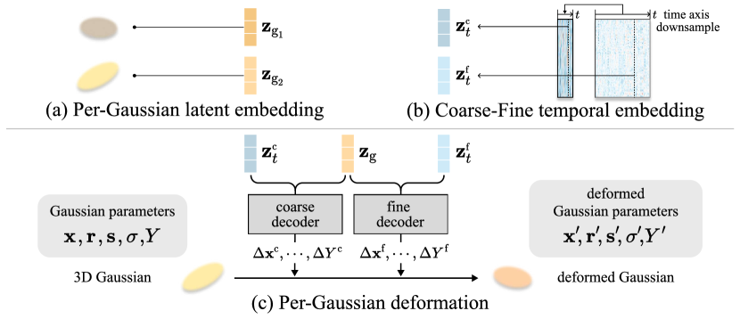
Figure 2: Framework. Existing field-based deformation methods suffer from the entanglement of nearby Gaussians as they map the changes of deformation parameters from Gaussian coordinates. To this end, we define per-Gaussian deformation. (a) Firstly, we assign a latent embedding for each Gaussian. (b) Additionally, we introduce coarse and fine temporal embeddings to represent the slow and fast state of the dynamic scene. (c) By employing two decoders that take per-Gaussian latent embeddings along with coarse and fine temporal embeddings as input, we estimate slow or large changes and fast or detailed changes to model the final deformation, respectively.

3.2 Embedding-Based Deformation for Gaussians

Deformable NeRFs consist of a deformation field that predicts displacement $\Delta\mathbf{x}$ for a given coordinate $\mathbf{x}$ from the canonical space to each target frame, and a radiance field that maps color and density from a given coordinate in the canonical space ($\mathbf{x}+\Delta\mathbf{x}$). Existing deformable Gaussian methods employ the same approach for predicting the deformation of Gaussians, i.e., utilizing a deformation field based on coordinates.

Unlike previous methods, we start from the design of 3DGS: the 3D scene is represented as a mixture of Gaussians that have individual radiance fields. Accordingly, the deformation should be defined for each Gaussian. Based on this intuition, we introduce a function $\mathcal{F}_{\theta}$ that produces deformation from learnable embeddings $\mathbf{z}_{\text{g}}\in\mathbb{R}^{32}$ belonging to individual Gaussians (Figure 2a), and typical temporal embeddings $\mathbf{z}_{t}\in\mathbb{R}^{256}$ for different frames:

$$\mathcal{F}_{\theta}:(\mathbf{z}_{\text{g}},\mathbf{z}_{t})\rightarrow(\Delta\mathbf{x},\Delta\mathbf{r},\Delta\mathbf{s},\Delta\sigma,\Delta Y),$$ (4)

where $\mathbf{r}$ is a rotation quaternion, $\mathbf{s}$ is a vector for scaling, $\sigma$ is an opacity, and $Y$ is SH coefficients for modeling view-dependent color. We implement $\mathcal{F}_{\theta}$ as a shallow multi-layer perceptron (MLP) followed by an MLP head for each parameter. As a result, the Gaussian parameters at frame $t$ are determined by adding $\mathcal{F}_{\theta}(\mathbf{z}_{\text{g}},\mathbf{z}_{t})$ to the canonical Gaussian parameters (Figure 2c).

We jointly optimize the per-Gaussian embeddings $\mathbf{z}_{\text{g}}$, the deformation function $\mathcal{F}_{\theta}$, and the canonical Gaussian parameters to minimize rendering loss. We use the L1 and periodic DSSIM as the rendering loss between the rendered image and the ground truth image.

3.3 Coarse-Fine Deformation

Different parts of a scene may have coarse and fine motions [5]. E.g., a hand swiftly stirs a pan (fine) while a body slowly moves from left to right (coarse). Based on this intuition, we introduce a coarse-fine deformation that produces a summation of coarse and fine deformations.

Coarse-fine deformation consists of two functions with the same architecture: one for coarse and one for fine deformation (Figure 2c). The functions receive different temporal embeddings as follows:

Following typical temporal embeddings, we start from a 1D feature grid $Z\in\mathbb{R}^{N\times 256}$ for $N$ frames and use an embedding $\mathbf{z}_{t}^{{}_{\text{f}}}=\text{interp}(Z,t)$ for fine deformation. For coarse deformation, we linearly downsample $Z$ by a factor of 5 to remove high-frequencies responsible for fast and detailed deformation. Then we compute $\mathbf{z}_{t}^{{}_{\text{c}}}$ as a linear interpolation of embeddings at enclosing grid points (Figure 2b).

As a result, coarse deformation $\mathcal{F}_{\theta_{\text{c}}}$($\mathbf{z}_{\text{g}}$, $\mathbf{z}_{t}^{{}_{\text{c}}}$) is responsible for representing large or slow movements in the scene, while fine deformation $\mathcal{F}_{\theta_{\text{f}}}$($\mathbf{z}_{\text{g}}$, $\mathbf{z}_{t}^{{}_{\text{f}}}$) learns the fast or detailed movements that coarse deformation does not cover. This improves the deformation quality. Refer to the Ablation study section for more details.

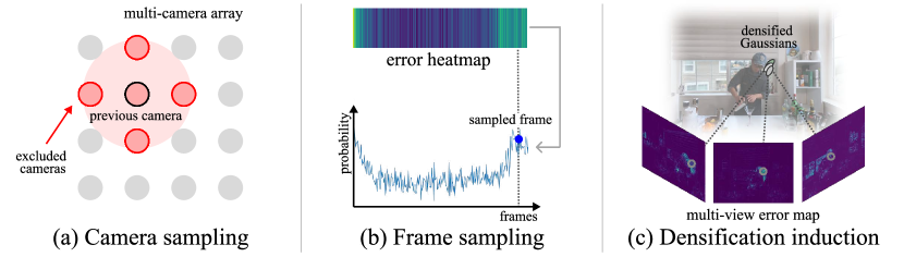
Figure 3: Components of efficient training strategy. (a) To ensure the diversity in camera viewpoints, we exclude the cameras close to the center of the previous camera from the next sampling. (b) We record the L1 error between the rendered image and ground truth during training, which is used to generate a probability distribution for frame sampling, focusing on frames with higher errors. (c) We periodically add the multi-view DSSIM loss to induce Gaussian densification in challenging regions.

3.4 Efficient Training Strategy

Last but not least, we introduce a training strategy for faster convergence and higher performance. The first is to evenly cover multi-view camera perspectives and exclude the camera index that was used in the previous iteration. We pre-compute pairwise distances of all camera origins before the start of the training. Then we exclude the cameras with distance to the previous camera less than 40 percentile of all distances.

The second is to sample frames within the target cameras. Different frames may have different difficulties for reconstruction. We measure the difficulty of a frame by the magnitude of error at the frame. Then, we sample training frames with a categorical distribution which is proportional to the magnitude of error. For multi-view videos, we average the errors from all viewpoints. We use this sampling every other iteration with random sampling.

The third is to change the policy for Gaussian densification. Previous methods invoke the densification by minimizing L1 loss [25] or L1 loss and DSSIM loss for every iteration [27, 28, 11]. We observe that the DSSIM loss improves the visual quality in the background but takes longer training time. Therefore, we use L1 loss for every iteration and periodically use the additional multi-view DSSIM loss in the frame with high error. This encourages densification in the region where the model struggles (See Section 0.A.1).

4 Experiment

In this section, we first describe the criterion for selection of baselines, and evaluation metrics. We then demonstrate the effectiveness of our method through comparisons with various baselines and datasets (Section 4.1-4.2). Finally, we conduct analysis and ablations of our method (Section 4.3).

4.0.1 Baselines

We choose the start-of-the-art method as a baseline in each datasets. We compared against DyNeRF, NeRFPlayer, MixVoxels, K-Planes, HyperReel, Nerfies, HyperNeRF, and TiNeuVox on the NeRF baseline. In detail, we use the version of NeRFPlayer TensoRF VM, HyperNeRF DF, Mixvoxels-L, K-Planes hybrid. We compared with 4DGaussians, 4DGS, and D3DGS based on the Gaussian baseline. Meanwhile, we have not included STG in our comparison due to its requirement for per-frame Structure from Motion (SfM) points, which makes conducting a fair comparison challenging. Also, STG is not a deformable 3D Gaussian approach. We followed the official code and configuration, except increasing the training iterations for the Technicolor dataset to 1.5 times that of the 4DGaussians, in comparison to the Neural 3D Video dataset.

4.0.2 Metrics

We report the quality of rendered images using PSNR, SSIM, and LPIPS. Peak Signal-to-Noise Ratio (PSNR) quantifies pixel color error between the rendered video and the ground truth. We utilize SSIM [24] to account for the perceived similarity of the rendered image. Additionally, we measure higher-level perceptual similarity using Learned Perceptual Image Patch Similarity (LPIPS) [30] with an AlexNet Backbone. Higher PSNR and SSIM values and lower LPIPS values indicate better visual quality.

Figure 4: Qualitative comparisons on the Neural 3D Video Dataset. The baseline models exhibit blurriness or artifacts in dynamic areas such as hands and torches, whereas ours successfully reconstructs them.

4.1 Effectiveness on dynamic region

4.1.1 Neural 3D Video Dataset

[10] includes 20 multi-view videos, with each scene consisting of either 300 frames, except for the flame_salmon scene, which comprises 1200 frames. These scenes encompass a relatively long duration and various movements, with some featuring multiple objects in motion. We utilized Neural 3D Video dataset to observe the capability to capture dynamic areas. Total six scenes (coffee_martini, cook_spinach, cut_roasted_beef, flame_salmon, flame_steak, sear_steak) are evaluated in Figure 4 and Table 1. The flame_salmon scene divided into four segments, each containing 300 frames.

Figure 4 reports the rendering quality. Our method successfully reconstructs the fine details in moving areas, outperforming baselines on average metrics across test views. Baselines show blurred dynamic areas or severe artifacts in low-light scenes such as cook_spinach and flame_steak. 4DGS exhibits the disappearance of some static areas. In 4DGaussians, a consistent over-smoothing occurs in dynamic areas. All baselines experienced reduced quality in reflective or thin dynamic areas like clamps, torches, and windows.

Table 1 presents quantitative metrics on the average metrics across the test views of all scenes, computational and storage costs on the first fragment of flame_salmon scene. Refer to the Appendix for per-scene details. Our method demonstrates superior reconstruction quality across all metrics compared to baselines. As the table shows, NeRF baselines generally required longer training and rendering times. While 4DGS shows relatively high reconstruction performance, it demands longer training times and larger VRAM storage capacity compared to other baselines. 4DGaussians requires lower computational and storage cost but it displays low reconstruction quality in some scenes with rapid dynamics, as shown in the teaser and Figure 4.

Table 1: Average performance in the test view on Neural 3D Video Dataset The computational cost was measured based on flame_salmon_1 on the A6000. ¹flame salmon scene includes only the first segment, comprising 300 frames. ²reported time and DyNeRF is trained on 8 GPUs and tested only on flame salmon. ³trained with 90 frames. ⁴trained with 50 frames.

model	metric			computational cost
	PSNR$\uparrow$	SSIM$\uparrow$	LPIPS$\downarrow$	Training time$\downarrow$	FPS$\uparrow$	Model size$\downarrow$
DyNeRF12 [10]	29.58	-	0.083	1344 hours	0.01	56 MB
NeRFPlayer13 [21]	30.69	-	0.111	6 hours	0.05	1654 MB
MixVoxels [23]	30.30	0.918	0.127	1 hours 40 mins	0.93	512 MB
K-Planes [6]	30.86	0.939	0.096	1 hours 40 mins	0.13	309 MB
HyperReel4 [1]	30.37	0.921	0.106	9 hours 20 mins	1.0	1362 MB
4DGS [26]	31.19	0.940	0.051	9 hours 30 mins	33.7	8700 MB
4DGaussians [25]	30.71	0.935	0.056	50 mins	51.9	59 MB
Ours	31.42	0.945	0.037	3 hours 35 mins	19.9	137 MB

4.1.2 Technicolor Light Field Dataset

[20] is a multi-view dataset captured with a time-synchronized $4\times 4$ camera rig, containing intricate details. We train ours and the baselines on 50 frames of five commonly used scenes (Birthday, Fabien, Painter, Theater, Trains) using full-resolution videos at $2048\times 1088$ pixels, with the second row and second column cameras used as test views.

As shown in Figure 5, HyperReel produces noisy artifacts due to incorrect predictions of the displacement vector. 4DGaussians fails to capture fine details in dynamic areas, exhibiting over-smoothing results. All baselines struggle to accurately reconstruct rapidly moving thin areas like fingers.

Table 2 reports the average metrics across the test views of all scenes, computational and storage costs on Painter scene. HyperReel demonstrates overall high-quality results but struggles with relatively slow training times and FPS, and a larger model size. 4DGaussians exhibits fast training times and FPS but significantly underperforms in reconstructing fine details compared to other baselines. However, our method demonstrates superior reconstruction quality and faster FPS compared to the baselines.

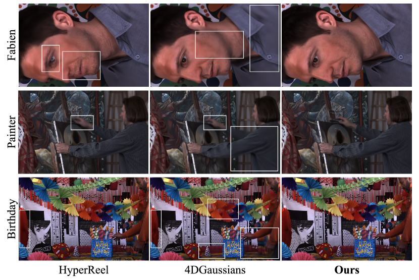
Figure 5: Qualitative comparisons on the Technicolor Dataset. HyperReel exhibits noise artifacts in specific frames or regions, and 4DGaussians fails to represent detailed textures in dynamic areas, while ours reconstructs dynamic areas and details in the scene well.

Table 2: Average performance in the test view on Technicolor Dataset

model	metric			computational cost
	PSNR$\uparrow$	SSIM$\uparrow$	LPIPS$\downarrow$	Training time$\downarrow$	FPS$\uparrow$	Model size$\downarrow$
DyNeRF	31.80	-	0.140	-	0.02	0.6 MB
HyperReel	32.32	0.899	0.118	2 hours 45 mins	0.91	289 MB
4DGaussians	29.62	0.844	0.176	25 mins	34.8	51 MB
Ours	33.38	0.907	0.103	1 hours 30 mins	36.5	56 MB

4.2 Scenes with Challenging Camera Setting

4.2.1 HyperNeRF dataset

includes videos using two Pixel 3 phones rigidly mounted on a handheld capture rig. We train on all frames of four scenes (3D Printer, Banana, Broom, Chicken) at a resolution downsampled by a factor of two to $536\times 960$. Due to memory constraints, D3DGS is trained on images further downsampled to a quarter of their original size.

Figure 6 shows that the previous methods struggle to reconstruct fast-moving parts such as fingers and broom. Especially D3DGS deteriorates in Broom. Table 3 reports the average metrics across the test views of all scenes, computational and storage costs on Broom scene. The table shows that our method outperforms the reconstruction performance with previous methods along with compact model size and faster FPS.

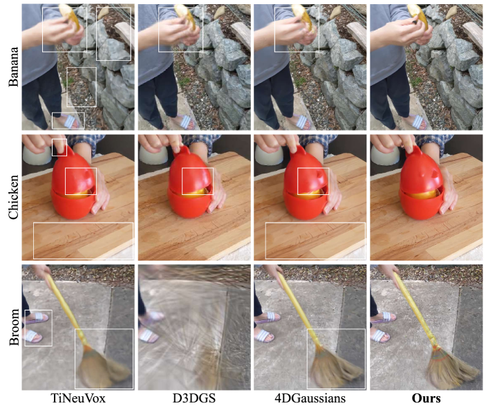
Figure 6: Qualitative comparisons on the HyperNeRF Dataset. Previous methods struggle slightly with reconstructing fast-moving parts, as evidenced by the boxed area in the image.

Table 3: Average performance in the test view on Hypernerf Dataset

model	metric			computational cost
	PSNR$\uparrow$	SSIM$\uparrow$	LPIPS$\downarrow$	Training time$\downarrow$	FPS$\uparrow$	Model size$\downarrow$
Nerfies [16]	22.23	-	0.170	$\sim$ hours	$<$ 1	-
HyperNeRF DS [17]	22.29	0.598	0.153	32 hours	$<$ 1	15 MB
TiNeuVox [4]	24.20	0.616	0.393	3 hours 30 mins	1	48 MB
D3DGS [28]	22.40	0.598	0.275	16 mins	6.95	309 MB
4DGaussians	25.03	0.682	0.281	50 mins	96.3	60 MB
Ours	25.53	0.694	0.242	1 hours 20 mins	30.9	34 MB

4.3 Analyses and Ablation Study

4.3.1 Improving Rendering Speed

Our method can enhance rendering speed by omitting the deformation of Gaussians in static areas, which only require a single computation of parameter changes from the canonical space. To identify static Gaussians, we sum up the L1 norms of each Gaussian parameter over time and select Gaussians below the $k$ percentile based on the aggregated value. As Table 4 reports, we can obtain almost identical rendering quality to the original, despite omitting decoder evaluations for 90% of the total Gaussian. The experiments are conducted on flame_salmon_1 scene with a single NVIDIA RTX 4090.

Table 4: Quantitative comparison of skip deformation. By omitting redundant evaluation for static Gaussians, ours achieves faster rendering speed with almost the same performance.

Skip deformation	PSNR$\uparrow$	SSIM$\uparrow$	LPIPS$\downarrow$	FPS$\uparrow$
0% (original)	29.72	0.935	0.038	17.1
50%	29.72	0.935	0.038	25.7
70%	29.72	0.935	0.038	26.0
90%	29.68	0.935	0.038	28.4

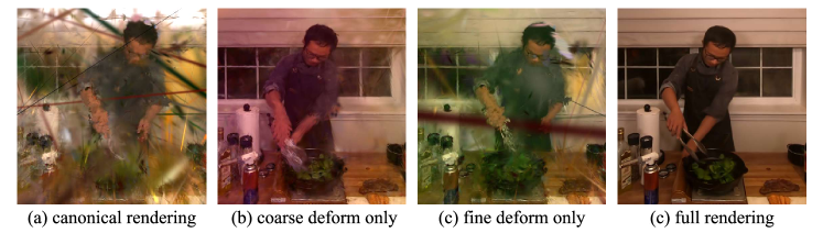
Figure 7: Deformation components. (a) The canonical space contains Gaussians to represent all target frames of the scene. (b) Applying coarse deformation to the canonical space roughly reflects the dynamics of the scene. (c) The rendering without coarse deformation and only with fine deformation looks similar to the canonical rendering. (d) Applying both coarse and fine deformation yields natural rendering results.

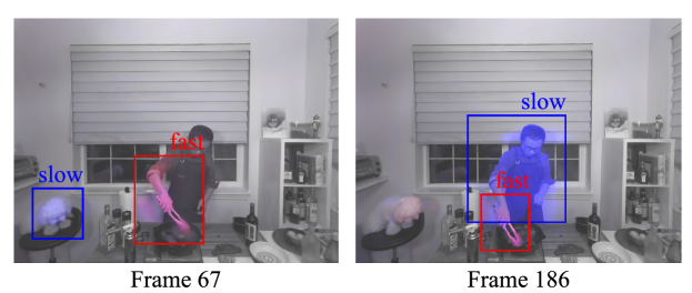
Figure 8: Visualization of the magnitude of deformation. Coarse deformation (blue) captures large and slow changes, such as the movement of the head and torso, while fine deformation (red) is responsible for the fast and detailed movements of arms, tongs, shadows, etc.

4.3.2 Deformation components

In Figure 7, we present an analysis of the coarse-fine deformation. To achieve this, we render a flame_steak scene by omitting each of our deformation components one by one. Our full rendering results from adding coarse and fine deformation to the canonical space (Figure 7d). When both are removed, rendering yields an image in canonical space (Figure 7a). Rendering with the coarse deformation, which handles large or slow changes in the scene, produces results similar to the full rendering (Figure 7b). On the other hand, fine deformation is responsible for fast or detailed changes in the scene, yielding rendering similar to canonical space (Figure 7c).

To examine the roles of the coarse and fine deformation in the coarse-fine deformation, we conduct a visualization on flame_steak scene. First, we compute the Euclidean norm of positional shifts between the current and subsequent frames. We then add the value to the DC components of the SH coefficients proportionally to the magnitude: blue for coarse deformation and red for fine deformation. For visual clarity, we render the original scene in grayscale. As illustrated in Figure 8, coarse deformation models slower changes such as body movement, while fine deformation models faster movements like cooking arms. Thus, we demonstrate that by downsampling the temporal embedding grid $Z$, we can effectively separate and model slow and fast deformations in the scene.

Table 5: Ablation study of proposed methods. We compare the rendering results of checkpoints at 30K iterations on the flame_salmon_4 scene.

Method	PSNR $\uparrow$	SSIM $\uparrow$	LPIPS $\downarrow$
Ours Full	29.08	0.924	0.056
w/o Coarse-Fine deformation	28.74	0.922	0.060
w/o Efficient training strategy	28.89	0.920	0.056

Table 6: Quantitative comparison of ablation study. Training our model without coarse deformation or fine deformation results in degraded performance. Furthermore, including center coordinates of Gaussian as additional inputs to the decoder significantly reduces performance.

Method	PSNR$\uparrow$	SSIM$\uparrow$	LPIPS$\downarrow$
Ours Full	30.28	0.934	0.047
coarse deformation only	29.71	0.930	0.050
fine deformation only	29.62	0.929	0.048
Ours + $\mathbf{x}$ injection	28.17	0.916	0.057

4.3.3 Ablation study

To verify the effectiveness of each component of our method, we report the performance when each component is removed. To observe the impact of the coarse-fine deformation, we train a total of 100K iterations on flame_salmon_4 scene. To show the efficiency of our training strategy, we evaluate the rendering results from checkpoints of 30K iterations. As shown in Table 5, we confirm that the performance decreases when each component is removed.

Furthermore, we report the results of an ablation study on the deformation decoder in Figure 9 and Table 6. First, our full method (using both coarse and fine decoders) produces clear rendering results and models dynamic variations well (Figure 9a). Training only with the coarse decoder leads to blurred dynamic areas and a failure to accurately capture detailed motion (Figure 9)b. On the other hand, only with the fine decoder, the model results in small floats and noisy rendering in the dynamic regions (Figure 9c).

Additionally, we demonstrate experiments where the Gaussian center coordinates $\mathbf{x}$ are injected into the input of each decoder. As shown in 9d, including the Gaussian coordinates not only degrades the quality of deformation but also reduces the quality of static background areas, supporting our argument that coordinate dependency should be removed from the deformation function.

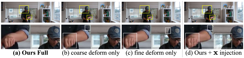
Figure 9: Qualitative comparison of ablation study. We use flame_salmon_4 scene for ablation study of deformation decoder. (a) Our model achieves clear results with both coarse and fine decoders. (b-c) The quality of dynamic areas decreases if one is missing. (d) Additionally, introducing the coordinates of Gaussian as an additional input into our decoders results in a decrease in the quality of both static and dynamic regions.

5 Conclusion and Limitation

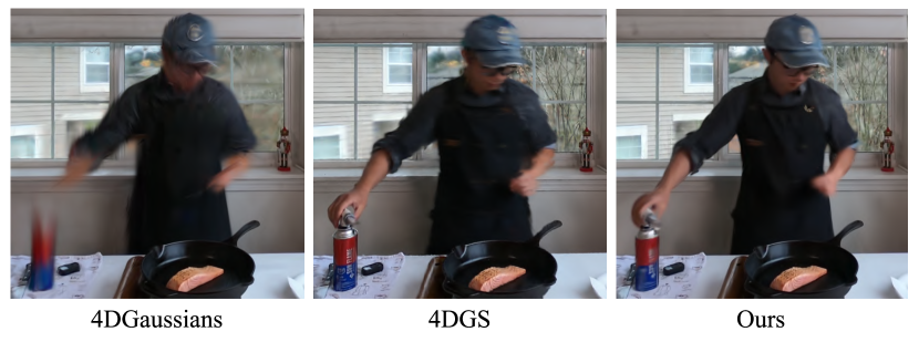
Figure 10: Limitation. Our model is not completely free from blurriness in fast motion as in the baselines.

We propose a per-Gaussian deformation for 3DGS that takes per-Gaussian embeddings as input instead of using the typical deformation field of deformable 3DGS methods, achieving high performance. We enhance the quality by decomposing the dynamic changes into coarse and fine deformation. However, our method also has limitations. The dynamic regions of our rendering results tend to be blurred when there is significant motion between frames, as in the other baselines (Figure 10). It is expected to be resolved with additional supervision like correspondences in rapidly changing dynamic regions. In addition, our method tends to be slower in rendering compared to existing Gaussian Splatting methods. This could be improved by skipping the deformation prediction for static areas and pruning unnecessary points after training, as mentioned before.

In Appendix, we first provide a more detailed analysis of our method (Appendix 0.A). We then provide the additional training details(Appendix 0.B), and the per-scene quantitative and qualitative results on all datasets (Appendix 0.C).

Appendix 0.A More Analysis

0.A.1 Effect of multi-view DSSIM loss

Figure S1: Multi-View DSSIM loss. We present the background region and the overall training time on flame_salmon_1 scene. Our approach requires a reasonable additional computational cost while improving the reconstruction quality, compared to training without the use of DSSIM loss.

As shown in Figure S1, we observe that DSSIM loss helps to learn difficult areas in the scene, such as the details of the background. However, optimizing DSSIM loss at every step [8] is computationally expensive, and the introduction of DSSIM loss increases the number of Gaussians, further extending the training time. Our multi-view DSSIM loss achieves a similar level of quality to what is computed at every step while reducing the number of computations for DSSIM.

0.A.2 Effect of embedding size

Table S1: Ablation study on the size of temporal and per-Gaussian embeddings. We compare the results on the flame_steak scene. Our default setting is shown in bold.

$\mathbf{z}_{t}$ dim/$\mathbf{z}_{\text{g}}$ dim	PSNR $\uparrow$	SSIM $\uparrow$	LPIPS $\downarrow$	$\mathbf{z}_{t}$ dim/$\mathbf{z}_{\text{g}}$ dim	PSNR $\uparrow$	SSIM $\uparrow$	LPIPS $\downarrow$
256 / 16	32.79	0.960	0.030	128 / 32	33.23	0.962	0.028
256 / 32	33.28	0.963	0.028	256 / 32	33.28	0.963	0.028
256 / 64	32.60	0.960	0.031	512 / 32	32.80	0.961	0.031

We report the performance variation by changing the size of per-Gaussian and temporal embeddings in Table S1. We observe that the model is sensitive to the size of $\mathbf{z}_{\text{g}}$ while it is less sensitive to the size of $\mathbf{z}_{t}$. We choose the dimensions of $\mathbf{z}_{\text{g}}$ and $\mathbf{z}_{t}$ to be 32 and 256, respectively.

Appendix 0.B Training Details

0.B.1 Details of Efficient Training Strategy

For camera sampling, we exclude cameras close to the previous camera center for the next sampling candidates. This is achieved by calculating the pairwise distance between all camera origin and excluding the cameras below the 40 percentile of distances.

For frame sampling, we record the L1 error between rendered images and ground truth for each frame during training. We treat this as a probability distribution for frame sampling to focuse on frames with higher errors. For the first 10K iterations, we randomly sample the frames, and then alternately use random sampling and error-based frame sampling.

Finally, we use multi-view DSSIM loss with L1 loss to induce densification in areas where the model struggles, such as background or dynamic regions. Due to the computational cost of SSIM, we fix the frame obtained by loss-based sampling for every 50 iterations, and minimize the multi-view DSSIM loss through camera sampling during the next 5 iterations. Similar to frame sampling, DSSIM loss is applied after the first 10K iterations.

0.B.2 Implementation Details

In all experiments, we use a 32-dimensional vector for Gaussian embeddings $\mathbf{z}_{\text{g}}$ and a 256-dimensional vector for temporal embeddings $\mathbf{z}_{t}$. The decoder MLP consists 128 hidden units and the MLP head for Gaussian parameters are both composed of 2 layers with 128 hidden units. For Technicolor and HyperNeRF datasets, we use a 1-layer decoder MLP. To efficiently and stabilize the initial training, we start the temporal embedding grid $Z_{t}^{\text{f}}$ at the same $N/5$ time resolution as $Z_{t}^{\text{c}}$ and gradually increase it to $N$ resolution over 10K iterations, with $N$ set to 150 for 300 frames. The learning rate of our deformation decoder starts at $1.6\times 10^{-4}$ and exponentially decays to $1.6\times 10^{-5}$ over the total training iterations. The learning rate of the temporal embedding $\mathbf{z}_{t}$ follows that of the deformation decoder, while the learning rate of per-Gaussian embedding $\mathbf{z}_{\text{g}}$ is set to $2.5\times 10^{-3}$. We eliminate the opacity reset step of 3DGS and instead add a loss that minimizes the mean of Gaussian opacities with a weight of $1.0\times 10^{-4}$. We empirically set the start of the training strategy to 10K iterations. Following Sync-NeRF, we introduce a learnable time offset to each camera in Neural 3D Video and Technicolor Light Field dataset.

For initialization points, we downsample point clouds obtained from COLMAP dense scene reconstruction. For Neural 3D Video dataset, we train for 80K iterations; for Technicolor dataset, 100K for the Birthday and Painter scenes and 120K for the rest; for the HyperNeRF dataset, 80K for the banana scene and 60K for the others. We periodically use the DSSIM loss at specific steps, excluding the HyperNeRF dataset. For calculating computational cost, the Neural 3D Video dataset was measured using A6000, while the Technicolor Light Field Dataset and the HyperNeRF Dataset were measured using 3090.

Appendix 0.C More Results

Table S2-S4 report the quantitative results of each scene on Neural 3D Video Dataset, Technicolor Light Field Dataset, and HyperNeRF Dataset. In most scenes, our model shows better perceptual performance than the baselines. Additionally, we show the entire rendering results in Figure S2-S4.

0.C.1 Per-Scene Results of Neural 3D Video Dataset

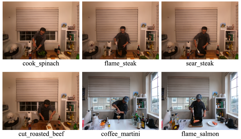
Figure S2: Rendering results on Neural 3D Video Dataset.

Table S2: Per-scene quantitative results on Neural 3D Video dataset

	Average		coffee_martini		cook_spinach		cut_roasted_beef		flame_salmon_1
	PSNR$\uparrow$	SSIM$\uparrow$	PSNR$\uparrow$	SSIM$\uparrow$	PSNR$\uparrow$	SSIM$\uparrow$	PSNR$\uparrow$	SSIM$\uparrow$	PSNR$\uparrow$	SSIM$\uparrow$
MixVoxels	30.30	0.918	29.44	0.916	29.97	0.934	32.58	0.938	30.50	0.918
K-Planes	30.86	0.939	29.66	0.926	31.82	0.943	31.82	0.966	30.68	0.928
HyperReel	30.37	0.921	28.37	0.892	32.30	0.941	32.92	0.945	28.26	0.882
4DGS	30.71	0.935	28.44	0.919	33.10	0.953	33.32	0.954	28.80	0.906
4DGaussians	31.19	0.940	28.63	0.918	33.54	0.956	34.18	0.959	29.25	0.929
Ours	31.42	0.945	29.33	0.931	33.19	0.957	33.25	0.957	29.72	0.935
	flame_salmon_2		flame_salmon_3		flame_salmon_4		flame_steak		sear_steak
	PSNR$\uparrow$	SSIM$\uparrow$	PSNR$\uparrow$	SSIM$\uparrow$	PSNR$\uparrow$	SSIM$\uparrow$	PSNR$\uparrow$	SSIM$\uparrow$	PSNR$\uparrow$	SSIM$\uparrow$
MixVoxels	30.53	0.915	27.83	0.853	29.49	0.899	30.74	0.945	31.61	0.949
K-Planes	29.98	0.924	30.10	0.924	30.37	0.922	31.85	0.969	31.48	0.951
HyperReel	28.80	0.911	28.97	0.911	28.92	0.908	32.20	0.949	32.57	0.952
4DGS	28.21	0.913	28.68	0.917	28.45	0.913	33.55	0.961	34.02	0.963
4DGaussians	29.28	0.929	29.40	0.927	29.13	0.925	33.90	0.961	33.37	0.960
Ours	29.76	0.931	30.12	0.935	30.28	0.934	33.55	0.963	33.55	0.963

0.C.2 Per-Scene Results of Technicolor Light Field Dataset

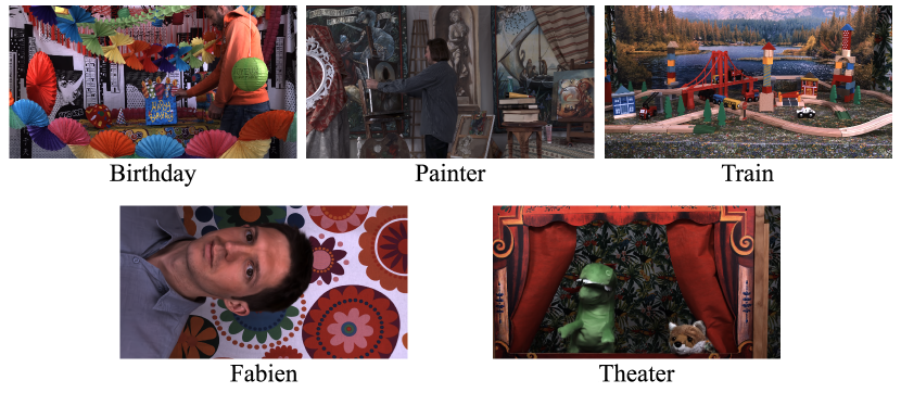
Figure S3: Rendering results on Technicolor Light Field Dataset.

Table S3: Per-scene quantitative results on Technicolor Dataset

	Average		Birthday		Fabien
	PSNR$\uparrow$	SSIM$\uparrow$	PSNR$\uparrow$	SSIM$\uparrow$	PSNR$\uparrow$	SSIM$\uparrow$
DyNeRF	31.80	-	29.20	-	32.76	-
HyperReel	32.32	0.899	30.57	0.918	32.49	0.863
4DGaussians	29.62	0.840	28.03	0.862	33.36	0.865
Ours	33.38	0.907	33.34	0.951	34.45	0.875
	Painter		Theater		Train
	PSNR$\uparrow$	SSIM$\uparrow$	PSNR$\uparrow$	SSIM$\uparrow$	PSNR$\uparrow$	SSIM$\uparrow$
DyNeRF	35.95	-	29.53	-	31.58	-
HyperReel	35.51	0.924	33.76	0.897	29.30	0.894
4DGaussians	34.52	0.899	28.67	0.835	23.54	0.756
Ours	36.63	0.923	30.64	0.864	31.84	0.922

0.C.3 Per-Scene Results of HyperNeRF Dataset

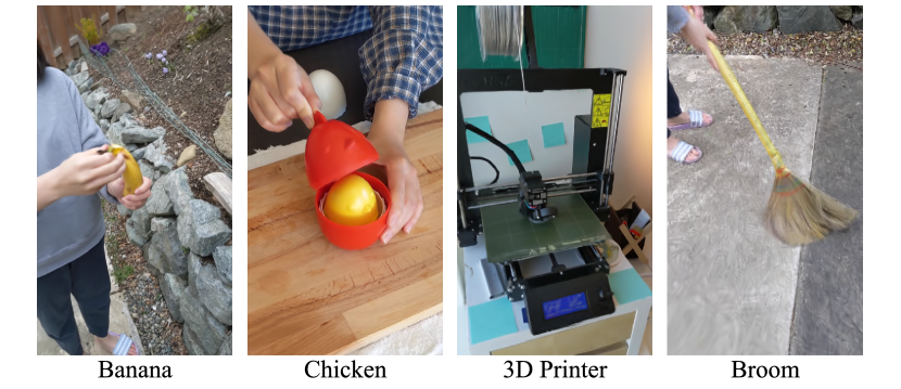
Figure S4: Rendering results on HyperNeRF Dataset.

Table S4: Per-scene quantitative results on HyperNeRF Dataset

	Average		Broom		3D Printer		Chicken		Banana
	PSNR$\uparrow$	SSIM$\uparrow$	PSNR$\uparrow$	SSIM$\uparrow$	PSNR$\uparrow$	SSIM$\uparrow$	PSNR$\uparrow$	SSIM$\uparrow$	PSNR$\uparrow$	SSIM$\uparrow$
Nerfies	22.23	-	19.3	-	20.00	-	26.90	-	23.30	-
HyperNeRF DS	22.29	0.598	19.51	0.210	20.04	0.635	27.46	0.828	22.15	0.719
TiNeuVox	24.20	0.616	21.28	0.307	22.80	0.725	28.22	0.785	24.50	0.646
D3DGS	22.40	0.598	20.48	0.313	20.38	0.644	22.64	0.601	26.10	0.832
4DGaussians	25.03	0.682	22.01	0.367	21.99	0.705	28.47	0.806	27.28	0.845
Ours	25.53	0.694	21.97	0.371	22.36	0.709	29.02	0.831	28.77	0.866

References

- [1] Attal, B., Huang, J.B., Richardt, C., Zollhoefer, M., Kopf, J., O’Toole, M., Kim, C.: Hyperreel: High-fidelity 6-dof video with ray-conditioned sampling. In: Proceedings of the IEEE/CVF Conference on Computer Vision and Pattern Recognition. pp. 16610–16620 (2023)
- [2] Deng, K., Liu, A., Zhu, J.Y., Ramanan, D.: Depth-supervised NeRF: Fewer views and faster training for free. In: Proceedings of the IEEE/CVF Conference on Computer Vision and Pattern Recognition (CVPR) (June 2022)
- [3] Duisterhof, B.P., Mandi, Z., Yao, Y., Liu, J.W., Shou, M.Z., Song, S., Ichnowski, J.: Md-splatting: Learning metric deformation from 4d gaussians in highly deformable scenes. arXiv preprint arXiv:2312.00583 (2023)
- [4] Fang, J., Yi, T., Wang, X., Xie, L., Zhang, X., Liu, W., Nießner, M., Tian, Q.: Fast dynamic radiance fields with time-aware neural voxels. In: SIGGRAPH Asia 2022 Conference Papers (2022)
- [5] Feichtenhofer, C., Fan, H., Malik, J., He, K.: Slowfast networks for video recognition. In: Proceedings of the IEEE/CVF international conference on computer vision. pp. 6202–6211 (2019)
- [6] Fridovich-Keil, S., Meanti, G., Warburg, F.R., Recht, B., Kanazawa, A.: K-planes: Explicit radiance fields in space, time, and appearance. In: Proceedings of the IEEE/CVF Conference on Computer Vision and Pattern Recognition. pp. 12479–12488 (2023)
- [7] Huang, Y.H., Sun, Y.T., Yang, Z., Lyu, X., Cao, Y.P., Qi, X.: Sc-gs: Sparse-controlled gaussian splatting for editable dynamic scenes. arXiv preprint arXiv:2312.14937 (2023)
- [8] Kerbl, B., Kopanas, G., Leimkühler, T., Drettakis, G.: 3d gaussian splatting for real-time radiance field rendering. ACM Transactions on Graphics 42(4) (July 2023), https://repo-sam.inria.fr/fungraph/3d-gaussian-splatting/
- [9] Kim, S., Bae, J., Yun, Y., Lee, H., Bang, G., Uh, Y.: Sync-nerf: Generalizing dynamic nerfs to unsynchronized videos. arXiv preprint arXiv:2310.13356 (2023)
- [10] Li, T., Slavcheva, M., Zollhoefer, M., Green, S., Lassner, C., Kim, C., Schmidt, T., Lovegrove, S., Goesele, M., Newcombe, R., et al.: Neural 3d video synthesis from multi-view video. In: Proceedings of the IEEE/CVF Conference on Computer Vision and Pattern Recognition (2022)
- [11] Li, Z., Chen, Z., Li, Z., Xu, Y.: Spacetime gaussian feature splatting for real-time dynamic view synthesis. arXiv preprint arXiv:2312.16812 (2023)
- [12] Liang, Y., Khan, N., Li, Z., Nguyen-Phuoc, T., Lanman, D., Tompkin, J., Xiao, L.: Gaufre: Gaussian deformation fields for real-time dynamic novel view synthesis (2023)
- [13] Martin-Brualla, R., Radwan, N., Sajjadi, M.S.M., Barron, J.T., Dosovitskiy, A., Duckworth, D.: NeRF in the Wild: Neural Radiance Fields for Unconstrained Photo Collections. In: CVPR (2021)
- [14] Mildenhall, B., Srinivasan, P.P., Tancik, M., Barron, J.T., Ramamoorthi, R., Ng, R.: Nerf: Representing scenes as neural radiance fields for view synthesis. Communications of the ACM 65(1), 99–106 (2021)
- [15] Pan, X., Lai, Z., Song, S., Huang, G.: Activenerf: Learning where to see with uncertainty estimation (2022)
- [16] Park, K., Sinha, U., Barron, J.T., Bouaziz, S., Goldman, D.B., Seitz, S.M., Martin-Brualla, R.: Nerfies: Deformable neural radiance fields. ICCV (2021)
- [17] Park, K., Sinha, U., Hedman, P., Barron, J.T., Bouaziz, S., Goldman, D.B., Martin-Brualla, R., Seitz, S.M.: Hypernerf: A higher-dimensional representation for topologically varying neural radiance fields. arXiv preprint arXiv:2106.13228 (2021)
- [18] Piala, M., Clark, R.: Terminerf: Ray termination prediction for efficient neural rendering (2021)
- [19] Pumarola, A., Corona, E., Pons-Moll, G., Moreno-Noguer, F.: D-nerf: Neural radiance fields for dynamic scenes. arXiv preprint arXiv:2011.13961 (2020)
- [20] Sabater, N., Boisson, G., Vandame, B., Kerbiriou, P., Babon, F., Hog, M., Gendrot, R., Langlois, T., Bureller, O., Schubert, A., et al.: Dataset and pipeline for multi-view light-field video. In: Proceedings of the IEEE conference on computer vision and pattern recognition Workshops. pp. 30–40 (2017)
- [21] Song, L., Chen, A., Li, Z., Chen, Z., Chen, L., Yuan, J., Xu, Y., Geiger, A.: Nerfplayer: A streamable dynamic scene representation with decomposed neural radiance fields. IEEE Transactions on Visualization and Computer Graphics 29(5), 2732–2742 (2023)
- [22] Tancik, M., Casser, V., Yan, X., Pradhan, S., Mildenhall, B., Srinivasan, P.P., Barron, J.T., Kretzschmar, H.: Block-nerf: Scalable large scene neural view synthesis (2022)
- [23] Wang, F., Tan, S., Li, X., Tian, Z., Liu, H.: Mixed neural voxels for fast multi-view video synthesis. arXiv preprint arXiv:2212.00190 (2022)
- [24] Wang, Z., Bovik, A.C., Sheikh, H.R., Simoncelli, E.P.: Image quality assessment: from error visibility to structural similarity. IEEE transactions on image processing 13(4), 600–612 (2004)
- [25] Wu, G., Yi, T., Fang, J., Xie, L., Zhang, X., Wei, W., Liu, W., Tian, Q., Xinggang, W.: 4d gaussian splatting for real-time dynamic scene rendering. arXiv preprint arXiv:2310.08528 (2023)
- [26] Yang, Z., Yang, H., Pan, Z., Zhang, L.: Real-time photorealistic dynamic scene representation and rendering with 4d gaussian splatting. In: International Conference on Learning Representations (ICLR) (2024)
- [27] Yang, Z., Yang, H., Pan, Z., Zhu, X., Zhang, L.: Real-time photorealistic dynamic scene representation and rendering with 4d gaussian splatting. arXiv preprint arXiv:2310.10642 (2023)
- [28] Yang, Z., Gao, X., Zhou, W., Jiao, S., Zhang, Y., Jin, X.: Deformable 3d gaussians for high-fidelity monocular dynamic scene reconstruction. arXiv preprint arXiv:2309.13101 (2023)
- [29] Yu, H., Julin, J., Milacski, Z. ., Niinuma, K., Jeni, L.A.: Cogs: Controllable gaussian splatting (2023)
- [30] Zhang, R., Isola, P., Efros, A.A., Shechtman, E., Wang, O.: The unreasonable effectiveness of deep features as a perceptual metric. In: Proceedings of the IEEE conference on computer vision and pattern recognition. pp. 586–595 (2018)
- [31] Zwicker, M., Pfister, H., Van Baar, J., Gross, M.: Surface splatting. In: Proceedings of the 28th annual conference on Computer graphics and interactive techniques. pp. 371–378 (2001)