Beyond the blur: using experimental point spread functions to help scanning Kelvin probe microscopy reach its full potential

Abstract

Scanning Kelvin probe microscopy (SKPM) is a powerful technique for investigating the electrostatic properties of material surfaces, enabling the imaging of variations in work function, topology, surface charge density, or combinations thereof. Regardless of the underlying signal source, SKPM results in a voltage image which is spatially distorted due to the finite size of the probe, long-range electrostatic interactions, mechanical and electrical noise, and the finite response time of the electronics. In order to recover the underlying signal, it is necessary to deconvolve the measurement with an appropriate point spread function (PSF) that accounts the aforementioned distortions, but determining this PSF is difficult. Here we describe how such PSFs can be determined experimentally, and show how they can be used to recover the underlying information of interest. We first consider the physical principles that enable SKPM, and discuss how these affect the system PSF. We then show how one can experimentally measure PSFs by looking at well defined features, and that these compare well to simulated PSFs, provided scans are performed extremely slowly and carefully. Next, we work at realistic scan speeds, and show that the idealised PSFs fail to capture temporal distortions in the scan direction. While simulating PSFs for these situations would be quite challenging, we show that measuring PSFs with similar scan parameters works well. Our approach clarifies the basic principles of and inherent challenges to SKPM measurements, and gives practical methods to improve results.
This is a pre-print. The following article has been submitted to Journal of Applied Physics. Please check for corrections/modifications when the article is published.

I Introduction

SKPM enables imaging of the “invisible” electrostatic properties of surfaces at the mesoscale (typically $>$100 µm). By scanning a vibrating conductive probe above a surface and measuring/regulating the current induced within it (Fig. 1a), SKPM extracts information connected to the local electric potential(Zisman, 1932; Craig and Radeka, 1970). This gives insight into various processes such as variations in work function or surface chemistry(Nazarov and Thierry, 2019; Nazarov, Olivier, and Thierry, 2012), charge(Baytekin et al., 2011; Bai et al., 2021), biological double layers(Hackl, Schitter, and Mesquida, 2022; Ørjan G. Martinsen and Heiskanen, 2023), etc. Though not identical, the operating principle behind SKPM is related to Kelvin probe force microscopy (KPFM)(Nonnenmacher, O’Boyle, and Wickramasinghe, 1991), where measurement/regulation of the forces acting on a vibrating atomic force microscope tip permits similar imaging at the nanoscale(Glatzel, Gysin, and Meyer, 2022; Melitz et al., 2011).

A fundamental problem in both SKPM and KPFM is properly interpreting and analyzing the measured signal. Regardless of the signal source (e.g. work function variations or charge), both techniques produce voltage images. Moreover, these images are spatially distorted due to the finite size of the probe, long-range electrostatic interactions(Cohen et al., 2013; Machleidt et al., 2009), mechanical and electrical noise(Ren et al., 2023), and the temporal response of the electronics(Checa et al., 2023; Ziegler et al., 2013; Craig and Radeka, 1970). When these distortions are deterministic and linear, they can be characterised by a PSF, which describes the image an infinitesimally small point in the absence of noise would produce when measured. Effectively, the measured signal is the convolution of the underlying signal with the PSF, and the underlying signal can be recovered by deconvolution(Cohen et al., 2013; Machleidt et al., 2009). Therefore, a key component in interpreting/analyzing SKPM (or KPFM) data relies on being able to determine the PSF that characterises the measurement process.

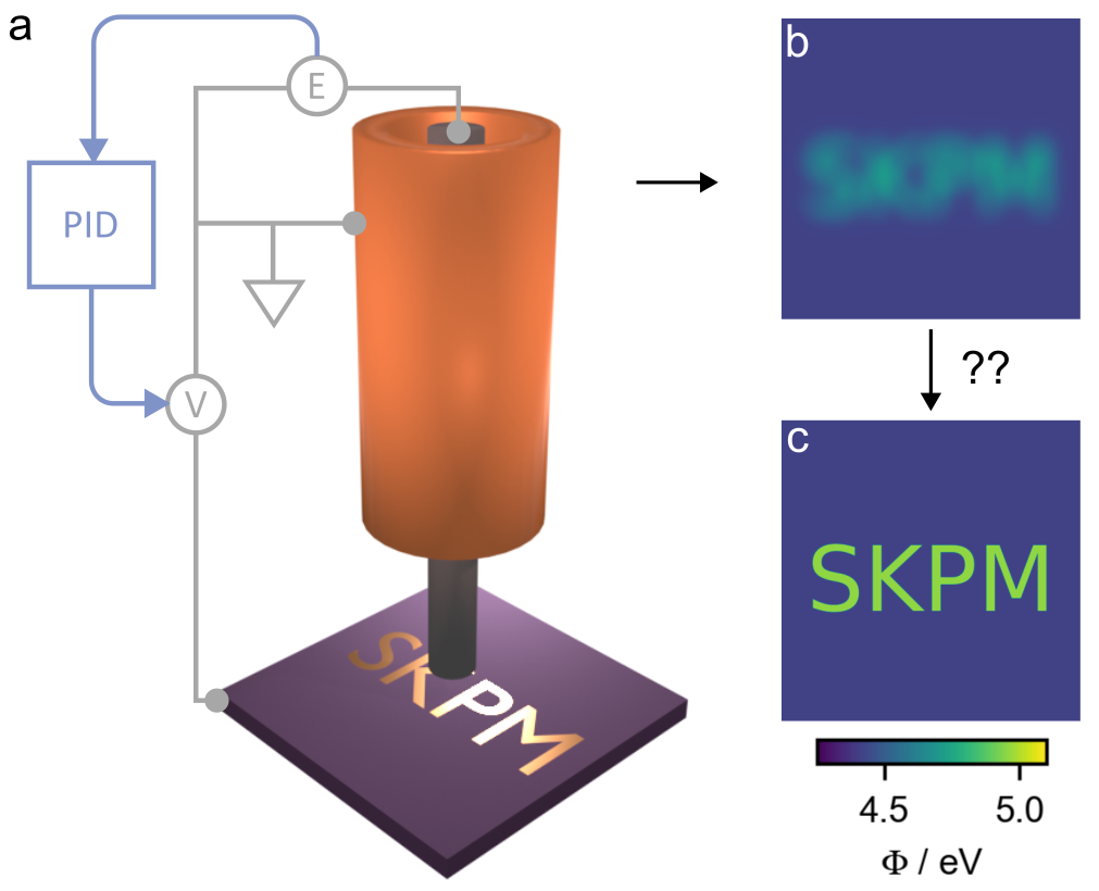
Figure 1: Principle of scanning Kelvin probe microscopy (SKPM). a SKPM entails scanning a conductive probe above a sample to estimate the local surface potential. The cylindrical metal probe is vibrated vertically, while a lock-in amplifier and PID use feedback adjust the backing potential, $V$, so that the current in the probe is minimised. b Voltage maps measured by SKPM are spatially distorted, due to the probe’s finite size, long-range electrostatics, and the temporal response of the electronics. c This paper is about extracting the true underlying surface potential from the measured signal, which we show is achievable by experimentally measuring the system’s PSF and using this to deconvolve raw measurements.

Toward addressing the problem, one can draw inspiration from optical microscopy. Like SKPM, optical images suffer from distortions, due to diffraction, optical imperfections, finite pixel sizes etc. To correct for these, a practical solution is to image the pattern created by a point-like emitter, e.g. a small fluorescent particle(Cole, Jinadasa, and Brown, 2011). When this target is significantly smaller than the system resolution, the image rendered is approximately the PSF.

Here, we show that the approach of experimentally measuring PSFs is not only viable, but effective and straightforwardly implemented in the case of SKPM. We restrict ourselves to the situation where the underlying signal is due to differences in material work functions on a planar surface, though in principle our ideas can be extended to other situations (e.g. variations in surface charge). We use common clean-room techniques to pattern regions with work function differences, which we image to extract PSFs. We find that when utilizing high scan speeds—which are necessary to probe large features—the measured PSFs can differ significantly from those that only account for the electrostatic interactions between the probe and sample. We show that this is due to incorporation of temporal information into the PSF—an issue that would be difficult to account for analytically/computationally, but that is solved relatively easily in experiment. Our results outline a practical and easily implemented approach toward getting quantitative information out of SKPM.

II Measurement Principal

II.1 Signal acquisition

Figure 1a depicts an SKPM probe positioned above a sample and the feedback system used to acquire an estimate for the spatially varying surface potential of interest, $V_{S}\equiv V_{S}(x)$. The probe vibrates vertically at a fixed amplitude and frequency, while a potential $V$ is applied to the electrode at or below the sample. The current drawn to the probe due to the vibration is measured by an electrometer ($E$) and further amplified by a lock-in amplifier which extracts the current signal due to the probe vibration and rejects noise at other frequencies. The signal acquired by SKPM is the value of the voltage, $V$, required to minimise the current induced in the probe as it is vibrated. This is accomplished by using feedback on the lock-in signal, e.g., sending it to proportional-integral-differential (PID) electronics and adjusting $V$ until the current amplitude is zero. In the naïve version of the analysis, the probe-sample system is assumed to form a capacitor, where the image charge drawn to the probe is given by

$$Q(t)=C(h(t))(V-V_{S}).$$ (1)

Here, $C(h)$ is the capacitance, and $h(t)$ is the time-varying height of the probe above the sample. By differentiating Eq. 1 with respect to time, setting equal to zero, and defining for $V_{m}\equiv V$ in this condition, we find

$$0=\frac{dQ}{dt}=\frac{dh}{dt}\frac{dC}{dh}(V_{m}-V_{S}).$$ (2)

Hence, for finite derivatives $dh/dt$ and $dC/dh$, we see that this condition is satisfied when

$$V_{m}(x)=V_{S}(x).$$ (3)

In other words, the simplest interpretation of raw SKPM data is that it is an exact, point-by-point copy of the surface potential of interest.

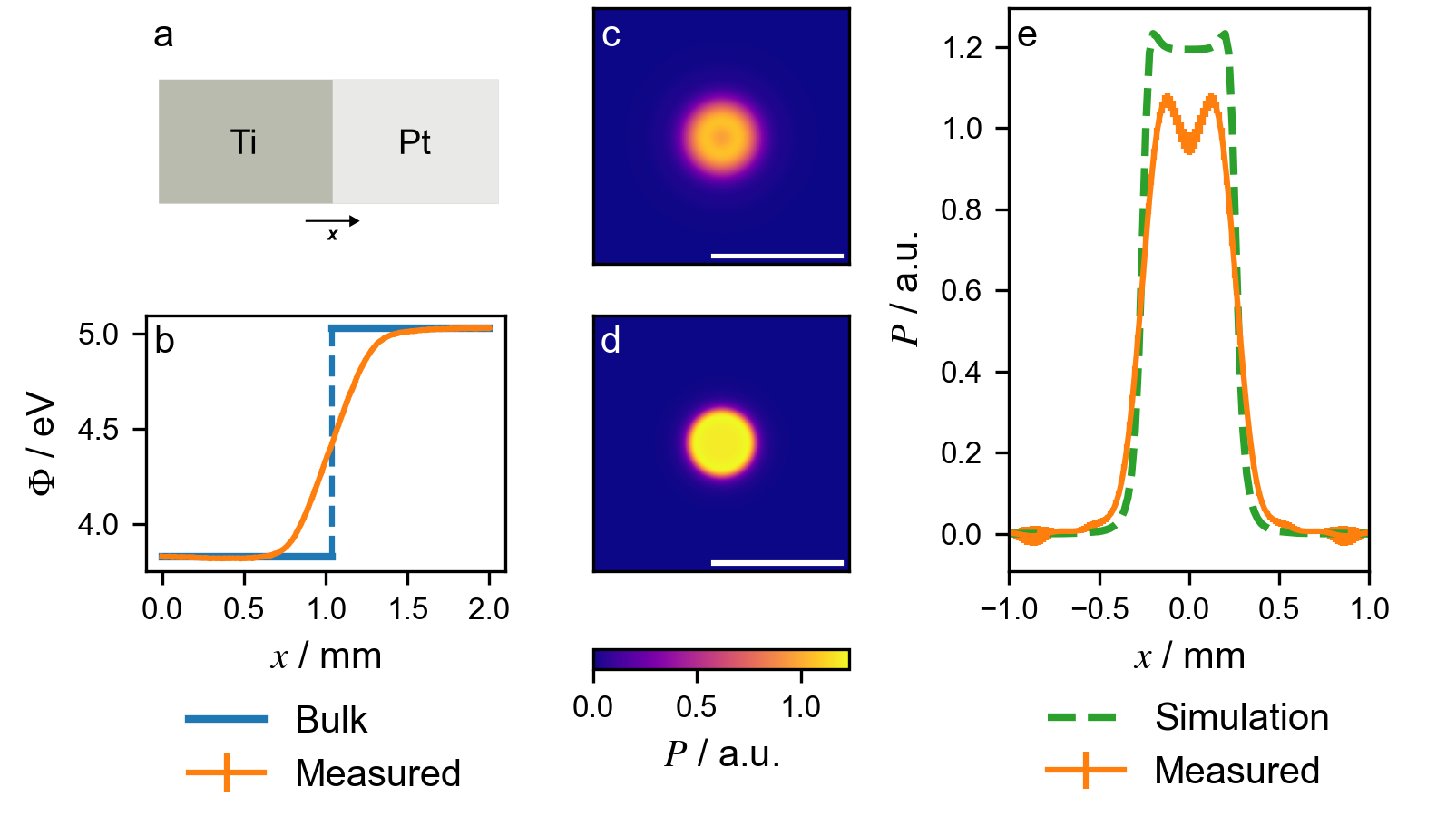
Figure 2: Comparison between a PSF estimated using an edge measurement and a simulated PSF. a Scanning an edge created at the boundary between two metals with distinct work functions produces b an estimate for the system edge spread function (ESF) along the scan direction. c Shows the system PSF estimated from the ESF measurement by assuming that the probe is rotationally symmetric. d,e Simulations produce a PSF with a similar width and qualitatively similar shape, but show non-negligible differences due to variations between the simulation geometry and the real probe. All scale bars correspond to 1 mm.

The above analysis doesn’t account for the finite size of the probe or long-range electrostatic interactions. These contributions can be incorporated by replacing the simple capacitance, $C(h)$, with an integral over a distributed capacitance, $\mathcal{C}(h,x)$ (Machleidt et al., 2009; Cohen et al., 2013). In this case, the SKPM condition becomes

$$0=\frac{d}{dh}\int_{S}(V_{m}(x)-V_{S}(\xi-x))\mathcal{C}(h,\xi)\ d\xi,$$ (4)

where $\xi$ is an integration variable. Solving this expression for $V_{m}$ gives

$$V_{m}(x)=\int_{S}P(x,\xi)V_{S}(\xi)\ d\xi$$ (5)

where we define the PSF, $P(x,\xi)$, which accounts for the terms involving the interaction of the probe at location $x$ with different sample positions $\xi$. Hence, a slightly more sophisticated analysis reveals that a raw SKPM measurement is the convolution of the underlying signal with a point spread function corresponding to the finite size of the probe and long-range interactions.

In practice, the situation is more complicated still, though for less obvious reasons. The measured signal depends not only on the electrostatic interactions between the probe and the sample, but also on the feedback system that measures the current and applies the voltage, $V$. Both the PID and lock-in amplifier require finite response times to produce stable signals. If the probe travels a significant distance over these timescales, then information from a range of locations is incorporated into the measurement. Additionally, faster scan speeds can introduce additional mechanical noise which will further distort the measured signal. Only for a stable system and when the probe is held at each location for long time relative to the response times of the PID/lock-in do we recover Eq. 5. Assuming these processes are linear, we can still write the measured voltage as a purely spatial convolution over a point spread function, but one that is velocity dependent; in other words,

$$V_{m}(x)=\int P(v\,|\,x,\xi)V_{S}(\xi)\ d\xi.$$ (6)

As the scan velocity approaches zero, $P(v\,|\,x,\xi)\rightarrow P(x,\xi)$, and the “fast scan” regime (Eq. 6) becomes equivalent to the “slow scan” regime (Eq. 5).

II.2 Signal deconvolution

In the previous section, we discussed the forward problem: given an underlying surface potential, $V_{S}(x)$, determine the resulting measurement, $V_{m}(x)$. However, what is usually required is the solution to the inverse problem: given the measurement, $V_{m}(x)$, determine the underlying signal, $V_{S}(x)$ (i.e., recover Fig. 1c from Fig. 1b). We start by writing the convolution over the PSF more compactly as

$$V_{m}=V_{S}\otimes P.$$ (7)

We would like to find an estimate for the true surface voltage map, $\bar{V}_{S}$. In the absence of measurement noise, and for a non-vanishing $P$, we can exactly recover the true surface voltage map, $V_{S}$, by

$$\bar{V}_{S}=V_{m}\otimes P^{-1}=(V_{S}\otimes P)\otimes P^{-1}=V_{S},$$ (8)

where $\otimes P^{-1}$ denotes the deconvolution with respect to $P$. This expression is relatively easy to calculate by taking advantage of the convolution theorem, i.e.

$$\bar{V}_{S}=\mathcal{F}^{-1}\left(\frac{\mathcal{F}(V_{m})}{\mathcal{F}(P)}\right),$$ (9)

where $\mathcal{F}$ and $\mathcal{F}^{-1}$ represent the Fourier transform and inverse Fourier transform, respectively.

Real systems suffer from measurement noise, which renders the equivalence of $\bar{V}_{S}$ and $V_{S}$ in Eq. 8 unattainable in practice. Mathematically, independent sources of noise, $N$, enter into the equation as $V_{m}=V_{S}\otimes P+N$, and contain high-frequency components which deconvolution can amplify. To reduce the effect of this, one approach is to simply apply a low-pass filter to $V_{m}$, which can be heuristically motivated given the finite size of probes(Pertl et al., 2022). However, in order to avoid discarding higher frequency information unnecessarily, an alternative is to use a weighted deconvolution, such as a Wiener filter(Machleidt et al., 2009; Cohen et al., 2013). Mathematically, this manifests itself as a modification to Eq. 9:

$$\bar{V}_{S}=\mathcal{F}^{-1}\left(\frac{\mathcal{F}(V_{m})}{\mathcal{F}(P)}\cdot\left(\frac{|\mathcal{F}(P)|^{2}}{|\mathcal{F}(P)|^{2}+\frac{1}{\textrm{SNR}(f)}}\right)\right),$$ (10)

where, $\textrm{SNR}(f)$ is the signal to noise ratio as a function of spatial frequency. The SNR can either be measured (e.g., by calculating the power spectral density of representative samples with known properties), or in certain circumstances assumed in conjunction with a frequency-relationship for the noise (e.g. Brownian noise $1/f^{2}$, pink noise $1/f$, etc.)

III Target Fabrication & Measurement

To experimentally determine the PSFs, we fabricate calibration targets using metals with different work functions. We work with two different types: an edge target, which produces a large signal but only provides information about the PSF in one direction(Claxton and Staunton, 2008; Zhang et al., 2012); and a disc target, which allows convenient measurement of the full 2-dimensional PSF from a single 2-dimensional scan. We utilise the edge target for measuring the slow scan PSF (Eq. 5) where we assume rotational symmetry of the PSF and are interested in a very accurate low noise estimate for the probe PSF. We use the disc target for estimating the fast scan PSF (Eq. 6) where the PSF is highly non-axisymmetric and our priority is on performing measurements in reasonable amounts of time under practical conditions.

We fabricate both targets using electron beam evaporation to deposit thin layers of different metals; full details are provided in the Supplemental Materials (SM). The edge target consists of a layer of platinum deposited on a titanium coated glass slide. The physical height of the platinum layer is small (12 nm) compared to the sample-tip separation (60 µm) so that its geometric influence can be ignored. These metals are chosen for their relatively large work function difference, which due to Fermi equalisation leads to a large contact potential difference and correspondingly large SKPM signal ($\sim$1 V). The disc target consists of a small, circular (400 $\mu$m diameter) gold disc deposited on a silicon wafer, creating a contact potential difference on the order of 0.5 eV. As with the edge target, the height of the gold-titanium disc is small (103 nm) compared to the scan height.

We perform SKPM measurements using a commercially available device (Biologic, M470). When SKPM is used for work function measurements, the signal ($\Delta\Phi$) is a relative measurement of the difference in work function between the probe and sample. As we explain in the SM, we convert relative work function differences to absolute work function values by first measuring the SKPM voltage using a reference sample of highly ordered pyrolytic graphite (HOPG). The work function is then given by $\Phi=\Delta\Phi+\Delta\Phi_{\textrm{HOPG}}$, where $\Delta\Phi_{\textrm{HOPG}}$ is the difference between the literature value for the HOPG work function and the measured value. To estimate the SNR for deconvolution (i.e., Eq. 10), we look at the power spectral density of a relatively flat region and use this to estimate a power-law relationship between SNR and frequency.

To demonstrate the effect of acquisition parameters and the temporal dependence of acquired measurements, we perform slow scans with step-mode acquisition and fast scans with sweep-mode acquisition. The step-mode acquisition entails moving the probe between specific points and holding it fixed until the SKPM signal has stabilised (i.e., until we can ignore effects from the movement and settling time of the PID/lock-in amplifier). Sweep-mode acquisition involves moving the probe continuously across the sample at a constant velocity, resulting in a temporally distorted signal depending on the scan speed and feedback parameters.

IV Results & Discussion

IV.1 Experimentally determining PSFs in the quasi-static limit

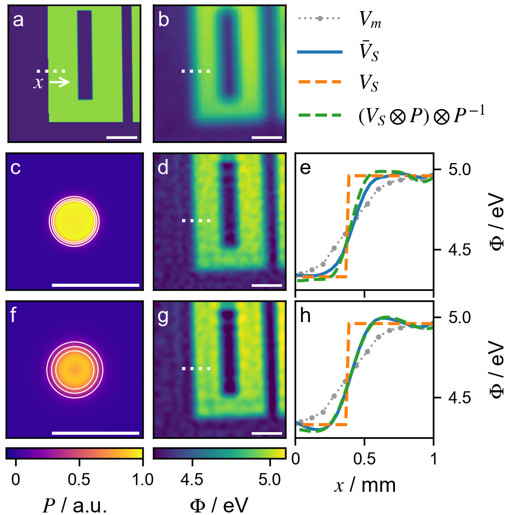
Figure 3: Comparison between deconvolution with different PSFs in slow scans. a Scanning a gold-on-silicon target ($V_{S}$) with sharp features produces b a measured ($V_{m}$) signal with low contrast and blurred-out features. c–e Deconvolution with c the simulated PSF from Fig. 2d produces d an image with higher contrast; however, as shown in e, a slice through the deconvolved image ($\bar{V}_{S}$) differs from the ideal scenario ($(V_{S}\otimes P)\otimes P^{-1}$). f–h The experimentally measured probe PSF produces a improved estimate for the original signal. Scale bars show 1 mm.

We now demonstrate how a PSF can be determined experimentally. We start in the slow scan regime, i.e. at speeds that are small enough such that Eq. 5 applies. The main difficulty in measuring the slow scan PSF is signal strength compared to measurement noise. Signal strength can be improved by increasing the work function difference between the target and surface or increasing the size of the target, while noise can be reduced with repeated measurements and reduced scan speed. We have found that a good solution for the slow-scan regime is to perform a 1-dimensional scan over a sharp edge between two materials with distinct work functions (Figure 2a). Even so, extremely slow speeds are required for probe motion to be completely negligible. We utilize a step size of 5 µm, moving at 5 µm/s between points and dwelling at each point for 3.5 s. To improve SNR, we repeat and average multiple lines. In this process, a single line scan takes approximately 45 minutes, and the ensemble takes more than seven hours. The final result is shown in Fig. 2b.

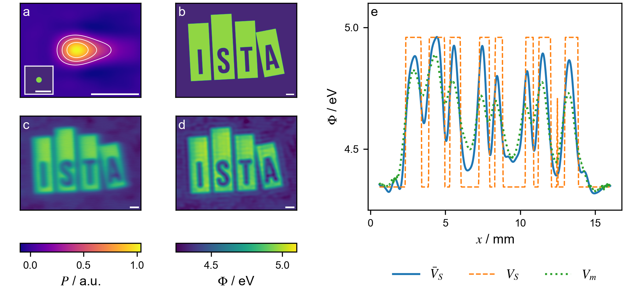
Figure 4: PSF and deconvolution for a fast scan. a Fast scans produce a significantly broadened and asymmetric PSF ($P$), particularly along the scan direction. b,c When the same parameters are used to scan a large target ($V_{S}$, b), this produces a blurred-out image ($V_{m}$, c). d Deconvolution of the measured signal with the PSF produces a significantly improved estimate for the underlying signal ($\bar{V}_{S}$). e A slice shows quantitatively how the contrast is improved by the deconvolution. Scale bars correspond to 1 mm.

To obtain the PSF, we first calculate the line spread function from the derivative of the line scan, and then in Fourier space we interpolate the 1-dimensional transform of the line spread function to a 2-dimensional map assuming rotational symmetry. Taking the inverse transform we get an approximation of the real space PSF (see SM for full details). The result is shown in (Fig. 2c). The cross section of this PSF (Fig. 2e) has a non-intuitive feature: a ring of higher intensity towards the edge of the probe. To investigate this further and perform a sanity-check of our strategy, we perform numerical simulations for a second, independent estimate of the PSF (Fig. 2d,e; see SM for details on simulations). The simulations produce a decent estimate for the PSF, but the differences are non-negligible. The simulated PSF has a higher amplitude, is slightly narrower, and exhibits a more subdued ring at the edge. We suspect these differences are due to physical features of the probe that the idealised simulation geometry cannot capture. For example, visual inspection of the probe reveals it is not perfectly cylindrical, and high-speed video reveals subtle horizontal vibrations in addition to the vertical motion (see SM). This speculation is supported qualitatively by the fact that in our simulations, we observe that even small changes to the probe shape (e.g. rounding edges) can have a significant effect on the PSF (see SM). The inability of simulations to faithfully reproduce the experiments even in the slow-scan regime highlight the need for measuring PSFs.

With a PSF in hand, we turn our attention to reconstructing an underlying signal source from an actual measurement. Fig. 3a illustrates our gold-on-silicon target, where the pattern consists a series of vertical/horizontal stripes switching between the two materials. We scan over this target at a slightly lower resolution (80 $\mu$m steps) and slightly larger speed (20 $\mu$m/s with 0.6 s dwell time) so that the scan doesn’t take unreasonably long. This produces the measured voltage map, $V_{m}$, of Fig. 3b. Using Eq. 10 and the simulated and measured probe PSFs of Fig. 2, we find that we can indeed recover estimates with improved resolution/contrast (Fig. 3c–h). We show in the SM that these recoveries already suffer from slightly elevated scan speed; trying to eliminate temporal information in the PSF entails compromises between speed and resolution that are difficult to balance. As we show in the next section, the better solution is to simply incorporate the probe motion into the PSF.

IV.2 Determining PSFs for rapid measurements

Without compromising scan speed, we would like to be able to characterise large patterns of interest with high spatial resolution. As mentioned previously, when the distortions introduced by fast scanning are linear, then one can anticipate a velocity-dependent PSF, $P(\,v\,|x,\xi)$, that nonetheless connects the measured signal, $V_{m}$, to the underlying signal, $V_{S}$, via spatial convolution, as in Eq. 6. In order to acquire this PSF, we straightforwardly perform a scan with the same measurement parameters as we use for the sample measurement. While we could repeat the procedure involving the edge PSF described above, we now no longer have to worry about scanning slowly to stay in a regime where Eq. 5 is applicable. Moreover, scanning fast creates an additional source of broadening to the PSF, making the use of larger targets more practical. Figure 4 shows how we put this into practice. To get a velocity-dependent scan, we now operate the SKPM in sweep (continuous) mode (as opposed to step mode), and with a significantly higher speed of 200 µm/s. The size of the disk renders a large PSF signal, helping to ameliorate the noise issues mentioned previously. As is visually apparent in the image of the PSF itself (Fig. 4a), the velocity dependence blurs the image in the scan direction (left to right).

Next, we scan a large and detailed target ($\sim$1.5$\times$1.0 cm²), as shown in Fig. 4b, which again consists of gold patterned onto a silicon wafer. The scan parameters are intentionally set to be the same as in the PSF of Fig. 4a. The resulting raw voltage map is shown in Fig. 4c. Comparing this to the slower scans of Fig. 2, the spatial blurring is much more apparent. Moreover, it is evident that this has the same left-to-right tail as the corresponding PSF. However, upon spatially deconvolving this scan with the corresponding PSF, the blur is reduced (Fig. 4d). We validate this quantitatively in Fig. 4e, where we plot the target, raw, and recovered values on top of each other, illustrating that the recovered voltages are much sharper and lie much closer to the target values.

V Conclusion

In this work we demonstrate how the PSFs relevant to scanning Kelvin probe microscopy (SKPM) can be experimentally determined. We find that measured PSFs can differ significantly from those estimated using simulations, especially for rapid scans where the finite response of the feedback system and additional noise further broaden the PSFs. We demonstrate that a practical approach for accounting for the effect of noise in a scan is to measure the PSF using similar scan parameters to those used during measurement acquisition. We utilize two methods for estimating PSFs: one using a edge target, which provides good signal strength but only gives information about the PSF in one direction; and the second using a disc, which provides information about the full 2-dimensional PSF from a single 2-dimensional scan. While both methods could be used to acquire PSFs, we found that the disc was particularly useful for faster scans, where the PSFs tend to be non-axissymetric. The edge method is more suited to acquiring lower noise PSFs but requires assumptions about the PSF symmetry or multiple measurements with different edge angles to estimate the 2-dimensional PSF.

While the larger probes used in SKPM allow direct measurement of the PSF, for smaller probes the required spot size and the corresponding decrease in the signal to noise ratio makes experimental measurement of such PSFs difficult. We explore targets involving work function differences between metals, however other approaches such as depositing charge spots or creating a artificial potential step(Brouillard et al., 2022) could further improve the signal to noise ratio. Although we focused on SKPM, this procedure could also be useful for characterising and correcting for temporal effects in related methods (Checa et al., 2023). Additional modelling of the signal acquisition pipeline could also be useful for determining the effective measurement PSFs from simulated PSFs, this could be particularly relevant for smaller probes such as the nano-scale probes used in KPFM. The results presented here could be useful for scanning larger samples, particularly with larger probes at faster scanning speeds while achieving decent resolution in the reconstructed images.

Author Declarations

Conflict of Interest

The authors have no conflicts to disclose.

CRediT Author Statement

IL: Conceptualization; Formal analysis; Simulation; Investigation; Writing – Original Draft. FP: Investigation; Resources. LS: Resources. SW: Writing – Review & Editing; Supervision; Funding acquisition.

Data Availability Statement

The data that support the findings of this study are available from the corresponding author upon reasonable request.

References

References

- Zisman (1932) W. A. Zisman, “A new method of measuring contact potential differences in metals,” Rev. Sci. Instrum. 3, 367–370 (1932).
- Craig and Radeka (1970) P. P. Craig and V. Radeka, “Stress Dependence of Contact Potential: The ac Kelvin Method,” Rev. Sci. Instrum. 41, 258–264 (1970).
- Nazarov and Thierry (2019) A. Nazarov and D. Thierry, “Application of Scanning Kelvin Probe in the Study of Protective Paints,” Front. Mater. 6, 462587 (2019).
- Nazarov, Olivier, and Thierry (2012) A. Nazarov, M.-G. Olivier, and D. Thierry, “SKP and FT-IR microscopy study of the paint corrosion de-adhesion from the surface of galvanized steel,” Progress in Organic Coatings 74, 356–364 (2012), application of Electrochemical Techniques to Organic Coatings.
- Baytekin et al. (2011) H. T. Baytekin, A. Z. Patashinski, M. Branicki, B. Baytekin, S. Soh, and B. A. Grzybowski, “The Mosaic of Surface Charge in Contact Electrification,” Science 333, 308–312 (2011).
- Bai et al. (2021) X. Bai, A. Riet, S. Xu, D. J. Lacks, and H. Wang, “Experimental and Simulation Investigation of the Nanoscale Charge Diffusion Process on a Dielectric Surface: Effects of Relative Humidity,” J. Phys. Chem. C 125, 11677–11686 (2021).
- Hackl, Schitter, and Mesquida (2022) T. Hackl, G. Schitter, and P. Mesquida, “AC Kelvin Probe Force Microscopy Enables Charge Mapping in Water,” ACS Nano 16, 17982–17990 (2022).
- Ørjan G. Martinsen and Heiskanen (2023) Ørjan G. Martinsen and A. Heiskanen, “Chapter 7 - electrodes,” in Bioimpedance and Bioelectricity Basics (Fourth Edition), edited by Ørjan G. Martinsen and A. Heiskanen (Academic Press, Oxford, 2023) fourth edition ed., pp. 175–248.
- Nonnenmacher, O’Boyle, and Wickramasinghe (1991) M. Nonnenmacher, M. P. O’Boyle, and H. K. Wickramasinghe, “Kelvin probe force microscopy,” Appl. Phys. Lett. 58, 2921–2923 (1991).
- Glatzel, Gysin, and Meyer (2022) T. Glatzel, U. Gysin, and E. Meyer, “Kelvin probe force microscopy for material characterization,” Microscopy 71, i165–i173 (2022).
- Melitz et al. (2011) W. Melitz, J. Shen, A. C. Kummel, and S. Lee, “Kelvin probe force microscopy and its application,” Surf. Sci. Rep. 66, 1–27 (2011).
- Cohen et al. (2013) G. Cohen, E. Halpern, S. U. Nanayakkara, J. M. Luther, C. Held, R. Bennewitz, A. Boag, and Y. Rosenwaks, “Reconstruction of surface potential from Kelvin probe force microscopy images,” Nanotechnology 24, 295702 (2013).
- Machleidt et al. (2009) T. Machleidt, E. Sparrer, D. Kapusi, and K.-H. Franke, “Deconvolution of Kelvin probe force microscopy measurements—methodology and application,” Meas. Sci. Technol. 20, 084017 (2009).
- Ren et al. (2023) B. Ren, L. Chen, R. Chen, R. Ji, and Y. Wang, “Noise Reduction of Atomic Force Microscopy Measurement Data for Fitting Verification of Chemical Mechanical Planarization Model,” Electronics 12, 2422 (2023).
- Checa et al. (2023) M. Checa, A. S. Fuhr, C. Sun, R. Vasudevan, M. Ziatdinov, I. Ivanov, S. J. Yun, K. Xiao, A. Sehirlioglu, Y. Kim, P. Sharma, K. P. Kelley, N. Domingo, S. Jesse, and L. Collins, “High-speed mapping of surface charge dynamics using sparse scanning Kelvin probe force microscopy,” Nat. Commun. 14, 1–12 (2023).
- Ziegler et al. (2013) D. Ziegler, T. R. Meyer, R. Farnham, C. Brune, A. L. Bertozzi, and P. D. Ashby, “Improved accuracy and speed in scanning probe microscopy by image reconstruction from non-gridded position sensor data,” Nanotechnology 24, 335703 (2013).
- Cole, Jinadasa, and Brown (2011) R. W. Cole, T. Jinadasa, and C. M. Brown, “Measuring and interpreting point spread functions to determine confocal microscope resolution and ensure quality control,” Nat. Protoc. 6, 1929–1941 (2011).
- Pertl et al. (2022) F. Pertl, J. C. Sobarzo, L. Shafeek, T. Cramer, and S. Waitukaitis, “Quantifying nanoscale charge density features of contact-charged surfaces with an FEM/KPFM-hybrid approach,” Phys. Rev. Mater. 6, 125605 (2022).
- Claxton and Staunton (2008) C. D. Claxton and R. C. Staunton, “Measurement of the point-spread function of a noisy imaging system,” J. Opt. Soc. Am. A, JOSAA 25, 159–170 (2008).
- Zhang et al. (2012) X. Zhang, T. Kashti, D. Kella, T. Frank, D. Shaked, R. Ulichney, M. Fischer, and J. P. Allebach, “Measuring the modulation transfer function of image capture devices: what do the numbers really mean?” in Proceedings Volume 8293, Image Quality and System Performance IX, Vol. 8293 (SPIE, 2012) pp. 64–74.
- Brouillard et al. (2022) M. Brouillard, N. Bercu, U. Zschieschang, O. Simonetti, R. Mittapalli, H. Klauk, and L. Giraudet, “Experimental determination of the lateral resolution of surface electric potential measurements by Kelvin probe force microscopy using biased electrodes separated by a nanoscale gap and application to thin-film transistors,” Nanoscale Adv. 4, 2018–2028 (2022).
- Zerweck et al. (2005) U. Zerweck, C. Loppacher, T. Otto, S. Grafström, and L. M. Eng, “Accuracy and resolution limits of Kelvin probe force microscopy,” Phys. Rev. B 71, 125424 (2005).
- Glatzel et al. (2007) Th. Glatzel, M. Ch. Lux-Steiner, E. Strassburg, A. Boag, and Y. Rosenwaks, “Principles of Kelvin Probe Force Microscopy,” in Scanning Probe Microscopy (Springer, New York, NY, New York, NY, USA, 2007) pp. 113–131.
- Salerno and Dante (2018) M. Salerno and S. Dante, “Scanning Kelvin Probe Microscopy: Challenges and Perspectives towards Increased Application on Biomaterials and Biological Samples,” Materials 11 (2018), 10.3390/ma11060951.
- Hoffman and Leibowitz (1972) D. Hoffman and D. Leibowitz, “Effect of Substrate Potential on Al2O3 Films Prepared by Electron Beam Evaporation,” J. Vac. Sci. Technol. 9, 326–329 (1972).
- Volmer et al. (2021) F. Volmer, I. Seidler, T. Bisswanger, J.-S. Tu, L. R. Schreiber, C. Stampfer, and B. Beschoten, “How to solve problems in micro- and nanofabrication caused by the emission of electrons and charged metal atoms during e-beam evaporation,” J. Phys. D: Appl. Phys. 54, 225304 (2021).
- Turetta et al. (2021) N. Turetta, F. Sedona, A. Liscio, M. Sambi, and P. Samorì, “Au(111) Surface Contamination in Ambient Conditions: Unravelling the Dynamics of the Work Function in Air,” Adv. Mater. Interfaces 8, 2100068 (2021).
- Yu, Lee, and Jeong (2023) Y. Yu, D. Lee, and B. Jeong, “The dependence of the work function of Pt(111) on surface carbon investigated with near ambient pressure X-ray photoelectron spectroscopy,” Appl. Surf. Sci. 607, 155005 (2023).
- Bai et al. (2023) R. Bai, N. L. Tolman, Z. Peng, and H. Liu, “Influence of Atmospheric Contaminants on the Work Function of Graphite,” Langmuir 39, 12159–12165 (2023).
- Sugimura et al. (2002) H. Sugimura, Y. Ishida, K. Hayashi, O. Takai, and N. Nakagiri, “Potential shielding by the surface water layer in Kelvin probe force microscopy,” Appl. Phys. Lett. 80, 1459–1461 (2002).