$\bm{\bar{b}\bar{b}ud}$ and $\bm{\bar{b}\bar{b}us}$ tetraquarks from lattice QCD using symmetric correlation matrices with both local and scattering interpolating operators

Abstract

We study the $\bar{b}\bar{b}ud$ tetraquark with quantum numbers $I(J^{P})=0(1^{+})$ as well as the $\bar{b}\bar{b}us$ tetraquark with quantum numbers $J^{P}=1^{+}$ using lattice QCD. We improve on existing work by including both local and scattering interpolating operators on both sides of the correlation functions and use symmetric correlation matrices. This allows not only a reliable determination of the energies of QCD-stable tetraquark ground states, but also of low-lying excited states, which are meson-meson scattering states. The latter is particularly important for future finite-volume scattering analyses. Here, we perform chiral and continuum extrapolations of just the ground-state energies, for which finite-volume effects are expected to be small. Our resulting tetraquark binding energies, $-100\pm 10\>^{+36}_{-43}\>\>{\rm MeV}$ for $\bar{b}\bar{b}ud$ and $-30\pm 3\>^{+11}_{-31}\>\>{\rm MeV}$ for $\bar{b}\bar{b}us$, are consistent with other recent lattice-QCD predictions.

I Introduction

Mesons, which are hadrons with integer spin, are typically composed of one valence quark and one valence antiquark. However, they can as well contain two valence quarks and two valence antiquarks. Such exotic states are called tetraquarks. In this work we use lattice QCD to study two particular antiheavy-antiheavy-light-light four-quark systems, the $\bar{b}\bar{b}ud$ tetraquark with quantum numbers $I(J^{P})=0(1^{+})$ and the $\bar{b}\bar{b}us$ tetraquark with quantum numbers $J^{P}=1^{+}$. These tetraquarks are expected to be QCD-stable (i.e., have a mass lower than the sum of the masses of the lightest possible strong-decay products, a pseudoscalar and a vector heavy-light meson in this case) for sufficiently large heavy-quark mass [1, 2, 3]. Accurately predicting the binding energies at the physical $b$-quark mass is quite challenging. Approaches using potential models, effective field theories, and QCD sum rules [1, 2, 4, 5, 6, 7, 8, 9, 10, 11, 12, 13, 3, 14, 15, 16, 17, 18, 19, 20, 21, 22, 23, 24, 25, 26, 27, 28, 29, 30, 31, 32] gave a wide spread of results for the binding energy of the $\bar{b}\bar{b}ud$ system, and did not all predict the $\bar{b}\bar{b}us$ mass to be below threshold (see, e.g., the summary plots in Fig. 13 in the conclusions section of this paper). On the other hand, studies using lattice QCD consistently find both the $\bar{b}\bar{b}ud$ and $\bar{b}\bar{b}us$ tetraquarks to be QCD-stable. While early investigations based on static potentials from lattice QCD and the Born-Oppenheimer approximation slightly underestimated the binding energy of the $\bar{b}\bar{b}ud$ tetraquark [33, 34, 35, 36, 37], more recent rigorous full lattice-QCD simulations [38, 39, 40, 41, 42, 43, 44] obtained binding energies of $\mathcal{O}(100\,\text{MeV})$ for the $\bar{b}\bar{b}ud$ tetraquark with $I(J^{P})=0(1^{+})$ and $\mathcal{O}(50\,\text{MeV})$ for the $\bar{b}\bar{b}us$ tetraquark with $J^{P}=1^{+}$, with good agreement within statistical and systematic uncertainties among the more advanced calculations.

There are further antiheavy-antiheavy-light-light systems that are promising with respect to the existence of tetraquark bound states or resonances, but for whom the situation is less clear. Two such candidates are the $\bar{b}\bar{c}ud$ systems with quantum numbers $I(J^{P})=0(0^{+})$ and $I(J^{P})=0(1^{+})$. Independent groups carrying out full lattice-QCD simulations have arrived at different conclusions. The existence of a strong-interaction-stable $\bar{b}\bar{c}ud$ tetraquark with $I(J^{P})=0(1^{+})$ was initially reported in Ref. [45] but later revoked in Ref. [46]. In Ref. [42], we did not find evidence for QCD-stable $\bar{b}\bar{c}ud$ bound states, but could not rule out shallow bound states. Other authors found an indication for a $\bar{b}\bar{c}ud$ bound state with $I(J^{P})=0(1^{+})$ below threshold [47, 48]. The conclusions of these studies were based only on the finite-volume ground-state energy. In a recent project carried out in parallel to this work we revisited both $\bar{b}\bar{c}ud$ systems taking into account also finite-volume energies of low-lying excitations. We found strong indication for very shallow bound states [49].

Another interesting system is $\bar{b}\bar{b}ud$ with quantum numbers $I(J^{P})=0(1^{-})$. This system has not yet been investigated in full lattice QCD, but has been explored in the Born-Oppenheimer approximation using lattice-QCD static potentials. While, at first, a tetraquark resonance was predicted in a crude way (completely neglecting effects of the heavy-quark spins) [50], a refined study that is still ongoing suggests that neither a bound state nor a resonance exist in the region near the $BB$ threshold [51]. Given that the Born-Oppenheimer approximation with lattice-QCD static potentials seems to underestimate the binding energy of QCD-stable antiheavy-antiheavy-light-light systems, the existence of a $I(J^{P})=0(1^{-})$, $\bar{b}\bar{b}ud$ resonance is not yet excluded and should be investigated in full lattice QCD.

To rigorously search for tetraquark resonances or shallow bound states in full lattice QCD, determinations of the meson-meson scattering amplitudes both below and above the relevant thresholds are mandatory. Such computations are typically based on Lüscher’s method [52] and its generalizations (see the review in Ref. [53]), and require a precise computation of all relevant low-lying finite-volume energy levels. To be able to resolve all of these energy levels, one needs a sufficiently large basis of interpolating operators that must be able to capture the spatial structures of all relevant states. This requires the use of both local operators, in which the four quarks are placed at or near the same spatial point and jointly projected to the desired total momentum, and scattering operators, which are constructed from products of two individually momentum-projected meson operators.

Previous full lattice-QCD studies of antiheavy-antiheavy-light-light systems containing anti-bottom quarks used either exclusively local operators [38, 39, 40, 41, 43, 44, 48] or a combination of local and scattering operators with the latter employed only at the sink of the correlation functions [40, 42]. In this paper (and in our very recent work [49] on the $\bar{b}\bar{c}ud$ system, which we carried out in parallel) we implemented and used, for the first time in the bottom sector, local and scattering interpolating operators both at the source and at the sink of correlation functions, leading to symmetric correlation matrices containing both types of operators. Here we focus again on the $\bar{b}\bar{b}ud$ system with quantum numbers $I(J^{P})=0(1^{+})$ and the $\bar{b}\bar{b}us$ system with quantum numbers $J^{P}=1^{+}$. We demonstrate that we are able to extract the energy levels of several meson-meson scattering states in addition to the ground-state energy below the lowest meson-meson threshold (however, in contrast to Ref. [49], here we only included scattering operators with vanishing relative momenta and were therefore only able to resolve the subset of scattering states of that type).

We use a lattice setup quite different from our previous lattice-QCD studies [40, 42] of antiheavy-antiheavy-light-light systems. The reason is that in our previous work we could reuse existing domain-wall point-to-all propagators previously generated for other projects [54, 55, 56, 57]. However, the computation of symmetric correlation matrices with both local and scattering operators is not possible with only point-to-all propagators. One additionally needs stochastic timeslice-to-all propagators for the correlation matrix elements with scattering operators at the source. Technical details can be found, for example, in Ref. [58], which includes a discussion of the one-end-trick that is essential for computing matrix elements with stochastic propagators. Since we had to recompute light and strange quark propagators, we decided to use a computationally cheaper mixed-action setup previously employed by the PNDME collaboration [59, 60]: clover-improved Wilson (with HYP link smearing) valence $u$, $d$, and $s$ quarks on the $(2+1+1)$-flavor gauge-link ensembles generated by the MILC collaboration using the highly improved staggered quark (HISQ) action [61]. As before, we use lattice NRQCD for the heavy $\bar{b}$ quarks.

While it is certainly interesting to revisit the $\bar{b}\bar{b}ud$ system with quantum numbers $I(J^{P})=0(1^{+})$ and the $\bar{b}\bar{b}us$ system with quantum numbers $J^{P}=1^{+}$, now for the first time with a combination of local and scattering operators and symmetric correlation matrices, the main motivation of this work is rather to explore and prepare computational methods suited to study antiheavy-antiheavy-light-light tetraquark resonances. As discussed above, this requires a precise determination of energy levels of low-lying scattering states. We demonstrate that this works well with our setup, and also present evidence that it is not feasible without scattering operators.

This article is organized in the following way. In Section II we briefly summarize our lattice setup. In Section III we discuss the interpolating operators for the two systems we investigate and the corresponding correlation functions. In Section IV we provide our lattice results for the energies of the pseudoscalar and vector $B$ and $B_{s}$ mesons and determine their kinetic masses from the momentum dependence of these energies. In Section V we present the numerical results for the low-lying finite-volume energy levels of the $\bar{b}\bar{b}ud$ and $\bar{b}\bar{b}us$ four-quark systems. We also explore the importance of each of our interpolating operators, which provides certain insights concerning the structure of the low-lying states. In Section VI we comment on finite-volume effects and the left-hand cut issue. Our extrapolations of the binding energies to the physical pion mass and continuum limit are discussed in Section VII. Finally, we summarize the main points of our work in Section VIII and give a brief outlook. Note that results obtained at an early stage of this project were presented at the Lattice 2022 conference [62].

II Lattice setup

We use $(2+1+1)$-flavor gauge-link ensembles generated by the MILC collaboration using the highly improved staggered quark (HISQ) action and a one-loop Symanzik improved gauge action (see Ref. [61] for details). The main properties of the seven ensembles, which differ in the lattice spacing, the spatial volume, and the pion mass, are collected in Table 1. The relative lattice spacings were determined using $r_{1}/a$, which is related to the static quark-antiquark force $F(r)$ and defined via $r_{1}^{2}F(r_{1})=1$; the physical value $r_{1}=0.3106(8)(14)(4)\,\text{fm}$ was obtained through an analysis of pseudoscalar decay constants [61, 63]. We note that the ensembles a12m220S, a12m220 and a12m220L have the same gauge coupling and bare light quark mass and only differ in the number of lattice sites in the spatial directions. Thus, they are particularly suited to investigate the volume dependence of energy eigenvalues.

ensemble	$N_{s}^{3}\times N_{t}$	$a$ [fm]	$m_{\pi}^{(\textrm{sea})}$ [MeV]	$m_{\pi}^{(\text{val})}$ [MeV]	$N_{\text{conf}}$
a15m310	$16^{3}\times 48$	0.1510(20)	$306.9(5)$	$320.6(4.3)$	$11554$
a12m310	$24^{3}\times 64$	0.1207(11)	$305.3(4)$	$310.2(2.8)$	$\phantom{0}1053$
a12m220S	$24^{3}\times 64$	0.1202(12)	$218.1(4)$	$225.0(2.3)$	$\phantom{0}1020$
a12m220	$32^{3}\times 64$	0.1184(10)	$216.9(2)$	$227.9(1.9)$	$\phantom{0}1000$
a12m220L	$40^{3}\times 64$	0.1189(09)	$217.0(2)$	$227.6(1.7)$	$\phantom{0}1030$
a09m310	$32^{3}\times 96$	0.0888(08)	$312.7(6)$	$313.0(2.8)$	$\phantom{0}1166$
a09m220	$48^{3}\times 96$	0.0872(07)	$220.3(2)$	$225.9(1.8)$	$\phantom{00}657$

Table 1: Gauge-link ensembles used in this work. Here, $N_{s}$, $N_{t}$ are the numbers of lattice sites in spatial and temporal directions, $a$ is lattice spacing, $m_{\pi}^{(\rm sea)}$ is the HISQ sea-quark pion mass (taste $\gamma_{5}$), and $N_{\text{conf}}$ is the number of gauge-link configurations [61]. Also shown are the results for the valence pion masses $m_{\pi}^{(\rm val)}$ computed on these ensembles using the Wilson-clover action with the parameters in Table 2 [59, 60].

For the valence $u$, $d$, and $s$ quarks, we use the Wilson-clover action with HYP-smeared gauge links to suppress exceptional configurations that can appear in a mixed-action setup (see the detailed discussion in Section II.A in Ref. [59]). This mixed-action setup was tested and successfully used by the PNDME collaboration in the context of computations of isovector and isoscalar tensor charges of the nucleon [59, 60]. We use the values for the bare quark masses and the Sheikholeslami-Wohlert coefficient tuned and provided by the PNDME collaboration (see Table 2 as well as Table II of Ref. [59] and Table I and Table II of Ref. [60]). The corresponding valence-quark pion masses are listed in Table 1 and quite similar to their counterparts computed within the unitary setup. A similar statement holds for the kaon masses, where the $s$-quark mass is close to the physical $s$-quark mass for all seven ensembles.

ensemble		$am_{l}^{(\text{val})}$		$am_{s}^{(\text{val})}$		$c_{\textrm{sw}}$		$am_{b}$		$u_{0L}$		$c_{1}$	$c_{5}$	$c_{6}$
a15m310		$-0.0893\phantom{0}$		$-0.021\phantom{0}\phantom{0}\phantom{0}$		$1.05945$		$3.42$		$0.8195$		$1.36$	$1.21$	$1.36$
a12m310		$-0.0695\phantom{0}$		$-0.018718$		$1.05094$		$2.66$		$0.834\phantom{0}$		$1.31$	$1.16$	$1.31$
a12m220S, a12m220, a12m220L		$-0.075\phantom{0}\phantom{0}$		$-0.02118\phantom{0}$		$1.05091$		$2.62$		$0.8349$		$1.31$	$1.16$	$1.31$
a09m310		$-0.05138$		$-0.016075$		$1.04243$		$1.91$		$0.8525$		$1.21$	$1.12$	$1.21$
a09m220		$-0.0554\phantom{0}$		$-0.01761\phantom{0}$		$1.04239$		$1.90$		$0.8521$		$1.21$	$1.12$	$1.21$

Table 2: Parameters of the Wilson-clover and NRQCD valence-quark actions. Here, $am_{l}^{(\text{val})}$ and $am_{s}^{(\text{val})}$ are the bare light and strange quark masses and $c_{\textrm{sw}}$ is the Sheikholeslami-Wohlert coefficient [59, 60]. In the NRQCD action, $am_{b}$ is the bare $b$-quark mass, $u_{0L}$ is the Landau-gauge mean link used for tadpole improvement, and $c_{1}$, $c_{5}$, $c_{6}$ are matching coefficients of kinetic terms (see Ref. [64] for details).

The $b$ quarks appear only as valence quarks and are implemented using lattice NRQCD [65]. We use the same order-$v^{4}$ action as in Ref. [64]. In contrast to the light and strange valence-quark action, the gauge links in the NRQCD action are not smeared. The matching coefficients of the kinetic terms, $c_{1}$, $c_{5}$, and $c_{6}$, include one-loop radiative corrections, while the other matching coefficients are set to their tree-level values. All parameters were taken from Tables II and III in Ref. [64] and are also reproduced here in Table 2.

III Interpolating operators and correlation functions

III.1 $\bar{b}\bar{b}ud$ and $\bar{b}\bar{b}us$ four-quark systems

III.1.1 Interpolating operators for $\bar{b}\bar{b}ud$ with $I(J^{P})=0(1^{+})$

For the $\bar{b}\bar{b}ud$ case, we use exactly the same interpolating operators as in our previous work [40] (but now compute all $5\times 5$ correlation matrix elements): three local operators

$$\mathcal{O}_{1}=\mathcal{O}_{[BB^{\ast}](0)}=\frac{1}{\sqrt{V_{s}}}\sum_{\textbf{x}}\bar{b}\gamma_{j}u(\textbf{x})\,\bar{b}\gamma_{5}d(\textbf{x})-(u\leftrightarrow d),$$ (1)

$$\mathcal{O}_{2}=\mathcal{O}_{[B^{\ast}B^{\ast}](0)}=\epsilon_{jkl}\frac{1}{\sqrt{V_{s}}}\sum_{\textbf{x}}\bar{b}\gamma_{k}u(\textbf{x})\,\bar{b}\gamma_{l}d(\textbf{x})-(u\leftrightarrow d),$$ (2)

$$\mathcal{O}_{3}=\mathcal{O}_{[Dd](0)}=\frac{1}{\sqrt{V_{s}}}\sum_{\textbf{x}}\bar{b}^{a}\gamma_{j}\mathcal{C}\bar{b}^{b,T}(\textbf{x})\,u^{a,T}\mathcal{C}\gamma_{5}d^{b}(\textbf{x})-(u\leftrightarrow d),$$ (3)

and two scattering operators

$$\mathcal{O}_{4}=\mathcal{O}_{B(0)B^{\ast}(0)}=\bigg{(}\frac{1}{\sqrt{V_{s}}}\sum_{\textbf{x}}\bar{b}\gamma_{j}u(\textbf{x})\bigg{)}\,\bigg{(}\frac{1}{\sqrt{V_{s}}}\sum_{\textbf{y}}\bar{b}\gamma_{5}d(\textbf{y})\bigg{)}-(u\leftrightarrow d),$$ (4)

$$\mathcal{O}_{5}=\mathcal{O}_{B^{\ast}(0)B^{\ast}(0)}=\epsilon_{jkl}\bigg{(}\frac{1}{\sqrt{V_{s}}}\sum_{\textbf{x}}\bar{b}\gamma_{k}u(\textbf{x})\bigg{)}\,\bigg{(}\frac{1}{\sqrt{V_{s}}}\sum_{\textbf{y}}\bar{b}\gamma_{l}d(\textbf{y})\bigg{)}-(u\leftrightarrow d)$$ (5)

($a,b$ are color indices, $j,k,l$ are spatial indices, $\mathcal{C}=\gamma_{0}\gamma_{2}$ denotes the charge conjugation matrix, and $V_{s}$ is the spatial volume). Both the local and the scattering operators contain the meson-meson combinations $BB^{\ast}$ and $B^{\ast}B^{\ast}$. The former is an obvious choice, because $BB^{\ast}$ represents the lowest meson-meson threshold in the $\bar{b}\bar{b}ud$ and $I(J^{P})=0(1^{+})$ sector. The $B^{\ast}B^{\ast}$ structure is also expected to be important. In particular, the local operator $\mathcal{O}_{[B^{\ast}B^{\ast}](0)}$ might generate a sizable overlap to the $\bar{b}\bar{b}ud$ tetraquark as indicated by the results of Ref. [37], where the same system was investigated using lattice-QCD static potentials and the Born-Oppenheimer approximation. In addition to these four meson-meson operators, we also use a local operator of diquark-antidiquark type. The latter is motivated, for example, by Ref. [66], which suggests that the $\bar{b}\bar{b}ud$ tetraquark is an approximately even mix of a meson-meson component and a diquark-antidiquark component. For a more detailed discussion of these operators we refer to Ref. [40].

III.1.2 Interpolating operators for $\bar{b}\bar{b}us$ with $J^{P}=1^{+}$

For the $\bar{b}\bar{b}us$ case we also follow our previous work [42] and use seven interpolating operators (which are now included in any combination at source and sink): four local operators

$$\mathcal{O}_{1}=\mathcal{O}_{[BB_{s}^{\ast}](0)}=\frac{1}{\sqrt{V_{s}}}\sum_{\textbf{x}}\bar{b}\gamma_{5}u(\textbf{x})\,\bar{b}\gamma_{j}s(\textbf{x}),$$ (6)

$$\mathcal{O}_{2}=\mathcal{O}_{[B^{\ast}B_{s}](0)}=\frac{1}{\sqrt{V_{s}}}\sum_{\textbf{x}}\bar{b}\gamma_{j}u(\textbf{x})\,\bar{b}\gamma_{5}s(\textbf{x}),$$ (7)

$$\mathcal{O}_{3}=\mathcal{O}_{[B^{\ast}B_{s}^{\ast}](0)}=\epsilon_{jkl}\frac{1}{\sqrt{V_{s}}}\sum_{\textbf{x}}\bar{b}\gamma_{k}u(\textbf{x})\,\bar{b}\gamma_{l}s(\textbf{x}),$$ (8)

$$\mathcal{O}_{4}=\mathcal{O}_{[Dd](0)}=\frac{1}{\sqrt{V_{s}}}\sum_{\textbf{x}}\bar{b}^{a}\gamma_{j}\mathcal{C}\bar{b}^{b,T}(\textbf{x})\,u^{a,T}\mathcal{C}\gamma_{5}s^{b}(\textbf{x}),$$ (9)

and three scattering operators

$$\mathcal{O}_{5}=\mathcal{O}_{B(0)B_{s}^{\ast}(0)}=\bigg{(}\frac{1}{\sqrt{V_{s}}}\sum_{\textbf{x}}\bar{b}\gamma_{5}u(\textbf{x})\bigg{)}\,\bigg{(}\frac{1}{\sqrt{V_{s}}}\sum_{\textbf{y}}\bar{b}\gamma_{j}s(\textbf{y})\bigg{)},$$ (10)

$$\mathcal{O}_{6}=\mathcal{O}_{B^{\ast}(0)B_{s}(0)}=\bigg{(}\frac{1}{\sqrt{V_{s}}}\sum_{\textbf{x}}\bar{b}\gamma_{j}u(\textbf{x})\bigg{)}\,\bigg{(}\frac{1}{\sqrt{V_{s}}}\sum_{\textbf{y}}\bar{b}\gamma_{5}s(\textbf{y})\bigg{)},$$ (11)

$$\mathcal{O}_{7}=\mathcal{O}_{B^{\ast}(0)B_{s}^{\ast}(0)}=\epsilon_{jkl}\bigg{(}\frac{1}{\sqrt{V_{s}}}\sum_{\textbf{x}}\bar{b}\gamma_{k}u(\textbf{x})\bigg{)}\,\bigg{(}\frac{1}{\sqrt{V_{s}}}\sum_{\textbf{y}}\bar{b}\gamma_{l}s(\textbf{y})\bigg{)}.$$ (12)

The operators (6) to (12) are a generalization of the operators (1) to (5) from the case with mass-degenerate $u$ and $d$ quarks to the unequal-mass case of $u$ and $s$ quarks. Specifically, the operators (8), (9) and (12) are the counterparts of the operators (2), (3) and (5). The main difference is due to the isospin symmetry of the $u$ and the $d$ quark, where for $I=0$ only the antisymmetric combination $ud-du$ is allowed. In contrast, for the $u$ and the $s$ quark there is no such restriction, leading to two possibilities when combining a pseudoscalar and a vector meson: the operators (6) and (7) correspond to operator (1) and the operators (10) and (11) correspond to operator (4). In terms of meson pairs, the two $BB^{\ast}$ operators in the $\bar{b}\bar{b}ud$ case correspond to the two $BB_{s}^{\ast}$ and the two $B^{\ast}B_{s}$ operators in the $\bar{b}\bar{b}us$ case.

III.1.3 Quark field and gauge link smearing

To enhance the overlaps with the low-lying states of interest, we apply standard smearing techniques in the interpolating operators defined in Section III.1.1 and Section III.1.2. The $u$, $d$, $s$, and $b$ quark fields are Gaussian smeared (see, e.g., Eq. (8) in Ref. [40]) with parameters listed in Table 3. Here, $\sigma_{\text{Gauss}}$ represents the Gaussian width of the smeared quark field in units of the lattice spacing. For the light and strange quarks, these values were chosen such that the smearing width in physical units, $\sigma_{\text{Gauss}}a$, is essentially independent of the lattice spacing ($\sigma_{\text{Gauss}}a\approx 0.55\,\text{fm}$ for the $u$ and $d$ quarks, $\sigma_{\text{Gauss}}a\approx 0.45\,\text{fm}$ for the $s$ quark). The gauge links needed for Gaussian smearing are APE smeared (see, e.g., Eq. (23) in Ref. [67]) with parameters $N_{\textrm{APE}}=50$ and $\alpha_{\textrm{APE}}=0.5$.

ensemble	$u$ and $d$ quarks			$s$ quarks			$b$ quarks
	$N_{\textrm{Gauss}}$	$\sigma_{\textrm{Gauss}}$		$N_{\textrm{Gauss}}$	$\sigma_{\textrm{Gauss}}$		$N_{\textrm{Gauss}}$	$\sigma_{\textrm{Gauss}}$
a15m310	$22$	$3.55$		$15$	$2.93$		$10$	$1.0$
a12m310, a12m220S, a12m220, a12m220L	$35$	$4.47$		$25$	$3.78$		$10$	$1.0$
a09m310, a09m220	$70$	$6.32$		$50$	$5.35$		$10$	$1.0$

Table 3: Gaussian smearing parameters for the quark fields appearing in the interpolating operators.

III.1.4 Correlation matrices

As discussed in the introduction, a major technical advance of this work compared to previous lattice QCD investigations of $\bar{b}\bar{b}ud$ and $\bar{b}\bar{b}us$ tetraquarks is that we use the two types of operators, local operators and scattering operators, both at the source and at the sink of the corresponding correlation functions. Thus, we compute square correlation matrices

$$C_{jk}(t)=\Big{\langle}\mathcal{O}_{j}(t)\mathcal{O}_{k}^{\dagger}(0)\Big{\rangle}$$ (13)

with operators (1) to (5) for the $\bar{b}\bar{b}ud$ system and (6) to (12) for the $\bar{b}\bar{b}us$ system, i.e., $5\times 5$ or $7\times 7$ correlation matrices, respectively. This is a major improvement compared to our previous papers [40, 42], where scattering operators were only used at the sink, and to similar work from other groups [38, 39, 41, 43], where only local operators were employed.

We consider the use of scattering operators to be important, even though here we are mainly interested in the ground states of the $\bar{b}\bar{b}ud$ and $\bar{b}\bar{b}us$ sectors, which correspond to bound states in the infinite-volume limit. The reason why scattering operators might be helpful is that the ground state and the low-lying scattering states in the finite volume are expected to have close-by energies and also similar structures. The latter is also reflected in the operator definitions. For example, $\mathcal{O}_{[BB^{\ast}](0)}$ is contained in $\mathcal{O}_{B(0)B^{\ast}(0)}$ (considering only terms with $\textbf{x}=\textbf{y}$ on the right-hand side of Eq. (4) corresponds to the right-hand side of Eq. (1)). When extracting energy levels without using both local and scattering operators one might obtain an incorrect estimate of the lowest energy somewhere between the true ground state and one of the low-lying scattering states, resulting in underestimated tetraquark binding energies. In our previous works [40, 42] we presented numerical evidence that the ground-state energies extracted from multi-exponential matrix fits are too high when using only local operators (see, in particular, Fig. 3 in Ref. [42]).

More importantly, if one is interested in reliably determining the excited-state finite-volume energy levels, the inclusion of scattering operators at both source and sink becomes essential. The excited-state energy levels can be used to determine the energy dependence of the meson-meson scattering amplitudes using Lüscher’s method [52, 53] and rigorously search for shallow bound states or resonances, as we have done recently for the $\bar{b}\bar{c}ud$ systems with $I(J^{P})=0(0^{+})$ and $I(J^{P})=0(1^{+})$ [49]. Another interesting system to which these techniques could be applied is $\bar{b}\bar{b}ud$ with $I(J^{P})=0(1^{-})$, as discussed in Section I.

III.1.5 Quark propagators and computation of the correlation matrices

We computed the correlation matrix elements with local operators at the source using Gaussian smeared point-to-all propagators, and the correlation matrix elements with scattering operators at the source using Gaussian smeared stochastic timeslice-to-all propagators (see e.g. Ref. [58] for a comprehensive discussion of these techniques in the context of four-quark states). For the latter, we use spin and color dilution and employ the one-end-trick to reduce the statistical noise. Because the correlation matrix is symmetric, the matrix elements that combine a local and a scattering operator can be computed either way, with point-to-all propagators (placing the local operator at the source) or stochastic timeslice-to-all propagators (placing the scattering operator at the source). We did both and found statistical uncertainties of similar magnitude. To increase the statistical precision we averaged both results on each gauge-link configuration.

To generate the necessary sources for the point-to-all-propagators, we selected 30 points randomly on each gauge link configuration (an exception is ensemble a15m310 with a rather small number of lattice sites, where we selected only 10 points). Moreover, for the stochastic timeslice-to-all propagators we use 4 equally separated timeslices with a randomly chosen global offset in $t$ direction (an exception is ensemble a15m310, where we use only 1 timeslice). On each timeslice we generate 5 independent random $\mathbb{Z}_{2}\times\mathbb{Z}_{2}$ sources. When using stochastic timeslice-to-all propagators, i.e. two times the one-end-trick, it is essential that the two stochastic sources are independent. Since we have used 5 sources per timeslice, there are $5\times 4=20$ possible combinations. We consider and average over all these combinations to further reduce the statistical noise.

To determine statistical uncertainties, we use the jackknife method throughout this work.

III.2 $B$ and $B_{s}$ mesons

To determine the binding energies of the QCD-stable $\bar{b}\bar{b}ud$ and $\bar{b}\bar{b}us$ tetraquarks, we need to compare the ground-state energies of these four-quark systems to the respective lowest meson-meson thresholds. To this end, we also computed the energies of the pseudoscalar and vector $B$ and $B_{s}$ mesons using exactly the same lattice parameters. The corresponding interpolating operators are

$$\mathcal{O}_{B(\textbf{p})}=\sum_{\textbf{x}}\bar{b}(\textbf{x})\gamma_{5}u(\textbf{x})\textrm{e}^{i\textbf{x}\cdot\textbf{p}},$$ (14)

$$\mathcal{O}_{B^{\ast}(\textbf{p})}=\sum_{\textbf{x}}\bar{b}(\textbf{x})\gamma_{j}u(\textbf{x})\textrm{e}^{i\textbf{x}\cdot\textbf{p}},$$ (15)

$$\mathcal{O}_{B_{s}(\textbf{p})}=\sum_{\textbf{x}}\bar{b}(\textbf{x})\gamma_{5}s(\textbf{x})\textrm{e}^{i\textbf{x}\cdot\textbf{p}},$$ (16)

$$\mathcal{O}_{B_{s}^{\ast}(\textbf{p})}=\sum_{\textbf{x}}\bar{b}(\textbf{x})\gamma_{j}s(\textbf{x})\textrm{e}^{i\textbf{x}\cdot\textbf{p}}.$$ (17)

We allow for non-vanishing momenta $\textbf{p}=2\pi\mathbf{n}/L$ with $L=N_{s}a$, $\mathbf{n}\in\mathbb{Z}^{3}$, which are necessary to compute the kinetic masses of the $B$ and the $B_{s}$ mesons. These kinetic masses are required for scattering analyses, which we carried out to estimate finite-volume effects on binding energies as outlined in Section VI. For the computation of the correlation functions we use the same Gaussian smeared point-to-all propagators discussed in Section III.1.5.

IV Energies and kinetic masses of pseudoscalar and vector $B$ and $B_{s}$ mesons

We determined the ground-state energies of pseudoscalar and vector $B$ and $B_{s}$ mesons via correlated $\chi^{2}$-minimizing single-exponential fits to the correlation functions of the interpolating operators (14) to (17) with $\textbf{p}=0$. We consider a number of fit ranges $t_{\text{min}}\leq t\leq t_{\text{max}}$ by varying $7\leq t_{\text{min}}/a\leq 9$ and $17\leq t_{\text{max}}/a\leq 20$. The lower bound $t_{\text{min}}=7a$ corresponds to the temporal separation for which the corresponding effective energies start to be consistent with a plateau. We generate final results by weighted averaging following a method used by the FLAG Collaboration [68] (a brief summary of the method can also be found in Appendix B of Ref. [42]).

The results for the $B$, $B^{\ast}$, $B_{s}$ and $B_{s}^{\ast}$ meson energy levels for each of our seven ensembles are listed in Table 4. To exemplify the quality of our numerical data, we show in Fig. 1 plots of effective energies $aE_{\text{eff}}(t)=\ln(C(t)/C(t+a))$ for ensemble a12m220L together with the corresponding final energies from Table 4.

ensemble	$aE_{B}(0)$	$aE_{B^{*}}(0)$	$E_{B^{\ast}}-E_{B}$ [MeV]	$aE_{B_{s}}(0)$	$aE_{B_{s}^{*}}(0)$	$E_{B_{s}^{\ast}}-E_{B_{s}}$ [MeV]
a15m310	$0.56575(62)\phantom{0}$	$0.59583(72)\phantom{0}$	$39.3(0.3)$	$0.61547(29)$	$0.64452(34)$	$38.0(0.1)$
a12m310	$0.48902(88)\phantom{0}$	$0.51561(99)\phantom{0}$	$43.5(0.8)$	$0.53050(43)$	$0.55641(51)$	$42.4(0.4)$
a12m220S	$0.48269(113)$	$0.50820(126)$	$41.9(1.0)$	$0.52653(44)$	$0.55215(50)$	$42.1(0.4)$
a12m220	$0.48197(118)$	$0.50710(130)$	$41.9(0.9)$	$0.52655(61)$	$0.55203(51)$	$42.5(0.4)$
a12m220L	$0.48246(98)\phantom{0}$	$0.50754(103)$	$41.6(0.9)$	$0.52657(41)$	$0.55180(45)$	$41.9(0.4)$
a09m310	$0.39766(53)\phantom{0}$	$0.41713(59)\phantom{0}$	$43.3(0.6)$	$0.42922(29)$	$0.44894(33)$	$43.8(0.3)$
a09m220	$0.38835(77)\phantom{0}$	$0.40690(102)$	$42.0(0.9)$	$0.42346(35)$	$0.44239(42)$	$42.8(0.5)$

Table 4: Energies of pseudoscalar and vector $B$ and $B_{s}$ mesons and their differences.

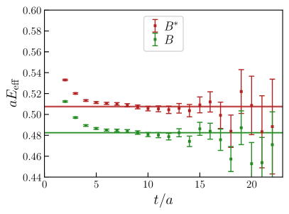
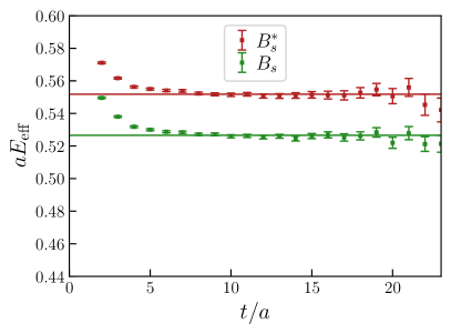
Figure 1: Effective energies of pseudoscalar and vector $B$ and $B_{s}$ mesons computed on ensemble a12m220L. Horizontal lines represent the corresponding final energies listed in Table 4.

Note that, due to the use of NRQCD, the energies listed in Table 4 and elsewhere contain overall negative shifts proportional to $n_{b}$, the number of $b$ quarks present in the corresponding states. At tree-level, this shift amounts to $-n_{b}m_{b}$, where $m_{b}$ is the $b$-quark mass. When considering energy differences between four-quark states and meson-meson thresholds with the same number of $b$ quarks, as done, for example, in Section V, these energy shifts cancel. Further quantities that can directly be compared to their experimental counterparts are the energy differences between the vector and pseudoscalar $B$ and $B_{s}$ meson energies. Experimentally, these differences are $E_{B^{\ast}}-E_{B}=45.21(21)\,\text{MeV}$ and $E_{B_{s}^{\ast}}-E_{B_{s}}=48.5^{+1.8}_{-1.5}\,\text{MeV}$ [69]. Our corresponding lattice results are listed in Table 4 and are found to be approximately 10% smaller. This discrepancy is likely due to the missing one-loop corrections to the matching coefficient $c_{4}$ of the term $-g/(2m_{b})\,\psi^{\dagger}\bm{\sigma}\cdot\mathbf{B}\psi$ in the NRQCD action.

We also determined the kinetic meson masses $m_{M,\,{\rm kin}}$ for $M\in\{B,B^{\ast},B_{s},B_{s}^{\ast}\}$, in which the energy shifts are not present, and which reflect the energy-momentum dispersion relation. The kinetic meson masses are important for scattering analyses, as discussed in Section VI. To determine them, we additionally computed the meson energies for several non-vanishing momenta, using the interpolating operators (14) to (17) with $\textbf{p}=2\pi\mathbf{n}/L$ with $\mathbf{n}\in\{(1,0,0),(1,1,0),(1,1,1),(2,0,0)\}$. Then we extracted $m_{M,\,{\rm kin}}$ by fitting the right-hand side of

$$E_{M}(\textbf{p})-E_{M}(0)=\sqrt{m_{M,\,{\rm kin}}^{2}+\textbf{p}^{2}}-m_{M,\,{\rm kin}}$$ (18)

for each $M\in\{B,B^{\ast},B_{s},B_{s}^{\ast}\}$ and each ensemble to the corresponding lattice results for the four energy differences $E_{M}(\textbf{p})-E_{M}(0)$. An exception are the three ensembles a12m220S, a12m220 and a12m220L, which only differ in the volume, and where we determined a common kinetic mass by performing a single fit for each meson to the corresponding twelve energy differences. The results for the kinetic masses are collected in Table 5. Moreover, in Fig. 2 we present an example plot demonstrating that the energy-momentum relation (18) is fully consistent with the data.

ensemble	$am_{B,\textrm{kin}}$	$am_{B^{*},\textrm{kin}}$	$am_{B_{s},\textrm{kin}}$	$am_{B_{s}^{*},\textrm{kin}}$
a15m310	$4.015(47)\phantom{0}$	$4.017(55)\phantom{0}$	$4.100(24)\phantom{0}$	$4.100(30)\phantom{0}$
a12m310	$3.224(96)\phantom{0}$	$3.238(108)$	$3.264(49)\phantom{0}$	$3.266(57)\phantom{0}$
a12m220S, a12m220, a12m220L	$3.121(84)\phantom{0}$	$3.091(89)\phantom{0}$	$3.233(37)\phantom{0}$	$3.204(40)\phantom{0}$
a09m310	$2.381(55)\phantom{0}$	$2.382(60)\phantom{0}$	$2.426(31)\phantom{0}$	$2.427(35)\phantom{0}$
a09m220	$2.342(161)$	$2.341(214)$	$2.397(79)\phantom{0}$	$2.399(94)\phantom{0}$

Table 5: Kinetic masses of the pseudoscalar and vector $B$ and $B_{s}$ mesons.

Figure 2: The $B$-meson energies for ensembles a12m220S, a12m220, and a12m220L as function of $(a\textbf{p})^{2}$, together with the fit using Eq. (18).

V Energies of antiheavy-antiheavy-light-light four-quark systems

To determine the low-lying energy levels for the $\bar{b}\bar{b}ud$ and $\bar{b}\bar{b}us$ four-quark systems from the $5\times 5$ and $7\times 7$ correlation matrices $C_{jk}(t)$ discussed in Section III.1.4, we solve the standard generalized eigenvalue problems (GEVPs)

$$\sum_{k}C_{jk}(t)v_{k,n}(t,t_{0})=\lambda_{n}(t,t_{0})\sum_{k}C_{jk}(t_{0})v_{k,n}(t,t_{0}),$$ (19)

where the indices $j$ and $k$ are operator indices and the indices $n$ enumerate the resulting eigenvalues and eigenvectors and are, thus, related to the indices of the low-lying energy eigenstates. The choice of $t_{0}$ is made individually for each system and each ensemble. Our strategy was to choose the largest value of $t_{0}$ for which statistical uncertainties on the resulting eigenvalues and eigenvectors did not significantly increase (see Table 6). The energy levels $E_{n}$ are then determined by carrying out a correlated $\chi^{2}$-minimizing fit of an exponential function to each resulting eigenvalue $\lambda_{n}(t,t_{0})$. Below, we also discuss the components $v_{j,n}(t,t_{0})$, where we always normalize the eigenvectors according to $\sum_{j}|v_{j,n}(t,t_{0})|^{2}=1$.

ensemble	$t_{0}/a$ for $\bar{b}\bar{b}ud$		$t_{0}/a$ for $\bar{b}\bar{b}us$
a15m310	2		2
a12m310, a12m220L, a12m220, a12m220S	3		3
a09m310, a09m220	4		6

Table 6: The $t_{0}$ values used for the GEVPs.

V.1 $\bar{b}\bar{b}ud$ energy levels

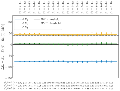
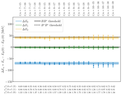
       ensemble a12m220S

       ensemble a12m220

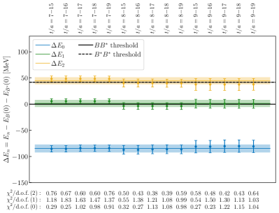
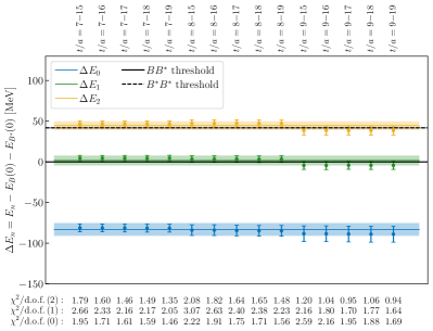
       ensemble a09m310

       ensemble a09m220

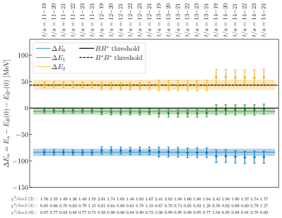
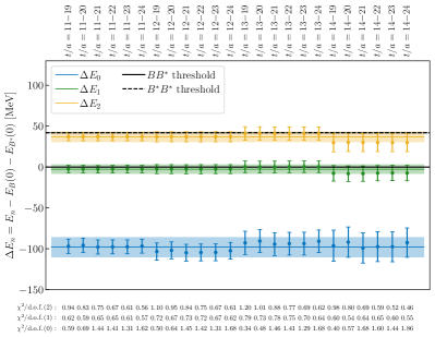
Figure 14: Fit ranges and fit results for the energy levels for the $\bar{b}\bar{b}ud$ system for the other ensembles.

As done in our determination of $B$ and $B_{s}$ meson energies in Section IV, we again consider multiple fit ranges $t_{\text{min}}\leq t\leq t_{\text{max}}$ by varying $t_{\text{min}}$ and $t_{\text{max}}$. For ensemble a12m220L, the fits are summarized in a graphical way in Fig. 3, including the corresponding fit ranges and resulting energy levels. Analogous plots for the other ensembles are collected in Fig. 14 in the appendix. As before, the final results are then generated by weighted averaging over all fits according to the FLAG method and are shown in Table 7 and Fig. 4, where $\Delta E_{n}=E_{n}-E_{B}(0)-E_{B^{\ast}}(0)$.

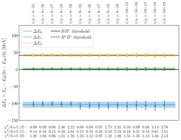
Figure 3: Fit ranges and fit results for the extraction of energy levels for the $\bar{b}\bar{b}ud$ system for ensemble a12m220L. The $BB^{\ast}$ and $B^{\ast}B^{\ast}$ thresholds correspond to the $B$ and $B^{\ast}$ energies obtained on that ensemble (see Table 4).

	$\Delta E_{0}$ [MeV]	$\Delta E_{1}$ [MeV]	$\Delta E_{2}$ [MeV]
a15m310	$\phantom{0}-75.5(1.8)\phantom{0}$	$\phantom{+}2.7(2.2)$	$45.2(2.5)$
a12m310	$\phantom{0}-70.1(4.2)\phantom{0}$	$-1.8(3.8)$	$40.5(4.2)$
a12m220S	$\phantom{0}-84.7(6.5)\phantom{0}$	$\phantom{+}1.9(5.3)$	$45.1(5.9)$
a12m220	$\phantom{0}-83.1(5.2)\phantom{0}$	$\phantom{+}2.5(3.7)$	$45.2(3.9)$
a12m220L	$-104.0(6.8)$	$\phantom{+}1.4(3.5)$	$42.1(3.7)$
a09m310	$\phantom{0}-83.8(5.9)\phantom{0}$	$-6.2(5.0)$	$44.1(6.2)$
a09m220	$\phantom{0}-98.1(9.6)\phantom{0}$	$-2.5(5.0)$	$37.1(5.5)$

Table 7: Finite-volume energy levels for the $\bar{b}\bar{b}ud$ system with respect to the $BB^{\ast}$ threshold, $\Delta E_{n}=E_{n}-E_{B}(0)-E_{B^{\ast}}(0)$.

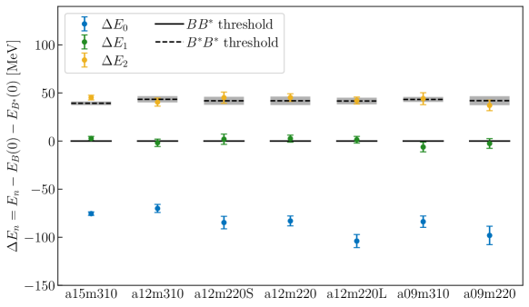
Figure 4: The three lowest finite-volume energy levels for the $\bar{b}\bar{b}ud$ system with $I(J^{P})=0(1^{+})$ obtained from our operator basis on each ensemble relative to the $BB^{*}$ threshold, $\Delta E_{n}=E_{n}-E_{B}(0)-E_{B^{\ast}}(0)$. The black horizontal lines correspond to the $BB^{*}$ (solid) and $B^{*}B^{*}$ (dashed) thresholds.

The ground-state energy is found to be significantly below the $BB^{\ast}$ threshold on all ensembles, $\Delta E_{0}\approx(-105\ldots\mbox{-70})$ MeV. An energy level in that region is expected from and consistent with previous lattice QCD investigations of this $\bar{b}\bar{b}ud$ system [38, 39, 40, 41, 43, 44]. It signals the existence of a QCD-stable $\bar{b}\bar{b}ud$ tetraquark. The energies of the first and second excitations are within statistical uncertainties consistent with the $BB^{\ast}$ and $B^{\ast}B^{\ast}$ thresholds. This indicates that, with our basis of interpolating operators, we are able to not only resolve the tetraquark state, but also these two low-lying scattering states.

As expected, with the operator basis used here [Eqs. (1) to (5)], we are not able to resolve scattering states with non-vanishing relative momenta. In particular, this is the case for $BB^{\ast}$ states in which the two mesons have opposite minimal non-vanishing momenta $p_{\text{min}}=(2\pi)/L$, where $L=N_{s}a$ is the ensemble-dependent spatial extent of the lattice. The estimated energy of such states with respect to the $BB^{\ast}$ threshold is

$$\Delta E_{BB^{\ast},p=p_{\text{min}}}=\Big{(}m_{B}^{2}+p_{\text{min}}^{2}\Big{)}^{1/2}+\Big{(}m_{B^{\ast}}^{2}+p_{\text{min}}^{2}\Big{)}^{1/2}-m_{B}-m_{B^{\ast}},$$ (20)

where $m_{B}$ and $m_{B^{\ast}}$ are the full meson masses, which can be taken to be the kinetic masses from Table 5. For example, for ensembles a12m220 and a12m220L, $\Delta E_{BB^{\ast},p=p_{\text{min}}}\approx 20\,\text{MeV}$ and $\Delta E_{BB^{\ast},p=p_{\text{min}}}\approx 13\,\text{MeV}$, respectively. With exception of ensemble a15m310, where $\Delta E_{BB^{\ast},p=p_{\text{min}}}\approx 50\,\text{MeV}$, we have $\Delta E_{BB^{\ast},p=p_{\text{min}}}<m_{B^{\ast}}-m_{B}\approx 45\,\text{MeV}$. Thus, the true second excited state is expected significantly below the $B^{\ast}B^{\ast}$ threshold, which is not reflected by the numerically obtained energy differences $\Delta E_{2}$ (see Table 7). The overlaps of our operators with this state are likely very small. To resolve this state and higher states of this type, we would need to include scattering operators with non-vanishing relative momenta.

To illustrate the importance of scattering operators, we compare in Fig. 5 effective energies obtained by solving GEVPs for a $3\times 3$ correlation matrix with only local operators [Eqs. (1) to (3)] (left plot) and the full $5\times 5$ correlation matrix, which also contains the scattering operators [Eqs. (4) and (5)] (right plot). While the effective masses $E_{\text{eff},1}(t)$ and $E_{\text{eff},2}(t)$, defined as $E_{\text{eff},n}(t)=(1/a)\ln(\lambda_{n}(t,t_{0})/\lambda_{n}(t+a,t_{0}))$, quickly approach the $BB^{\ast}$ and $B^{\ast}B^{\ast}$ thresholds for the full $5\times 5$ matrix, this is not the case for the $3\times 3$ matrix. Thus, it is practically impossible to extract physically meaningful energy levels $E_{n}$ for $n\geq 1$ from the $3\times 3$ matrix. The conclusion is that it is imperative to include scattering operators if energy levels of scattering states are needed, e.g., for a finite-volume scattering analysis as discussed in Section VI. However, the results for the effective energy $E_{\text{eff},0}(t)$ are essentially the same with and without scattering operators. Thus, if one is only interested in determining the mass of the QCD-stable $\bar{b}\bar{b}ud$ tetraquark in a finite volume, local operators may be sufficient. This finding is surprising, given our experience in Refs. [40, 42], where we compared multi-exponential matrix fits with and without scattering operators at the sink and found some impact on the fit results for $E_{0}$. In Refs. [40, 42], we were unable to use the GEVP for the non-square correlation matrices with scattering operators included at the sink only.

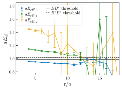
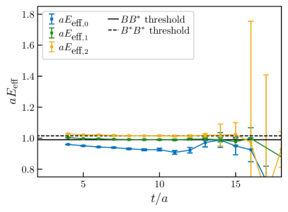
Figure 5: Effective energies $E_{\text{eff},n}(t)$, $n=0,1,2$ for the $\bar{b}\bar{b}ud$ system (ensemble a12m220L). Left: $3\times 3$ correlation matrix with only local interpolating operators [Eqs. (1) to (3)]. Right: $5\times 5$ correlation matrix including also scattering interpolating operators [Eqs. (4) and (5)].

The eigenvectors $v_{j,n}(t,t_{0})$ obtained by solving GEVPs are fairly independent of $t$ for larger $t$ and provide information about the composition of the low-lying energy eigenstates associated with the extracted energy levels $E_{n}$. In Fig. 6 we show the signed squared eigenvector components, $\text{sign}(\tilde{v}_{j,n})|\tilde{v}_{j,n}|^{2}$, for the full $5\times 5$ correlation matrix from ensemble a12m220L, where the quantities $\tilde{v}_{j,n}$ are obtained by fitting constants to $v_{j,n}(t,t_{0})$ in the range $t_{\text{min}}\leq t\leq t_{\text{max}}$ (we use multiple fits with different ranges, $6\leq t_{\text{min}}/a\leq 9$ and $12\leq t_{\text{max}}/a\leq 14$ in this case, and present the FLAG-method averages over these fits). When ignoring the signs, these quantities add up to 1 and can be interpreted as the relative importance of each interpolating operator $\mathcal{O}_{j}$ when approximating the energy eigenstate $|n\rangle$ as a sum over trial states $\mathcal{O}_{j}|n\rangle$ . The signs are of particular interest in the $\bar{b}\bar{b}us$ case (see Section V.2), where they expose the approximate light flavor symmetry of $u$ and $s$ quarks.

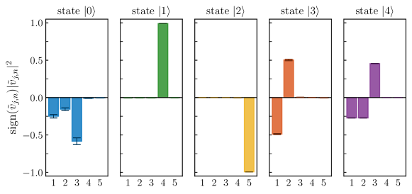
Figure 6: Signed squared eigenvector components, $\text{sign}(\tilde{v}_{j,n})|\tilde{v}_{j,n}|^{2}$, from ensemble a12m220L.

The results support our above conclusions based on the extracted energy levels. The ground state $|0\rangle$, which is a QCD-stable tetraquark, is excited almost exclusively by the three local operators [Eqs. (1) to (3)], while the scattering operators [Eqs. (4) and (5)] are essentially irrelevant. The relative contributions of the local operators to the QCD-stable tetraquark are, moreover, consistent with previous lattice QCD investigations using static potentials and the Born-Oppenheimer approximation. In particular, the $BB^{\ast}$ component is slightly larger than, but of similar magnitude as the $B^{\ast}B^{\ast}$ component, which is in agreement with Fig. 3 of Ref. [37], and the meson-meson components are of similar importance as the diquark-antidiquark component, which is in line with the main result from Ref. [66]. The first and second excitation $|1\rangle$ and $|2\rangle$, on the other hand, are clearly $BB^{\ast}$ and $B^{\ast}B^{\ast}$ scattering states, as already indicated by the consistency of their energy levels with the corresponding thresholds.

V.2 $\bar{b}\bar{b}us$ energy levels

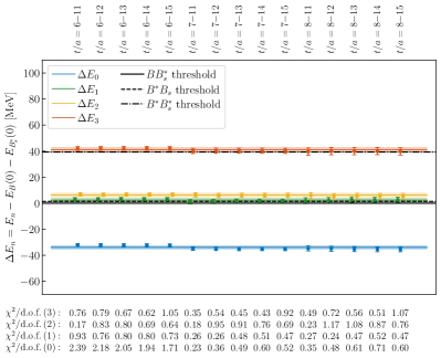
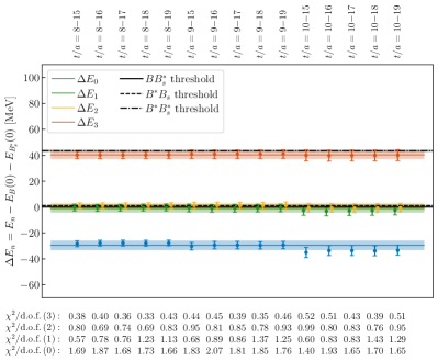
       ensemble a12m220S

       ensemble a12m220

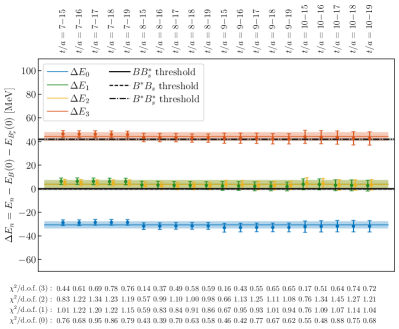
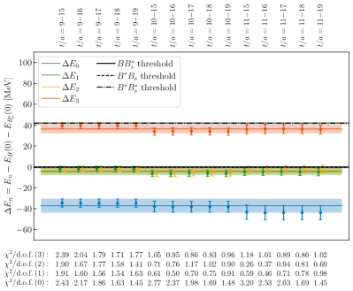
       ensemble a09m310

       ensemble a09m220

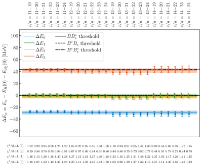
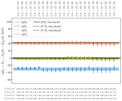
Figure 15: Fit ranges and fit results for the energy levels for the $\bar{b}\bar{b}us$ system for the other ensembles.

For the $\bar{b}\bar{b}us$ system we proceed in the same way as for the $\bar{b}\bar{b}ud$ system in Section V.1. For ensemble a12m220L, the fits are summarized in Fig. 7; the plots for the other ensembles are collected in Fig. 15 in the appendix. The final results for $\Delta E_{n}=E_{n}-E_{B}(0)-E_{B_{s}^{\ast}}(0)$ from the FLAG-method weighted averages are shown in Table 8 and Fig. 8.

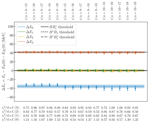
Figure 7: Fit ranges and fit results for the extraction of energy levels for the $\bar{b}\bar{b}us$ system for ensemble a12m220L. The $BB_{s}^{\ast}$, $B_{s}B^{\ast}$ and $B^{\ast}B_{s}^{\ast}$ thresholds correspond to the $B_{(s)}$ and $B_{(s)}^{\ast}$ energies obtained on that ensemble (see Table 4).

The ground-state energy is found to be significantly below the $BB_{s}^{\ast}$ threshold, $\Delta E_{0}\approx(-35\ldots-30)\text{MeV}$, indicating the existence of a QCD-stable $\bar{b}\bar{b}us$ tetraquark, consistent with previous lattice-QCD investigations of this system [38, 39, 42, 43]. We obtain precise results also for three additional states with energies consistent with the $BB_{s}^{\ast}$, $B_{s}B^{\ast}$ and $B^{\ast}B_{s}^{\ast}$ thresholds. However, as already noted for the $\bar{b}\bar{b}ud$ case, we are unable to resolve scattering states with non-vanishing back-to-back momenta; for example, on ensembles a12m220 and a12m220L one has $\Delta E_{BB_{s}^{\ast},p=p_{\text{min}}}\approx 20\,\text{MeV}$ and $\Delta E_{BB_{s}^{\ast},p=p_{\text{min}}}\approx 13\,\text{MeV}$, respectively. Scattering operators with non-vanishing back-to-back momenta would be needed to resolve these states.

	$\Delta E_{0}$ [MeV]	$\Delta E_{1}$ [MeV]	$\Delta E_{2}$ [MeV]	$\Delta E_{3}$ [MeV]
a15m310	$-34.0(1.2)$	$\phantom{+}2.4(1.4)$	$\phantom{+}6.2(1.5)$	$41.2(1.7)$
a12m310	$-29.6(2.5)$	$-1.0(2.7)$	$\phantom{+}0.7(2.4)$	$40.3(2.9)$
a12m220S	$-30.4(2.6)$	$\phantom{+}4.2(3.0)$	$\phantom{+}3.8(2.8)$	$44.5(3.2)$
a12m220	$-37.3(4.3)$	$-4.2(2.8)$	$-3.5(2.9)$	$36.6(3.2)$
a12m220L	$-35.8(3.2)$	$\phantom{+}0.6(2.3)$	$-0.1(2.2)$	$41.4(2.3)$
a09m310	$-29.1(2.5)$	$-1.1(2.7)$	$-2.4(2.6)$	$41.2(3.2)$
a09m220	$-30.7(4.0)$	$-1.3(3.0)$	$-2.1(3.3)$	$40.5(3.3)$

Table 8: Finite-volume energy levels for the $\bar{b}\bar{b}us$ system with respect to the $BB_{s}^{\ast}$ threshold, $\Delta E_{n}=E_{n}-E_{B}(0)-E_{B_{s}^{\ast}}(0)$.

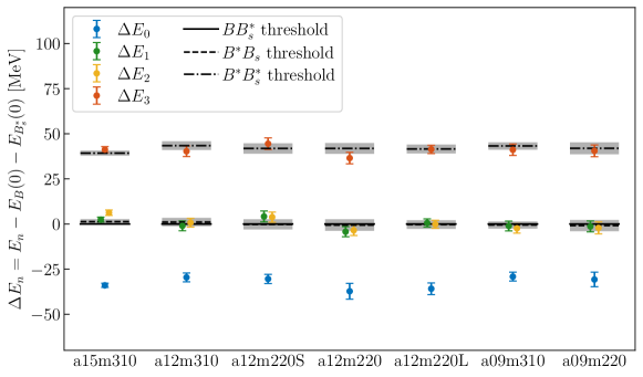
Figure 8: The four lowest finite-volume energy levels for the $\bar{b}\bar{b}us$ system with $J^{P}=1^{+}$ obtained from our operator basis on each ensemble relative to the $BB_{s}^{*}$ threshold, $\Delta E_{n}=E_{n}-E_{B}(0)-E_{B_{s}^{\ast}}(0)$. The black horizontal lines correspond to the $BB_{s}^{*}$ (solid), $B^{*}B_{s}$ (dashed) and $B^{*}B_{s}^{*}$ (dashed-dotted) thresholds.

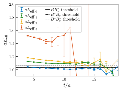
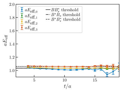
Figure 9: Effective energies $E_{\text{eff},n}(t)$, $n=0,1,2,3$ for $\bar{b}\bar{b}us$ (ensemble a12m220L). Left: $4\times 4$ correlation matrix with only local interpolating operators [Eqs. (6) to (9)]. Right: $7\times 7$ correlation matrix with also scattering interpolating operators [Eqs. (10) to (12)].

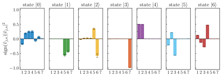
Figure 10: Signed squared eigenvector components, $\text{sign}(\tilde{v}_{j,n})|\tilde{v}_{j,n}|^{2}$, from ensemble a12m220L.

Again, we illustrate the importance of the scattering operators by comparing in Fig. 9 effective energies obtained by solving GEVPs for a $4\times 4$ correlation matrix with only local operators [Eqs. (6) to (9)] (left plot) and the full $7\times 7$ correlation matrix, which also contains the scattering operators [Eqs. (10) to (12)] (right plot). The overall picture and conclusions are the same as for the $\bar{b}\bar{b}ud$ system. To determine the mass of the QCD-stable $\bar{b}\bar{b}us$ tetraquark, local operators appear to be sufficient, but it is imperative to include scattering operators if energy levels of scattering states are needed. The fact that the results for $E_{\text{eff},0}(t)$ are essentially the same with and without scattering operators is even more surprising here than for the $\bar{b}\bar{b}ud$ system, given the weaker binding.

In Fig. 10 we show the signed squared eigenvector components $\text{sign}(\tilde{v}_{j,n})|\tilde{v}_{j,n}|^{2}$ for the full $7\times 7$ correlation matrix from ensemble a12m220L (here, we use the FLAG-method averages over fits with $5\leq t_{\text{min}}/a\leq 9$ and $11\leq t_{\text{max}}/a\leq 14$). The eigenvector components support and complement our above conclusions based on the extracted energy levels, and exhibit the approximate SU(3) flavor symmetry. The ground state $|0\rangle$, which is a QCD-stable tetraquark, is excited mostly by the four local operators. It is $us$ flavor antisymmetric, which shows that the $\bar{b}\bar{b}us$ tetraquark has a flavor structure analogous the $I=0$ $\bar{b}\bar{b}ud$ tetraquark discussed in the previous section. The first and second excitations are mixtures of $BB_{s}^{\ast}$ and $B_{s}B^{\ast}$ scattering states, where $|1\rangle$ is mostly $us$ flavor symmetric, i.e. similar to $I=1$, while $|2\rangle$ is mostly $us$ flavor antisymmetric, i.e. similar to $I=0$. The third excitation $|3\rangle$ is clearly a $B^{\ast}B_{s}^{\ast}$ scattering state, as already suggested by its energy.

VI Finite-volume effects

Some of the previous lattice-QCD studies of $\bar{b}\bar{b}ud$ and $\bar{c}\bar{c}ud$ systems [40, 70, 71] have employed Lüscher’s method [52, 72, 73, 74, 75, 76, 77, 78, 79, 53] to relate the finite-volume energy levels with infinite-volume $B$-$B^{*}$ and $D$-$D^{*}$ scattering amplitudes. The masses of the infinite-volume bound states or virtual bound states were then obtained as the pole locations in these amplitudes. Such an analysis has not yet been performed for the $\bar{b}\bar{b}us$ system, which is more challenging due to the coupling of the $B_{s}$-$B^{*}$ and $B$-$B_{s}^{*}$ channels with nearly identical thresholds [42]. The improvements made in the present work in extracting the finite-volume spectra (compared to Refs. [40, 42]) in principle enable more advanced scattering-amplitude analyses, including an analysis of coupled-channel $B_{s}$-$B^{*}$, $B$-$B_{s}^{*}$ scattering.

The studies presented in Refs. [40, 70, 71] used Lüscher’s method both above and below threshold, and used effective-range expansions (EREs) to parametrize the energy dependence of the scattering amplitude. It was recently pointed out that the $D$-$D^{*}$ scattering amplitude has a left-hand cut starting close to threshold due to pion exchange [80], which determines the radius of convergence of the ERE to be smaller than the regions studied in the aforementioned references. The same problem is also present in $B$-$B^{*}$ scattering and, due to kaon exchange, in $B_{s}$-$B^{*}$, $B$-$B_{s}^{*}$ scattering. Moreover, the two-body Lüscher quantization condition itself becomes invalid on the left-hand cut  [81, 82, 83, 84, 85, 86, 87].

For $B$-$B^{*}$ scattering, the left-hand cut due to single-pion exchange starts at the invariant-mass-squared

$$s_{\rm cut}=s_{\rm th}-m_{\pi}^{2}+(m_{B^{*}}-m_{B})^{2},$$ (21)

where $s_{\rm th}=(m_{B^{*}}+m_{B})^{2}$. For physical pion mass, one finds $\sqrt{s_{\rm cut}}-\sqrt{s_{\rm th}}\approx-1\>{\rm MeV}$, while at $m_{\pi}=300\>{\rm MeV}$, $\sqrt{s_{\rm cut}}-\sqrt{s_{\rm th}}\approx-4\>{\rm MeV}$. Similarly, for $B_{s}$-$B^{*}$, $B$-$B_{s}^{*}$ scattering at physical kaon mass, the cut due to single-kaon exchange starts at $\sqrt{s_{\rm cut}}-\sqrt{s_{\rm th}}\approx-11\>{\rm MeV}$. The finite-volume ground-state energies we obtained in this work (Section V) and in Refs. [40, 42] for $\bar{b}\bar{b}ud$ and $\bar{b}\bar{b}us$ are well below these values.

New approaches to describing the finite-volume energy levels in the region effected by the left-hand cut were recently proposed in Refs. [81, 82, 83, 84, 85, 86, 87]; these involve modifications to the two-body Lüscher formalism, the use of the three-body Lüscher formalism, or chiral effective theory. However, the implementation of these approaches is beyond the scope of the present work.

In the remainder of this paper, we will focus on the ground-state energies and assume that finite-volume effects are negligible compared to our statistical uncertainties. Before we became aware of the left-hand cut problem, we did in fact perform extractions of $S$-wave scattering amplitudes from the energy levels presented here using the standard two-body Lüscher method; we can use these results to get at least some idea of the possible size of finite-volume effects. For the $\bar{b}\bar{b}ud$ system, we used the lowest two energy levels on each ensemble and fitted a two-parameter model of the $K$ matrix [88], similar to the effective-range expansion used in [40]. From these fits, we found that the bound-state pole locations differ from the finite-volume ground-state energies by $\lesssim 0.1$ MeV, consistent with the expectation from Ref. [40]. For $\bar{b}\bar{b}us$, we attempted coupled-channel fits to the lowest three energy levels with various parametrizations of the $2\times 2$ $K$ matrix, including fits that combine the data from the a12m220S, a12m220, and a12m220L ensembles that differ only in the volume. However, most of these fits did not converge properly, and the only model that gave stable results was a diagonal form of the $K$ matrix with two $s$-independent parameters on the diagonal. For those ensembles for which we achieved a reasonable $\chi^{2}/{\rm d.o.f}$, this model predicted shifts between the finite-volume ground-state energies and the bound-state pole locations of $\lesssim 1$ MeV. Another way of estimating the finite-volume effects is directly comparing the finite-volume energies of the a12m220S, a12m220, and a12m220L ensembles listed in Table 8, which suggests that the effects for $\bar{b}\bar{b}us$ are not larger than about 5 MeV for the smallest volume.

VII Chiral and continuum extrapolations of the binding energies

To obtain estimates of the tetraquark binding energies at the physical point, we consider two different fits to the ground-state energies from the different ensembles: (i) neglecting lattice-spacing dependence but allowing for a linear dependence on $m_{\pi}^{2}$, as in Refs. [40, 42],

$$\Delta E_{0}(m_{\pi})=\Delta E_{0}(m_{\pi,\text{phys}})+c(m_{\pi}^{2}-m_{\pi,\text{phys}}^{2}),$$ (22)

and (ii), allowing for linear dependencies on both $m_{\pi}^{2}$ and $a^{2}$,

$$\Delta E_{0}(m_{\pi},a)=\Delta E_{0}(m_{\pi,\text{phys}},0)+c(m_{\pi}^{2}-m_{\pi,\text{phys}}^{2})+d\,a^{2}.$$ (23)

Here, we use $m_{\pi,\text{phys}}=135\,\textrm{MeV}$ for the physical pion mass in the isospin-symmetric limit. These models are expected to be approximate only. For the actions used here, gluon and sea-quark discretization errors are expected to start at $O(\alpha_{s}^{2}a^{2})$ and $O(\alpha_{s}a^{2})$, respectively, but the Wilson-clover valence action is only tree-level-$O(a)$ improved and thus will have some remaining $O(\alpha_{s}a)$ errors. With the particular level of Symanzik improvement used here, the NRQCD action has both $O(\alpha_{s}^{2}a)$ and $O(\alpha_{s}^{2}a^{2})$ errors, plus other systematic errors from missing higher-order relativistic and radiative corrections that we will estimate separately below.

Our fits using Eqs. (22) or (23) are illustrated in Figs. 11 and 12, and the results for the fit parameters are given in Table 9. The coefficients $d$ that describe the lattice-spacing dependence turn out to be consistent with zero. For the $\bar{b}\bar{b}ud$ system, there is a slight indication that the binding energy increases in magnitude as the pion mass is lowered, which becomes more statistically significant when not including the $a^{2}$ term. On the other hand, the $\bar{b}\bar{b}us$ binding energy is essentially independent of the pion mass in the range considered here. Some of the fits have $\chi^{2}/\textrm{d.o.f.}>1$ due to a slight tension between data points with similar lattice parameters; in these cases, we scaled the uncertainties of the fit results by $\sqrt{\chi^{2}/\textrm{d.o.f.}}$. We find that the results for $\Delta E_{0}(m_{\pi,\text{phys}})$ and $\Delta E_{0}(m_{\pi,\text{phys}},0)$ are compatible within statistical uncertainties. We take the latter as our final estimates of the tetraquark binding energies.

The extrapolations do not remove the systematic errors from missing higher-order relativistic and radiative corrections in the lattice NRQCD action. To estimate these sources of systematic uncertainty, we follow the prescription of Ref. [40] with adjustments for the different choices of NRQCD matching coefficients used here.

The values of $\Delta E_{0}$ depend both on the heavy-light meson energies and on the energies of the four-quark systems. For the heavy-light mesons, the most significant systematic NRQCD uncertainties are expected to be as follows:

• Four-quark operators are missing in the action. They appear only at order $\alpha_{s}^{2}$ in the QCD matching, but according to Ref. [89] their effect is of order $3\,{\rm MeV}$.

• One-loop corrections to the matching coefficient $c_{4}$ of the operator $-g/(2m_{b})\,\psi^{\dagger}\bm{\sigma}\cdot\mathbf{B}\psi$ are not included here. The associated uncertainties can be estimated as

  $$\alpha_{s}\Lambda_{\textrm{QCD}}^{2}/m_{b}\approx 6\,{\rm MeV},$$ (24)

  where we use $\alpha_{s}\approx 0.3$, $\Lambda_{\textrm{QCD}}\approx 300$ MeV, and $m_{b}\approx 4.5$ GeV.

• We also use only tree-level values for the coefficients $c_{2}$ and $c_{3}$ of the operators of order $(\Lambda_{\textrm{QCD}}^{2}/m_{b}^{2})$. The uncertainties from missing higher-order contributions to these coefficients are given by

  $$\alpha_{s}\Lambda_{\textrm{QCD}}^{3}/m_{b}^{2}\approx 0.4\,{\rm MeV}.$$ (25)

As the matching coefficients $c_{1}$, $c_{5}$, and $c_{6}$ include order-$\alpha_{s}$ corrections, systematic uncertainties arising from the related operators are negligible.

For the four-quark system, the power counting is more complicated due to the presence of two bottom quarks. A reasonable estimate for the systematic uncertainties can be obtained by replacing the QCD scale $\Lambda_{\textrm{QCD}}$ by the binding momentum $|k_{\textrm{BS}}|$ (if larger than $\Lambda_{\textrm{QCD}}$) [40]. Our results for the binding energies correspond to $|k_{\textrm{BS}}|\approx 730$ MeV for $\bar{b}\bar{b}ud$ and $|k_{\textrm{BS}}|\approx 400$ MeV for $\bar{b}\bar{b}us$, which leads to estimated systematic uncertainties of $\approx 36$ MeV for the $\bar{b}\bar{b}ud$ energy and $\approx 11$ MeV for the $\bar{b}\bar{b}us$ energy. It is reasonable to expect some partial cancellation of systematic errors between the tetraquark and heavy-light meson energies, so these numbers could be taken as the total systematic uncertainties of $\Delta E_{0}$ [40]. However, note that our previous calculations [40, 42] predicted larger binding momenta of $|k_{\textrm{BS}}|\approx 800$ MeV for $\bar{b}\bar{b}ud$ and $|k_{\textrm{BS}}|\approx 680$ MeV for $\bar{b}\bar{b}us$, and the smaller values obtained here may, in principle, be due to the very systematic errors we are trying to estimate. Therefore, to be conservative, we will report asymmetric uncertainties in which we use the larger values of $|k_{\textrm{BS}}|$ from Refs. [40, 42] to obtain the size of the error bars in the direction of increased binding. This prescription then yields our final results

$$\Delta E_{0}(m_{\pi,\text{phys}},0)[\bar{b}\bar{b}ud] = -100\pm 10\>^{+36}_{-43}\>\>{\rm MeV},$$ (26)

$$\Delta E_{0}(m_{\pi,\text{phys}},0)[\bar{b}\bar{b}us] = -30\pm 3\>^{+11}_{-31}\>\>{\rm MeV}.$$ (27)

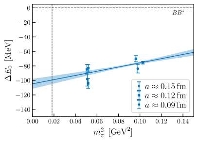
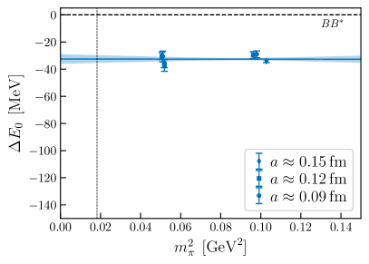
Figure 11: Chiral extrapolations of the energy differences $\Delta E_{0}$ for the $\bar{b}\bar{b}ud$ four-quark system with $I(J^{P})=0(1^{+})$ (left) and the $\bar{b}\bar{b}us$ four-quark system with $J^{P}=1^{+}$(right), neglecting the lattice-spacing dependence. The lowest meson-meson threshold for each channel is indicated by the horizontal dashed lines, while the vertical dashed line represents the physical pion mass.

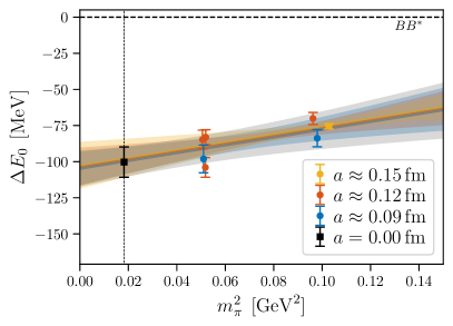
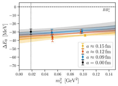
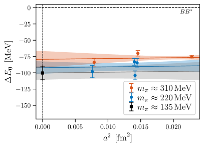
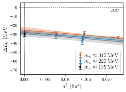
Figure 12: Combined chiral and continuum extrapolations of the energy differences $\Delta E_{0}$ for the $\bar{b}\bar{b}ud$ four-quark system with $I(J^{P})=0(1^{+})$ (left) and the $\bar{b}\bar{b}us$ four-quark system with $J^{P}=1^{+}$(right). In the upper row, the $m_{\pi}$ dependence is shown for fixed lattice spacing $a$, while the lower row shows the $a$ dependence for fixed pion mass $m_{\pi}$. The lowest meson-meson threshold for each channel is indicated by the horizontal dashed lines, while the vertical dashed line represents either the physical pion mass or zero lattice spacing $a$. The black square indicates the final result for the binding energy at the physical point.

Chiral extrapolation only
	$\Delta E_{0}(m_{\pi,\textrm{phys}})$ [MeV]	$c$ [$10^{-4}$/MeV]		$\chi^{2}/\textrm{d.o.f.}$
$\bar{b}\bar{b}ud$	$-99(8)$	$2.9(1.1)$		$2.34$
$\bar{b}\bar{b}us$	$-33(4)$	$0.0(0.5)$		$1.57$
Chiral and continuum extrapolation
	$\Delta E_{0}(m_{\pi,\textrm{phys}},0)$ [MeV]	$c$ [$10^{-4}$/MeV]	$d$ [$10^{2}\times$MeV3]	$\chi^{2}/\textrm{d.o.f.}$
$\bar{b}\bar{b}ud$	$-100(10)$	$2.7(1.6)$	$1.2(6.2)$	$2.90$
$\bar{b}\bar{b}us$	$-30(3)\phantom{0}$	$0.5(0.5)$	$3.8(1.8)$	$0.83$

Table 9: Fit results for the chiral extrapolations using Eq. (22) [upper table] and the combined chiral-continuum extrapolations using Eq. (23) [lower table]. All uncertainties have been scaled by $\sqrt{\chi^{2}/\textrm{d.o.f.}}$.

VIII Conclusions

In this work, we have confirmed the existence and computed the binding energies of both the $\bar{b}\bar{b}ud$ tetraquark with quantum numbers $I(J^{P})=0(1^{+})$ and the $\bar{b}\bar{b}us$ tetraquark with quantum numbers $J^{P}=1^{+}$ using lattice QCD. We have improved on existing similar lattice-QCD computations [38, 39, 40, 41, 42, 43, 44] by implementing, for the first time, a combination of local and scattering interpolating operators both at the source and at the sink of symmetric correlation matrices. We have demonstrated that this enables high-precision determinations of the energies of low-lying scattering states, and that it is practically impossible to determine these energies without scattering operators. Reliably extracting the complete low-lying finite-volume spectra is essential when using the Lüscher method to determine energy-dependent scattering amplitudes, as we have done for the $\bar{b}\bar{c}ud$ systems with quantum numbers $I(J^{P})=0(0^{+})$ and $I(J^{P})=0(1^{+})$ in Ref. [49], based on the methods developed here. On the other hand, we found that the inclusion of scattering operators had essentially no impact on the ground-state results obtained from the GEVP for the $\bar{b}\bar{b}ud$ and $\bar{b}\bar{b}us$ systems. This finding was somewhat unexpected, given our experience from Refs. [40, 42], in which we compared the results of multi-exponential matrix fits with and without scattering operators at the sink and found some impact on the fit results for $E_{0}$. When using the GEVP, local operators alone appear to be sufficient to determine the binding energies of the deeply bound $\bar{b}\bar{b}ud$ and $\bar{b}\bar{b}us$ tetraquarks, but the inclusion of scattering operators provides reassurance and may be necessary to reliably extract the ground-state energies of other, less deeply bound systems.

Using chiral and continuum extrapolations of the results from several ensembles, we obtained binding energies of $-100\pm 10\>^{+36}_{-43}\>\>{\rm MeV}$ for the $\bar{b}\bar{b}ud$ tetraquark with quantum numbers $I(J^{P})=0(1^{+})$ and $-30\pm 3\>^{+11}_{-31}\>\>{\rm MeV}$ for the $\bar{b}\bar{b}us$ tetraquark with quantum numbers $J^{P}=1^{+}$. These values are reasonably consistent with results of other recent lattice-QCD studies of these systems [39, 40, 42, 43, 44], but are in slight tension with earlier works [38, 41]. We have updated the summary plots for both tetraquark systems from Refs. [40, 42] and show them in Fig. 13. For the $\bar{b}\bar{b}ud$ system, also calculations [33, 34, 37] based on static potentials from lattice QCD and the Born-Oppenheimer approximation are shown; these gave a somewhat smaller binding energy. The predictions from other approaches such as potential models, effective field theories, and QCD sum rules were taken from Refs. [1, 4, 5, 6, 7, 8, 9, 10, 11, 12, 13, 3, 14, 15, 16, 17, 18, 19, 20, 21, 22, 23, 24, 25, 26, 27, 28, 29, 30, 31, 32].

The main systematic uncertainties in our present results are associated with the lattice NRQCD action [64], in particular with the use of the tree-level value of the coefficient $c_{4}$ and the missing four-quark operators. The radiative corrections to $c_{2}$ and $c_{4}$, and the coefficients of the four-quark operators with four heavy quarks have in fact been computed to one loop in lattice perturbation theory in Refs. [90, 91]. The systematic uncertainties could have been reduced by including these corrections, although four-quark operators with both heavy and light quarks would still be missing. A computation of the $\bar{b}\bar{b}ud$ and $\bar{b}\bar{b}us$ tetraquark energies using a relativistic action for the $\bar{b}$ quarks is also a worthwhile future direction to complement and cross-check the results from this work and from Refs. [38, 39, 40, 41, 42, 43, 44], which all used NRQCD.

Finally, we note that the calculations presented here only used scattering interpolating operators with zero relative momenta, leading to missing states in the energy range considered, especially for the larger volumes. A natural next step is to include also scattering operators with non-vanishing relative momenta. Their implementation is straightforward within our computational setup, and we have already included such operators in our recent investigation of the $\bar{b}\bar{c}ud$ systems [49].

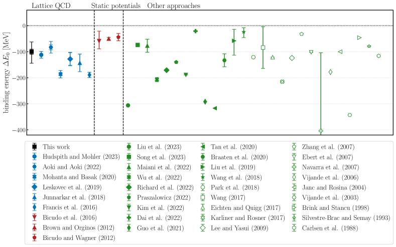
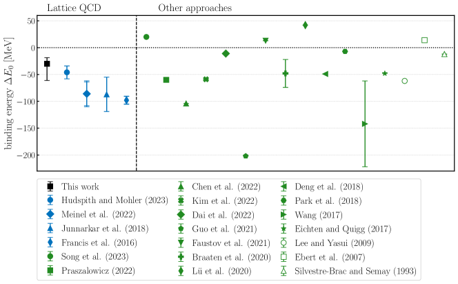
Figure 13: Comparison of results for the binding energy of antiheavy-antiheavy-light-light tetraquarks. (upper plot): $\bar{b}\bar{b}ud$ tetraquark with $I(J^{P})=0(1^{+})$ (black: this work; blue: previous full lattice-QCD simulations [38, 39, 40, 41, 43, 44]; red: lattice-QCD computations of static potentials in combination with the Born-Oppenheimer approximation [33, 34, 37]; green: other approaches (quark models, phenomenological considerations, sum rules [1, 4, 5, 6, 7, 8, 9, 10, 11, 12, 13, 3, 14, 15, 17, 18, 19, 23, 24, 25, 27, 28, 29, 30, 31, 32]). (lower plot): $\bar{b}\bar{b}us$ tetraquark with $J^{P}=1^{+}$ (black: this work; blue: previous full lattice-QCD simulations [38, 39, 42, 43]; green: other approaches (quark models, phenomenological considerations, sum rules [4, 10, 12, 3, 14, 15, 16, 20, 21, 22, 23, 24, 25, 26, 27, 31]).

Appendix A Additional plots for the other ensembles

       ensemble a15m310

       ensemble a12m310

       ensemble a15m310

       ensemble a12m310

References

- [1] J. Carlson, L. Heller, and J. A. Tjon, “Stability of Dimesons,” Phys. Rev. D 37 (1988) 744.
- [2] A. V. Manohar and M. B. Wise, “Exotic Q Q anti-q anti-q states in QCD,” Nucl. Phys. B 399 (1993) 17–33, arXiv:hep-ph/9212236.
- [3] E. J. Eichten and C. Quigg, “Heavy-quark symmetry implies stable heavy tetraquark mesons ,” Phys. Rev. Lett. 119 no. 20, (2017) 202002, arXiv:1707.09575 [hep-ph].
- [4] B. Silvestre-Brac and C. Semay, “Systematics of L = 0 q-2 anti-q-2 systems,” Z. Phys. C 57 (1993) 273–282.
- [5] D. M. Brink and F. Stancu, “Tetraquarks with heavy flavors,” Phys. Rev. D 57 (1998) 6778–6787.
- [6] J. Vijande, F. Fernandez, A. Valcarce, and B. Silvestre-Brac, “Tetraquarks in a chiral constituent quark model,” Eur. Phys. J. A 19 (2004) 383, arXiv:hep-ph/0310007.
- [7] D. Janc and M. Rosina, “The molecular state,” Few Body Syst. 35 (2004) 175–196, arXiv:hep-ph/0405208.
- [8] J. Vijande, A. Valcarce, and K. Tsushima, “Dynamical study of bf QQ - anti-u anti-d mesons,” Phys. Rev. D 74 (2006) 054018, arXiv:hep-ph/0608316.
- [9] F. S. Navarra, M. Nielsen, and S. H. Lee, “QCD sum rules study of QQ - anti-u anti-d mesons,” Phys. Lett. B 649 (2007) 166–172, arXiv:hep-ph/0703071.
- [10] D. Ebert, R. N. Faustov, V. O. Galkin, and W. Lucha, “Masses of tetraquarks with two heavy quarks in the relativistic quark model,” Phys. Rev. D 76 (2007) 114015, arXiv:0706.3853 [hep-ph].
- [11] M. Zhang, H. X. Zhang, and Z. Y. Zhang, “QQ anti-q anti-q four-quark bound states in chiral SU(3) quark model,” Commun. Theor. Phys. 50 (2008) 437–440, arXiv:0711.1029 [nucl-th].
- [12] S. H. Lee and S. Yasui, “Stable multiquark states with heavy quarks in a diquark model,” Eur. Phys. J. C 64 (2009) 283–295, arXiv:0901.2977 [hep-ph].
- [13] M. Karliner and J. L. Rosner, “Discovery of doubly-charmed baryon implies a stable () tetraquark,” Phys. Rev. Lett. 119 no. 20, (2017) 202001, arXiv:1707.07666 [hep-ph].
- [14] Z.-G. Wang, “Analysis of the axialvector doubly heavy tetraquark states with QCD sum rules,” Acta Phys. Polon. B 49 (2018) 1781, arXiv:1708.04545 [hep-ph].
- [15] W. Park, S. Noh, and S. H. Lee, “Masses of the doubly heavy tetraquarks in a constituent quark model,” Nucl. Phys. A 983 (2019) 1–19, arXiv:1809.05257 [nucl-th].
- [16] C. Deng, H. Chen, and J. Ping, “Systematical investigation on the stability of doubly heavy tetraquark states,” Eur. Phys. J. A 56 no. 1, (2020) 9, arXiv:1811.06462 [hep-ph].
- [17] B. Wang, Z.-W. Liu, and X. Liu, “ interactions in chiral effective field theory,” Phys. Rev. D 99 no. 3, (2019) 036007, arXiv:1812.04457 [hep-ph].
- [18] M.-Z. Liu, T.-W. Wu, M. Pavon Valderrama, J.-J. Xie, and L.-S. Geng, “Heavy-quark spin and flavor symmetry partners of the X(3872) revisited: What can we learn from the one boson exchange model?,” Phys. Rev. D 99 no. 9, (2019) 094018, arXiv:1902.03044 [hep-ph].
- [19] Y. Tan, W. Lu, and J. Ping, “Systematics of in a chiral constituent quark model,” Eur. Phys. J. Plus 135 no. 9, (2020) 716, arXiv:2004.02106 [hep-ph].
- [20] Q.-F. Lü, D.-Y. Chen, and Y.-B. Dong, “Masses of doubly heavy tetraquarks in a relativized quark model,” Phys. Rev. D 102 no. 3, (2020) 034012, arXiv:2006.08087 [hep-ph].
- [21] E. Braaten, L.-P. He, and A. Mohapatra, “Masses of doubly heavy tetraquarks with error bars,” Phys. Rev. D 103 no. 1, (2021) 016001, arXiv:2006.08650 [hep-ph].
- [22] R. N. Faustov, V. O. Galkin, and E. M. Savchenko, “Heavy tetraquarks in the relativistic quark model,” Universe 7 no. 4, (2021) 94, arXiv:2103.01763 [hep-ph].
- [23] T. Guo, J. Li, J. Zhao, and L. He, “Mass spectra of doubly heavy tetraquarks in an improved chromomagnetic interaction model,” Phys. Rev. D 105 no. 1, (2022) 014021, arXiv:2108.10462 [hep-ph].
- [24] L. R. Dai, E. Oset, A. Feijoo, R. Molina, L. Roca, A. M. Torres, and K. P. Khemchandani, “Masses and widths of the exotic molecular B(s)(*)B(s)(*) states,” Phys. Rev. D 105 no. 7, (2022) 074017, arXiv:2201.04840 [hep-ph]. [Erratum: Phys.Rev.D 106, 099904 (2022)].
- [25] Y. Kim, M. Oka, and K. Suzuki, “Doubly heavy tetraquarks in a chiral-diquark picture,” Phys. Rev. D 105 no. 7, (2022) 074021, arXiv:2202.06520 [hep-ph].
- [26] X. Chen, F.-L. Wang, Y. Tan, and Y. Yang, “Double-heavy tetraquarks with strangeness in the chiral quark model*,” Chin. Phys. C 47 no. 2, (2023) 023102, arXiv:2206.10917 [hep-ph].
- [27] M. Praszalowicz, “Doubly heavy tetraquarks in the chiral quark soliton model,” Phys. Rev. D 106 no. 11, (2022) 114005, arXiv:2208.08602 [hep-ph].
- [28] J.-M. Richard, A. Valcarce, and J. Vijande, “Doubly-heavy tetraquark bound states and resonances,” Nucl. Part. Phys. Proc. 324-329 (2023) 64–67, arXiv:2209.07372 [hep-ph].
- [29] T.-W. Wu and Y.-L. Ma, “Doubly heavy tetraquark multiplets as heavy antiquark-diquark symmetry partners of heavy baryons,” Phys. Rev. D 107 no. 7, (2023) L071501, arXiv:2211.15094 [hep-ph].
- [30] L. Maiani, A. Pilloni, A. D. Polosa, and V. Riquer, “Doubly heavy tetraquarks in the Born-Oppenheimer approximation,” Phys. Lett. B 836 (2023) 137624, arXiv:2208.02730 [hep-ph].
- [31] Y. Song and D. Jia, “Mass spectra of doubly heavy tetraquarks in diquarkantidiquark picture,” Commun. Theor. Phys. 75 no. 5, (2023) 055201, arXiv:2301.00376 [hep-ph].
- [32] X.-Y. Liu, W.-X. Zhang, and D. Jia, “Doubly heavy tetraquarks: Heavy quark bindings and chromomagnetically mixings,” Phys. Rev. D 108 no. 5, (2023) 054019, arXiv:2303.03923 [hep-ph].
- [33] P. Bicudo and M. Wagner, “Lattice QCD signal for a bottom-bottom tetraquark,” Phys. Rev. D 87 no. 11, (2013) 114511, arXiv:1209.6274 [hep-ph].
- [34] Z. S. Brown and K. Orginos, “Tetraquark bound states in the heavy-light heavy-light system,” Phys. Rev. D 86 (2012) 114506, arXiv:1210.1953 [hep-lat].
- [35] P. Bicudo, K. Cichy, A. Peters, and M. Wagner, “BB interactions with static bottom quarks from Lattice QCD,” Phys. Rev. D 93 no. 3, (2016) 034501, arXiv:1510.03441 [hep-lat].
- [36] P. Bicudo, K. Cichy, A. Peters, B. Wagenbach, and M. Wagner, “Evidence for the existence of and the non-existence of and tetraquarks from lattice QCD,” Phys. Rev. D 92 no. 1, (2015) 014507, arXiv:1505.00613 [hep-lat].
- [37] P. Bicudo, J. Scheunert, and M. Wagner, “Including heavy spin effects in the prediction of a tetraquark with lattice QCD potentials,” Phys. Rev. D 95 no. 3, (2017) 034502, arXiv:1612.02758 [hep-lat].
- [38] A. Francis, R. J. Hudspith, R. Lewis, and K. Maltman, “Lattice Prediction for Deeply Bound Doubly Heavy Tetraquarks,” Phys. Rev. Lett. 118 no. 14, (2017) 142001, arXiv:1607.05214 [hep-lat].
- [39] P. Junnarkar, N. Mathur, and M. Padmanath, “Study of doubly heavy tetraquarks in Lattice QCD,” Phys. Rev. D 99 no. 3, (2019) 034507, arXiv:1810.12285 [hep-lat].
- [40] L. Leskovec, S. Meinel, M. Pflaumer, and M. Wagner, “Lattice QCD investigation of a doubly-bottom tetraquark with quantum numbers ,” Phys. Rev. D 100 no. 1, (2019) 014503, arXiv:1904.04197 [hep-lat].
- [41] P. Mohanta and S. Basak, “Construction of tetraquark states on lattice with NRQCD bottom and HISQ up and down quarks,” Phys. Rev. D 102 no. 9, (2020) 094516, arXiv:2008.11146 [hep-lat].
- [42] S. Meinel, M. Pflaumer, and M. Wagner, “Search for and tetraquark bound states using lattice QCD,” Phys. Rev. D 106 no. 3, (2022) 034507, arXiv:2205.13982 [hep-lat].
- [43] R. J. Hudspith and D. Mohler, “Exotic tetraquark states with two b¯ quarks and JP=0+ and 1+ Bs states in a nonperturbatively tuned lattice NRQCD setup,” Phys. Rev. D 107 no. 11, (2023) 114510, arXiv:2303.17295 [hep-lat].
- [44] T. Aoki, S. Aoki, and T. Inoue, “Lattice study on a tetra-quark state in the HAL QCD method,” arXiv:2306.03565 [hep-lat].
- [45] A. Francis, R. J. Hudspith, R. Lewis, and K. Maltman, “Evidence for charm-bottom tetraquarks and the mass dependence of heavy-light tetraquark states from lattice QCD,” Phys. Rev. D 99 no. 5, (2019) 054505, arXiv:1810.10550 [hep-lat].
- [46] R. J. Hudspith, B. Colquhoun, A. Francis, R. Lewis, and K. Maltman, “A lattice investigation of exotic tetraquark channels,” Phys. Rev. D 102 (2020) 114506, arXiv:2006.14294 [hep-lat].
- [47] N. Mathur and M. Padmanath, “ four-quark states from Lattice QCD,” PoS LATTICE2021 (2022) 443, arXiv:2111.01147 [hep-lat].
- [48] M. Padmanath, A. Radhakrishnan, and N. Mathur, “Bound isoscalar axial-vector tetraquark in QCD,” arXiv:2307.14128 [hep-lat].
- [49] C. Alexandrou, J. Finkenrath, T. Leontiou, S. Meinel, M. Pflaumer, and M. Wagner, “Shallow bound states and hints for broad resonances with quark content in - and - scattering from lattice QCD,” arXiv:2312.02925 [hep-lat].
- [50] P. Bicudo, M. Cardoso, A. Peters, M. Pflaumer, and M. Wagner, “ tetraquark resonances with lattice QCD potentials and the Born-Oppenheimer approximation,” Phys. Rev. D 96 no. 5, (2017) 054510, arXiv:1704.02383 [hep-lat].
- [51] J. Hoffmann, A. Zimermmane-Santos, and M. Wagner, “Inclusion of heavy spin effects in the = four-quark channel in the Born-Oppenheimer approximation,” PoS LATTICE2022 (2023) 262, arXiv:2211.15765 [hep-lat].
- [52] M. Luscher, “Two particle states on a torus and their relation to the scattering matrix,” Nucl. Phys. B 354 (1991) 531–578.
- [53] R. A. Briceno, J. J. Dudek, and R. D. Young, “Scattering processes and resonances from lattice QCD,” Rev. Mod. Phys. 90 no. 2, (2018) 025001, arXiv:1706.06223 [hep-lat].
- [54] S. Meinel, “ form factors and decay rates from lattice QCD with physical quark masses,” Phys. Rev. Lett. 118 no. 8, (2017) 082001, arXiv:1611.09696 [hep-lat].
- [55] S. Meinel and G. Rendon, “ form factors from lattice QCD,” Phys. Rev. D 103 no. 7, (2021) 074505, arXiv:2009.09313 [hep-lat].
- [56] S. Meinel and G. Rendon, “ form factors from lattice QCD and improved analysis of the and form factors,” Phys. Rev. D 105 no. 5, (2022) 054511, arXiv:2107.13140 [hep-lat].
- [57] S. Meinel and G. Rendon, “ form factors from lattice QCD,” Phys. Rev. D 103 no. 9, (2021) 094516, arXiv:2103.08775 [hep-lat].
- [58] A. Abdel-Rehim, C. Alexandrou, J. Berlin, M. Dalla Brida, J. Finkenrath, and M. Wagner, “Investigating efficient methods for computing four-quark correlation functions,” Comput. Phys. Commun. 220 (2017) 97–121, arXiv:1701.07228 [hep-lat].
- [59] PNDME Collaboration, T. Bhattacharya, V. Cirigliano, S. Cohen, R. Gupta, A. Joseph, H.-W. Lin, and B. Yoon, “Iso-vector and Iso-scalar Tensor Charges of the Nucleon from Lattice QCD,” Phys. Rev. D 92 no. 9, (2015) 094511, arXiv:1506.06411 [hep-lat].
- [60] R. Gupta, Y.-C. Jang, B. Yoon, H.-W. Lin, V. Cirigliano, and T. Bhattacharya, “Isovector Charges of the Nucleon from 2+1+1-flavor Lattice QCD,” Phys. Rev. D 98 (2018) 034503, arXiv:1806.09006 [hep-lat].
- [61] MILC Collaboration, A. Bazavov et al., “Lattice QCD Ensembles with Four Flavors of Highly Improved Staggered Quarks,” Phys. Rev. D 87 no. 5, (2013) 054505, arXiv:1212.4768 [hep-lat].
- [62] M. Wagner, C. Alexandrou, J. Finkenrath, T. Leontiou, S. Meinel, and M. Pflaumer, “Lattice QCD study of antiheavy-antiheavy-light-light tetraquarks based on correlation functions with scattering interpolating operators both at the source and at the sink,” PoS LATTICE2022 (2023) 270, arXiv:2210.09281 [hep-lat].
- [63] MILC Collaboration, A. Bazavov et al., “Results for light pseudoscalar mesons,” PoS LATTICE2010 (2010) 074, arXiv:1012.0868 [hep-lat].
- [64] HPQCD Collaboration, R. J. Dowdall et al., “The Upsilon spectrum and the determination of the lattice spacing from lattice QCD including charm quarks in the sea,” Phys. Rev. D 85 (2012) 054509, arXiv:1110.6887 [hep-lat].
- [65] G. P. Lepage, L. Magnea, C. Nakhleh, U. Magnea, and K. Hornbostel, “Improved nonrelativistic QCD for heavy quark physics,” Phys. Rev. D 46 (1992) 4052–4067, arXiv:hep-lat/9205007.
- [66] P. Bicudo, A. Peters, S. Velten, and M. Wagner, “Importance of meson-meson and of diquark-antidiquark creation operators for a tetraquark,” Phys. Rev. D 103 no. 11, (2021) 114506, arXiv:2101.00723 [hep-lat].
- [67] ETM Collaboration, K. Jansen, C. Michael, A. Shindler, and M. Wagner, “The Static-light meson spectrum from twisted mass lattice QCD,” JHEP 12 (2008) 058, arXiv:0810.1843 [hep-lat].
- [68] Flavour Lattice Averaging Group Collaboration, S. Aoki et al., “FLAG Review 2019: Flavour Lattice Averaging Group (FLAG),” Eur. Phys. J. C 80 no. 2, (2020) 113, arXiv:1902.08191 [hep-lat].
- [69] Particle Data Group Collaboration, R. L. Workman et al., “Review of Particle Physics,” PTEP 2022 (2022) 083C01.
- [70] M. Padmanath and S. Prelovsek, “Evidence for a doubly charm tetraquark pole in scattering on the lattice,” arXiv:2202.10110 [hep-lat].
- [71] S. Chen, C. Shi, Y. Chen, M. Gong, Z. Liu, W. Sun, and R. Zhang, “ relevant scattering from lattice QCD,” Phys. Lett. B 833 (2022) 137391, arXiv:2206.06185 [hep-lat].
- [72] K. Rummukainen and S. A. Gottlieb, “Resonance scattering phase shifts on a nonrest frame lattice,” Nucl. Phys. B 450 (1995) 397–436, arXiv:hep-lat/9503028.
- [73] C. h. Kim, C. T. Sachrajda, and S. R. Sharpe, “Finite-volume effects for two-hadron states in moving frames,” Nucl. Phys. B 727 (2005) 218–243, arXiv:hep-lat/0507006.
- [74] N. H. Christ, C. Kim, and T. Yamazaki, “Finite volume corrections to the two-particle decay of states with non-zero momentum,” Phys. Rev. D 72 (2005) 114506, arXiv:hep-lat/0507009.
- [75] M. T. Hansen and S. R. Sharpe, “Multiple-channel generalization of Lellouch-Luscher formula,” Phys. Rev. D 86 (2012) 016007, arXiv:1204.0826 [hep-lat].
- [76] L. Leskovec and S. Prelovsek, “Scattering phase shifts for two particles of different mass and non-zero total momentum in lattice QCD,” Phys. Rev. D 85 (2012) 114507, arXiv:1202.2145 [hep-lat].
- [77] M. Gockeler, R. Horsley, M. Lage, U. G. Meissner, P. E. L. Rakow, A. Rusetsky, G. Schierholz, and J. M. Zanotti, “Scattering phases for meson and baryon resonances on general moving-frame lattices,” Phys. Rev. D 86 (2012) 094513, arXiv:1206.4141 [hep-lat].
- [78] R. A. Briceno, “Two-particle multichannel systems in a finite volume with arbitrary spin,” Phys. Rev. D 89 no. 7, (2014) 074507, arXiv:1401.3312 [hep-lat].
- [79] R. A. Briceño, M. T. Hansen, and S. R. Sharpe, “Relating the finite-volume spectrum and the two-and-three-particle matrix for relativistic systems of identical scalar particles,” Phys. Rev. D 95 no. 7, (2017) 074510, arXiv:1701.07465 [hep-lat].
- [80] M.-L. Du, A. Filin, V. Baru, X.-K. Dong, E. Epelbaum, F.-K. Guo, C. Hanhart, A. Nefediev, J. Nieves, and Q. Wang, “Role of left-hand cut contributions on pole extractions from lattice data: Case study for ,” arXiv:2303.09441 [hep-ph].
- [81] A. B. a. Raposo and M. T. Hansen, “The Lüscher scattering formalism on the t-channel cut,” PoS LATTICE2022 (2023) 051, arXiv:2301.03981 [hep-lat].
- [82] A. B. a. Raposo and M. T. Hansen, “Finite-volume scattering on the left-hand cut,” arXiv:2311.18793 [hep-lat].
- [83] S. M. Dawid, M. H. E. Islam, and R. A. Briceño, “Analytic continuation of the relativistic three-particle scattering amplitudes,” Phys. Rev. D 108 no. 3, (2023) 034016, arXiv:2303.04394 [nucl-th].
- [84] S. M. Dawid, “Analytic continuation of the finite-volume three-particle amplitudes,” 12, 2023. arXiv:2312.16380 [hep-lat].
- [85] L. Meng, V. Baru, E. Epelbaum, A. A. Filin, and A. M. Gasparyan, “Solving the left-hand cut problem in lattice QCD: from finite volume energy levels,” arXiv:2312.01930 [hep-lat].
- [86] M. T. Hansen, F. Romero-López, and S. R. Sharpe, “Incorporating effects and left-hand cuts in lattice QCD studies of the ,” arXiv:2401.06609 [hep-lat].
- [87] R. Bubna, H.-W. Hammer, F. Müller, J.-Y. Pang, A. Rusetsky, and J.-J. Wu, “Lüscher equation with long-range forces,” arXiv:2402.12985 [hep-lat].
- [88] G. F. Chew and S. Mandelstam, “Theory of low-energy pion pion interactions,” Phys. Rev. 119 (1960) 467–477.
- [89] B. Blok, J. G. Korner, D. Pirjol, and J. C. Rojas, “Spectator effects in the heavy quark effective theory,” Nucl. Phys. B 496 (1997) 358–374, arXiv:hep-ph/9607233.
- [90] T. C. Hammant, A. G. Hart, G. M. von Hippel, R. R. Horgan, and C. J. Monahan, “Radiative improvement of the lattice nonrelativistic QCD action using the background field method with applications to quarkonium spectroscopy,” Phys. Rev. D 88 no. 1, (2013) 014505, arXiv:1303.3234 [hep-lat]. [Erratum: Phys.Rev.D 92, 119904 (2015)].
- [91] HPQCD Collaboration, R. J. Dowdall, C. T. H. Davies, T. Hammant, R. R. Horgan, and C. Hughes, “Bottomonium hyperfine splittings from lattice nonrelativistic QCD including radiative and relativistic corrections,” Phys. Rev. D 89 no. 3, (2014) 031502, arXiv:1309.5797 [hep-lat]. [Erratum: Phys.Rev.D 92, 039904 (2015)].
- [92] QUDA Collaboration, M. A. Clark, R. Babich, K. Barros, R. C. Brower, and C. Rebbi, “Solving Lattice QCD systems of equations using mixed precision solvers on GPUs,” Comput. Phys. Commun. 181 (2010) 1517–1528, arXiv:0911.3191 [hep-lat].
- [93] QUDA Collaboration, R. Babich, M. A. Clark, B. Joo, G. Shi, R. C. Brower, and S. Gottlieb, “Scaling lattice QCD beyond 100 GPUs,” in International Conference for High Performance Computing, Networking, Storage and Analysis. 9, 2011. arXiv:1109.2935 [hep-lat].
- [94] M. A. Clark, B. Joó, A. Strelchenko, M. Cheng, A. Gambhir, and R. Brower, “Accelerating Lattice QCD Multigrid on GPUs Using Fine-Grained Parallelization,” arXiv:1612.07873 [hep-lat].