A quantum Pascal pyramid and an extended de Moivre-Laplace theorem

Abstract

Pascal’s triangle is widely used as a pedagogical tool to explain the "first-order" multiplet patterns that arise in the spectra of $I_{N}S$ coupled spin-1/2 systems in magnetic resonance. Various other combinatorial structures, which may be well-known in the broader field of quantum dynamics, appear to have largely escaped the attention of the magnetic resonance community with a few exceptions, despite potential usefulness.

In this brief set of lecture notes, we describe a "quantum Pascal pyramid" (OEIS A268533) as a generalization of Pascal’s triangle, which is shown to directly map the relationship between multispin operators of arbitrary spin product rank $q$ ($\hat{Z}_{N}^{q}$) and population operators for states with magnetic quantum number $m$ ($\hat{S}_{N}^{m}$), and - as a consequence - obtain the general form of the intensity ratios of multiplets associated with antiphase single-quantum coherences, with an expression given in terms of the Jacobi polynomials.

An extension of the de Moivre-Laplace theorem, beyond the trivial case $q=0$, is applied to the $q$-th columns of the quantum Pascal pyramid, and is given in terms of a product of the $q$-th order Hermite polynomials and a Gaussian distribution, reproducing the well-known functional forms of the solutions of the quantum harmonic oscillator and the classical limit of Hermite-Gaussian modes in laser physics (Allen et al., Phys. Rev. A., 45, 1992). This is used to approximate the Fourier-transformed spectra of $\hat{Z}_{N}^{q}$-associated multiplets of arbitrary complexity.

Finally, an exercise is shown in which the first two columns of the quantum Pascal pyramid are used to calculate the previously known symmetry-constrained upper bound on $I_{z}\rightarrow S_{z}$ polarization transfer in $I_{N}S$ spin systems.

I Introduction

All magnetic resonance spectroscopists will be familiar with Pascal’s triangle, which is invariably present in elementary courses on the interpretation of solution-state NMR or EPR spectra [1]. It is common knowledge that the $N$-th row of Pascal’s triangle provides the intensities of a multiplet arising from J-coupling of the observed spin to a group of $N$ identical spin-1/2 nuclei.

Far less well-known is the "quantum Pascal pyramid" (a name suggested by OEIS A268533) - a generalization of Pascal’s triangle that arises in advanced multispin problems, providing a direct mapping between Cartesian product operators of a given spin product rank and single transition operators of a given quantum number, and providing the otherwise nonobvious intensity ratios of observable multispin single-quantum coherences.

To our knowledge, while structures of this type may be well-studied in the larger field of quantum dynamics, particularly at the intersection of quantum optics and laser physics [2, 3, 4, 5, 6, 7] (where they map Laguerre-Gaussian and Hermite-Gaussian modes), and even in the mathematics of superoscillations [8] originally encountered by Aharonov in the weak value problem [9, 10, 11, 12], they have not been previously considered in the magnetic resonance literature with the sole exception of Werbeck and Hansen’s excellent relaxometry studies on the AX₄ spin system of ¹⁵NH₄ [13, 14], who refer to a "modified Pascal’s triangle". Also deserving of mention is the impressive recent paper by Walder and Fritzsching [15] which described a closely-related generalization of the "$z^{k}$ multiplets", of which the $z^{0}$ and $z^{1}$ multiplets appear in this paper.

II Multispin operator algebra

Consider a subspace with $N$ identical spin-$1/2$ particles. Within the product operator formalism commonly used in NMR [16], Sørensen defined [17] a relevant operator $\hat{Z}_{N}^{q}$, defined as $2^{q}$ times the sum of the $\binom{N}{q}$ distinct longitudinal magnetization operators with spin product rank $q$. These terms arise from an expansion of the following cumulative tensor product:

$$\bigotimes_{i=1}^{N}\left(\hat{\mathbb{1}}+2\hat{I}_{iz}\right)=\sum_{q=0}^{N}\hat{Z}_{N}^{q}$$ (1)

And we have obtained an alternative expression for $\hat{Z}_{N}^{q}$:

$$\hat{Z}_{N}^{q}=\frac{2^{q}}{q!}{{\sum}_{\{i_{1}...i_{q}\}=1}^{N}}(\epsilon_{i_{1}...i_{N}})^{2}\bigotimes_{k=1}^{q}\hat{I}_{i_{k}z}$$ (2)

In which $\epsilon_{i_{1}\dots i_{N}}$ refers to the $N$-dimensional Levi-Civita symbol.

Some explicit examples of $\hat{Z}_{N}^{q}$ are:

$$\begin{split}&\hat{Z}_{2}^{0}=\hat{\mathbb{1}}\\ &\hat{Z}_{2}^{1}=2\left(\hat{I}_{1z}+\hat{I}_{2z}\right)\\ &\hat{Z}_{2}^{2}=4\left(\hat{I}_{1z}\hat{I}_{2z}\right)\\ \end{split}$$ (3)

Figure 1: The set of the $\hat{Z}_{2}^{q}$ operators.

$$\begin{split}&\hat{Z}_{3}^{0}=\hat{\mathbb{1}}\\ &\hat{Z}_{3}^{1}=2\left(\hat{I}_{1z}+\hat{I}_{2z}+\hat{I}_{3z}\right)\\ &\hat{Z}_{3}^{2}=4\left(\hat{I}_{1z}\hat{I}_{2z}+\hat{I}_{1z}\hat{I}_{3z}+\hat{I}_{2z}\hat{I}_{3z}\right)\\ &\hat{Z}_{3}^{3}=8\left(\hat{I}_{1z}\hat{I}_{2z}\hat{I}_{3z}\right)\end{split}$$ (4)

Figure 2: The set of the $\hat{Z}_{3}^{q}$ operators.

$$\begin{split}\hat{Z}_{4}^{0}&=\hat{\mathbb{1}}\\ \hat{Z}_{4}^{1}&=2\left(\hat{I}_{1z}+\hat{I}_{2z}+\hat{I}_{3z}+\hat{I}_{4z}\right)\\ \hat{Z}_{4}^{2}&=4(\hat{I}_{1z}\hat{I}_{2z}+\hat{I}_{1z}\hat{I}_{3z}+\hat{I}_{1z}\hat{I}_{4z}\\ &\qquad+\hat{I}_{2z}\hat{I}_{3z}+\hat{I}_{2z}\hat{I}_{4z}+\hat{I}_{3z}\hat{I}_{4z})\\ \hat{Z}_{4}^{3}&=8\left(\hat{I}_{1z}\hat{I}_{2z}\hat{I}_{3z}+\hat{I}_{1z}\hat{I}_{2z}\hat{I}_{4z}+\hat{I}_{1z}\hat{I}_{3z}\hat{I}_{4z}+\hat{I}_{2z}\hat{I}_{3z}\hat{I}_{4z}\right)\\ \hat{Z}_{4}^{4}&=16\left(\hat{I}_{1z}\hat{I}_{2z}\hat{I}_{3z}\hat{I}_{4z}\right)\end{split}$$ (5)

Figure 3: The set of $\hat{Z}_{4}^{q}$ operators.

And a relevant operator that will appear throughout this paper is the weighted variant of $\hat{Z}_{N}^{q}$:

$$\hat{z}_{N}^{q}=\binom{N}{q}\hat{Z}_{N}^{q}$$ (6)

III The quantum Pascal pyramid and single-quantum coherences

Consider the scenario in which $N$ identical spin-1/2 particles were now symmetrically coupled to another "probe" spin species we will denote $S$. For the sake of explicitness, we will assume that the evolution is strictly under a secular J-coupling Hamiltonian:

$$H_{J}=2\pi J_{IS}\hat{I}_{z}\hat{S}_{z}=2\pi J_{IS}\hat{Z}_{N}^{1}\hat{S}_{z}$$ (7)

In general, all pure $\hat{Z}_{N}^{q}\hat{S}_{x}$ or $\hat{Z}_{N}^{q}\hat{S}_{y}$ operators - for example - correspond to single-quantum coherences and produce a multiplet that may be observed at the Larmor frequency of the $S$-spins. In more abstract terms, the detected multiplet intensities correspond to - and "read out" - the eigenvalue spectrum of $\hat{Z}_{N}^{q}$.

It is well-known that the muliplet intensities of the trivial case $\hat{Z}_{N}^{0}S_{x}\equiv S_{x}$ are given by the $N$th row of Pascal’s triangle i.e. $\binom{N}{k}$, but the appearance of $\hat{Z}_{N}^{q}S_{x}$ multiplets is generally not as straightforward.

To resolve this predicament, it would be desirable to have operators explicitly describing the pure populations of states with magnetic quantum number $m$, which can be denoted $\hat{S}_{N}^{m}$. This is given by the elegant relations:

$$\begin{split}\hat{S}_{N}^{m}=\ \ \ {\sum}_{q=0}^{N}\ \ \ &\hat{z}_{N}^{q}\left(\frac{\partial}{\partial x}\right)^{N/2-m}\frac{(1-x)^{q}(1+x)^{N-q}}{\left(N/2-m\right)!}\rvert_{x=0}\\ \hat{z}_{N}^{q}={\sum}_{m=-N/2}^{+N/2}&\hat{S}_{N}^{m}\left(\frac{\partial}{\partial x}\right)^{N/2-m}\frac{(1-x)^{q}(1+x)^{N-q}}{\left(N/2-m\right)!}\rvert_{x=0}\\ \end{split}$$ (8)

Exploiting the resemblance of Equation 8 with the Rodrigues formula for the Jacobi polynomials $P_{n}^{\left(\alpha,\beta\right)}\left(x\right)$, we derived (rediscovering results known in quantum optics since Wunsche [18] and Abramochkin & Volostnikov [19], if not earlier):

$$\begin{split}\hat{S}_{N}^{m}=\ \ \ \sum_{q=0}^{N}\ \ \ &\hat{z}_{N}^{q}P_{N/2-m}^{\left(N/2+m-q,-N-1\right)}(3)\\ \hat{z}_{N}^{q}=\sum_{m=-N/2}^{N/2}&\hat{S}_{N}^{m}P_{N/2-m}^{\left(N/2+m-q,-N-1\right)}(3)\\ \end{split}$$ (9)

The map between the operators $\hat{S}_{N}^{m}$ and $\hat{Z}_{N}^{k}$ in Equations 8 and 9 produces a rich symmetrical pattern related to previous studies of the quantum mechanics of orbital angular momentum [2, 3]. Some explicit examples are:

$$\blockarray{ccc}&\hat{Z}_{1}^{0}\hat{Z}_{1}^{1}\\ \block{c(cc)}\hat{S}_{1}^{-\frac{1}{2}}\ \ 1-1\\ \hat{S}_{1}^{+\frac{1}{2}}\ \ 11\\$$ (10)

Figure 4: 1 slice of the quantum Pascal pyramid ($N$ = 1, $I$ = 1/2).

$$\blockarray{cccc}&\hat{Z}_{2}^{0}\hat{Z}_{2}^{1}\hat{Z}_{2}^{2}\\ \block{c(ccc)}\hat{S}_{2}^{-1}\ \ 1-21\\ \hat{S}_{2}^{0}\ \ \ \ 20-2\\ \hat{S}_{2}^{+1}\ \ 121\\$$ (11)

Figure 5: 2 slice of the quantum Pascal pyramid ($N$ = 2, $I$ = 1/2).

$$\blockarray{ccccc}&\hat{Z}_{3}^{0}\hat{Z}_{3}^{1}\hat{Z}_{3}^{2}\hat{Z}_{3}^{3}\\ \block{c(cccc)}\hat{S}_{3}^{-\frac{3}{2}}\ \ 1-33-1\\ \hat{S}_{3}^{-\frac{1}{2}}\ \ 3-3-33\\ \hat{S}_{3}^{+\frac{1}{2}}\ \ 33-3-3\\ \hat{S}_{3}^{+\frac{3}{2}}\ \ 1331\\$$ (12)

Figure 6: 3 slice of the quantum Pascal pyramid ($N$ = 3, $I$ = 1/2).

$$\blockarray{cccccc}&\hat{Z}_{4}^{0}\hat{Z}_{4}^{1}\hat{Z}_{4}^{2}\hat{Z}_{4}^{3}\hat{Z}_{4}^{4}\\ \block{c(ccccc)}\hat{S}_{4}^{-2}\ \ 1-46-41\\ \hat{S}_{4}^{-1}\ \ 4-808-4\\ \hat{S}_{4}^{0}\ \ \ \ 60-1206\\ \hat{S}_{4}^{+1}\ \ 480-8-4\\ \hat{S}_{4}^{+2}\ \ 14641\\$$ (13)

Figure 7: 4 slice of the quantum Pascal pyramid ($N$ = 4, $I$ = 1/2).

$$\blockarray{cccccccc}&\hat{Z}_{6}^{0}\hat{Z}_{6}^{1}\hat{Z}_{6}^{2}\hat{Z}_{6}^{3}\hat{Z}_{6}^{4}\hat{Z}_{6}^{5}\hat{Z}_{6}^{6}\\ \block{c(ccccccc)}\hat{S}_{6}^{-3}\ \ 1-615-2015-61\\ \hat{S}_{6}^{-2}\ \ 6-24300-3024-6\\ \hat{S}_{6}^{-1}\ \ 15-30-1560-15-3015\\ \hat{S}_{6}^{0}\ \ \ \ 200-600600-20\\ \hat{S}_{6}^{+1}\ \ 1530-15-60-153015\\ \hat{S}_{6}^{+2}\ \ 624300-30-24-6\\ \hat{S}_{6}^{+3}\ \ 1615201561\\$$ (14)

Figure 8: 6 slice of the quantum Pascal pyramid ($N$ = 6, $I$ = 1/2).

Most readers will be familiar with the leftmost column ($\hat{Z}_{N}^{0}$) of the quantum Pascal pyramids and a few may recognize the column $\hat{Z}_{N}^{1}$ which describes the intensity ratios of the multiplets that occur following the famous INEPT experiment [20, 21, 22], although Walder and Fritzching [15] have pointed out that the discovery of $\hat{Z}_{N}^{1}$-associated multiplets historically predates the INEPT experiment [23].

The central columns of the Pascal pyramids, $\hat{Z}_{N}^{\lfloor{N/2}\rfloor}$ and $\hat{Z}_{N}^{\lceil{N/2}\rceil}$ (which are equivalent for $N\in 2\mathbb{Z}$), have been called the "Pauli Pascal triangles" in pedagogical introductions to quantum mechanics [24, 25].

We may define a "reduced" quantum Pascal pyramid with the coefficients of $\hat{z}_{N}^{q}$ rather than $\hat{Z}_{N}^{q}$ (see Equation 6 and Figure 9), which has the possible advantage of simplifying the matrices by removing the $\binom{N}{q}$ factor. Intriguingly, the coefficients of $\hat{z}_{N}^{q}$ form an antisymmetric Catalan’s triangle $\binom{N-1}{N/2-m}-\binom{N-1}{N/2-m-1}$ with a similar form to the seemingly unrelated triangle of Clebsch-Gordan multiplicities $\binom{N}{N/2-\ell}-\binom{N}{N/2-\ell-1}$ [26] providing the number of irreducible spin-$\ell$ representations in a group of $N$ spin-$1/2$ particles, the latter being known since at least the time of Wigner [27]. This mathematical coincidence is less disturbing when one considers the ubiquity of Catalan triangles in virtually any type of combinatorial problem [28].

$$\blockarray{ccccccc}&\hat{z}_{5}^{0}\hat{z}_{5}^{1}\hat{z}_{5}^{2}\hat{z}_{5}^{3}\hat{z}_{5}^{4}\hat{z}_{5}^{5}\\ \block{c(cccccc)}\hat{P}_{5}^{-\frac{5}{2}}\ \ 1-11-11-1\\ \hat{P}_{5}^{-\frac{3}{2}}\ \ 5-311-35\\ \hat{P}_{5}^{-\frac{1}{2}}\ \ 10-2-222-10\\ \hat{P}_{5}^{+\frac{1}{2}}\ \ 102-2-2210\\ \hat{P}_{5}^{+\frac{3}{2}}\ \ 531-1-3-5\\ \hat{P}_{5}^{+\frac{5}{2}}\ \ 111111\\$$ (15)

Figure 9: 5 slice of the "reduced" quantum Pascal pyramid for a 5-spin-1/2 system.

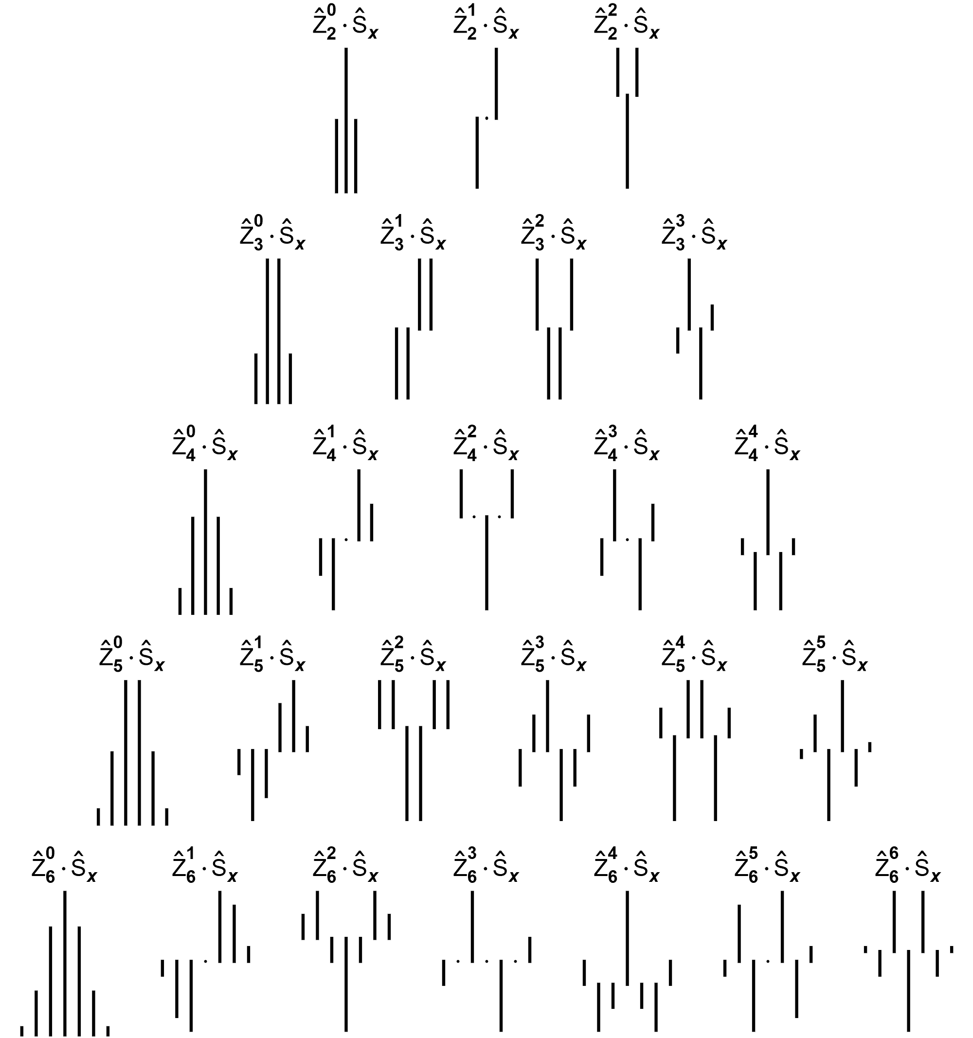
Figure 10: The quantum Pascal pyramid visualized as a triangle of the spectra of $\hat{Z}_{N}^{q}$ associated multiplets. The spectra have been scaled for equal visual visibility - the reader should be mindful of the actual scaling factors $2^{-N}\binom{N}{q}$.

IV Generalized quantum Pascal triangles

The familiar Pascal’s triangle (Table 1), which we may call $\mathbb{T}^{(0)}$, can be generalized to a triangle $\mathbb{T}^{(q)}$ that describes $\hat{z}_{N}^{q}$-associated multiplets.

Begin by considering the properties of $\mathbb{T}^{(0)}$, which occurs in the series expansion of $(1+x)^{N}$:

$$\sum_{k=0}^{N}a_{k}^{(0)}x^{k}=(1+x)^{N}$$ (16)

The coefficients $a_{k}^{(0)}$ are given by the familiar binomial coefficients:

$$a_{k}^{(0)}=\binom{N}{k}$$ (17)

	$m_{J}$	…	-$\frac{5}{2}$		-2		-$\frac{3}{2}$		-1		-$\frac{1}{2}$		0		+$\frac{1}{2}$		+1		+$\frac{3}{2}$		+2		+$\frac{5}{2}$		…
$N$
1											1				1
2									1				2				1
3							1				3				3				1
4					1				4				6				4				1
5			1				5				10				10				5				1
⋮

Table 1: $\mathbb{T}^{0}$, the triangle of binomial coefficients, describing the multiplet intensities of the operator $\hat{z}_{N}^{0}\hat{S}_{x}$.

The $\mathbb{T}^{(q)}$ triangles have a closely related generating function:

$$\sum_{k=0}^{N}a_{k}^{(q)}x^{k}=(1+x)^{N-q}(1-x)^{-q}$$ (18)

And an analytical expression for the coefficients of $a_{k}^{q}$ may be expressed in terms of Jacobi polynomials:

$$a_{k}^{(q)}=P_{N-k}^{(k-q,-N-1)}(3)$$ (19)

Some useful special cases are:

$$\begin{split}a_{k}^{(1)}&=\binom{N-1}{k-1}-\binom{N-1}{k}\\ &=\binom{N}{k}-2\binom{N-1}{k}\end{split}$$ (20)

$$a_{k}^{(2)}\ \ =\binom{N}{k}-4\binom{N-2}{k-1}$$ (21)

$$a_{k}^{(q)}=(-1)^{N+k}a_{k}^{(N-q)}$$ (22)

Several other potentially useful relations for $a_{k}^{(q)}$ may be found in the detailed mathematical analysis by Cação et al. [29], where they are called "a family of Pascal trapezoids".

We will also define:

$$A_{k}^{(q)}=\binom{N}{q}a_{k}^{(q)}$$ (23)

	$m_{J}$	…	-$\frac{5}{2}$		-2		-$\frac{3}{2}$		-1		-$\frac{1}{2}$		0		+$\frac{1}{2}$		+1		+$\frac{3}{2}$		+2		+$\frac{5}{2}$		…
$N$
1											-1				1
2									-1				0				1
3							-1				-1				1				1
4					-1				-2				0				2				1
5			-1				-3				-2				2				3				1
⋮

Table 2: $\mathbb{T}^{1}$, the triangle of the coefficients $a_{k}^{(1)}$, describing the multiplet intensities of the operator $\hat{z}_{N}^{1}S_{x}$.

	$m_{J}$	…	-$\frac{5}{2}$		-2		-$\frac{3}{2}$		-1		-$\frac{1}{2}$		0		+$\frac{1}{2}$		+1		+$\frac{3}{2}$		+2		+$\frac{5}{2}$		…
$N$
2									1				-2				1
3							1				-1				-1				1
4					1				0				-2				0				1
5			1				1				-2				-2				1				1
⋮

Table 3: $\mathbb{T}^{2}$, the triangle of the coefficients $a_{k}^{(2)}$, describing the multiplet intensities of the operator $\hat{z}_{N}^{2}S_{x}$.

	$m_{J}$	…	-3		-$\frac{5}{2}$		-2		-$\frac{3}{2}$		-1		-$\frac{1}{2}$		0		+$\frac{1}{2}$		+1		+$\frac{3}{2}$		+2		+$\frac{5}{2}$		+3		…
$N$
3									-1				3				-3				1
4							-1				2				0				-2				1
5					-1				1				2				-2				-1				1
6			-1				0				3				0				-3				0				1
⋮

Table 4: $\mathbb{T}^{3}$, the triangle of the coefficients $a_{k}^{(3)}$, describing the multiplet intensities of the operator $\hat{z}_{N}^{3}S_{x}$.

V Generalization of the de Moivre-Laplace theorem

The de Moivre-Laplace theorem is the famous, extraordinary mathematical result that a binomial distribution with $N$ elements converges to a Gaussian distribution as $N$ tends to infinity.
That is to say, a Gaussian distribution may be used to approximate a binomial distribution. In magnetic resonance terms, we could say that the familiar $\hat{Z}_{N}^{0}$-associated multiplet, for an $I_{N}S$ spin system, has a Fourier-transformed spectrum $S_{N}^{(0)}$ that is roughly traced by the Gaussian distribution $G_{N}^{(0)}$ (see Figure 11):

$$G_{N}^{(0)}\left(\nu\right)=\left(\frac{2}{\pi w}\right)\sqrt{\frac{2}{\pi N}}\exp{\left(-\frac{2}{N}\left(\frac{\nu}{J_{IS}}\right)^{2}\right)}$$ (24)

In which $\nu$ is the spectral frequency and $w$ is the spectral linewidth; the $2/\left(\pi w\right)$ factor arises under the assumption that the spectrum $S_{N}^{(0)}$ consists of a normalized sum of $A_{k}^{q}$-weighted individual Lorentzians $L\left(\nu\right)$:

$$S_{N}^{(0)}\left(\nu\right)=2^{-N}{\sum}_{m=-N/2}^{+N/2}A_{N/2+m}^{(0)}L\left(\nu\right)$$ (25)

Where each Lorentzian is characterized by a centre frequency $\nu_{0}=mJ_{IS}$ at which the maximum intensity is $2/\left(\pi w\right)$:

$$L\left(\nu\right)=\left(\frac{1}{\pi}\right)\frac{\left(w/2\right)}{\left(\nu-mJ_{IS}\right)^{2}+\left(w/2\right)^{2}}$$ (26)

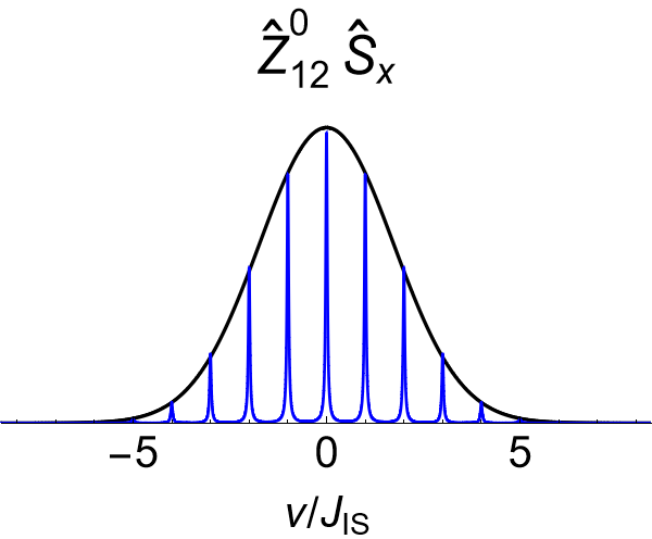
Figure 11: The spectrum $S_{12}^{(0)}$ (blue) of the $\hat{Z}_{12}^{0}$-associated multiplet and its Gaussian approximation $G_{12}^{(0)}$ (black). A linewidth of $w=0.05J_{IS}$ is assumed.

Now, consider the general case of $\hat{Z}_{N}^{q}$-associated multiplets, whose spectra may be denoted $S_{N}^{(q)}\left(\nu\right)$:

$$S_{N}^{(q)}\left(\nu\right)=2^{-N}{\sum}_{m=-N/2}^{+N/2}A_{N/2+m}^{(q)}L\left(\nu\right)$$ (27)

Remarkably, the result of Equation 24 can be generalized to $Z_{N}^{q}$-associated multiplets, which closely correspond to distributions given by the $q$-th Gaussian derivatives $G_{N}^{(q)}\left(\nu\right)$:

$$G_{N}^{(q)}\left(\nu\right)=\frac{(-1)^{q}\left(N/2\right)^{q}}{q!}\frac{d^{q}}{d\nu^{q}}G_{N}^{(0)}\left(\nu\right)$$ (28)

And, again exploiting the Rodrigues formula, $G_{N}^{(q)}$ may be expressed in terms of the well-known Hermite polynomials $H_{q}(x)$:

$$G_{N}^{(q)}\left(\nu\right)=\frac{\left(N/2\right)^{q/2}}{q!}H_{q}\left(\sqrt{\frac{2}{N}}\nu\right)G_{N}^{(0)}\left(\nu\right)$$ (29)

The reader is encouraged to compare the form of Equation 29 (see Figure 12) with the textbook case of the wavefunctions of the quantum harmonic oscillator, and the classical limit of Hermite-Gaussian laser modes [2, 3, 4, 6, 5, 7].

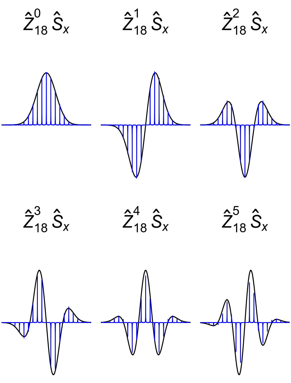
Figure 12: The spectra $S_{18}^{(q)}(\nu)$ (blue) of $\hat{Z}_{18}^{q}$-associated multiplets and the Hermite-Gaussian approximations $\hat{G}_{18}^{q}(\nu)$ (black). A line width of $w=0.02J_{IS}$ is assumed.

Derivatives are a measure of a rate of change, and - apart from the trivial relationship that $\hat{Z}_{N}^{q}$-associated multiplets change sign exactly $q$ times - there are at least two physical pictures associated with $\hat{Z}_{N}^{q}$ operators:

1. Each $\hat{Z}_{N}^{q}$ operator transforms with $\cos^{q}\left(\beta\right)$ under a rotation of flip angle $\beta$ in the $xy$-plane, defined through a rotation operator $\hat{R}_{\varphi}\left(\beta\right)=\exp\left[-i\beta\left(\cos(\varphi)\hat{I}_{x}+\sin(\varphi)\hat{I}_{y}\right)\right]$:

   $$\left\langle\hat{R}_{\varphi}\left(\beta\right)\hat{Z}_{N}^{q}\hat{R}_{\varphi}\left(-\beta\right)\rightarrow\hat{Z}_{N}^{q}\right\rangle=\frac{\left(\hat{R}_{\varphi}\left(\beta\right)\hat{Z}_{N}^{q}\hat{R}_{\varphi}\left(-\beta\right)|\hat{Z}_{N}^{q}\right)}{\left(\hat{Z}_{N}^{q}|\hat{Z}_{N}^{q}\right)}=\cos^{q}\left(\beta\right)$$ (30)

   Here, $\left(\hat{A}|\hat{B}\right)=\operatorname{Tr}\left[\hat{A}^{\dagger}\hat{B}\right]$ denotes the commonly used Liouville bracket, with curious readers referred to Pileio’s excellent book [30].

2. Each pure $\hat{Z}_{N}^{q}$ operator can be converted - with a $R_{\varphi}\left(\pi/2\right)$ rotation that may be realized by a simple $(90^{\circ})_{0}$ pulse - into $I$-spin multiple quantum coherence containing a mixture of coherence orders $p\in\left\{-q,-q+2\dots+q-2,+q\right\}$. If we use $\hat{\mathscr{Q}}_{q,p}$ to denote a $\hat{Z}_{N}^{q}$-derived operator of pure coherence order $p$, the following decomposition applies:

   $$\hat{R}_{\varphi}\left(\pi/2\right)\hat{Z}_{N}^{q}\hat{R}_{\varphi}\left(-\pi/2\right)=2^{-q}{{\sum}}_{\begin{subarray}{c}p=-q\\ q+p\in 2\mathbb{Z}\end{subarray}}^{+q}\binom{q}{\frac{1}{2}(q-p)}\hat{\mathscr{Q}}_{q,p}$$ (31)

   The maximum (absolute) coherence order available is $\lvert\pm q\rvert$, and by definition [31], $q$-quantum coherences transform with $\exp\left[-iq\times\beta\right]$ under a $z$-rotation of flip angle $\beta$, defined through the rotation operator $\hat{R}_{z}\left(\beta\right)=\exp\left[-i\beta\hat{I}_{z}\right]$:

   $$\left\langle\hat{R}_{z}\left(\beta\right)\hat{\mathscr{Q}}_{q,p}\hat{R}_{z}\left(-\beta\right)\rightarrow\hat{\mathscr{Q}}_{q,p}\right\rangle=\exp\left[-iq\times\beta\right]$$ (32)

   Here, it should be noted that common NMR strategies for the excitation of $n$-quantum coherences in $I_{n}S$ systems often involve the generation of $Z_{N}^{n}$-associated spin order in the preparation and/or readout steps [32].

VI Application: Bounds on Polarization Transfer

The problem of bounds on spin order transfer in magnetic resonance - a subset of the more general question of reachability in unitarily controlled Markovian quantum systems [33] - has been explored repeatedly [34, 35, 36, 37, 38, 39, 40, 41, 42, 43, 44, 45, 46, 47] in the field of NMR since the seminal set of papers by Sørensen [17, 48, 49]. At the more abstract level, this topic has also been shown to be intimately related to the mathematics of $C$-numerical ranges [50, 51, 52, 53].

Consider the following question: in an $I_{N}S$ spin system, what are the symmetry-constrained upper bounds on transfer of spin order from $\hat{I}_{z}$ to $\hat{S}_{z}$?

It is possible to answer this question and derive the bounds on $\hat{I}_{z}\rightarrow\hat{S}_{z}$ polarization transfer by using the quantum Pascal pyramid and the original Sørensen arguments [17].

The first step of a polarization transfer experiment is typically the conversion of $I$-spin order to an intermediate of maximally $I$-correlated $S$-spin order, which is trivial to do in this particular case with a unitary transformation corresponding to the aforementioned INEPT pulse sequence [20]:

$$\hat{I}_{z}\ \ \xrightarrow{90_{y}^{I}}\ \ \xrightarrow[t=1/(2J_{IS})]{H_{J}}\ \ \xrightarrow{90_{x}^{I}}\ \ 2\hat{I}_{z}\hat{S}_{z}$$ (33)

Recalling that:

$$2\hat{I}_{z}\hat{S}_{z}=\hat{Z}_{N}^{1}\hat{S}_{z}$$ (34)

And having obtained the expressions for the (eigenvalue) spectrum $\lambda(\hat{A})$ of the relevant operators:

$$\lambda\left(\hat{Z}_{N}^{0}\right)\in\left\{A_{0}^{(0)}\dots A_{N}^{(0)}\right\}=\left\{1,N\dots N,1\right\}$$ (35)

$$\lambda\left(\hat{Z}_{N}^{1}\right)\in\times\left\{A_{0}^{(1)}\dots A_{N}^{(1)}\right\}=\left\{-N,N(2-N)\dots N(N-2),N\right\}$$ (36)

We can calculate the trace (i.e. the sum of eigenvalues) of these operators:

$$\operatorname{Tr}\left(\hat{Z}_{N}^{0}\right)=\sum_{k=0}^{N}A_{k}^{(0)}=2^{N}$$ (37)

$$\operatorname{Tr}\left(\hat{Z}_{N}^{1}\right)=\sum_{k=0}^{N}A_{k}^{(1)}=0$$ (38)

As is obvious from its antisymmetric form, $\hat{Z}_{N}^{1}$ is traceless. In magnetic resonance terms, one would say that $I$-spin decoupling (which collapses the multiplet) leads to no detectable $\hat{Z}_{N}^{1}S_{x}$ signal, since the individual multiplet peak amplitudes, given by $\lambda\left(\hat{Z}_{N}^{1}\right)$, obviously add up to zero.

Nevertheless, we may appreciate that while unitary transformations cannot create or destroy spin order, they can certainly rearrange it. Suppose that one subjected $\hat{Z}_{N}^{1}$ to an ideal refocusing transformation (which can take, for example, the form of selective pulses [54] or pulsed analogues thereof [55, 17]) such that it was converted to an analogous operator $\left|\hat{Z}_{N}^{1}\right|$ with strictly positive eigenvalues:

$$\lambda\left(\left|\hat{Z}_{N}^{1}\right|\right)\in\left\{\left|A_{0}^{(1)}\right|\dots\left|A_{N}^{(1)}\right|\right\}=\left\{N,N(N-2)\dots N(N-2),N\right\}$$ (39)

The trace of this operator has a simple closed-form expression:

$$\operatorname{Tr}\left(\left|\hat{Z}_{N}^{1}\right|\right)=\sum_{k=0}^{N}\left|A_{k}^{(1)}\right|=2N\binom{N-1}{\left\lfloor N/2\right\rfloor}$$ (40)

The magnitude of the total detected signal, $s(\hat{A}.\hat{S}_{x})$, for a given $I$-spin longitudinal operator $\hat{A}$, is proportional to the gyromagnetic ratio of the "source" nucleus (from which spin order originates), and the trace of $\hat{A}$.
By evaluating the nominal, "unenhanced" signal, of $S_{x}$:

$$s\left(\hat{Z}_{N}^{0}\hat{S}_{x}\right)\propto\left|\gamma_{S}\right|\operatorname{Tr}\left(\hat{Z}_{N}^{0}\right)$$ (41)

And the maximally enhanced signal of refocused $I$-correlated spin order:

$$s\left(\left|\hat{Z}_{N}^{1}\right|\hat{S}_{x}\right)\propto\left|\gamma_{I}\right|\operatorname{Tr}\left(\left|\hat{Z}_{N}^{1}\right|\right)$$ (42)

We may obtain the maximum possible enhancement factor in terms of $k_{\gamma}=\left|\gamma_{I}/\gamma_{S}\right|$:

$$\begin{split}b_{\rm{max}}\left(\hat{I}_{z}\rightarrow\hat{S}_{z}\right)&=\frac{s\left(\left|\hat{Z}_{N}^{1}\right|\hat{S}_{x}\right)}{s\left(\hat{Z}_{N}^{0}\hat{S}_{x}\right)}\\ &=k_{\gamma}\frac{\operatorname{Tr}\left(\left|\hat{Z}_{N}^{1}\right|\right)}{\operatorname{Tr}\left(\hat{Z}_{N}^{0}\right)}\\ &=k_{\gamma}2^{1-N}N\binom{N-1}{\lfloor{N/2}\rfloor}\end{split}$$ (43)

Which is a form of Sørensen’s original expression [17], and can be expressed in other elegant forms that have not previously appeared in the NMR literature:

$$\begin{split}&=k_{\gamma}\times\begin{cases}\frac{N\text{!!}}{(N-1)\text{!!}}&\rm{for}\leavevmode\nobreak\ N\in 2\mathbb{Z}+1\\ \frac{(N-1)\text{!!}}{(N-2)\text{!!}}&\rm{for}\leavevmode\nobreak\ N\in 2\mathbb{Z}\end{cases}\\ &=2k_{\gamma}\times MD_{N}\end{split}$$ (44)

Here, $!!$ denotes the double factorial while $MD_{N}$ is the mean absolute deviation of a symmetric binomial distribution with $N$ elements, as first discovered by de Moivre in the 1730 work Miscellanea Analytica, a story discussed in detail by Diaconis and Zabell [56].

In a strange accident of history, it was de Moivre’s fateful encounter with the latter $MD_{N}$ problem that led him to an early form of the central limit theorem (first appearing in The Doctrine of Chances in 1738) a result so far ahead of its time that it was only rediscovered almost a century later by Laplace, the basis of the modern nomenclature "de Moivre-Laplace theorem". Towards the end of the last century, generalizations of this result were exploited by mathematicians [56] to prove various relationships involving - among other aspects - the Jacobi and Hermite polynomials that appear in this paper. It may be concluded that in the search for deeper patterns within quantum angular momentum, we must have done little more than retraced de Moivre’s old steps, perhaps with an element of time reversal.

References

- [1] Brian E. Mann “The Analysis of First-Order Coupling Patterns in NMR Spectra” In Journal of Chemical Education 72.7 American Chemical Society, 1995, pp. 614 DOI: 10.1021/ed072p614
- [2] L. Allen, M.. Beijersbergen, R… Spreeuw and J.. Woerdman “Orbital Angular Momentum of Light and the Transformation of Laguerre-Gaussian Laser Modes” In Physical Review A 45.11 American Physical Society, 1992, pp. 8185–8189 DOI: 10.1103/PhysRevA.45.8185
- [3] G. Nienhuis and L. Allen “Paraxial Wave Optics and Harmonic Oscillators” In Physical Review A 48.1 American Physical Society, 1993, pp. 656–665 DOI: 10.1103/PhysRevA.48.656
- [4] S.. Steely “Harmonic Oscillator Fiducials for Hermite-Gaussian Laser Beams” In Optics and Lasers in Engineering 28.3, 1997, pp. 213–228 DOI: 10.1016/S0143-8166(97)00003-1
- [5] Jörg Enderlein and Francesco Pampaloni “Unified Operator Approach for Deriving Hermite–Gaussian and Laguerre–Gaussian Laser Modes” In JOSA A 21.8 Optica Publishing Group, 2004, pp. 1553–1558 DOI: 10.1364/JOSAA.21.001553
- [6] Ole Steuernagel “Equivalence between Focused Paraxial Beams and the Quantum Harmonic Oscillator” In American Journal of Physics 73.7, 2005, pp. 625–629 DOI: 10.1119/1.1900099
- [7] John S. Briggs “The Propagation of Hermite–Gauss Wave Packets in Optics and Quantum Mechanics” In Natural Sciences 4.1, 2024, pp. e20230012 DOI: 10.1002/ntls.20230012
- [8] Fabrizio Colombo, Elodie Pozzi, Irene Sabadini and Brett Wick “Evolution of Superoscillations for Spinning Particles” In Proceedings of the American Mathematical Society, Series B 10.11, 2023, pp. 129–143 DOI: 10.1090/bproc/159
- [9] Yakir Aharonov, David Z. Albert and Lev Vaidman “How the Result of a Measurement of a Component of the Spin of a Spin-1/2 Particle Can Turn out to Be 100” In Physical Review Letters 60.14 American Physical Society, 1988, pp. 1351–1354 DOI: 10.1103/PhysRevLett.60.1351
- [10] M.. Berry and S. Popescu “Evolution of Quantum Superoscillations and Optical Superresolution without Evanescent Waves” In Journal of Physics A: Mathematical and General 39.22, 2006, pp. 6965 DOI: 10.1088/0305-4470/39/22/011
- [11] Michael Berry et al. “Roadmap on Superoscillations” In Journal of Optics 21.5 IOP Publishing, 2019, pp. 053002 DOI: 10.1088/2040-8986/ab0191
- [12] Yakir Aharonov, Jussi Behrndt, Fabrizio Colombo and Peter Schlosser “A Unified Approach to Schrödinger Evolution of Superoscillations and Supershifts” In Journal of Evolution Equations 22.1, 2022, pp. 26 DOI: 10.1007/s00028-022-00770-1
- [13] Nicolas D. Werbeck and D. Hansen “Heteronuclear Transverse and Longitudinal Relaxation in AX4 Spin Systems: Application to 15N Relaxations in 15NH4+” In Journal of Magnetic Resonance 246, 2014, pp. 136–148 DOI: 10.1016/j.jmr.2014.06.010
- [14] D. Hansen “Measurement of 15N Longitudinal Relaxation Rates in 15NH4+ Spin Systems to Characterise Rotational Correlation Times and Chemical Exchange” In Journal of Magnetic Resonance 279, 2017, pp. 91–98 DOI: 10.1016/j.jmr.2017.01.015
- [15] Brennan J. Walder and Keith J. Fritzsching “Weighted AnX Multiplets” In Journal of Magnetic Resonance 347, 2023, pp. 107353 DOI: 10.1016/j.jmr.2022.107353
- [16] O.W. Sørensen et al. “Product Operator Formalism for the Description of NMR Pulse Experiments” In Progress in Nuclear Magnetic Resonance Spectroscopy 16, 1984, pp. 163–192 DOI: 10.1016/0079-6565(84)80005-9
- [17] Ole Winneche Sørensen “Polarization Transfer Experiments in High-Resolution NMR Spectroscopy” In Progress in Nuclear Magnetic Resonance Spectroscopy 21.6, 1989, pp. 503–569 DOI: 10.1016/0079-6565(89)80006-8
- [18] A. Wünsche “The Role of Jacobi Polynomials in the Theory of Hermite and Laguerre 2D Polynomials” In Journal of Computational and Applied Mathematics 153.1, Proceedings of the 6th International Symposium on Orthogonal Poly Nomials, Special Functions and Their Applications, Rome, Italy, 18-22 June 2001, 2003, pp. 521–529 DOI: 10.1016/S0377-0427(02)00632-5
- [19] E.. Abramochkin and V.. Volostnikov “Generalized Gaussian Beams” In Journal of Optics A: Pure and Applied Optics 6.5, 2004, pp. S157 DOI: 10.1088/1464-4258/6/5/001
- [20] Gareth A. Morris and Ray Freeman “Enhancement of Nuclear Magnetic Resonance Signals by Polarization Transfer” In Journal of the American Chemical Society 101.3 American Chemical Society, 1979, pp. 760–762 DOI: 10.1021/ja00497a058
- [21] David M. Doddrell, David T. Pegg, William Brooks and M. Bendall “Enhancement of Silicon-29 or Tin-119 NMR Signals in the Compounds M(CH3)(n)Cl(4-n) M = Silicon or Tin, n = 4, 3, 2) Using Proton Polarization Transfer. Dependence of the Enhancement on the Number of Scalar Coupled Protons” In Journal of the American Chemical Society 103.3 American Chemical Society, 1981, pp. 727–728 DOI: 10.1021/ja00393a067
- [22] David T Pegg, David M Doddrell, William M Brooks and M Robin Bendall “Proton Polarization Transfer Enhancement for a Nucleus with Arbitrary Spin Quantum Number from n Scalar Coupled Protons for Arbitrary Preparation Times” In Journal of Magnetic Resonance (1969) 44.1, 1981, pp. 32–40 DOI: 10.1016/0022-2364(81)90186-4
- [23] Klaus G.. Pachler and Philippus L. Wessels “Intensity Gains with a Progressive Saturation SPI n.m.r. Experiment. The Degenerate A—X3 Case” In Organic Magnetic Resonance 9.9, 1977, pp. 557–558 DOI: 10.1002/mrc.1270090915
- [24] Martin Erik Horn “The Didactical Relevance of the Pauli Pascal Triangle (Die Didaktische Relevanz Des Pauli-Pascal-Dreiecks)”, 2006 DOI: 10.48550/arXiv.physics/0611277
- [25] Martin Erik Horn “Pauli Pascal Pyramids, Pauli Fibonacci Numbers, and Pauli Jacobsthal Numbers”, 2007 DOI: 10.48550/arXiv.0711.4030
- [26] Mohamed Sabba “Catalan Triangle and Clebsch-Gordan Multiplicities – Sabba’s NMR Blog”, 2024 URL: https://sabba.me/nmr/2024/02/20/catalan-triangle-and-clebsch-gordan-multiplicities/
- [27] “Chapter 13: The Symmetric Group” In Group Theory and Its Application to the Quantum Mechanics of Atomic Spectra 5, Group Theory Elsevier, 1959, pp. 124–141 DOI: 10.1016/B978-0-12-750550-3.50018-5
- [28] H.. Forder “Some Problems in Combinatorics” In The Mathematical Gazette 45.353, 1961, pp. 199–201 DOI: 10.2307/3612775
- [29] Isabel Cacao, Helmuth R Malonek, M Irene Falcao and Graca Tomaz “Combinatorial Identities Associated with a Multidimensional Polynomial Sequence” In Journal of Integer Sequences 21, 2018 URL: https://cs.uwaterloo.ca/journals/JIS/VOL21/Falcao/falcao2.html
- [30] Giuseppe Pileio “Lectures On Spin Dynamics: The Theoretical Minimum” The Royal Society of Chemistry, 2022 DOI: 10.1039/9781837670871
- [31] Geoffrey Bodenhausen, Herbert Kogler and R.R. Ernst “Selection of Coherence-Transfer Pathways in NMR Pulse Experiments” In Journal of Magnetic Resonance (1969) 58.3, 1984, pp. 370–388 DOI: 10.1016/0022-2364(84)90142-2
- [32] Rui Huang et al. “An Enhanced Sensitivity Methyl 1H Triple-Quantum Pulse Scheme for Measuring Diffusion Constants of Macromolecules” In Journal of Biomolecular NMR 68.4, 2017, pp. 249–255 DOI: 10.1007/s10858-017-0122-9
- [33] Frederik Ende “Reachability in Controlled Markovian Quantum Systems: An Operator-Theoretic Approach”, 2020, pp. 264 DOI: 10.14459/2020md1559809
- [34] Malcolm H Levitt “Unitary Evolution, Liouville Space, and Local Spin Thermodynamics” In Journal of Magnetic Resonance (1969) 99.1, 1992, pp. 1–17 DOI: 10.1016/0022-2364(92)90151-V
- [35] A.G Redfield “On the Upper Bound of Spin Polarization Transfer” In Journal of Magnetic Resonance (1969) 92.3, 1991, pp. 642–644 DOI: 10.1016/0022-2364(91)90363-X
- [36] Niels Chr Nielsen and Ole W Sørensen “2D Bounds on Polarization Transfer Involving Quadrupolar Spin Nuclei” In Journal of Magnetic Resonance (1969) 99.1, 1992, pp. 214–222 DOI: 10.1016/0022-2364(92)90171-3
- [37] J. Stoustrup et al. “Generalized Bound on Quantum Dynamics: Efficiency of Unitary Transformations between Non-Hermitian States” In Physical Review Letters 74.15 American Physical Society, 1995, pp. 2921–2924 DOI: 10.1103/PhysRevLett.74.2921
- [38] Niels Chr Nielsen and Ole W Sørensen “Accessible States in Liouville Space. A Two-Dimensional Extension of the Universal Bound on Spin Dynamics Applied to Polarization Transfer in INSM Spin-12 Systems” In Journal of Magnetic Resonance (1969) 99.3, 1992, pp. 449–465 DOI: 10.1016/0022-2364(92)90202-I
- [39] Shanmin Zhang, Ping Xu, Ole W. Sørensen and Richard R. Ernst “Absence of Conservation Laws and the Reciprocity Relation in Polarization-Transfer Experiments” In Concepts in Magnetic Resonance 6.4, 1994, pp. 275–292 DOI: 10.1002/cmr.1820060403
- [40] N.C. Nielsen and O.W. Sorensen “Conditional Bounds on Polarization Transfer” In Journal of Magnetic Resonance, Series A 114.1, 1995, pp. 24–31 DOI: 10.1006/jmra.1995.1101
- [41] S.. Glaser et al. “Unitary Control in Quantum Ensembles: Maximizing Signal Intensity in Coherent Spectroscopy” In Science 280.5362 American Association for the Advancement of Science, 1998, pp. 421–424 DOI: 10.1126/science.280.5362.421
- [42] T. Untidt et al. “Design of NMR Pulse Experiments with Optimum Sensitivity: Coherence-Order-Selective Transfer in I2S and I3S Spin Systems” In Molecular Physics 95.5, 1998, pp. 787–796 DOI: 10.1080/002689798166413
- [43] Thomas S. Untidt and Niels Chr. Nielsen “Analytical Unitary Bounds on Quantum Dynamics: Design of Optimum NMR Experiments in Two-Spin-12 Systems” In The Journal of Chemical Physics 113.19, 2000, pp. 8464–8471 DOI: 10.1063/1.1318756
- [44] Malcolm H. Levitt “Symmetry Constraints on Spin Dynamics: Application to Hyperpolarized NMR” In Journal of Magnetic Resonance 262, 2016, pp. 91–99 DOI: 10.1016/j.jmr.2015.08.021
- [45] Andrey N. Pravdivtsev, Danila A. Barskiy, Jan-Bernd Hövener and Igor V. Koptyug “Symmetry Constraints on Spin Order Transfer in Parahydrogen-Induced Polarization (PHIP)” In Symmetry 14.3 Multidisciplinary Digital Publishing Institute, 2022, pp. 530 DOI: 10.3390/sym14030530
- [46] M.. Levitt and C. Bengs “Hyperpolarization and the Physical Boundary of Liouville Space” In Magnetic Resonance 2.1, 2021, pp. 395–407 DOI: 10.5194/mr-2-395-2021
- [47] Christian Bengs “Hyperpolarisation Criteria in Magnetic Resonance” In Journal of Magnetic Resonance 360, 2024, pp. 107631 DOI: 10.1016/j.jmr.2024.107631
- [48] Ole W Sørensen “A Universal Bound on Spin Dynamics” In Journal of Magnetic Resonance (1969) 86.2, 1990, pp. 435–440 DOI: 10.1016/0022-2364(90)90278-H
- [49] Ole W Sørensen “The Entropy Bound as a Limiting Case of the Universal Bound on Spin Dynamics. Polarization Transfer in INSM Spin Systems” In Journal of Magnetic Resonance (1969) 93.3, 1991, pp. 648–652 DOI: 10.1016/0022-2364(91)90095-B
- [50] Chi-Kwong Li, Tin-Yau Tam and Nam-Kiu Tsing “The Generalized Spectral Radius, Numerical Radius and Spectral Norm” In Linear and Multilinear Algebra 16.1-4 Taylor & Francis, 1984, pp. 215–237 DOI: 10.1080/03081088408817624
- [51] Chi-Kwong Li “C-Numerical Ranges and C-numerical Radii” In Linear and Multilinear Algebra Gordon and Breach Science Publishers, 1994 DOI: 10.1080/03081089408818312
- [52] Thomas Schulte-Herbrüggen, Gunther Dirr, Uwe Helmke and Steffen J. Glaser “The Significance of the C -Numerical Range and the Local C -Numerical Range in Quantum Control and Quantum Information” In Linear and Multilinear Algebra 56.1-2 Taylor & Francis, 2008, pp. 3–26 DOI: 10.1080/03081080701544114
- [53] G. Dirr, U. Helmke, M. Kleinsteuber and Th. Schulte-Herbrüggen “Relative C -Numerical Ranges for Applications in Quantum Control and Quantum Information” In Linear and Multilinear Algebra 56.1-2 Taylor & Francis, 2008, pp. 27–51 DOI: 10.1080/03081080701535898
- [54] Soumya Singha Roy et al. “Enhancement of Quantum Rotor NMR Signals by Frequency-Selective Pulses” In Journal of Magnetic Resonance 250, 2015, pp. 25–28 DOI: 10.1016/j.jmr.2014.11.004
- [55] Niels Chr Nielsen, Henrik Bildsøe, Hans J Jakobsen and Ole W Sørensen “Composite Refocusing Sequences and Their Application for Sensitivity Enhancement and Multiphcity Filtration in INEPT and 2D Correlation Spectroscopy” In Journal of Magnetic Resonance (1969) 85.2, 1989, pp. 359–380 DOI: 10.1016/0022-2364(89)90149-2
- [56] Persi Diaconis and Sandy Zabell “Closed Form Summation for Classical Distributions: Variations on a Theme of De Moivre” In Statistical Science 6.3 Institute of Mathematical Statistics, 1991, pp. 284–302 JSTOR: http://www.jstor.org/stable/2245429