Bringing memory to Boolean networks: a unifying framework

Abstract. Boolean networks are extensively applied as models of complex dynamical systems, aiming at capturing essential features related to causality and synchronicity of the state changes of components along time. Dynamics of Boolean networks result from the application of their Boolean map according to a so-called update mode, specifying the possible transitions between network configurations. In this paper, we explore update modes that possess a memory on past configurations, and provide a generic framework to define them. We show that recently introduced modes such as the most permissive and interval modes can be naturally expressed in this framework. We propose novel update modes, the history-based and trapping modes, and provide a comprehensive comparison between them. Furthermore, we show that trapping dynamics, which further generalize the most permissive mode, correspond to a rich class of networks related to transitive dynamics and encompassing commutative networks. Finally, we provide a thorough characterization of the structure of minimal and principal trapspaces, bringing a combinatorial and algebraic understanding of these objects.

1 Introduction

Boolean networks (BNs) are a fundamental framework for addressing complex systems, with prominent applications in biology, ecology, and social sciences [12, 18, 8, 17, 10]. Closely related to cellular automata, BNs consider a finite number of components, or automata, each having its own neighborhood and rule for computing its next Boolean state from the configuration of the network.

A large amount of theoretical work underlined the importance of the scheduling of the update of states of components for the dynamics that can be generated, the so-called update mode. One natural mode is the parallel (or synchronous) mode, where all components are updated simultaneously and instantaneously, generating deterministic dynamics. Another classical update mode is the (general) asynchronous mode: any subset of components can be updated simultaneously, potentially leading to non-deterministic dynamics. Any trajectory, i.e., succession of configurations, computed with the parallel mode can also be computed using the asynchronous mode. The converse is, in general, false. Update modes also impact the so-called limit configurations, that are the configurations from which any reachable configuration can return to them. Limit configurations constitute the attractors of dynamics and are a prime subject of study in the literature, including their robustness to update modes [2, 1].

When employing BNs as models of complex dynamical systems, such as gene regulation within cells, update modes aim at reflecting hypotheses related to the duration, speed, probability, and other quantitative features of the transitions. For instance, asynchronous modes can be motivated by the fact that genes can require different amounts of proteins to become active.

There is a rich catalog of update modes defined in the literature that consider various restrictions related to the synchronicity and sequentiality of updates. These modes can be compared in terms of weak simulation relations: an update mode $\mu$ weakly simulates another update mode $\mu^{\prime}$ if, for any BN, for any pair of its configurations, if there is a trajectory between these configurations with $\mu^{\prime}$, then there is a trajectory with $\mu$ as well. This relationship enables to draw a hierarchy of update modes [16], where most of them are weakly simulated by the general asynchronous mode. There is a notable exception with a couple of recently introduced unconventional update modes that enable generating trajectories impossible with the general asynchronous mode. The interval update mode [5], inspired by work on concurrent systems by the means of Petri nets, considers cases when the state change of a component can be put on hold for a while. During that period, other components still observe the old value of it, and can evolve accordingly and before the new state is finally revealed. This can generate new trajectories, leading to configurations that are not reachable with the general asynchronous mode. The most permissive update mode [14] generalizes this abstraction by considering that a component in the process of changing of state can be viewed as in superposition of both states. This mode was motivated by the Boolean modeling of quantitative systems: e.g., during the increase of the state of a component, there can be a time when it is sufficiently high for acting on one component and not high enough for acting on another one. Lately, the cuttable extension update mode [13] was introduced as a mode generating more trajectories than the interval, but less than the most permissive, in order to better capture monotone changes of component states.

One of the common ingredients between the interval, cuttable, and most permissive modes is the account of some kind of memory of the state changes: it is because they remember that a component is changing that they can interleave additional transitions before applying the change, generating additional but plausible trajectories. Note that another mode named BNs with memory has been recently introduced [9]. However, as demonstrated in [15], it actually boils down to having a fixed set of components to update asynchronously while another set updates in parallel.

In this paper, we aim at emphasizing on the effect of memory in update modes of BNs, both by introducing new modes around this feature, and by studying their relationship with others, as well as related combinatorial properties.

We propose a unifying framework to define such update modes by characterizing the trajectories they generate. This allows to account for a sequence of configurations that have been computed since an initial one, and compute elongation of the trajectory based on this sequence. We notably introduce in Sect. 2 two elementary update modes using memory: the history-based update mode, where the next configuration is computed from the current one and one component has been updated according to any configuration in the past; and the trapping update mode, where the next configuration is computed from any configuration of the past, and one component has been updated according to any configuration in the past. Intuitively, the history-based mode extends the asynchronous by allowing to take any configuration of the past, instead of the latter only, to compute the next state of the component. Then, the trapping mode extends the history-based by allowing to take any configuration of the past as the base next configuration. This somehow allows for jumping back in time, while having the knowledge of the sequence of configurations before the jump.

One can naturally derive that the asynchronous trajectories are a subset of history-based trajectories, being themselves a subset of trapping trajectories. In this paper, we establish simulation and weak simulation relationships with the interval, cuttable, and most permissive update modes (Sect. 3). In particular, we demonstrate that cuttable and history-based modes are incomparable, while both weakly simulating the interval, and both being weakly simulated by the most permissive, which in turns, is weakly simulated by the trapping mode. We provide a similar hierarchy by considering inclusion of trajectories (simulation). We also show that the trapping mode is weakly bisimilar to a subcube-based update mode. The (smallest) subcube enclosing the configurations of the trajectory is the set of configurations that can be composed of any state of the components in the past. In the subcube-based mode, the trajectory can be extended with any of such configurations, where the state of one component has been updated according to any configuration of this subcube.

Another important result of Sect. 3 is that most permissive and trapping modes coincide on the reachability of configurations in minimal trapspaces. Thus, both dynamics have the same limit configurations, and the same limit configurations reachable from any configuration.

Finally, in Sect. 4, we further explore combinatorics of the trapping mode and show that trapping dynamics form a rich class of graphs. In particular, they correspond to general asynchronous dynamics being transitive, and encompass commutative networks. The principal trapspace of a configuration (for a given BN) is the smallest trapspace that contains that configuration. All trajectories in the update modes considered in this paper are bounded by the principal trapspace of their starting point; in fact, the trapping update mode can visit the entire principal trapspace. We then investigate the structure of principal trapspaces. Clearly, every subcube can be a principal trapspace, however the collection of all principal trapspaces of a BN is highly structured (we call it pre-principal in the sequel; see Lemma 4.13). Moreover, the collection of all trapspaces of a BN is also highly structured (roughly speaking, it is closed under union and intersection; see Lemma 4.14). In Theorem 4.9 we show that two BNs have the same trapspaces if and only if they have the same principal trapspaces. In other words, the collection of principal trapspaces of a BN completely characterises the collection of all its trapspaces. We then strengthen this result and show in Theorem 4.11 that there is a three-way equivalence between: BNs with transitive general asynchronous graphs (which we call trapping networks), collections of principal trapspaces of BNs, and collections of trapspaces of BNs. We finally consider minimal trapspaces, which form a subset of principal trapspaces. Unlike principal trapspaces, the collection of minimal trapspaces does not determine the collection of all trapspaces. However, we are able to characterise collections of minimal trapspaces of BNs and to obtain results analogous to Theorems 4.9 and 4.11.

The paper is structured as follows. Sect. 2 introduces a generic framework to express memory-based update modes which is employed to define novel trapping, history-based, and subcube-based update modes, and give equivalent definitions of asynchronous, most permissive, interval and cuttable update modes. Then, Sect. 3 provides a simulation and weak-simulation hierarchy between those updates. Focusing on trapping and most permissive update modes, Sect. 4 brings combinatorial characterization of trapping dynamics and of collections of trapspaces and minimal trapspaces. Finally, Sect. 5 discusses the contributions of the paper.

Notations

We denote the Boolean set by $\mathbb{B}=\{0,1\}$ and for any positive integer $n$, we denote $[n]=\{1,\dots,n\}$. A configuration is $x=(x_{1},\dots,x_{n})\in\mathbb{B}^{n}$. For any $S\subseteq[n]$, we denote $x_{S}=(x_{s}:s\in S)$ and we use the notation $x=(x_{S},x_{-S})$. We shall identify an element $i\in[n]$ with the corresponding singleton $\{i\}$, so that $x=(x_{i},x_{-i})$ for instance. For any two configurations $x,y\in\mathbb{B}^{n}$, we denote the set of positions where they differ by $\Delta(x,y)=\{i\in[n]:x_{i}\neq y_{i}\}$ and their Hamming distance by $d_{\mathrm{H}}(x,y)=|\Delta(x,y)|$.

A subcube of $\mathbb{B}^{n}$ is any $X\subseteq\mathbb{B}^{n}$ such that there exist two disjoint sets of positions $S,T\subseteq[n]$ with $X=\{x\in\mathbb{B}^{n}:x_{S}=0,x_{T}=1\}$. For any set $A\subseteq\mathbb{B}^{n}$, the principal subcube of $A$, denoted by $[A]$, is the smallest subcube containing $A$. If $A=\{a_{1},\dots,a_{k}\}$, we also denote $[A]=[a_{1},\dots,a_{k}]$. If $X$ is a subcube and $x\in X$, then there is a unique $y\in X$ such that $X=[x,y]$; we refer to $y$ as the opposite of $x$ in $X$, and we denote it by $y=X-x$. We denote the set of subcubes of $\mathbb{B}^{n}$ as $\mathrm{S}(n)$ and the set of all collections of subcubes of $\mathbb{B}^{n}$ as $\mathrm{A}(n)=2^{\mathrm{S}(n)}$.

A Boolean network (BN) of dimension $n$ is a mapping $f:\mathbb{B}^{n}\to\mathbb{B}^{n}$. We denote the set of BNs of dimension $n$ as $\mathrm{F}(n)$. Any BN $f\in\mathrm{F}(n)$ can be viewed as $f=(f_{1},\dots,f_{n})$ where $f_{i}(x)=f(x)_{i}$ for all $i\in[n]$. For any $S\subseteq[n]$ and any $f\in\mathrm{F}(n)$, the update of $S$ according to $f$ is represented by the BN $f^{(S)}\in\mathrm{F}(n)$ where

$$f^{(S)}(x)=(f_{S}(x),x_{-S}).$$

In particular, $f^{([n])}=f$ and $f^{(\emptyset)}=\mathrm{id}$. We note the distinction between the update $f^{(i)}$ (given by $f^{(i)}(x)=(f_{i}(x),x_{-i})$) and the power $f^{i}=f\circ f\circ\dots\circ f$ ($i$ terms). We can then compose those updates, so that if $S_{1},\dots,S_{k}\subseteq[n]$, we obtain

$$f^{(S_{1},\dots,S_{k})}=f^{(S_{k})}\circ f^{(S_{k-1})}\circ\dots\circ f^{(S_{1})}.$$

A trapspace of $f\in\mathrm{F}(n)$ is a subcube $X\subseteq\mathbb{B}^{n}$ such that $f(X)\subseteq X$. The collection of all trapspaces of $f$, denoted by $\mathcal{T}(f)$, is closed under intersection. Then for any $x\in\mathbb{B}^{n}$,there is a smallest trapspace of $f$ that contains $x$, which we shall refer to as the principal trapspace of $x$ (with respect to $f$). For the sake of simplicity, we denote it by $T_{f}(x)$. The principal trapspace $T_{f}(x)$ can be recursively computed as follows: let $T_{0}=\{x\}$ and $T_{i}=[T_{i-1}\cup f(T_{i-1})]$, then $T_{n}=T_{f}(x)$. In particular, $[x,f(x)]\subseteq T_{f}(x)$. The collection of all principal trapspaces of $f$ is denoted by $\mathcal{P}(f)$. A trapspace $T$ is minimal if there is no trapspace $T^{\prime}$ with $T^{\prime}\subset T$. Clearly, any minimal trapspace is principal, but the converse does not necessarily hold. The collection of minimal trapspaces of $f$ is denoted by $\mathcal{M}(f)$. Minimal trapspaces of BNs have been notably studied for their relation with limit (ultimately periodic) configurations: each minimal trapspace necessarily contains at least one limit configuration [11, 14].

A (directed) graph is $\Gamma=(V,E)$, where $V$ is the set of vertices and $E\subseteq V^{2}$ is the set of edges. A graph $\Gamma$ is reflexive if for all $v\in V$, $(v,v)\in E$; $\Gamma$ is symmetric if $(u,v)\in E$ implies $(v,u)\in E$ for all $u,v\in V$; and $\Gamma$ is transitive if $(u,v),(v,w)\in E$ implies $(u,w)\in E$ for all $u,v,w\in E$. The out-neighbourhood of a vertex $v$ is $N^{out}(\Gamma;v)=\{u\in V:(v,u)\in E\}$.

The asynchronous graph of a BN $f\in\mathrm{F}(n)$ is the graph $\mathtt{A}(f)=(V,E)$ where $V=\mathbb{B}^{n}$ and

$$E=\{(x,f^{(i)}(x)):x\in\mathbb{B}^{n},i\in[n]\}.$$

Note that in most literature, one removes the loops $(x,x)$ from the asynchronous graph, that occur every time $f_{i}(x)=x_{i}$, yet we shall keep those loops instead in our definition. However, when drawing the asynchronous graph, we shall not display the loops and instead draw the underlying hypercube with thin black lines and the arcs of the graph with thick blue arrows. See below for an example of a BN, for which we give the asynchronous graph and all the trapspaces.

Example 1.1.

Let $f\in\mathrm{F}(3)$ be defined as

$x$	$f(x)$
$000$	$110$
$001$	$100$
$010$	$000$
$011$	$110$
$100$	$100$
$101$	$101$
$110$	$110$
$111$	$110$

The asynchronous graph of $f$ is given by:

We then have $\mathcal{T}(f)=\{A,B,C,D,E,F,G,H\}$, $\mathcal{P}(f)=\{A,B,C,D,E,F\}$ and $\mathcal{M}(f)=\{D,E,F\}$ with

$$T_{f}(000)=T_{f}(010) = A =\{x:x_{3}=0\}$$

$$T_{f}(111) = B =\{x:x_{12}=11\}$$

$$T_{f}(011)=T_{f}(001) = C =\{x\}$$

$$T_{f}(110) = D =\{x:x_{12}=11,x_{3}=0\}$$

$$T_{f}(100) = E =\{x:x_{1}=1,x_{23}=00\}$$

$$T_{f}(101) = F =\{x:x_{13}=11,x_{2}=0\}$$

$$G =\{x:x_{1}=1,x_{3}=0\}$$

$$H =\{x:x_{1}=1\}.$$

2 Update modes for dynamics with memory

In this section, we give a unified framework for defining update modes that rely on memory along trajectories. We focus on the fully asynchronous case, whereby one component updates its state at each given time.

A (fully asynchronous) trajectory is a sequence $(x^{0},\dots,x^{l})\in(\mathbb{B}^{n})^{*}$ such that for all $1\leq a\leq l$, there exists $t\in[x^{0},\dots,x^{a-1}]$ such that $d_{\mathrm{H}}(t,x^{a})\leq 1$. A prefix of the trajectory $(x^{0},\dots,x^{l})$ is any $(x^{0},\dots,x^{a})$ for $0\leq a\leq l$, or the empty sequence. An update mode is a mapping $\mu$ which assigns, for any $n$ and any BN $f\in\mathrm{F}(n)$, a collection of trajectories closed by taking prefixes (i.e. if $(x^{0},\dots,x^{l})\in\mu(f)$, then $(x^{0},\dots,x^{a})\in\mu(f)$). Since we shall fix the BN in the remainder of this section, we shall omit the dependence on $f$ in our notation. To emphasize that $(x^{0},\dots,x^{l})$ is a trajectory according to $\mu$, we write $x^{0}\to_{\mu}\dots\to_{\mu}x^{l}$. A pair of configurations $(x,y)$ is a reachability pair for an update mode $\mu$ if there exists a trajectory $x=x^{0}\to_{\mu}\dots\to_{\mu}x^{l}=y$, and we say that $y$ is reachable from $x$.

We aim to model updates where there are delays in the propagation of the updated values. Any trajectory can be represented using the starting configuration $x^{0}$ and for all $1\leq a\leq l$, a triple

$$w^{a}=(i^{a},s^{a},t^{a})$$

so that the next configuration is

$$x^{a}=(f_{i^{a}}(s^{a}),t^{a}).$$

Here is the intuition behind this representation and the kind of restrictions we shall apply to the word $w^{a}$. The component $i^{a}$ updating its state at step $a$ does not necessarily apply its update function $f_{i^{a}}$ to the current configuration $x^{a-1}$ but to a configuration $s^{a}$ built up of states with different timestamps. More precisely, we have $s^{a}$ with $s^{a}_{j}=x_{j}^{b_{j}}$ for all $j$, i.e. $s^{a}\in[x^{0},\dots,x^{a-1}]$. In the following, we will also allow for the other components to choose any value that has already been observed in the trajectory; we obtain a target configuration $t^{a}\in[x^{0},\dots,x^{a-1}]$.

Different update modes correspond to different constraints over $i^{a}$, $s^{a}$, and $t^{a}$. We list below the update modes that we shall consider in this paper. None of those applies any restriction on $i^{a}$: it can be any coordinate in $[n]$ at any time step. Note that in a general update mode $\mu$, we may have two consecutive trajectories $x^{0}\to_{\mu}\dots\to_{\mu}x^{l}$ and $x^{l}=y^{0}\to_{\mu}\dots\to_{\mu}y^{m}$, but not their concatenation $x^{0}\to_{\mu}\dots\to_{\mu}x^{l}=y^{0}\to_{\mu}\dots\to_{\mu}y^{m}$. This happens for instance if the source $s^{a}$ and the target $t^{a}$ are constrained to be equal to the starting configuration of the trajectory. This kind of situation seems rather artificial; as such, all the update modes that we list below are closed under concatenation of trajectories.

2.1 Asynchronous updates

We begin with the simplest update mode, namely asynchronous updates. In this case, a component is updated at each step and the result is calculated and applied to the last configuration visited. Then, we select $i^{a}$ and apply $f_{i^{a}}$ to the current configuration $x^{a-1}$. In other words, $x\to_{\mathtt{A}}y$ if and only if $y\in N^{out}(\mathtt{A}(f);x)$. Thus, the memory consists only of the current configuration. In our framework, the definition is as follows.

Asynchronous updates $\mathtt{A}$:

• source $s^{a}=x^{a-1}$;

• target $t^{a}=x^{a-1}$;

• new configuration $x^{a}=(f_{i^{a}}(x^{a-1}),x_{-i^{a}}^{a-1})$.

Example 2.1.

Let us consider the network $\mathsf{A}\in\mathrm{F}(2)$ defined by

$$\mathsf{A}_{1}(x) =\neg x_{1}\lor\neg x_{2},$$

$$\mathsf{A}_{2}(x) =\neg x_{1}\lor\neg x_{2}.$$

From the asynchronous graph of $\mathsf{A}$ (shown below), we can see that $00\to_{\mathtt{A}}^{*}11$. A possible asynchronous trajectory $00\to_{\mathtt{A}}10\to_{\mathtt{A}}11\to_{\mathtt{A}}01$ is detailed in the table below.

$a$	$i^{a}$	$s^{a}$	$t^{a}$	$x^{a}$
$0$				$00$
$1$	$1$	$00$	$00$	$10$
$2$	$2$	$10$	$10$	$11$
$3$	$1$	$11$	$11$	$01$

2.2 History-based updates

We now inject some amount of memory in our update mode. We introduce the history-based updates, where the component $i^{a}$ has a delay in getting the information about the current configuration and in fact works on a superseded version thereof. As a result, $f_{i^{a}}$ is not necessarily applied to the current configuration $x^{a-1}$, but to any configuration $s^{a}\in\{x^{0},\dots,x^{a-1}\}$ that has already occurred. In our framework, this becomes:

History-based updates $\mathtt{H}$:

• source $s^{a}\in\{x^{0},\ldots,x^{a-1}\}$;

• target $t^{a}=x^{a-1}$;

• new configuration $x^{a}=(f_{i^{a}}(s^{a}),x_{-i^{a}}^{a-1})$.

Example 2.2.

Let us consider the network $\mathsf{H}\in\mathrm{F}(3)$ given by

$$\mathsf{H}_{1}(x) =1,$$

$$\mathsf{H}_{2}(x) =x_{1},$$

$$\mathsf{H}_{3}(x) =x_{2}.$$

The asynchronous graph of $\mathsf{H}$ is given below, as well as a possible $\mathtt{H}$-trajectory. The table is a possible representation of the trajectory $000\to_{\mathtt{H}}100\to_{\mathtt{H}}110\to_{\mathtt{H}}111\to_{\mathtt{H}}101$. It shows how $i^{a}$, $s^{a}$ and $t^{a}$ are chosen in each step. A new equivalent representation is proposed in Figure 2.

$a$	$i^{a}$	$s^{a}$	$t^{a}$	$x^{a}$
$0$				$000$
$1$	$1$	$000$	$000$	$100$
$2$	$2$	$100$	$100$	$110$
$3$	$3$	$110$	$110$	$111$
$4$	$2$	$000$	$111$	$101$

2.3 Trapping updates

So far, all our updates applied $f_{i^{a}}$ to some source configuration $s^{a}$ and copied the rest of the current configuration: $x^{a}_{-i^{a}}=x^{a-1}_{-i^{a}}$. Let us now consider an update mode in which the rest of the configuration can be taken from the history of the trajectory. Trapping updates are the natural generalisation of history-based updates, where both the source $s^{a}$ and the target $t^{a}$ are chosen from the set $\{x^{0},\dots,x^{a-1}\}$. The term “Trapping updates” come from the fact, proved in the sequel, that $x\to_{\mathtt{T}}^{*}y$ if and only if $y\in T_{f}(x)$. In our framework, this turns out to be formalised as follows.

Trapping updates $\mathtt{T}$:

• source $s^{a}\in\{x^{0},\dots,x^{a-1}\}$;

• target $t^{a}\in\{x^{0},\dots,x^{a-1}\}$;

• new configuration $x^{a}=(f_{i^{a}}(s^{a}),t^{a}_{-i^{a}})$.

In trapping updates, it is possible to account for possible delays in updating a component (due to the fact that $s^{a}\in\{x^{0},\dots,x^{a-1}\}$), and it is also possible that the result of the update is applied on a past configuration (i.e. $t^{a}\in\{x^{0},\dots,x^{a-1}\}$), becoming the new current configuration.

Example 2.3.

Let us consider the network $\mathsf{T}\in\mathrm{F}(2)$ defined by

$$\mathsf{T}_{1}(x) =1,$$

$$\mathsf{T}_{2}(x) =x_{1}\lor x_{2}.$$

The asynchronous graph of $\mathsf{T}$ is given below, as well as a possible $\mathtt{T}$-trajectory showing how $00\to^{*}_{\mathtt{T}}01$. Note how $x^{3}$ is computed with $t^{3}=00\neq x^{2}$.

$a$	$i^{a}$	$s^{a}$	$t^{a}$	$x^{a}$
$0$				$00$
$1$	$1$	$00$	$00$	$10$
$2$	$2$	$10$	$10$	$11$
$3$	$2$	$11$	$00$	$01$

2.4 Most permissive updates

In history-based updates, we assumed that the delays to transmit the information from any $j$ to $i^{a}$ was the same for all $j$. We can generalise this by allowing a different delay for any $j$, hence $f_{i^{a}}$ is now applied to some $s^{a}$ where each $s^{a}_{j}$ can be chosen from $\{x^{0}_{j},\dots,x^{a-1}_{j}\}$; this is equivalent to $s^{a}\in[x^{0},\dots,x^{a-1}]$. We now obtain the so-called most permissive updates introduced in [14], which in our framework becomes:

Most permissive updates $\mathtt{M}$:

• source $s^{a}\in[x^{0},\dots,x^{a-1}]$;

• target $t^{a}=x^{a-1}$;

• new configuration $x^{a}=(f_{i^{a}}(s^{a}),x_{-i^{a}}^{a-1})$.

In [14], most permissive updates were motivated by the abstraction of quantitative systems by Boolean networks: the fact that the source configuration can be chosen within the subcube $[x^{0},\dots,x^{a-1}]$ aims at capturing the potential heterogeneity of influence thresholds and time scales between component updates. They demonstrated that most permissive updates allow capturing all the dynamics possible in any quantitative refinement of the BN, while the (general) asynchronous mode hinder the prediction of several observed trajectories.

Example 2.4.

Let us consider the network $\mathsf{M}\in\mathrm{F}(3)$ defined by

$$\mathsf{M}(000) =110,$$

$$\mathsf{M}(010) =011,$$

$$\mathsf{M}(x) =x\text{ otherwise.}$$

The asynchronous graph of $\mathsf{M}$ is given below, as well as a possible $\mathtt{M}$-trajectory showing how $000\to^{*}_{\mathtt{M}}111$.

$a$	$i^{a}$	$s^{a}$	$t^{a}$	$x^{a}$
$0$				$000$
$1$	$1$	$000$	$000$	$100$
$2$	$2$	$100$	$100$	$110$
$3$	$3$	$010$	$110$	$111$

2.5 Subcube-based updates

Combining trapping and most permissive updates, subcube-based updates are defined on the basis of the subcube containing the configurations already visited: both the source $s^{a}$ and the target $t^{a}$ are chosen from the subcube $[x^{0},\dots,x^{a-1}]$.

Subcube-based updates $\mathtt{S}$:

• source $s^{a}\in[x^{0},\dots,x^{a-1}]$;

• target $t^{a}\in[x^{0},\dots,x^{a-1}]$;

• new configuration $x^{a}=(f_{i^{a}}(s^{a}),t^{a}_{-i^{a}})$.

Example 2.5.

Let us consider the network $\mathsf{S}\in\mathrm{F}(3)$ given by

$$\mathsf{S}(000) =100$$

$$\mathsf{S}(100) =110$$

$$\mathsf{S}(110) =111$$

$$\mathsf{S}(x) =x\text{ otherwise}.$$

The asynchronous graph of $\mathsf{S}$ is given below, as well as a possible $\mathtt{S}$-trajectory showing how $000\to^{*}_{\mathtt{S}}001$.

$a$	$i^{a}$	$s^{a}$	$t^{a}$	$x^{a}$
$0$				$000$
$1$	$1$	$000$	$000$	$100$
$2$	$2$	$100$	$000$	$010$
$3$	$3$	$110$	$000$	$001$

2.6 Interval updates

The interval update was initially introduced for Petri nets in [4], and later adapted to BNs in [5], as a mean to capture transitions that could occur while a component is changing of state, i.e., while the component is committed to change, but the change has not been applied yet. One way to model this mode is to consider that each component $i\in V$ is decoupled in two nodes: a write node storing the next value and a read node for the current value. Whenever a state change for a component is triggered, only its write node is updated first. Then, the read node will be updated later, but in the meantime, other components can change of value based on the read node state.

This decoupling introduces a natural notion of memory: while the update of the component is pending, its previous state is kept. Compared to the history-based update mode, this forbids to update a component with respect to any previous configuration, but only from the most recent state of components, ignoring any pending change. Indeed, consider the following scenario for history-based updates: the same component is updated twice, say $a<b$ and $i^{a}=i^{b}=i$, with $s^{a}=x^{a^{\prime}}$ and $s^{b}=x^{b^{\prime}}$ such that $a^{\prime}>b^{\prime}$. In that scenario, the first update $a$ uses a more recent version $x^{a^{\prime}}$ of the configuration that the second update $b$. Such a scenario cannot occur in interval updates.

In our framework, the definition of the interval update requires coupling each configuration $x^{a}$ of a trajectory with a vector $V^{a}$ associating to each component the time to read its state. Intuitively, for any component $j$, having $V^{a}_{j}<a-1$ enables to use its state prior to its latest state change (thus, $j$ state change is pending), whereas $V^{a}_{j}=a-1$ ensures that its state change has been completed, and other components read it. When a component $i$ is updated at time $a$, we impose that $V^{a}_{i}=a-1$, i.e., the most recent state of $i$ must be used. This captures the fact that a component has to have completed its state change before being updated again, which is enforced by the original definition of the Interval update mode [4, 5]. We also enforce $V^{a}\geq V^{a-1}$, which forbids the scenario described above for history-based updates.

Interval updates $\mathtt{I}$:

• vector $V^{a}\in\mathbb{R}^{n}$ such that $V^{0}=0^{n}$, $V^{a}\geq V^{a-1}$, $V^{a}\leq(a-1)^{n}$ and $V^{a}_{i^{a}}=a-1$;

• source $s^{a}$ with $s^{a}_{j}=x^{V^{a}_{j}}_{j}$ for all $j\in[n]$;

• target $t^{a}=x^{a-1}$;

• new configuration $x^{a}=(f_{i^{a}}(s^{a}),x^{a-1}_{-i^{a}})$.

Notice that, in general, several $V^{a}$ can be possible, modelling different schedule of state change completion, possibly enabling reaching different configurations. The asynchronous update mode, where no memory of previous states is used, corresponds to the case whenever $V^{a}=(a-1)^{n}$ for any time $a\geq 1$.

Example 2.6.

Let us consider the network $\mathsf{I}\in\mathrm{F}(3)$ given by

$$\mathsf{I}(000) =111,$$

$$\mathsf{I}(100) =101,$$

$$\mathsf{I}(101) =111,$$

$$\mathsf{I}(110) =010,$$

$$\mathsf{I}(x) =x\text{ otherwise}.$$

The asynchronous graph of $\mathsf{I}$ is shown below. We also show an example of $\mathtt{I}$-trajectory.

$a$	$i^{a}$	$V^{a}$	$s^{a}$	$t^{a}$	$x^{a}$
$0$		$\begin{bmatrix}0&0&0\end{bmatrix}$			$000$
$1$	$1$	$\begin{bmatrix}0&0&0\end{bmatrix}$	$000$	$000$	$100$
$2$	$3$	$\begin{bmatrix}0&0&1\end{bmatrix}$	$000$	$100$	$101$
$3$	$2$	$\begin{bmatrix}0&2&1\end{bmatrix}$	$000$	$101$	$111$
$4$	$1$	$\begin{bmatrix}3&3&1\end{bmatrix}$	$110$	$111$	$011$

In the trajectory shown, all components are first updated once with using the memory of the initial state. Then, the first component is updated again based on the most recent value of components 1, 2, but using the previous state of component 3 ($V^{4}_{3}=1$, i.e., the time just before the last update of $3$). Indeed, with $V^{4}=\begin{bmatrix}3&3&1\end{bmatrix}$, we obtain $s^{a}=x_{1}^{3}x_{2}^{3}x_{3}^{1}=110$ and $\mathsf{I}(110)_{1}=0$. Thus, $x^{4}=011$.

2.7 Cuttable updates

Finally, we consider the cuttable update mode introduced in [13], which generalizes the interval update mode by considering a finer description of the delay of state changes. Essentially, with the interval update mode, a component can have a delay to apply (transmit) its state change. Once it is transmitted (the read node is updated), all the components of the network will read its new state. The cuttable update mode allows to have different delays of transmission for each component of the network. Thus, instead of having a read node per component, there is a read node per pair of components. The read node copies the state of the (unique) write node of components asynchronously. Hence, after a change of state of a component $i$ has been fired, there can be moments whenever a component $j$ has access to its newer state, while another component $k$ has access to its previous state.

With our framework, we generalize the vector $V^{a}$ of the interval update mode to a matrix $C^{a}$ in which each element $C^{a}_{i,j}$ is equal to the last moment $k$ (with $k\in\{0,\ldots,a-1\}$) in which the value of the component $j$ has been transmitted to the component $i$. At first, $C^{0}$ is a matrix consisting of only zeros. Remark that several values of a $C^{a}$ matrix may change from the previous $C^{a-1}$ matrix as this corresponds to propagating changes of different components affecting the component $i$. Moreover, it is possible to have a delay for a node to transmit its next value to itself, i.e. having $C^{a}_{i,i}<a-1$ for any component $i$.

Cuttable updates $\mathtt{C}$:

• matrix $C^{a}\in\mathbb{R}^{n\times n}$ such that $C^{0}=0$, $C^{a}\geq C^{a-1}$ and, for all $i,j\in[n]$, $0\leq C^{a}_{i,j}\leq a-1$;

• source $s^{a}$ with $s^{a}_{j}=x^{C^{a}_{i^{a},j}}_{j}$ for all $j\in[n]$;

• target $t^{a}=x^{a-1}$;

• new configuration $x^{a}=(f_{i^{a}}(s^{a}),x^{a-1}_{-i^{a}})$.

Example 2.7.

Let us consider the network $\mathsf{C}\in\mathrm{F}(3)$ given by

$$\mathsf{C}_{1}(x) =1,$$

$$\mathsf{C}_{2}(x) =x_{1},$$

$$\mathsf{C}_{3}(x) =x_{2}\land\neg x_{1}.$$

The asynchronous graph of $\mathsf{C}$ is given here below with an example of a $\mathtt{C}$-trajectory. The same trajectory is also given in Figure 2 in a different format.

$a$	$i^{a}$	$C^{a}$	$s^{a}$	$t^{a}$	$x^{a}$
$0$		$\begin{pmatrix}0&0&0\\ 0&0&0\\ 0&0&0\end{pmatrix}$			$000$
$1$	$1$	$\begin{pmatrix}0&0&0\\ 0&0&0\\ 0&0&0\end{pmatrix}$	$000$	$000$	$100$
$2$	$2$	$\begin{pmatrix}0&0&0\\ 1&0&0\\ 0&0&0\end{pmatrix}$	$100$	$100$	$110$
$3$	$3$	$\begin{pmatrix}0&0&0\\ 1&0&0\\ 0&2&0\end{pmatrix}$	$010$	$110$	$111$

3 Comparing the different update modes

3.1 Hierarchy by reachability and trajectory for the different update modes

We are interested in comparing the collections of reachability pairs amongst the different update modes listed above. For any update mode $\mu\in\{\mathtt{A},\mathtt{H},\mathtt{T},\mathtt{M},\mathtt{S},\mathtt{I},\mathtt{C}\}$, we denote its collection of reachability pairs by $\mu^{*}=\{(x,y):x\to_{\mu}^{*}y\}$. Then $\nu$ weakly simulates $\mu$ if $\mu^{*}\subseteq\nu^{*}$ for all BNs. In Figure 1, a strict containment $\mu^{*}\subset\nu^{*}$ means that the containment $\mu^{*}\subseteq\nu^{*}$ holds for all BNs and that there exists a BN where this containment is strict.

Our hierarchy by reachability is based on a hierarchy by trajectories. As such, we also give the full hierarchy of trajectories in Figure 1. Again, a strict containment $\mu\subset\nu$ means that the containment $\mu\subseteq\nu$ holds for all BNs and that there exists a BN where this containment is strict. Clearly, if $\mu\subseteq\nu$, then $\mu^{*}\subseteq\nu^{*}$.

Theorem 3.1.

The hierarchy by reachability and trajectory for the update modes listed in Section 2 is given in Figure 1.

(a) Hierarchy by reachability

(b) Hierarchy by trajectory

Figure 1: Hierarchy of different update modes.

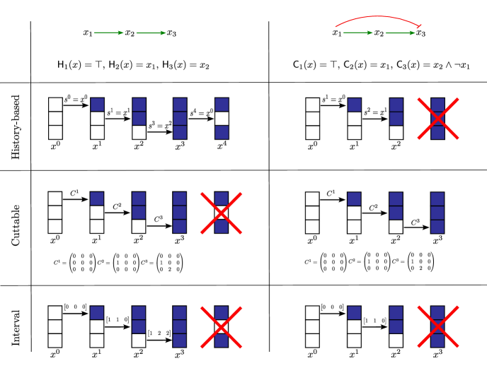
Figure 2: Possible trajectories of certain BNs according to different update modes.

The rest of this subsection is devoted to the proof of Theorem 3.1, broken down into items a to h.

1. $\mathtt{A}\subseteq\mathtt{H}\subseteq\mathtt{T}\subseteq\mathtt{S}$ and hence $\mathtt{A}^{*}\subseteq\mathtt{H}^{*}\subseteq\mathtt{T}^{*}\subseteq\mathtt{S}^{*}$.

This follows from the definitions of the different update modes.

1. $\mathtt{H}\subseteq\mathtt{M}\subseteq\mathtt{S}$ and hence $\mathtt{H}^{*}\subseteq\mathtt{M}^{*}\subseteq\mathtt{S}^{*}$.

Again, this follows from the definitions of the different update modes.

1. $\mathtt{A}\subseteq\mathtt{I}\subseteq\mathtt{C}\subseteq\mathtt{M}$ and hence $\mathtt{A}^{*}\subseteq\mathtt{I}^{*}\subseteq\mathtt{C}^{*}\subseteq\mathtt{M}^{*}$.

Indeed, an $\mathtt{A}$-trajectory is an $\mathtt{I}$-trajectory with $V^{a}_{j}=a-1$ for all $a\geq 1$ and $j\in[n]$; an $\mathtt{I}$-trajectory is a $\mathtt{C}$-trajectory with $C^{a}_{j,i}=V^{a}_{j}$ for all $0\leq a\leq l$ and $j,i\in[n]$; and a $\mathtt{C}$-trajectory is an $\mathtt{M}$-trajectory since $s^{a}\in[x^{0},\dots,x^{a-1}]$ for all $1\leq a\leq l$.

1. $\mathtt{I}\not\subseteq\mathtt{T}$.

Example 3.2 (An interval trajectory that is not trapping).

Let $\mathsf{I}$ be the network from Example 2.6. Then we claim that $(000,100,101,111,011)$ is an $\mathtt{I}$-trajectory but not a $\mathtt{T}$-trajectory.

We have already shown that it is an $\mathtt{I}$-trajectory. It is not a $\mathtt{T}$-trajectory, as $x_{1}^{4}\neq x^{3}_{1}$ implies that $i^{4}=1$, while $\mathsf{I}_{1}(x^{0})=\mathsf{I}_{1}(x^{1})=\mathsf{I}_{1}(x^{2})=\mathsf{I}_{1}(x^{3})=1$ implies that $s^{4}\notin\{x^{0},\dots,x^{3}\}$.

1. $\mathtt{T}^{*}=\mathtt{S}^{*}$.

We now prove that the trapping update mode and the subcube-based update mode allow to reach any configuration in the whole principal trapspace.

Proposition 3.3.

For all $f\in\mathrm{F}(n)$, and all $x,y\in\mathbb{B}^{n}$, the following are equivalent:

1. $y$ is reachable from $x$ by trapping updates, i.e. $x\to^{*}_{\mathtt{T}}y$;

2. $y$ is reachable from $x$ by subcube-based updates, i.e. $x\to^{*}_{\mathtt{S}}y$;

3. $y\in T_{f}(x)$.

Proof.

$\ref{item:reachable_trapping}\implies\ref{item:reachable_subcube}$. Trivial.

$\ref{item:reachable_subcube}\implies\ref{item:in_trapspace}$. Let $x=x^{0}\to_{\mathtt{S}}\dots\to_{\mathtt{S}}x^{l}=y$. We prove that $x^{a}\in T_{f}(x)$ by induction on $0\leq a\leq l$. The case $a=0$ is trivial, therefore suppose it holds for up to $a-1$. We have $s^{a},t^{a}\in[x^{0},\dots,x^{a-1}]\subseteq T_{f}(x)$. Let $u^{a}=f(s^{a})$, then again $u^{a}\in T_{f}(x)$ since $T_{f}(x)$ is a trapspace. We obtain

$$x^{a}=(f_{i^{a}}(s^{a}),t^{a}_{-i^{a}})=(u^{a}_{i^{a}},t^{a}_{-i^{a}})\in[u^{a},t^{a}]\subseteq T_{f}(x).$$

$\ref{item:in_trapspace}\implies\ref{item:reachable_trapping}$. We first prove that if $y$ is reachable from $x$ by trapping updates, then any $z\in[x,y]$ is reachable from $x$. Let $x=x^{0}\to_{\mathtt{T}}\dots\to_{\mathtt{T}}x^{l}=y$, then for all $j\in\Delta(x,y)$, there exists $0\leq b(j)\leq l-1$ such that $y_{j}=f_{j}(x^{b(j)})$ (since the source $s^{a}$ always belongs to $\{x^{0},\dots,x^{l-1}\}$). Therefore, one can reach $z$ by extending the trajectory as follows: if $\Delta(x,z)=\{j_{1},\dots,j_{k}\}$, let $w^{l+a}=(j_{a},b(j_{a}),x)$ for $1\leq a\leq k$, then $x^{l+k}=z$. Therefore, the set $\{y:x\to_{\mathtt{T}}^{*}y\}$ of configurations reachable from $x$ is a subcube. We now prove that if $y$ is reachable from $x$, then $f(y)$ is also reachable from $x$. Let $x=x^{0}\to_{\mathtt{T}}\dots\to_{\mathtt{T}}x^{l}=y$ and define $w^{l+j}=(i^{l+j}=j,s^{l+j}=y,t^{l+j}=x^{l+j-1})$ for all $j\in[n]$; it is then easy to verify that $x^{l+n}=f(y)$. Thus $\{y:x\to_{\mathtt{T}}^{*}y\}$ is a trapspace containing $x$, and hence it contains $T_{f}(x)$. ∎

1. $\mathtt{I}^{*}\subseteq\mathtt{H}^{*}$.

We first prove two lemmas about history-based and interval trajectories, respectively.

Lemma 3.4.

If $x^{0}\to_{\mathtt{H}}\dots\to_{\mathtt{H}}x^{l}$ is a history-based trajectory, then so is $x^{0}\to_{\mathtt{H}}\dots\to_{\mathtt{H}}x^{l}\to_{\mathtt{H}}x^{l+1}=x^{l}$.

Proof.

Let $w^{l}=(i^{l},s^{l}=x^{l^{\prime}},t^{l}=x^{l-1})$ where $l^{\prime}<l$. Define $w^{l+1}=(i^{l+1}=i^{l},s^{l+1}=s^{l},t^{l+1}=x^{l})$; we then have $x^{l+1}=(f_{i^{l+1}}(s^{l+1})=x^{l}_{i^{l}},t^{l+1}_{-i^{l+1}}=x^{l}_{-i^{l}})=x^{l}$. ∎

Lemma 3.5.

If $x\to_{\mathtt{I}}^{*}y$, there is always an interval trajectory $x=x^{0}\to_{\mathtt{I}}x^{1}\to_{\mathtt{I}}\cdots\to_{\mathtt{I}}x^{p}=y$ with $d_{\mathrm{H}}(s^{a-1},s^{a})\leq 1$ for all $1\leq a\leq p$.

Proof.

Let $x=x^{0}\to_{\mathtt{I}}\dots\to_{\mathtt{I}}x^{l}=y$ be an interval trajectory where $d_{\mathrm{H}}(s^{a-1},s^{a})\leq 1$ for all $1\leq a\leq p-1$ and $d_{\mathrm{H}}(s^{p-1},s^{p})>1$. Let us prove how we can replace the transition $x^{p}\to_{\mathtt{I}}x^{p+1}$ with a sequence of transitions $u^{0}=x^{p}\to_{\mathtt{I}}\dots\to_{\mathtt{I}}u^{n}=x^{p+1}$ and still have an interval trajectory.

For any $0\leq i\leq n$, let $v^{i}$ be the configuration such that $v^{i}_{j}=s^{p}_{j}$ for all $1\leq j\leq i$ and $v^{i}_{j}=s^{p-1}_{j}$ for all $i+1\leq j\leq n$. We then have $d_{\mathrm{H}}(v^{i},v^{i-1})\leq 1$ for all $1\leq i\leq n$. Let $u^{i}$ be recursively defined as $u^{0}=x^{p}$ and $u^{i}=(f_{i}(v^{i-1}),u^{i-1}_{-i})$.

Denote $\dot{x}^{a}=x^{a}$ for all $0\leq a\leq p$, $\dot{x}^{p+i}=u^{i}$ for all $1\leq i\leq n$, $\dot{x}^{a+n}=x^{a+1}$ for all $a\geq p+1$. We prove that

$$\dot{x}^{0}=x^{0}\to\dots\to\dot{x}^{p}=x^{p}=u^{0}\to\dots\to\dot{x}^{p+n}=u^{n}=x^{p+1}\to\dots\to\dot{x}^{l+n-1}=x^{l}$$

is an interval trajectory. The first part, $\dot{x}^{0}\to_{\mathtt{I}}\dots\to_{\mathtt{I}}\dot{x}^{p}$, follows from our hypothesis. For the second part, $\dot{x}^{p}\to_{\mathtt{I}}\dots\to_{\mathtt{I}}\dot{x}^{p+n}$, use $w^{p+i}=(i^{p},v^{i-1},u^{i-1})$. For the third part, $\dot{x}^{p+n}\to_{\mathtt{I}}\dots\to_{\mathtt{I}}\dot{x}^{n+1-l}$, then $\dot{w}^{n-1+a}=w^{a}$ is a valid triple for interval updates. ∎

We can now prove the main result.

Proposition 3.6.

Given two configurations $x$ and $y$, if $x\to_{\mathtt{I}}^{*}y$, then $x\to_{\mathtt{H}}^{*}y$.

Proof.

Let $x=x^{0}\to_{\mathtt{I}}x^{1}\to_{\mathtt{I}}\cdots\to_{\mathtt{I}}x^{l}=y$ be an interval trajectory with corresponding triples $w^{a}=(i^{a},s^{a},t^{a})$ for all $1\leq a\leq l$.

According to Lemma 3.5, we assume $d_{\mathrm{H}}(s^{a-1},s^{a})\leq 1$ for all $1\leq a\leq l$.

We first prove, by induction over $1\leq a\leq l$, that there always exists a history-based trajectory $x=x^{0}\to_{\mathtt{H}}s^{1}\to_{\mathtt{H}}\cdots\to_{\mathtt{H}}s^{a}$. The basic case $a=1$ is trivial because $s^{1}=x^{0}$. Assume the statement holds for $a-1$, i.e. $x=x^{0}\to_{\mathtt{H}}s^{1}\to_{\mathtt{H}}\cdots\to_{\mathtt{H}}s^{a-1}$ is a history-based trajectory. Lemma 3.4 settles the case where $s^{a}=s^{a-1}$, hence we assume $s^{a-1}\neq s^{a}$ and, according to Lemma 3.5, $\Delta(s^{a-1},s^{a})=\{j\}$. Then, for $q=V^{a}_{j}$, we have $q<a$ and $x^{q}_{j}=s^{a}_{j}$. Suppose, for the sake of contradiction, that $x^{m}_{j}=x^{q}_{j}$ for all $0\leq m\leq q$. Then, $s^{m}_{j}=x^{q}_{j}$ for all $0\leq m\leq q$, and in particular $s^{a-1}_{j}=s^{a}_{j}$, which is the desired contradiction. Therefore, there exists $q^{\prime}<q$ such that $f_{j}(s^{q^{\prime}})=x^{q}_{j}$. Thus, let $s^{a}=s^{q^{\prime}}$ and $i^{a}=j$. We obtain $(f_{j}(s^{q^{\prime}})=s^{a}_{j},s^{a-1}_{-j})=s^{a}$.

We now prove that we can extend the history-based trajectory all the way to $y$. More formally, we prove that $x=x^{0}\rightarrow s^{1}\rightarrow\cdots\rightarrow s^{l}\rightarrow\cdots\rightarrow y$ is a history-based trajectory (where $s^{l}\rightarrow\cdots\rightarrow y$ is any geodesic). Let $\Delta=\Delta(s^{l},y).$ For all $j\in\Delta$, there exists $q_{j}<l$ such that $f_{j}(s^{q_{j}})=y_{j}$. Since $s_{j}^{l}=x^{m}_{j}\neq y_{j}$ (for some $m<l$), there exists $q_{j}$ such that $j=i^{q_{j}}$ and $f_{j}(s^{q_{j}})=y_{j}$. Then $x=x^{0}\rightarrow s_{1}\rightarrow\cdots\rightarrow s_{l}\rightarrow g^{l+1}\cdots\rightarrow g^{l+\mid\Delta\mid}=y$ is a history-based trajectory with $\{i^{l+1},\ldots,i^{l+\mid\Delta\mid}\}=\Delta$, and for $l+1\leq m\leq l+\mid\Delta\mid$, let $s^{m}=s^{q_{m}}$ when $f_{i_{m}}(s^{q_{m}})=y_{i_{m}}$ and finally $t^{m}=g^{m-1}$. ∎

1. $\mathtt{T}^{*}\not\subseteq\mathtt{M}^{*}$ and hence $\mathtt{T}\not\subseteq\mathtt{M}$.

All the update modes considered in this paper have the property that trajectories can be compressed. Our definition of trajectory allows for transitions $x^{a-1}\to_{\mu}x^{a}$ where $x^{a-1}=x^{a}$; a simple example is when $x^{a-1}$ is a fixed point of $f$ and $s^{a}=t^{a}=x^{a-1}$. We can compress a trajectory by removing consecutive duplicates and obtain a new trajectory where $x^{a}\neq x^{a-1}$ for all $a\geq 1$. The update modes in this paper then have the following property: if $x=x^{0}\to\dots\to x^{l}=y$ is a $\mu$-trajectory, then so is its compressed version $x=x^{0}\to\dots\to x^{m}=y$. This property is easy but tedious to prove; as such we shall omit the proof.

For this and the following items, we aim to prove that for a given pair $x,y$ of configurations, there is no trajectory from $x$ to $y$ in a particular update mode (for this item, the most permissive update mode). Based on the considerations above, we always prove that there is no compressed trajectory from $x$ to $y$ in a particular update mode.

Example 3.7 (A trapping reachability pair that is not most permissive).

Let $\mathsf{T}$ be the network from Example 2.3. We claim that $(00,01)$ is a $\mathtt{T}$-reachability pair but not a $\mathtt{M}$-reachability pair. First, we have already given a $\mathtt{T}$-trajectory from $00$ to $01$. Second, any $\mathtt{M}$-trajectory starting at $x^{0}=00$ must have $x^{1}=10$. Therefore, any trajectory reaching $y=01$ must have some $a\geq 2$ with $i^{a}=1$ and $\mathsf{T}_{1}(s^{a})=0$, which is the desired contradiction.

1. $\mathtt{H}^{*}\not\subseteq\mathtt{C}^{*}$ and hence $\mathtt{H}\not\subseteq\mathtt{C}$.

Example 3.8 (A history-based reachability pair that is not cuttable).

Let us consider the network $\mathsf{H}$ from Example 2.2, with $\mathsf{H}_{1}(x)=1$, $\mathsf{H}_{2}(x)=x_{1}$ and $\mathsf{H}_{3}(x)=x_{2}$. We have shown that $y=101$ is $\mathtt{H}$-reachable from $x=000$; let us now prove that $y$ is not $\mathtt{C}$-reachable from $x$.

Suppose that there is a trajectory $x=x^{0}\to_{\mathtt{C}}\dots\to_{\mathtt{C}}x^{l}=y$. We start with $x^{0}=000$ with $C^{0}_{i,j}=0$ for all $i,j$. In this network, we must activate the second to activate the third component. For this reason, the first component must be updated. Then, we consider $i^{1}=1$ and $C^{1}=C^{0}$. Accordingly, $s^{1}=x^{0}$ and $x^{1}=100$. Afterwards, to update the second component (i.e., $i^{2}=2$), we must consider $C^{2}_{2,1}=1$ and $C^{2}_{i,j}=C^{1}_{i,j}$ otherwise. As a result, $s^{2}=x^{1}_{1}x^{0}_{2}x^{0}_{3}=100$ and $x^{2}=110$. Later, $x^{3}$ can be calculated with $i^{3}=3$, $C^{3}_{3,2}=2$ and $C^{3}_{i,j}=C^{2}_{i,j}$ otherwise. Accordingly, $s^{3}=x^{1}_{1}x^{2}_{2}x^{0}_{3}=110$ and $x^{3}=111$. At this point, to reach the configuration $101$, we should be able to update the second component by considering a matrix $C^{4}$ where $C^{4}_{2,1}=0$ (to deactivate the second component). However, this is not possible as $C^{4}\geq C^{3}$. In conclusion, $101$ cannot be reached by $000$.

This argument is displayed in the left column of Figure 2.

1. $\mathtt{C}^{*}\not\subseteq\mathtt{H}^{*}$.

Example 3.9 (A cuttable reachability pair that is not history-based).

Let us consider the network $\mathsf{C}$ from Example 2.7 with $\mathsf{C}_{1}(x)=1$, $\mathsf{C}_{2}(x)=x_{1}$ and $\mathsf{C}_{3}(x)=x_{2}\land\neg x_{1}$.

We have shown that $y=111$ is $\mathtt{C}$-reachable from $x=000$; let us now prove that $y$ is not $\mathtt{H}$-reachable from $x$. According to the history-based updates, we can reach $x^{1}=100$ (with $s^{0}=x^{0}$ and $i^{1}=1$) and $x^{2}=110$ (with $s^{2}=x^{1}$ and $i^{2}=2$). However, it is impossible to reach the configuration $010$ (the only configuration that allows the third component to be activated). We can therefore conclude that $111$ is unreachable.

This argument is displayed in the right column of Figure 2.

1. $\mathtt{I}^{*}\not\subseteq\mathtt{A}^{*}$ and hence $\mathtt{I}\not\subseteq\mathtt{A}$.

Example 3.10 (An interval reachability pair that is not asynchronous).

Let us consider the network $\mathsf{I}$ from Example 2.6. We have shown that $y=011$ is reachable from $x=000$ by interval updates. However, it is easily seen that $011$ is not reachable from $000$ by asynchronous updates.

3.2 Refinement of the hierarchy by reachability

We make two notes about the hierarchy by reachability in Figure 1.

The hierarchy by reachability gives $\mathtt{C}^{*}\subseteq\mathtt{M}^{*}$ and $\mathtt{H}^{*}\subseteq\mathtt{M}^{*}$, or in other words a reachability pair that is either history-based or cuttable is most permissive. We now prove that there are most permissive reachability pairs that are neither history-based nor cuttable, i.e. $\mathtt{M}^{*}\neq(\mathtt{H}^{*}\cup\mathtt{C}^{*})$. Let $\mathsf{C}\in\mathrm{F}(3)$ from Example 3.9 and $\mathsf{H}$ from Example 3.8, and let $f\in\mathrm{F}(6)$ be defined by

$$f(x_{123},x_{456})=(\mathsf{C}(x_{123}),\mathsf{H}(x_{456})).$$

Then $(000000,111101)$ is a reachability pair that is most permissive but neither history-based nor cuttable.

Similarly, the hierarchy by reachability gives $\mathtt{I}^{*}\subseteq\mathtt{H}^{*}$ and $\mathtt{I}^{*}\subseteq\mathtt{C}^{*}$, or in other words any interval reachability pair is both history-based and cuttable. We now prove that there are some reachability pairs are both history-based and cuttable but not interval, i.e. $\mathtt{I}^{*}\neq(\mathtt{H}^{*}\cap\mathtt{C}^{*})$. We use a similar example to that above – as each trajectory is not an interval trajectory, but this time, we use a middle component that gets activated when either trajectory is used. The details are given in Figure 3.

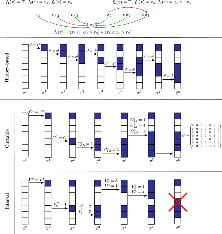
Figure 3: Example of a history-based and cuttable trajectory that is not interval. The example is also valid concerning reachability.

3.3 Equivalent update modes

In Section 3.1, when discussing reachability we only considered the inclusion relation $\mu^{*}\subseteq\nu^{*}$; here we consider two equivalence relations for update modes based on reachability. First, for any $x$, let $\mu^{*}(x)=\{y:x\to_{\mu}^{*}y\}$ be the set of configurations reachable from $x$. Then say two update modes are commensurate if there exist two functions $\phi,\psi:\mathbb{N}\to\mathbb{N}$ such that for all BNs $f$ and all configurations $x$,

$$|\mu^{*}(x)|\leq\phi(|\nu^{*}(x)|),\qquad|\nu^{*}(x)|\leq\psi(|\mu^{*}(x)|).$$

In other words, the number of reachable configurations in one mode gives an estimate of the number of reachable configurations in the other. Second, we say that a configuration $y$ is a min-trapspace configuration if its principal trapspace is minimal. We say $\mu$ and $\nu$ are min-trapspace-equivalent if for all BNs $f$, all configurations $x$, and all min-trapspace configurations $y$, $x\to_{\mu}^{*}y$ if and only if $x\to_{\nu}^{*}y$.

We now classify the commensurate and min-trapspace-equivalent update modes from our list. Since $\mathtt{T}^{*}=\mathtt{S}^{*}$, we omit $\mathtt{S}$.

Theorem 3.11.

Let $\mu,\nu\in\{\mathtt{A},\mathtt{H},\mathtt{T},\mathtt{M},\mathtt{I},\mathtt{C}\}$. The following are equivalent:

1. $\mu$ and $\nu$ are commensurate;

2. $\mu$ and $\nu$ are min-trapspace-equivalent;

3. either $\mu=\nu$ or $\{\mu,\nu\}=\{\mathtt{T},\mathtt{M}\}$.

We first prove that $\mathtt{M}$ is min-trapspace-equivalent to $\mathtt{T}$.

Lemma 3.12.

For any configuration $x$ and any min-trapspace configuration $y\in T_{f}(x)$, we have $x\to_{\mathtt{M}}^{*}y$.

Proof.

We first prove that $x\to_{\mathtt{M}}^{*}u:=T_{f}(x)-x$. Let $z\in T_{f}(x)$ be the furthest configuration reachable from $x$ in $\mathtt{M}$, and let $x=x^{0}\to_{\mathtt{M}}\dots\to_{\mathtt{M}}x^{l-1}=z$. For the sake of contradiction, assume $z\neq u$. Since $[x,z]$ is a strict subcube of $T_{f}(x)$, it is not a trapspace, hence there exists $s^{l}\in[x,z]\subseteq[x^{0},\dots,x^{l-1}]$ such that $f(s^{l})\notin[x,z]$. In particular, there exists a coordinate $i^{l}\in[n]$ such that $x_{i^{l}}=z_{i^{l}}\neq f_{i^{l}}(s^{l})$. Letting $w^{l}=(i^{l},s^{l},t^{l}=z)$, we obtain $x^{l}$ that is reachable from $x$ and yet is further away from $x$ than $z$ is, which is the desired contradiction.

Let $x^{0}=x\to_{\mathtt{M}}\dots\to_{\mathtt{M}}x^{l}=u$. Now, for all $j\in[n]$, there exists $s^{l+j}\in T_{f}(y)$ with $f_{j}(z)=y_{j}$. Indeed, suppose, for the sake of contradiction, that $f_{i}(z)=\neg y_{i}$ for all $z\in T_{f}(y)$. Then the subcube $T_{f}(y)\cap\{x\in\mathbb{B}^{n}:x_{i}=\neg y_{i}\}$ is a trapspace that is strictly contained in $T_{f}(y)$, which is the desired contradiction.

Therefore, the trajectory $x^{0}=x\to_{\mathtt{M}}\dots\to_{\mathtt{M}}x^{l}=u=u^{0}\to_{\mathtt{M}}u^{1}\to_{\mathtt{M}}\dots\to_{\mathtt{M}}u^{n}=y$ is indeed an $\mathtt{M}$-trajectory with $w^{l+j}=(j,s^{l+j},u^{l-1})$ for all $1\leq j\leq n$. ∎

We now prove that trapping and most permissive update modes are commensurate. In fact, we can be a lot more precise.

Proposition 3.13.

For any configuration $x$ with $|\mathtt{T}^{*}(x)|=2^{d}$, then $|\mathtt{M}^{*}(x)|\geq L(d)=2^{\lfloor d/2\rfloor}+2^{\lceil d/2\rceil}-1$. Conversely, for any $L(d)\leq k\leq 2^{d}$, there exists $f\in\mathrm{F}(d)$ and $x\in\mathbb{B}^{d}$ such that $T_{f}(x)=\mathbb{B}^{d}$ while $|\mathtt{M}^{*}(x)|=k$.

Proof.

Without loss, let $d=n$ and $x=0\dots 0$. Let $C$ be the set of local functions $f_{i}$ that are constant (equal to $1$) in $T_{f}(x)=\mathbb{B}^{n}$, and let $c=|C|$ and $D=[n]\setminus C$. Then $x$ can always reach the following two sets of configurations in $\mathtt{M}$.

1. $Y=\{y\in\mathbb{B}^{n}:y_{C}=1\}$. The proof is similar to that of Lemma 3.12: first reach $u=T_{f}(x)-x=1\dots 1$, then for all $i\geq c+1$, there exists $s^{i}$ such that $f_{i}(s^{i})=y_{i}$, hence $y$ can be reached.

2. $Z=\{z\in\mathbb{B}^{n}:z_{D}=0\}$. Any geodesic from $x$ to $z$ is a most permissive trajectory.

We have $|Y|=2^{n-c}$, $|Z|=2^{c}$, and $|Y\cap Z|=1$, thus $x$ can reach at least $2^{n-c}+2^{c}-1\geq L(d)$ configurations.

We prove, by induction on $n$, that for any $L(n)\leq k\leq 2^{n}$ there exists $f\in\mathrm{F}(n)$ and $x\in\mathbb{B}^{n}$ such that $T_{f}(x)=\mathbb{B}^{n}$ and $|\mathtt{M}^{*}(x)|=k$. We also use its immediate consequence: for any $n\geq 1$ and any $1\leq r\leq 2^{n}$, there exists $f\in\mathrm{F}(n)$ and $x\in\mathbb{B}^{n}$ such that $|\mathtt{M}^{*}(x)|=r$. The claim is trivial for $n=1$ so let us assume it holds up to $n-1$. Let $c=\lfloor n/2\rfloor$ and define $q$ and $r$ as the quotient and remainder of the following long division:

$$k+2^{n-c}-2^{c}=q(2^{n-c}-1)+r.$$

Let $Q$ be an up-set of $\mathbb{B}^{c}$ (i.e. if $s\in Q$ and $t\geq s$, then $t\in Q$) with $|Q|=q$ and let $q^{*}$ be a minimal element of $Q$.

By induction hypothesis, let $g\in\mathrm{F}(n-c)$ and $z=0\dots 0\in\mathbb{B}^{n-c}$ such that $|\mathtt{M}^{*}(z)|=r$. Let $C=\{1,\dots,c\}$ and $D=\{c+1,\dots,n\}$ and let $f\in\mathrm{F}(n)$ be defined as

$$f_{C}(x) =1_{C},$$

$$f_{D}(x) =\begin{cases}\neg x_{D}&\text{if }x_{C}\in Q\setminus\{q^{*}\}\\ g(x_{D})&\text{if }x_{C}=q^{*}\\ x_{D}&\text{if }x_{D}\notin Q.\end{cases}$$

Since the local functions in $C$ are constant and equal to $1$, any $\mathtt{M}$-trajectory is monotone with respect to $x_{C}$, i.e. if $x^{0}\to_{\mathtt{M}}\dots\to_{\mathtt{M}}x^{l}$, then $x^{0}_{C}\leq\dots\leq x^{l}_{C}$. For any $\alpha\in\mathbb{B}^{c}$, let $R_{\alpha}=\{y\in\mathtt{M}^{*}(x):y_{C}=\alpha\}$; then $R_{\alpha}=\bigcup_{\beta\leq\alpha}R_{\beta}$.

We can now determine the configurations reachable from $x$. Firstly, if $\alpha\in\mathbb{B}^{c}\setminus Q$, then $f_{D}(\alpha,x_{D})$ reduces to the identity, hence $R_{\alpha}=\{(\alpha,z)\}$. Secondly, if $\alpha=q^{*}$, then $f_{C}(\alpha,x_{D})$ reduces to $g$, hence $R_{q^{*}}=\{(q^{*},b):b\in\mathtt{M}^{*}(z)\}$. Thirdly, if $\alpha\in Q\setminus\{q^{*}\}$, then $f_{D}(\alpha,x_{D})$ reduces to the negation, hence $R_{\alpha}=\{(\alpha,a):a\in\mathbb{B}^{n-c}\}$. Therefore, $x$ reaches the following set of configurations:

$$\mathtt{M}^{*}(x) =\{(\alpha,z):\alpha\in\mathbb{B}^{c}\setminus Q\}\cup\{(q^{*},b):b\in\mathtt{M}^{*}(z)\}\cup\{(\alpha,a):\alpha\in Q\setminus\{q^{*}\},a\in\mathbb{B}^{n-c}\},$$

whence $|\mathtt{M}^{*}(x)|=(2^{c}-q)+r+2^{n-c}(q-1)=k$. ∎

We now exhibit some min-trapspace configurations that are reachable in some update mode $\mu$ but not in another mode $\nu$. Those examples also show that $\mu$ and $\nu$ are not commensurate. The three examples below follow a similar structure; as such, we only provide a detailed explanation for the first example.

Example 3.14 (Min-trapspace configurations reachable in history-based but not in cuttable).

Let $\mathsf{H}\in\mathrm{F}(3)$ be the network from Example 2.2 and let $s=101$. It is easily seen that there is no $\mathtt{C}$-trajectory such that $s^{a}=s$. Then let $\hat{\mathsf{H}}\in\mathrm{F}(n)$ be defined as

$$\hat{\mathsf{H}}(x)=\begin{cases}(\neg x_{123},\neg x_{4..n-1},1)&\text{if }x_{n}=1\\ (\mathsf{H}(x_{123}),0_{4..n-1},0)&\text{if }x_{n}=0\text{ and }x_{4..n-1}=0\text{ and }x_{123}\neq s\\ (\mathsf{H}(s),0_{4..n-1},1)&\text{if }x_{n}=0\text{ and }x_{4..n-1}=0\text{ and }x_{123}=s\\ x&\text{otherwise}.\end{cases}$$

Note that there is only one transition from the hyperplane $\{x\in\mathbb{B}^{n}:x_{n}=0\}$ to its parallel $\{x\in\mathbb{B}^{n}:x_{n}=1\}$. Then $\hat{x}=0\dots 0$ can reach the whole of $\{x\in\mathbb{B}^{n}:x_{n}=0\}$ in $\mathtt{H}$ but it can only reach as most the seven configurations $\{(y_{123},0_{4..n-1},0):y\neq s\}$ in $\mathtt{C}$.

Example 3.15 (Min-trapspace configurations reachable in cuttable but not in history-based or interval).

Let $\mathsf{C}\in\mathrm{F}(3)$ be the network from Example 2.7 and $s=010$, then again no history-based or interval trajectory can have $s^{a}=s$. Then let $\hat{\mathsf{C}}\in\mathrm{F}(n)$ be defined as

$$\hat{\mathsf{C}}(x)=\begin{cases}(\neg x_{123},\neg x_{4..n-1},1)&\text{if }x_{n}=1\\ (\mathsf{C}(x_{123}),0_{4..n-1},0)&\text{if }x_{n}=0\text{ and }x_{4..n-1}=0\text{ and }x_{123}\neq s\\ (\mathsf{C}(s),0_{4..n-1},1)&\text{if }x_{n}=0\text{ and }x_{4..n-1}=0\text{ and }x_{123}=s\\ x&\text{otherwise}.\end{cases}$$

The two previous examples also prove that $\mathtt{M}$ is not min-trapspace equivalent to either $\mathtt{C}$ or $\mathtt{H}$.

Example 3.16 (Min-trapspace configurations reachable in interval but not in asynchronous).

Let $\mathsf{I}\in\mathrm{F}(2)$ be the network from Example 3.10. Let $s=01$ and $\hat{\mathsf{I}}\in\mathrm{F}(n)$ be defined as

$$\hat{\mathsf{I}}(x)=\begin{cases}(\neg x_{12},\neg x_{3..n-1},1)&\text{if }x_{n}=1\\ (\mathsf{I}(x_{12}),0_{3..n-1},0)&\text{if }x_{n}=0\text{ and }x_{3..n-1}=0\text{ and }x_{12}\neq s\\ (\mathsf{I}(s),0_{3..n-1},1)&\text{if }x_{n}=0\text{ and }x_{3..n-1}=0\text{ and }x_{12}=s\\ x&\text{otherwise}.\end{cases}$$

4 Principal trapspaces

4.1 Principal trapspaces and trapping closure

The general asynchronous graph of a BN $f\in\mathrm{F}(n)$ is the graph $\mathtt{GA}(f)=(V,E)$ where $V=\mathbb{B}^{n}$ and

$$E=\{(x,f^{(S)}(x)):x\in\mathbb{B}^{n},S\subseteq[n]\}.$$

It is clear that the mapping $\mathtt{GA}:f\mapsto\mathtt{GA}(f)$ is injective. We first characterise the general asynchronous graphs.

Proposition 4.1.

Let $\Gamma$ be a graph on $\mathbb{B}^{n}$. Then $\Gamma=\mathtt{GA}(f)$ for some $f\in\mathrm{F}(n)$ if and only if $\Gamma$ is reflexive and all out-neighbourhoods are subcubes.

Proof.

We have $N^{out}(\mathtt{GA}(f);x)=[x,f(x)]$ for all $x$, i.e. $\mathtt{GA}(f)$ is reflexive and all out-neighbourhoods are subcubes. Conversely, if $\Gamma$ is reflexive and all out-neighbourhoods are subcubes, then $\Gamma=\mathtt{GA}(f)$, where $f(x)=N^{out}(\Gamma;x)-x$ for all $x$. ∎

Example 4.2.

Let $f\in\mathrm{F}(3)$ be the BN in Example 1.1. The general asynchronous graph of $f$ is given as follows. The blue arrows come from $\mathtt{A}(f)$ while the magenta arrows are additional transitions in $\mathtt{GA}(f)$; once again we omit the loops on all the vertices.

Say a BN $g$ is trapping if $\mathtt{GA}(g)$ is transitive. Denote the set of all trapping BNs in $\mathrm{F}(n)$ as ${\mathrm{F}}^{\mathrm{T}}(n)$. We explain this terminology and characterise trapping networks in the rest of this subsection.

The trapping graph of a BN $f\in\mathrm{F}(n)$ is the graph $\mathtt{T}(f)=(V,E)$ where $V=\mathbb{B}^{n}$ and

$$E=\{(x,y):x\in\mathbb{B}^{n},y\in T_{f}(x)\}.$$

If $y\in T_{f}(x)$, then $T_{f}(x)$ is a trapspace of $f$ containing $y$, thus $T_{f}(y)\subseteq T_{f}(x)$; in other words, the trapping graph is transitive. In $\mathtt{T}(f)$, the out-neighbourhood of $x$ is a subcube containing $x$. Let ${f}^{\mathrm{T}}\in\mathrm{F}(n)$ be the BN that maps $x$ to its opposite in that subcube, i.e.

$${f}^{\mathrm{T}}(x)=T_{f}(x)-x,$$

so that $T_{f}(x)=[x,{f}^{\mathrm{T}}(x)]$. We refer to ${f}^{\mathrm{T}}$ as the trapping closure of $f$.

Example 4.3.

Let $f\in\mathrm{F}(3)$ be the BN from Examples 1.1 and 4.2. The trapping graph of $f$ is given as follows. The blue arrows come from $\mathtt{A}(f)$, the magenta arrows are additional transitions in $\mathtt{GA}(f)$, while the orange arrows are additional transitions in $\mathtt{T}(f)$; once again we omit the loops on all the vertices.

The asynchronous graph of ${f}^{\mathrm{T}}$ is given as follows, where the blue arrows come from $\mathtt{A}(f)$, while the additional transitions in $\mathtt{A}({f}^{\mathrm{T}})$ are highlighted in cyan.

We now justify the term “trapping closure” used above. Consider the relation on $\mathrm{F}(n)$ given by $f\sqsubseteq g$ if $\Delta(x,f(x))\subseteq\Delta(x,g(x))$ for all $x\in\mathbb{B}^{n}$; or equivalently $\mathtt{GA}(f)\subseteq\mathtt{GA}(g)$. The $\sqsubseteq$ partial order induces a lattice $\mathcal{L}=(\mathrm{F}(n),\sqcup,\sqcap,\mathbf{0},\mathbf{1})$ with

$$\mathtt{GA}(f\sqcup g) =\mathtt{GA}(f)\cup\mathtt{GA}(g)$$

$$\mathtt{GA}(f\sqcap g) =\mathtt{GA}(f)\cap\mathtt{GA}(g)$$

$$\mathbf{0} =\mathrm{id}$$

$$\mathbf{1} =\neg.$$

Proposition 4.4.

The operator $f\mapsto{f}^{\mathrm{T}}$ is a closure operator on $\mathcal{L}$: for all $f,g\in\mathrm{F}(n)$ we have

$$f \sqsubseteq{f}^{\mathrm{T}}$$ (1)

$$f\sqsubseteq g \implies{f}^{\mathrm{T}}\sqsubseteq{g}^{\mathrm{T}}$$ (2)

$${({f}^{\mathrm{T}})}^{\mathrm{T}} ={f}^{\mathrm{T}}.$$ (3)

Proof.

(1). Since $f(x)\in T_{f}(x)$ for all $x$, we obtain $f\sqsubseteq{f}^{\mathrm{T}}$.

(2). Suppose $f\sqsubseteq g$, then we need to prove that $T_{f}(x)\subseteq T_{g}(x)$ for all $x\in\mathbb{B}^{n}$. For all $y\in T_{g}(x)$, we have $[y,g(y)]\subseteq T_{g}(x)$ hence $[y,f(y)]\subseteq T_{g}(x)$. Thus $T_{g}(x)$ is a trapspace of $f$ containing $x$ whence $T_{f}(x)\subseteq T_{g}(x)$.

(3). Let $g={f}^{\mathrm{T}}$. We prove that $T_{g}(x)=T_{f}(x)$ for all $x\in\mathbb{B}^{n}$. Firstly, $T_{f}(x)\subseteq T_{g}(x)$ because $f\sqsubseteq g$. Conversely, for any $y\in T_{f}(x)$, we have $T_{f}(y)=[y,g(y)]\subseteq T_{f}(x)$, hence $g(y)\in T_{f}(x)$. Therefore $T_{f}(x)$ is a trapspace of $g$ containing $y$, thus $T_{g}(x)\subseteq T_{f}(x)$. ∎

We can now give an algebraic characterisation of ${f}^{\mathrm{T}}$.

Corollary 4.5.

For all $f\in\mathrm{F}(n)$ we have

$${f}^{\mathrm{T}}=\bigsqcap\{g\in{\mathrm{F}}^{\mathrm{T}}(n):f\sqsubseteq g\}.$$

Proof.

Immediately follows from [6, Theorem 1.1] applied to $\mathcal{L}$. ∎

We now obtain the following characterisation of trapping networks.

Proposition 4.6.

For all $g\in\mathrm{F}(n)$, the following are equivalent:

1. $g$ is trapping, i.e. $\mathtt{GA}(g)$ is transitive,

2. $g={g}^{\mathrm{T}}$,

3. $g={f}^{\mathrm{T}}$ for some $f$,

4. $\mathtt{T}(g)=\mathtt{GA}(g)$,

5. $\Delta(y,g(y))\subseteq\Delta(x,g(x))$ for all $x\in\mathbb{B}^{n}$ and $y\in[x,g(x)]$.

Proof.

$\ref{item:g_trapping}\iff\ref{item:g=gt}$. We have

$$g\text{ trapping } \iff\forall x\in\mathbb{B}^{n}\ \ \forall y\in[x,g(x)]\ \ g(y)\in[x,g(x)]$$

$$\iff\forall x\in\mathbb{B}^{n}\ \ [x,g(x)]\in\mathcal{T}(g)$$

$$\iff\forall x\in\mathbb{B}^{n}\ \ [x,g(x)]=T_{g}(x)$$

$$\iff g={g}^{\mathrm{T}}.$$

$\ref{item:g=gt}\implies\ref{item:g=ft}$. Trivial.

$\ref{item:g=ft}\implies\ref{item:g_trapping}$. If $g={f}^{\mathrm{T}}$, then $\mathtt{GA}(g)=\mathtt{GA}({f}^{\mathrm{T}})=\mathtt{T}(f)$ is transitive.

$\ref{item:TG(g)=GA(g)}\iff\ref{item:g=gt}$. We have $\mathtt{T}(g)=\mathtt{GA}(g)$ if and only if $\mathtt{GA}(g)=\mathtt{GA}({g}^{\mathrm{T}})$, which in turn is equivalent to $g={g}^{\mathrm{T}}$.

$\ref{item:delta(y,g(y))}\iff\ref{item:g=gt}$. For all $g\in\mathrm{F}(n)$ and $x\in\mathbb{B}^{n}$, we have

$$\Delta(y,g(y))\subseteq\Delta(x,g(x))\forall y\in[x,g(x)] \iff[y,g(y)]\subseteq[x,g(x)]\forall y\in[x,g(x)]$$

$$\iff g(y)\in[x,g(x)]\forall y\in[x,g(x)]$$

$$\iff[x,g(x)]=T_{g}(x)$$

$$\iff g(x)={g}^{\mathrm{T}}(x).$$

∎

Proposition 4.6 yields the following corollary.

Corollary 4.7.

For all $f\in\mathrm{F}(n)$,

$$\mathtt{T}(f)=\mathtt{GA}({f}^{\mathrm{T}})=\mathtt{T}({f}^{\mathrm{T}}).$$

We can also classify the trapping graphs as the transitive general asynchronous graphs.

Corollary 4.8.

Let $\Gamma$ be graph on $\mathbb{B}^{n}$. Then $\Gamma=\mathtt{T}(f)$ for some $f\in\mathrm{F}(n)$ if and only if $\Gamma$ is reflexive transitive and all out-neighbourhoods are subcubes.

Proof.

By Proposition 4.1, $\Gamma$ is reflexive transitive and all out-neighbourhoods are subcubes if and only if it is a transitive general asynchronous graph, i.e. $\Gamma=\mathtt{GA}(g)$ for some trapping network $g$. By Corollary 4.7, this is equivalent to $\Gamma=\mathtt{T}(f)$ for some BN $f$. ∎

Trapping graphs form a rich class of graphs. For instance, any $X\subseteq\mathbb{B}^{n}$ can appear as an initial strong component of some trapping graph (namely, for $f(x)=\neg x$ if $x\in X$ and $f(x)=x$ otherwise). Note, however, that if $\mathtt{T}(f)$ has two distinct strong components $S,T$ with $S\to T$, then $[T]\subset[S]$.

We end this subsection with a characterisation of BNs that have the same collection of trapspaces. Recall that the collection of all trapspaces of $f$ is denoted by $\mathcal{T}(f)$, while the collection of all principal trapspaces of $f$ is denoted by $\mathcal{P}(f)$. We note that $\mathcal{P}(f)(x)=\mathcal{T}(f)(x)=T_{f}(x)$.

Theorem 4.9.

Let $f,g\in\mathrm{F}(n)$. The following are equivalent:

1. $\mathcal{P}(f)=\mathcal{P}(g)$;

2. $\mathcal{T}(f)=\mathcal{T}(g)$;

3. $T_{f}(x)=T_{g}(x)$ for all $x\in\mathbb{B}^{n}$;

4. $\mathtt{T}(f)=\mathtt{T}(g)$;

5. ${f}^{\mathrm{T}}={g}^{\mathrm{T}}$.

Proof.

$\ref{item:T(f)=T(g)}\implies\ref{item:Tf(x)=Tg(x)}$. Let $x\in\mathbb{B}^{n}$. On the one hand, since $T_{f}(x)$ and $T_{g}(x)$ are trapspaces of $f$ containing $x$, we have $T_{f}(x)\subseteq T_{g}(x)$. We similarly obtain $T_{g}(x)\subseteq T_{f}(x)$, and hence $T_{f}(x)=T_{g}(x)$.

$\ref{item:Tf(x)=Tg(x)}\implies\ref{item:tau(f)=tau(g)}$. We have

$$A\in\mathcal{T}(f)\iff A=\bigcup\{T_{f}(x):x\in A\}\iff A=\bigcup\{T_{g}(x):x\in A\}\iff A\in\mathcal{T}(g).$$

$\ref{item:tau(f)=tau(g)}\implies\ref{item:T(f)=T(g)}$. Trivial.

$\ref{item:Tf(x)=Tg(x)}\iff\ref{item:TG(f)=TG(g)}\iff\ref{item:fT=gT}$. Immediate from the definitions of $\mathtt{T}(f)$ and ${f}^{\mathrm{T}}$. ∎

Corollary 4.10.

For any BN $f$, $\mathcal{P}(f)=\mathcal{P}({f}^{\mathrm{T}})$ and $\mathcal{T}(f)=\mathcal{T}({f}^{\mathrm{T}})$.

4.2 Classification of collections of (principal) trapspaces

A pre-order on a set $\Omega$ is a reflexive transitive binary relation on $\Omega$. If $R$ is a pre-order on $\Omega$, then any set of the form $S^{\downarrow}=\{y\in\Omega:\exists s\in S,(s,y)\in R\}$ is an ideal of $R$. A principal ideal of $R$ is any set of the form $x^{\downarrow}=\{y\in\Omega,(x,y)\in R\}$. Since $R=\bigcup_{x\in\Omega,y\in x^{\downarrow}}(x,y)$, we see that $R$ can be reconstructed from its collection of principal ideals; the same can be said for its collection of ideals. It is well known that a collection of subsets of $\Omega$ is the collection of ideals of a pre-order if and only if it is closed under arbitrary unions and intersections; similarly one can classify the collections of principal ideals of pre-orders. Therefore, for the set $\Omega$, there is a three-way equivalence between the following three sets: the family of all pre-orders $R$ on $\Omega$, the family of all collections of ideals of pre-orders on $\Omega$, and the family of all collections of principal ideals of pre-orders on $\Omega$.

In this paper, we are interested in $\Omega=\mathbb{B}^{n}$, but we do not consider any possible (principal) ideal. Let $f\in\mathrm{F}(n)$ be a BN. Then the reachability relation $R$ given by $R=\{(x,y):x\to_{\mathtt{GA}(f)}^{*}y\}$ is a pre-order on $\mathbb{B}^{n}$. A subcube is an ideal of $R$ if and only if it is a trapspace of $f$; it is a principal ideal of $R$ if and only if it is a principal trapspace of $f$. The relation $R^{\prime}$ given by $y\in T_{f}(x)$ is also a pre-order, described by the trapping graph ($(x,y)\in R^{\prime}$ if and only if $(x,y)$ is an edge of $\mathtt{T}(f)$). This is the smallest pre-order such that all its principal ideals are principal trapspaces of $f$. So the main result is a three-way equivalence between the following three sets: the family of all trapping networks, the family of all collections of trapspaces, and the family of all collections of principal trapspaces.

Say a collection $\mathcal{J}$ of subcubes is ideal if it is the collection of trapspaces of a BN. We denote the set of all ideal collections of subcubes of $\mathbb{B}^{n}$ as $\mathrm{A}^{\mathcal{T}}(n)$. Accordingly, say a collection $\mathcal{Q}$ of subcubes is principal if it is the collection of principal trapspaces of a BN and denote the set of all principal collections of subcubes of $\mathbb{B}^{n}$ as $\mathrm{A}^{\mathcal{P}}(n)$. We shall give combinatorial descriptions of ideal and principal collections of subcubes in the sequel.

Define the mapping $F:\mathrm{A}(n)\to\mathrm{F}(n)$ as follows. Let $\mathcal{A}\in\mathrm{A}(n)$ be a collection of subcubes of $\mathbb{B}^{n}$. For any $x\in\mathbb{B}^{n}$, denote the intersection of all the subcubes in $\mathcal{A}$ that contain $x$ by

$$\mathcal{A}(x):=\bigcap\{A\in\mathcal{A}:x\in A\},$$

where $\mathcal{A}(x)=\mathbb{B}^{n}$ if the intersection is empty. Then let $F(\mathcal{A})$ be the BN defined by

$$F(\mathcal{A})(x)=\mathcal{A}(x)-x,$$

or equivalently $\mathcal{A}(x)=[x,F(\mathcal{A})(x)]$, for all $x\in\mathbb{B}^{n}$. Let $F_{\mathcal{P}}$ be the restriction of $F$ to $\mathrm{A}^{\mathcal{P}}(n)$ and $F_{\mathcal{T}}$ be the restriction of $F$ to $\mathrm{A}^{\mathcal{T}}(n)$.

Theorem 4.11.

The mapping $F_{\mathcal{P}}$ is a bijection from $\mathrm{A}^{\mathcal{P}}(n)$ to ${\mathrm{F}}^{\mathrm{T}}(n)$; its inverse is the mapping $\mathcal{P}$. That is, for all $\mathcal{Q}\in\mathrm{A}^{\mathcal{P}}(n)$ and all $g\in{\mathrm{F}}^{\mathrm{T}}(n)$, we have

$$\mathcal{P}(F_{\mathcal{P}}(\mathcal{Q}))=\mathcal{Q},\qquad F_{\mathcal{P}}(\mathcal{P}(g))=g.$$

Similarly, the mapping $F_{\mathcal{T}}$ is a bijection from $\mathrm{A}^{\mathcal{T}}(n)$ to ${\mathrm{F}}^{\mathrm{T}}(n)$; its inverse is the mapping $\mathcal{T}$. That is, for all $\mathcal{J}\in\mathrm{A}^{\mathcal{T}}(n)$ and all $g\in{\mathrm{F}}^{\mathrm{T}}(n)$, we have

$$\mathcal{T}(F_{\mathcal{T}}(\mathcal{J}))=\mathcal{J},\qquad F_{\mathcal{T}}(\mathcal{T}(g))=g.$$

The rest of this subsection is devoted to classifying the collections of (principal) trapspaces and to proving the three-way equivalence described above.

Let $\mathcal{Q}\in\mathrm{A}(n)$ be a collection of subcubes of $\mathbb{B}^{n}$. We say $\mathcal{Q}$ is pre-principal if

$$\mathcal{Q}=\{\mathcal{Q}(x):x\in\mathbb{B}^{n}\}.$$

Intuitively, $\mathcal{Q}$ is pre-principal if for any configuration $x$, there exists a smallest subcube in $\mathcal{Q}$ that contains $x$, and conversely for any subcube $A\in\mathcal{Q}$, there is a configuration $x$ for which $A$ is the smallest subcube that contains $x$.

Lemma 4.12.

A collection $\mathcal{Q}$ of subcubes of $\mathbb{B}^{n}$ is pre-principal if and only if the following hold:

1. $\bigcup\mathcal{Q}=\mathbb{B}^{n}$;

2. for all $A,B\in\mathcal{Q}$, there exists $\mathcal{C}\subseteq\mathcal{Q}$ such that $\bigcup\mathcal{C}=A\cap B$;

3. for all $A\in\mathcal{Q}$ and $\mathcal{C}\subseteq\mathcal{Q}$, $\bigcup\mathcal{C}=A$ implies $A\in\mathcal{C}$.

Proof.

Suppose $\mathcal{Q}$ is pre-principal. We prove that it satisfies all three properties.

1. We have $x\in\mathcal{Q}(x)$ for all $x\in\mathbb{B}^{n}$, hence $\bigcup\mathcal{Q}=\mathbb{B}^{n}$.

2. For all $A,B\in\mathcal{Q}$, $\bigcup\{\mathcal{Q}(x):x\in A\cap B\}=A\cap B$.

3. Suppose $\mathcal{C}\subseteq\mathcal{Q}$ with $\bigcup\mathcal{C}=A\in\mathcal{Q}$ while $A\notin\mathcal{C}$. Then for all $x\in A$, there exists $C\in\mathcal{C}$ such that $\mathcal{Q}(x)\subseteq C\subset A$. Therefore, $A\notin\{\mathcal{Q}(x):x\in\mathbb{B}^{n}\}$, which contradicts the fact that $\mathcal{Q}$ is pre-principal.

Conversely, let $\mathcal{Q}$ satisfy all three properties. We first prove that $\mathcal{Q}(x)\in\mathcal{Q}$ for all $x\in\mathbb{B}^{n}$. Let $x\in\mathbb{B}^{n}$ and consider the collection

$$\mathcal{S}=\{A\in\mathcal{Q}:x\in A;\forall B\subset A,B\in\mathcal{Q},x\notin B\}$$

of minimal subcubes in $\mathcal{Q}$ that contain $x$. By Property 1, $|\mathcal{S}|\geq 1$. If $|\mathcal{S}|\geq 2$, let $A,B\in\mathcal{S}$, then there exists $\mathcal{C}\subseteq\mathcal{Q}$ such that $\bigcup\mathcal{C}=A\cap B$. As such, there exists $C\in\mathcal{C}$ such that $x\in C$ while $C\subseteq A\cap B\subset A$, which contradicts the fact that $A\in\mathcal{S}$. Therefore, $|\mathcal{S}|=1$, hence $\mathcal{S}=\{\mathcal{Q}(x)\}$.

We now prove that $A\in\{\mathcal{Q}(x):x\in\mathbb{B}^{n}\}$ for all $A\in\mathcal{Q}$. Let $A\in\mathcal{Q}$, and suppose that $\mathcal{Q}(x)\subset A$ for all $x\in A$. Then $\mathcal{C}:=\{\mathcal{Q}(x):x\in A\}\subset\mathcal{Q}$ satisfies $\bigcup\mathcal{C}=A$ while $A\notin\mathcal{C}$, which contradicts the third property. ∎

Lemma 4.13.

A collection of subcubes is principal if and only if it is pre-principal. For all $\mathcal{Q}\in\mathrm{A}^{\mathcal{P}}(n)$ and all $g\in{\mathrm{F}}^{\mathrm{T}}(n)$, we have

$$\mathcal{P}(F_{\mathcal{P}}(\mathcal{Q}))=\mathcal{Q},\qquad F_{\mathcal{P}}(\mathcal{P}(g))=g.$$

Proof.

Firstly, we prove that $F_{\mathcal{P}}(\mathcal{Q})$ is trapping. Placing ourselves in the graph $\Gamma=\mathtt{GA}(F_{\mathcal{P}}(\mathcal{Q}))$, if $y\in N^{out}(x)=\mathcal{Q}(x)$, then $N^{out}(y)=\mathcal{Q}(y)\subseteq\mathcal{Q}(x)=N^{out}(x)$, and hence $\Gamma$ is transitive.

Secondly, we prove that $\mathcal{P}(g)$ is pre-principal by verifying that it satisfies the three properties of Lemma 4.12. First, since $x\in T_{g}(x)$ for all $x\in\mathbb{B}^{n}$, we have $\bigcup\mathcal{P}(g)=\mathbb{B}^{n}$. Second, for all $A,B\in\mathcal{P}(g)$, the collection $\mathcal{C}=\{T_{g}(x):x\in A\cap B\}$ satisfies $\mathcal{C}\subseteq\mathcal{P}(g)$ and $\bigcup\mathcal{C}=A\cap B$. Third, if there exists $x\in\mathbb{B}^{n}$ and $\mathcal{C}\subseteq\mathcal{P}(g)\setminus\{T_{g}(x)\}$ such that $\bigcup\mathcal{C}=T_{g}(x)$, then there exists $C\in\mathcal{C}$ such that $x\in C\subset T_{g}(x)$ and hence $T_{g}(x)\subseteq C\subset T_{g}(x)$, which is the desired contradiction.

Since any principal collection of subcubes is of the form $\mathcal{P}(g)$ for some trapping BN $g$, we have just shown that any principal collection of subcubes is pre-principal.

Thirdly, we prove that $\mathcal{P}(F_{\mathcal{P}}(\mathcal{Q}))=\mathcal{Q}$ for any pre-principal collection $\mathcal{Q}$ of subcubes of $\mathbb{B}^{n}$. Let $g=F(\mathcal{Q})$. Since $g$ is trapping, we have for all $x\in\mathbb{B}^{n}$

$$T_{g}(x)=N^{out}(\mathtt{GA}(g);x)=\mathcal{Q}(x).$$

Hence $\mathcal{P}(g)=\{\mathcal{Q}(x):x\in\mathbb{B}^{n}\}=\mathcal{Q}$ since $\mathcal{Q}$ is pre-principal.

We have just shown that any pre-principal collection of subcubes is principal. Together with the previous item, we have proved that a collection of subcubes is principal if and only if it is pre-principal.

Fourthly, we prove that $F_{\mathcal{P}}(\mathcal{P}(g))=g$ for all $g\in{\mathrm{F}}^{\mathrm{T}}(n)$. Let $\mathcal{Q}=\mathcal{P}(g)$. For all $x\in\mathbb{B}^{n}$, we have

$$T_{g}(x)=\bigcap\{A\in\mathcal{P}(g):x\in A\}=\mathcal{Q}(x)$$

hence $\mathcal{Q}(x)=[x,g(x)]$ (since $g$ is trapping). On the other hand, by definition $\mathcal{Q}(x)=[x,F_{\mathcal{P}}(\mathcal{Q})(x)]$, thus $g=F_{\mathcal{P}}(\mathcal{Q})$. ∎

We say that a collection $\mathcal{J}$ of subcubes is pre-ideal if it satisfies the following three properties:

1. $\mathbb{B}^{n}\in\mathcal{J}$;

2. $\mathcal{J}$ is closed under intersection, i.e. if $A,B\in\mathcal{J}$ and $A\cap B\neq\emptyset$, then $A\cap B\in\mathcal{J}$;

3. for any subcollection $\mathcal{R}\subseteq\mathcal{J}$, if $R=\bigcup\mathcal{R}\in\mathrm{S}(n)$, then $R\in\mathcal{J}$.

Intuitively, a pre-ideal collection of subcubes is closed under arbitrary unions and intersections, so long as those unions and intersections are actual subcubes.

Lemma 4.14.

A collection of subcubes is ideal if and only if it is pre-ideal. For all $\mathcal{J}\in\mathrm{A}^{\mathcal{T}}(n)$ and all $g\in{\mathrm{F}}^{\mathrm{T}}(n)$, we have

$$\mathcal{T}(F_{\mathcal{T}}(\mathcal{J}))=\mathcal{J},\qquad F_{\mathcal{T}}(\mathcal{T}(g))=g.$$

Proof.

The proof uses a similar structure to that of Theorem 4.13.

Firstly, $F_{\mathcal{T}}(\mathcal{J})$ is trapping. (The proof is the same as its counterpart for $F_{\mathcal{P}}(\mathcal{Q})$.)

Secondly, we prove that $\mathcal{T}(g)$ is pre-ideal. Then $\mathbb{B}^{n}$ is a trapspace of $g$ so $\mathbb{B}^{n}\in\mathcal{J}$; if $A$ and $B$ are trapspaces with non-empty intersection, let $x\in A\cap B$, then $g(x)\subseteq A\cap B$, hence $A\cap B$ is also a trapspace; and if $R=\bigcup\mathcal{R}$ for some $\mathcal{R}\subseteq\mathcal{J}$, then for any $x\in R$, there exists $A\in\mathcal{J}$ such that $x\in A$ and hence $g(x)\in A\subseteq R$, thus $R$ is also a trapspace.

Since any ideal collection of subcubes is of the form $\mathcal{T}(g)$ for some trapping BN $g$, we have just shown that any ideal collection of subcubes is pre-ideal.

Thirdly, we prove that $\mathcal{T}(F_{\mathcal{T}}(\mathcal{J}))=\mathcal{J}$ for any pre-ideal collection $\mathcal{J}$ of subcubes of $\mathbb{B}^{n}$. Let $g=F_{\mathcal{T}}(\mathcal{J})$ so that $[x,g(x)]=\mathcal{J}(x)\in\mathcal{J}$ for all $x\in\mathbb{B}^{n}$. Suppose $A\in\mathcal{J}$, then for all $x\in A$, $g(x)\in\mathcal{J}(x)\subseteq A$, hence $A\in\mathcal{T}(g)$. Conversely, suppose $B\in\mathcal{T}(g)$, then $B=\bigcup\{\mathcal{J}(x):x\in B\}$, whence $B\in\mathcal{J}$ since $\mathcal{J}$ is pre-ideal.

We have just shown that any pre-ideal collection of subcubes is ideal. Together with the previous item, we have proved that a collection of subcubes is ideal if and only if it is pre-ideal.

Fourthly, we prove that $F_{\mathcal{T}}(\mathcal{T}(g))=g$ for all ${\mathrm{F}}^{\mathrm{T}}(n)$. Let $\mathcal{Q}=\mathcal{T}(g)$, so that $\mathcal{Q}(x)=[x,g(x)]$ for all $x\in\mathbb{B}^{n}$ since $g$ is trapping. Thus $g=F_{\mathcal{T}}(\mathcal{Q})$ by definition of $F$. ∎

4.3 Trapping and commutative networks

In [3], Bridoux et al. consider commutative networks, where asynchronous updates can be performed in any order without altering the result. In [3], they are interested in possibly infinite networks, and hence distinguish between so-called locally and globally commutative networks. However, these two concepts coincide for the finite BNs we study in this paper. As such, we say a BN $f\in\mathrm{F}(n)$ is commutative if it satisfies the following three equivalent properties:

1. for all $i,j\in[n]$, $f^{(i,j)}=f^{(j,i)}$;

2. for all $S,T\subseteq[n]$, $f^{(S,T)}=f^{(T,S)}$;

3. for all $S,T\subseteq[n]$ with $S\cap T=\emptyset$, $f^{(S,T)}=f^{(S\cup T)}$.

The equivalence amongst those three properties is proved in [3].

This subsection is devoted to comparing commutative networks to trapping networks. First of all, we prove that commutative networks form a subclass of trapping networks.

Theorem 4.15.

If a BN is commutative, then it is trapping.

Proof.

For any BN $f\in\mathrm{F}(n)$, any configuration $x\in\mathbb{B}^{n}$, and any $i\in[n]$, one of the three cases occurs:

• if $f^{(i)}(x)=x$, then $f^{(i,i)}(x)=x$;

• if $f^{(i)}(x)=y\neq x$ and $f^{(i)}(y)=y$, then $f^{(i,i)}(x)=f^{(i)}(x)$;

• if $f^{(i)}(x)=y\neq x$ and $f^{(i)}(y)\neq y$, then $f^{(i,i)}(x)=f^{(i)}(y)=x$.

Thus, for any $x$, let $A=A(x)=\{a\in[n]:f^{(a,a)}(x)=x\}$ and $B=B(x)=\{b\in[n]:f^{(b,b)}(x)=f^{(b)}(x)\neq x\}$.

Let $f$ be a commutative network; we need to prove that $\mathtt{GA}(f)$ is transitive. Firstly, for any $C\subseteq[n]$, we have $f^{(C,C)}(x)=f^{(C\cap B)}(x)$. Indeed, let $C\cap A=\{a_{1},\dots,a_{d}\}$ and $C\cap B=\{b_{1},\dots,b_{e}\}$ we then have

$$f^{(C,C)}(x)=f^{(a_{1},a_{1},\dots,a_{d},a_{d},b_{1},b_{1},\dots,b_{e},b_{e})}(x)=f^{(b_{1},b_{1},\dots,b_{e},b_{e})}(x).$$

For any $1\leq j\leq e$, we have

$$f^{(b_{1},b_{1},\dots,b_{e},b_{e})}(x)_{b_{j}}=f^{(b_{j},b_{j},b_{1},b_{1},\dots,b_{j-1},b_{j-1},b_{j+1},b_{j+1},\dots,b_{e},b_{e})}(x)_{b_{j}}=f^{(b_{j},b_{j})}(x)_{b_{j}}=f(x)_{b_{j}}.$$

Therefore, $f^{(b_{1},b_{1},\dots,b_{e},b_{e})}(x)=f^{(C\cap B)}(x)$.

Secondly, suppose $x\mapsto_{\mathtt{GA}}y\mapsto_{\mathtt{GA}}z$; in other words, $y=f^{(S)}(x)$ and $z=f^{(T)}(x)$. Let $D=(S\cap T\cap B)\cup(T\setminus S)\cup(S\setminus T)$. We then have

$$z=f^{(S,T)}(x)=f^{(S\cap T,S\cap T,T\setminus S,S\setminus T)}(x)=f^{(S\cap T\cap B,T\setminus S,S\setminus T)}(x)=f^{(D)}(x).$$

Therefore, $\mathtt{GA}(f)$ is transitive. ∎

Commutativity imposes strong constraints on the dynamics of the BN. A network is locally bijective if $f^{(i)}$ is a bijection for all $i\in[n]$. Equivalently, a BN is locallty bijective if the asynchronous graph of $f$ is symmetric, as we shall prove below. Accordingly, we say that $f$ is globally bijective if $f^{(S)}$ is a bijection for all $S\subseteq[n]$.

A simple example of globally bijective networks is given by negations on subcubes, defined as follows. Let $\mathcal{Q}\in\mathrm{A}^{\mathcal{P}}(n)$ be a partition of $\mathbb{B}^{n}$ into subcubes, then $g=F_{\mathcal{P}}(\mathcal{Q})$. It is clear that those are actually commutative, since their general asynchronous graphs are disjoint unions of cliques. Bridoux et al. have shown that the following are equivalent for a commutative network $f$: $f$ is bijective; $f$ is locally bijective; $f$ is globally bijective; $f$ is a negation on subcubes. Bijective trapping networks are not necessarily locally bijective or commutative (the transposition $(00,11)$ is a simple counterexample). However, locally bijective trapping networks are exactly the negations on subcubes.

Theorem 4.16.

For any BN $f$, we have the following chain of equivalences and implications:

$$\mathtt{GA}(f)\text{ symmetric} \iff f\text{ negation on subcubes}$$

$$\implies f\text{ globally bijective}$$

$$\implies f\text{ locally bijective}$$

$$\iff\mathtt{A}(f)\text{ symmetric}.$$

Moreover, if $f$ is trapping, then $f$ is locally bijective if and only if it is a negation on subcubes.

Proof.

$\mathtt{GA}(f)\text{ symmetric }\implies f\text{ negation on subcubes}$. Suppose $\Gamma=\mathtt{GA}(f)$ is symmetric and let $x\in\mathbb{B}^{n}$. We first prove that $[x,f(x)]$ induces a complete subgraph of $\Gamma$. Since $x\to_{\Gamma}f(x)$, by symmetry we have $f(x)\to x$. Hence for all $y\in[x,f(x)]$ we have $x\to y$ and $f(x)\to y$, and by symmetry and the fact that $N^{out}(\Gamma;y)$ is a subcube, we obtain $y\to z$ for all $z\in[x,f(x)]$. We now prove that $N^{out}(\Gamma;f(x))=[x,f(x)]$, or equivalently that $f^{2}(x)=x$. First, since $f(x)\to x$, we have $\Delta(f(x),x)\subseteq\Delta(f(x),f^{2}(x))$. Second, since $x\in N^{out}(\Gamma;f(x))$, by the result above, we have $x\to z$ for all $z\in[f(x),f^{2}(x)]$, and in particular $x\to f^{2}(x)$ so that $f^{2}(x)\in[x,f(x)]$ and $\Delta(f(x),f^{2}(x))\subseteq\Delta(f(x),x)$. Altogether, we obtain $\Delta(f(x),f^{2}(x))=\Delta(f(x),x)$ and hence $f^{2}(x)=x$.

$f\text{ negation on subcubes }\implies\mathtt{GA}(f)\text{ symmetric}$. Trivial.

$f\text{ negation on subcubes }\implies f\text{ globally bijective}$. Trivial.

$f\text{ globally commutative }\implies f\text{ locally bijective}$. Trivial.

$f\text{ locally bijective }\iff\mathtt{A}(f)\text{ symmetric}$. Let $f\in\mathrm{F}(n)$ and $i\in[n]$. The function $f^{(i)}$ can be decomposed into $2^{n-1}$ functions, one for each value of $x_{-i}$. More formally, for any $z\in\mathbb{B}^{n-1}$, let $g^{z}:\mathbb{B}\to\mathbb{B}$ be defined by $g^{z}(a)=f_{i}(a,z)$ for all $a\in\mathbb{B}$. For all $z\in\mathbb{B}^{n-1}$, let $\Gamma^{z}$ be the subgraph of $\mathtt{A}(f)$ induced by $\{x=(x_{i}=0,x_{-i}=z),y=(y_{i}=1,y_{-i}=z)\}$. We note that $g^{z}$ is bijective if and only if $\Gamma^{z}$ is symmetric (either $g^{z}$ is the identity, in which case $\Gamma^{z}$ has two loops, or $g^{z}$ is the transposition $(0,1)$, in which case $\Gamma^{z}$ is complete). We then have $f^{(i)}(x)=(g^{x_{-i}}(x_{i}),x_{-i})$, so that $f^{(i)}$ is bijective if and only if all $g^{z}$ functions are bijective. Thus, $f$ is locally bijective if and only if $\mathtt{A}(f)$ is symmetric.

$f\text{ trapping locally bijective }\implies f\text{ negation on subcubes}$. If $f$ is trapping and locally bijective, then its general asynchronous graph is symmetric and transitive, i.e. a disjoint union of cliques. ∎

Any function $\phi:\mathbb{B}\to\mathbb{B}$ has transient length at most $1$ and period at most $2$, and hence $\phi^{3}=\phi$. We then call a BN $f$ dynamically local if $f^{3}=f$. Clearly, for any $f\in\mathrm{F}(n)$ and any $i\in[n]$ the update $f^{(i)}$ is dynamically local. Bridoux et al. also showed that commutative networks were actually dynamically local, i.e. that they have transient length at most $1$ and period at most $2$. We now prove that trapping networks still have a period of at most $2$, but their transient length can be up to $n$.

Proposition 4.17.

Let $f\in{\mathrm{F}}^{\mathrm{T}}(n)$, then $f^{n+2}=f^{n}$. Moreover, for all $n\geq 3$, there exists a trapping network with period $2$ and transient length $n$.

Proof.

For any $x$, let $O(x)=\{f^{i}(x):i\in\mathbb{N}\}$ be the orbit of $x$. The sequence $T_{i}:=T_{f}(f^{i}(x))$ for $i\in\mathbb{N}$ is a descending chain of subcubes. If $T_{i}=T_{i+1}$, then we have $[f^{i}(x),f^{i+1}(x)]=[f^{i+1}(x),f^{i+2}(x)]$, hence $f^{i}(x)=f^{i+2}(x)$ and $T_{i}=T_{i+1}=\dots=T_{n}$, and $|O(x)|\leq i+1$. Since $T_{0}$ has dimension $n$, we obtain $T_{n}=T_{n+1}$ and hence $|O(x)|\leq n+1$. Therefore, $f$ has transient length at most $n$. Moreover, if $x$ is a periodic point, say $f^{k}(x)=x$ we have $T_{0}=T_{k+1}$, hence $T_{0}=T_{1}$ and $x=f^{2}(x)$.

Conversely, the trapping network $f$ with period $2$ and transient length $n\geq 3$ is constructed as follows. First, let $t^{1},\dots,t^{n+1}\in\mathbb{B}^{n}$ be defined as

$$t^{i}_{j}=\begin{cases}1&\text{if }j<i\\ i+j\mod 2&\text{otherwise}.\end{cases}$$

For instance, for $n=4$ we obtain

$$t^{1}=0101,\;t^{2}=1010,\;t^{3}=1101,\;t^{4}=1110,\;t^{5}=1111.$$

Second, let $c^{1}=0\dots 00$ and $c^{2}=0\dots 01$; note that $c^{i}\neq t^{j}$ for all $i\in\{1,2\}$ and $j\in\{1,\dots,n+1\}$. Third, let

$$f(x)=\begin{cases}t^{i+1}&\text{if }x=t^{i},i\leq n,\\ c^{2}&\text{if }x=c^{1},\\ c^{1}&\text{if }x=c^{2},\\ x&\text{otherwise}.\end{cases}$$

Then clearly, $f$ has period $2$ and transient length $n$. It is easily shown that $f$ is also trapping. ∎

We finish this section with two further classes of trapping networks that are idempotent. First, for a BN $f\in\mathrm{F}(n)$, the interaction graph of $f$ is the graph on $[n]$ where $(i,j)$ is an edge if and only if $f_{j}$ depends essentially on $i$. The interaction graph then represents the architecture of the network. It has a strong influence on the dynamics of $f$ (see [7] for a review); the seminal result in this area is Robert’s theorem: if $f$ has an acyclic interaction graph, then $f$ is nilpotent, and in fact $f^{n}$ is constant. We note that the only idempotent networks with an acyclic interaction graph are the constant networks. Second, a BN $f$ is increasing if $f(x)\geq x$ for all $x$.

Proposition 4.18.

Let $f$ be a trapping network. If $f$ is increasing or if its interaction graph is acyclic, then it is idempotent.

Proof.

Suppose that $f$ has an acyclic interaction graph but it is not constant. By Robert’s theorem, $f^{n}(x)=c$ for all $x$, where $c=(c_{1},\dots,c_{n})$ is the unique fixed point of $f$. Note that $c\in T_{f}(x)$ for all $x$. Order the vertices of its interaction graph according to a topological order, so that $f_{k}(x)=f_{k}(x_{1},\dots,x_{k-1})$ for all $k$. Let $f_{i}$ be a non-constant function, and let $x$ such that $f_{i}(x)=\neg c_{i}$. Then $y:=(x_{-i},y_{i}=\neg c_{i})$ satisfies ${f}^{\mathrm{T}}_{i}(y)=c_{i}$ and

$$f_{i}(y)=f_{i}(y_{1},\dots,y_{i-1})=f_{i}(x_{i},\dots,x_{i-1})=f_{i}(x)=\neg c_{i}\neq{f}^{\mathrm{T}}_{i}(y),$$

thus $f$ is not trapping.

Suppose that $f$ is increasing but not idempotent. Then there exists $x$ such that $x<f(x)<f^{2}(x)$, hence $f^{2}(x)\notin T_{f}(x)$ and $f$ is not trapping. ∎

4.4 Minimal trapspaces and min-trapping networks

Part of the theory built for principal trapspaces and trapping networks in the prequel of this section can be adapted to study minimal trapspaces instead. We give a summary below; the proofs are all easy exercises and hence are left to the reader.

We first note that the collection $\mathcal{M}(f)$ of minimal trapspaces of $f$ does not determine the collection $\mathcal{P}(f)$ of principal trapspaces of $f$. For instance, consider the following two networks, given by their respective asynchronous graphs below. They have the same collection of minimal trapspaces, namely the two fixed points, but the line $\{x_{1}=1\}$ is a principal trapspace of the first network but not of the second.

Say a collection of subcubes $\mathcal{N}\in\mathrm{A}(n)$ is min-ideal if it is the collection of minimal trapspaces of some BN. It is clear that $\mathcal{N}$ is min-ideal if and only if $A\cap B=\emptyset$ for all $A\neq B\in\mathcal{N}$. We denote the set of all min-ideal collections of subcubes of $\mathbb{B}^{n}$ as $\mathrm{A}^{\mathcal{M}}(n)$, and the restriction of the mapping $F$ to $\mathrm{A}^{\mathcal{M}}(n)$ as $F_{\mathcal{M}}$.

Since the trapping closure of $f$ satisfies ${f}^{\mathrm{T}}=F_{\mathcal{P}}(\mathcal{P}(f))$, we define the min-trapping closure of $f$ by

$${f}^{\mathrm{M}}=F_{\mathcal{M}}(\mathcal{M}(f)).$$

More explicitly, denote the set of min-trapspace configurations of $f$ as $M(f)$, then the min-trapping closure is given by

$${f}^{\mathrm{M}}(x)=\begin{cases}T_{f}(x)-x&\text{if }x\in M(f)\\ \neg x&\text{otherwise}.\end{cases}$$

Then again the mapping $f\mapsto{f}^{\mathrm{M}}$ is a closure operator. Say a network $g$ is min-trapping if $g={g}^{\mathrm{M}}$ and we denote the set of min-trapping networks in $\mathrm{F}(n)$ as ${\mathrm{F}}^{\mathrm{M}}(n)$.

The set of min-trapping networks is in bijection with the set of min-ideal collections of subcubes. More precisely, for all min-ideal collections of subcubes $\mathcal{N}\in\mathrm{A}^{\mathcal{M}}(n)$ and all min-trapping networks $g\in{\mathrm{F}}^{\mathrm{M}}(n)$, we have

$$\mathcal{M}(F_{\mathcal{M}}(\mathcal{N}))=\mathcal{N},\qquad F_{\mathcal{M}}(\mathcal{M}(g))=g.$$

As an analogue of Theorem 4.9, the following are equivalent for $f,g\in\mathrm{F}(n)$:

1. $\mathcal{M}(f)=\mathcal{M}(g)$;

2. $T_{f}(x)=T_{g}(x)$ for all $x\in M(f)\cup M(g)$, in which case $M(f)=M(g)$;

3. ${f}^{\mathrm{M}}={g}^{\mathrm{M}}$.

Let $\mathcal{N}=\mathcal{M}(f)$. Note that $\bigcup\mathcal{N}=\mathbb{B}^{n}$ if and only if $\mathcal{P}(f)=\mathcal{M}(f)$. If this is the case, then ${f}^{\mathrm{T}}=F_{\mathcal{P}}(\mathcal{N})=F_{\mathcal{M}}(\mathcal{N})={f}^{\mathrm{M}}$ is a negation on subcubes. Otherwise, $\mathcal{N}^{\prime}=\mathcal{N}\cup\{\mathbb{B}^{n}\}$ is a principal collection of subcubes and $F_{\mathcal{P}}(\mathcal{N}^{\prime})=F_{\mathcal{M}}(\mathcal{N})={f}^{\mathrm{M}}$. In either case, the min-trapping closure of $f$ is a trapping network that satisfies ${f}^{\mathrm{T}}\sqsubseteq{f}^{\mathrm{M}}$, as such we have

$${f}^{\mathrm{M}}={({f}^{\mathrm{M}})}^{\mathrm{T}}={({f}^{\mathrm{T}})}^{\mathrm{M}}={({f}^{\mathrm{M}})}^{\mathrm{M}}.$$

Let $f$ be trapping, then $f$ is bijective if and only if for all $A\subseteq B\in\mathcal{P}(f)$, $B-A\in\mathcal{P}(f)$, where $B-A=\{B-x:x\in A\}$. For min-trapping networks, we get that $f$ is bijective if and only if either $f$ is a negation on subcubes or for all $M\in\mathcal{M}(f)$, $\mathbb{B}^{n}-M\in\mathcal{M}(f)$.

As an analogue of Section 4.3, we can consider commutative networks again. The main result is that min-trapping networks are dynamically local, just like commutative networks. However, in general, min-trapping networks are not related to commutative networks. Indeed, here (on the left) is a min-trapping network, which is bijective but not locally bijective, and hence not commutative.

Conversely, the graph on the right is a commutative network that is not min-trapping.

5 Discussion

We proposed a novel and general characterization of BN dynamics that can exploit a memory along trajectories in order to reach configurations that are not reachable with conventional (general) asynchronous updates. This led us to provide a generic framework for defining and comparing such update modes. We have shown how update modes of the literature such as the most permissive, the interval, and the cuttable modes can be expressed in this framework, emphasizing the notion of memory they employ. Besides existing modes, we took advantage of this framework to introduce novel update modes: the history-based mode, which can use any past configuration as a reference to update its current one, and the trapping mode, which can also revive and update a past configuration.

The comparison of trajectories and reachable configurations between these memory-based update modes resulted in a hierarchy of (weak) simulation, in which the trapping mode, and its equivalent subcube-based mode, subsume all others, including the most permissive mode. Indeed, while both trapping and most permissive enable to consider any past state of each component to compute the possible updates, the trapping mode allows to update a configuration from the past, making it the current one. Informally and intuitively, this could be seen as some sort of time traveling: after the update of some components, on can return to a past configuration and enable state changes based on knowledge of the future (which can then be different). Both trapping and most permissive can be characterized by the means of principal and minimal trapspaces of the BN, motivating their combinatorial study. We have notably demonstrated that trapping dynamics correspond to general asynchronous dynamics that are transitive (Prop. 4.6), and that trapping and most permissive modes coincide on the reachability of configurations in minimal trapspaces (Lemma 3.12), which in these cases, are the attractors of the dynamics. Nevertheless, we have also shown that there exists exponentially more most permissive dynamics than trapping dynamics (Prop. 3.13), the difference occurring on the reachability of transient (non-limit) configurations. Yet, most permissive dynamics being also transitive, the number of most permissive dynamics is dwarfed by the number of (a)synchronous ones.

All the studied modes have the ability to generate trajectories leading to configurations that are not reachable by applying only synchronous or asynchronous updates. These types of dynamics have been initially motivated in interval [5] and most permissive [14] as means to account for delays in the update of components. In the case of the most permissive updates, and later of the cuttable updates, these additional transitions were also motivated by the abstraction of quantitative systems, by capturing the effect of having multiple interactions depending on the quantitative state of the component: for instance, when component $i$ increases from $0$ to $1$, there could be a moment before reaching $1$ whenever it is high enough to interact with component $j$ but not high enough to interact with component $j^{\prime}$.

In [15, 16], authors also provided a unifying characterization of these unconventional update modes as non-deterministic updates of components, in contrast with standard block-sequential or (a)synchronous updates, which are deterministic. These non-deterministic updates reflect some sort of strong asynchronicity within the computation of the update of one component, enabling to generate more trajectories.

Here, we brought a different view on these modes, by focusing on a notion of memory used to compute next configurations from the knowledge of past ones. In addition to a complementary understanding of modes having larger dynamics than the general asynchronous, our framework can ease and motivate the definition of further update modes to be explored.

Acknowledgments

Work of LP was supported by the French Agence Nationale pour la Recherche (ANR) in the scope of the project “BNeDiction” (grant number ANR-20-CE45-0001). Work of SR was supported by the French Agence Nationale pour la Recherche (ANR) in the scope of the project “REBON” (grant number ANR-23-CE45-0008).

References

• [1] J. Aracena, J. Demongeot, E. Fanchon, and M. Montalva. On the number of different dynamics in boolean networks with deterministic update schedules. Mathematical Biosciences, 242:188–194, 2013.
• [2] J. Aracena, E. Goles, A. Moreira, and L. Salinas. On the robustness of update schedules in boolean networks. BioSystems, 97:1–8, 2009.
• [3] Florian Bridoux, Maximilien Gadouleau, and Guillaume Theyssier. Commutative automata networks. In Proc. international workshop on cellular automata and discrete complex systems, pages 43–58, 2020.
• [4] Thomas Chatain, Stefan Haar, Maciej Koutny, and Stefan Schwoon. Non-atomic transition firing in contextual nets. In Applications and Theory of Petri Nets, volume 9115 of Lecture Notes in Computer Science, pages 117–136. Springer, 2015.
• [5] Thomas Chatain, Stefan Haar, and Loïc Paulevé. Boolean networks: beyond generalized asynchronicity. In Cellular Automata and Discrete Complex Systems: 24th IFIP WG 1.5 International Workshop, AUTOMATA 2018, Ghent, Belgium, June 20–22, 2018, Proceedings 24, pages 29–42. Springer, 2018.
• [6] P. M. Cohn. Universal Algebra. Harper & Row, 1965.
• [7] Maximilien Gadouleau. On the influence of the interaction graph on a finite dynamical system. Natural Computing, 19:15–28, 2020.
• [8] C. Gaucherel, H. Théro, A. Puiseux, and V. Bonhomme. Understand ecosystem regime shifts by modelling ecosystem development using boolean networks. Ecological Complexity, 31:104–114, 2017.
• [9] Eric Goles, Fabiola Lobos, Gonzalo A. Ruz, and Sylvain Sené. Attractor landscapes in Boolean networks with firing memory: a theoretical study applied to genetic networks. Natural Computing, 19:295–319, 2020.
• [10] Michel Grabisch and Agnieszka Rusinowska. A model of influence based on aggregation functions. Mathematical Social Sciences, 66(3):316–330, 2013.
• [11] Hannes Klarner, Alexander Bockmayr, and Heike Siebert. Computing maximal and minimal trap spaces of boolean networks. Natural Computing, 14(4):535–544, 2015.
• [12] Arnau Montagud, Jonas Béal, Luis Tobalina, Pauline Traynard, Vigneshwari Subramanian, Bence Szalai, Róbert Alföldi, László Puskás, Alfonso Valencia, Emmanuel Barillot, Julio Saez-Rodriguez, and Laurence Calzone. Patient-specific boolean models of signalling networks guide personalised treatments. eLife, 11, 2022.
• [13] Aurélien Naldi, Adrien Richard, and Elisa Tonello. Linear cuts in boolean networks. Natural Computing, 22(3):431–451, 2023.
• [14] Loïc Paulevé, Juraj Kolčák, Thomas Chatain, and Stefan Haar. Reconciling qualitative, abstract, and scalable modeling of biological networks. Nature communications, 11(1):4256, 2020.
• [15] Loïc Paulevé and Sylvain Sené. Non-deterministic updates of Boolean networks. In 27th IFIP WG 1.5 International Workshop on Cellular Automata and Discrete Complex Systems (AUTOMATA 2021), volume 90 of Open Access Series in Informatics (OASIcs), pages 10:1–10:16, Dagstuhl, Germany, 2021. Schloss Dagstuhl – Leibniz-Zentrum für Informatik.
• [16] Loïc Paulevé and Sylvain Sené. Boolean networks and their dynamics: the impact of updates. In Systems Biology Modelling and Analysis: Formal Bioinformatics Methods and Tools. Wiley, 2022.
• [17] Alexis Poindron. A general model of binary opinions updating. Mathematical Social Sciences, 109:52–76, 2021.
• [18] Jordan C. Rozum, Colin Campbell, Eli Newby, Fatemeh Sadat Fatemi Nasrollahi, and Réka Albert. Boolean Networks as Predictive Models of Emergent Biological Behaviors. Cambridge University Press, 2024.