Quantum querying based on multicontrolled Toffoli gates for causal Feynman loop configurations and directed acyclic graphs
Abstract
Quantum algorithms are a promising framework for a proper treatment of Feynman loop integrals due to the existence of a manifestly causal representation scenario. Particularly, unfolding causal configurations of multiloop Feynman diagrams is understood as querying directed acyclic graph (DAG) configurations of undirected graphs in graph theory. In this paper we present a quantum algorithm for querying causality of multiloop Feynman diagrams using an ingenious change in the logic of the design of the oracle operator. The construction of the quantum oracle is surprisingly based exclusively on multicontrolled Toffoli gates and XNOT gates. The efficiency of the algorithm is evaluated performing a comparison with a quantum algorithm based on binary clauses. Additionally, we explicitly analise several three-, four- and five-eloop topologies, which have not been previously explored due to their higher complexity.
1 Introduction
Quantum computing Feynman:1981tf is currently an appealing approach with great potential to tackle complex problems in many fields where the quantum principles of superposition and entanglement suppose an advantage. In the context of high-energy physics Humble:2022klb ; Rodrigo:2024say recent applications of quantum algorithms include lattice gauge theories Jordan:2011ne ; Banuls:2019bmf ; Zohar:2015hwa ; Byrnes:2005qx , the speed up of track reconstruction Magano:2021jzd ; Duckett:2022ccc ; Schwagerl:2023elf and jet clustering algorithms Wei:2019rqy ; Pires:2020urc ; deLejarza:2022bwc ; deLejarza:2022vhe , analysing the formation of jets in a medium Barata:2021yri ; Barata:2022wim ; Barata:2023clv , simulation of parton showers Bauer:2019qxa ; Bauer:2021gup ; Bepari:2020xqi ; Williams:2021lvr , determination of parton densities Perez-Salinas:2020nem ; Cruz-Martinez:2023vgs , helicity amplitudes Bepari:2020xqi and the colour algebra Chawdhry:2023jks of elementary processes, heavy-ion collisions deJong:2020tvx , quantum machine learning Guan:2020bdl ; Wu:2020cye ; Trenti:2020ceh , and quantum integrators Herbert:2021xgs ; Agliardi:2022ghn ; deLejarza:2023qxk , including their application to Feynman loop integrals deLejarza:2024pgk . In this work, we delve into the quantum determination of the causal structure of multiloop Feynman diagrams previously analysed in Ramirez-Uribe:2021ubp ; Clemente:2022nll .
Improving the accuracy of theoretical predictions for high-energy colliders is crucial because of the high demands this field will face Strategy:2019vxc , in particular during the current Run 3 of the CERN’s Large Hadron Collider (LHC), the planned high-luminosity LHC stage Gianotti:2002xx , and future collider projects Abada:2019lih ; Djouadi:2007ik ; Roloff:2018dqu ; CEPCStudyGroup:2018ghi . As far as perturbative Quantum Field Theory is concerned, one of the main needs is the study and appropriate treatment of vacuum quantum fluctuations associated to multiloop Feynman diagrams. In accordance with this need, there has been a remarkable effort in the field to provide powerful frameworks to meet this challenge Heinrich:2020ybq .
Aiming for improving the efficiency of multiloop-level computations with a proper treatment of singularities, we work in the novel framework of the Loop-Tree Duality (LTD) Catani:2008xa ; Bierenbaum:2010cy ; Bierenbaum:2012th ; Tomboulis:2017rvd ; Runkel:2019yrs ; Capatti:2019ypt , which opens any loop diagram into a sum of connected trees. The LTD framework has been extensively studied Buchta:2014dfa ; Hernandez-Pinto:2015ysa ; Jurado:2017xut ; Driencourt-Mangin:2019yhu ; Aguilera-Verdugo:2019kbz and several applications have been developed Buchta:2015wna ; Sborlini:2016gbr ; Sborlini:2016hat ; Driencourt-Mangin:2017gop ; Driencourt-Mangin:2019aix ; Capatti:2019edf ; Plenter:2019jyj ; Prisco:2020kyb ; Plenter:2020lop ; Runkel:2019zbm . The latest achievements through the LTD Verdugo:2020kzh ; snowmass2020 ; Aguilera-Verdugo:2020kzc ; Aguilera-Verdugo:2020nrp ; Ramirez-Uribe:2020hes ; Sborlini:2021owe ; TorresBobadilla:2021ivx ; TorresBobadilla:2021dkq ; Aguilera-Verdugo:2021nrn ; Ramirez-Uribe:2021ubp ; Rios-Sanchez:2024xtv ; Clemente:2022nll are based on its most distinctive and exceptional feature: the existence of a manifestly causal representation and its connection with directed acyclic graph (DAG) configurations in graph theory. The emergence of noncausal singularities in the customary Feynman representation imply considerable numerical instabilities whereas with the causal LTD representation scenario, noncausal singularities are explicitly absent and provide the advantage of significantly more stable integrands, among other appealing properties Aguilera-Verdugo:2020kzc ; Ramirez-Uribe:2020hes .
The fact that the two on-shell states of a Feynman propagator can be naturally encoded in a qubit makes quantum computing a potential efficient methodology to treat Feynman loop integrals. In Ref. Ramirez-Uribe:2021ubp , a quantum algorithm which succeeded to unfold the causal configurations of multiloop Feynman diagrams was proposed. A similar study based on a variational quantum eigensolver approach has been presented in Ref. Clemente:2022nll . In this paper we present an enhanced quantum algorithm for querying causality of multiloop Feynman diagrams with a significant reduction of qubit requirement and quantum circuit depth reduction EPpatent . The improvement achieved allows us to explore multiloop topologies of higher complexity that were previously unreachable.
2 Causality from the loop-tree duality
Generic loop integrals and scattering amplitudes, with propagators and external legs are defined, in the Feynman representation, as integrals in the Minkowski space of the loop momenta
| (1) |
where the momenta flowing through each Feynman propagator, , is a linear combination of the loop and external momenta, and the numerator is given by the specific theory. The integration measure in dimensional regularisation Bollini:1972ui ; tHooft:1972tcz reads , with the number of space-time dimensions and an arbitrary energy scale. Feynman propagators are written conveniently as
| (2) |
where , and are respectively the temporal and spacial components of , and is the mass of the propagating particle. The infinitesimal factor is the usual complex prescription of a Feynman propagator.
Singularities in the integrand of Eq. (1) arise when Feynman propagators are set on shell, explicitly when the energy component of takes either value of in Eq. (2). An important fact to take into account, is that not all potential singular configurations of the integrand in Eq. (1) lead to physical singularities of the integral. In the case of the Feynman representation of loop integrals, noncausal singularities are unavoidable. Regarding the LTD framework, its more remarkable feature is the existence of a manifestly causal representation. The direct LTD representation of Eq. (1) is computed by applying the Cauchy’s residue theorem through the evaluation of nested residues Verdugo:2020kzh . To obtain the causal dual representation we sum over all the nested residues, explicitly cancelling all the noncausal contributions. Furthermore, a more suitable dual causal representation is found by cleverly reinterpreting it in terms of entangled thresholds Aguilera-Verdugo:2020kzc ; Ramirez-Uribe:2020hes . The analytical reconstruction is achieved by matching all combinations of thresholds that are causally compatible to each other, leading to the LTD causal representation,
| (3) |
with and . The Feynman propagators from Eq. (1) are substituted in Eq. (3) by causal propagators , with
| (4) |
where is a partition of the on-shell energies, and is a linear combination of the external momenta energy components. Given the sign of , either or becomes singular after all the propagators in are set on shell. The combinations of entangled causal propagators represent causal thresholds that can occur simultaneously which are collected in the set .
A crucial step in the procedure for obtaining the causal representation shown in Eq. (3), is the identification of diagram configurations admitting compatibility among causal thresholds (causal singular configurations), which can be seen as querying multiple solutions over an unstructured database Boyer:1996zf . This exercise is equivalent to select all the DAG configurations of an undirected graph in graph theory. In the following section we present an efficient quantum algorithm to address the identification of causal singular configurations of multiloop Feynman diagrams.
3 Quantum causal querying
The proposed algorithm recovers the central ideas from Ref. Ramirez-Uribe:2021ubp for the applicability of amplitude amplification or Grover’s quantum algorithm Grover:1997fa ; Boyer:1996zf and considers a generalised description of multiloop topologies by treating them as directed graphs made of edges and eloops TorresBobadilla:2021ivx ; Sborlini:2021owe . An edge is defined as the union of multiple propagators connecting two interaction vertices. Once propagators are substituted by edges, the remaining loops of the graph define the number of eloops, which is smaller than the number of loops of the original Feynman diagram. The convenience of working with eloops in a causality scenario is given by the fact that the only feasible causal configurations are those for which the momentum flows of all propagators belonging to each edge are aligned in the same direction.
The distinguishing idea introduced in this paper is a clever change of logic in the construction of the oracle operator. The tagging of the unidirectional cycles representing eloops is done through the application of only multicontrolled Toffoli gates and XNOT gates, having as a core difference with Ref. Ramirez-Uribe:2021ubp the absence of binary clauses comparing adjacent edges. To evaluate the efficiency of the proposal, we will focus on the number of qubits required for the algorithm implementation and on the quantum circuit depth. Before describing the algorithm, we review some relevant concepts for a better understanding of the work developed.
Regarding the applicability of Grover’s quantum algorithm, the mixing angle that measures the ratio of states to be queried is defined as , with the number of winning states and the total number of possible states. This value is crucial to determine the feasibility of the methodology, in fact, the optimal number of iterations, , to obtain a feasible solution from Grover’s algorithm is achieved when with . It is worth mentioning that the most effective implementation for the majority of the multiloop topologies analysed is achieved with a single iteration, , when the initial mixing angle is , or correspondingly, when .
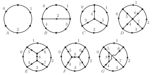
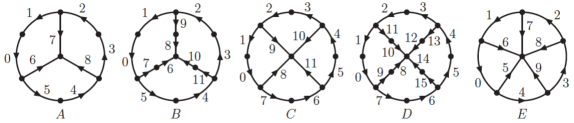
It has been shown from classical Aguilera-Verdugo:2020kzc ; Ramirez-Uribe:2020hes and quantum Ramirez-Uribe:2021ubp computations that the number of causal configurations of the multiloop topologies depicted in Fig. 1 is about one half of the total number of possible states. In order to achieve a succesful applicability of the quantum algorithm, there are two actions that can be undertaken. As a first option, we can halve the number of causal solutions to be queried by considering configurations with an edge fixed in one state. This can be done by either fixing a qubit in the oracle’s marker Ramirez-Uribe:2021ubp or excluding it from the circuit assuming that the qubit state is given. Halving the solutions to be queried is viable due to the fact that the objects of study are Feynman loop diagrams, which have the feature that given a causal solution the mirror state with all the momentum flows reversed is also a causal solution. A second adjustment, just in case the scenario requires it, is to introduce an extra qubit Nielsen:2012yss to increase the number of total states without increasing the number of solutions.
Moving on to the implementation of the quantum algorithm, three registers are needed. The first register, , encodes the states of all edges. We define the Boolean functions
| (5) |
where labels the set of edges depending on the same linear combination of loop momenta. The bar in denotes that the qubit states in this set are inverted with XNOT gates, . The number of edges in the set is denoted by and the total number of edges in the corresponding multiloop topology is . The second register required, , collects the causal conditions in eloop clauses. The last register, , stores the validation of the causal solutions in what is known as the oracle’s marker.
The algorithm takes as a first step the initialisation of all the quantum registers. The register encoding the edges’ states, , is initialised in a uniform superposition by applying Hadamard gates to each of its qubits, . For the eloop clauses, the qubits in the register are initialised to by the application of Pauli-X gates, . The oracle’s marker qubit, , is initialised to one of the Bell states by applying .
Following to the construction of the oracle, it is important to recall that causal configurations are identified as DAG configurations, therefore, the eloop clauses are established to suppress directed cyclic configurations. The eloop clauses are implemented through the application of multicontrolled Toffoli gates and XNOT gates that validate whether a configuration is cyclic or acyclic. To provide a convenient notation, we define the multicontrolled Toffoli operation based on Boolean clauses by
| (6) |
and
| (7) |
where the capital contains the set of edges generating the cyclic configuration involving the subloop . Both conditions in Eq. (6) select the same subloop but with opposite edge directions. The composite condition in Eq. (7) embraces both directions of the given subloop associated to . Let us recall that the eloop clause register is initialised to , therefore, applying one of the conditions in Eqs. (6) and (7) unmarks a noncausal configuration from .
The number of eloop clauses depends on the number of subloops needed to validate. An important aspect to consider relating eloop clauses is whether or not the set involves a fixed qubit, that is, a qubit in a definite state or . If the eloop clause condition does not involve a fixed qubit, we apply Eq. (7), which considers two multicontrolled Toffoli gates to validate both directions. The validation of both directions is stored in a single qubit , due to the fact that both configurations are mutually exclusive, i.e., applying one multicontrolled Toffoli gate do not overlap over the second one. In the case that the eloop clause involves a fixed qubit, the condition to prove involves only one direction, explicitly, only one of the two Boolean conditions given in Eq. (6) is tested.
After the initialisation of the registers and setting all the eloop clauses, the oracle operator is given by
| (8) |
where , and is the edge whose state is fixed. The procedure continues by performing the oracle operations in inverse order to restore every qubit but to its initial state. At this point we are ready to apply the diffusion operator, , to the register . The diffusion operator implemented is the one described in the IBM Qiskit website 111http://qiskit.org/.
The quantum algorithm presented in this paper has the advantage that the quantum circuit depth depends just on the number of eloop clauses and not on the number of edges per set, whereas the quantum circuit depth of the quantum algorithm using binary clauses Ramirez-Uribe:2021ubp increases when additional edges per set are considered.
Let us recall that the quantum circuit depth Depth:5769 is defined as the integer number of gates that need to be executed along the longest path of the circuit from input to output, moving forward in time along qubit wires. The input is understood as the preparation of the qubits and the output as the measurement gate. The quantum circuit depth is computed through the Qiskit routine, QuantumCircuit.depth()222https://qiskit-test.readthedocs.io. An important feature of the quantum circuit depth is the impact of quantum gates acting on no common qubits, allowing to perform them at the same time-step. On the other hand, if the gates act on at least one common qubit they have to be applied in different time-steps, increasing by one unit the quantum circuit depth. In the forthcoming sections we explore in a detailed way the performance of the algorithm by analysing the number of qubits needed for the implementation and the corresponding theoretical quantum circuit depth.
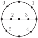

To illustrate the algorithm implementation, let us start with the two-loop topology with three sets of edges depicted in the top left of Fig. (2). We consider two edges per set to include three additional vertices representing external particles. Concretely, we have , , and , using the short hand notation . As previously stated, we start by preparing the three registers: set the register in a uniform superposition , the register initialised in the state and the oracle’s marker in the state as shown in the first time-step of the quantum circuit of Fig. (2) on the top right. The eloop clauses are given by
| (9) |
where , and . The eloops clauses in Eq. (3) are implemented by multicontrolled Toffoli gates taking as control the qubits in the set and as target the qubit with . Explicitly, and are implemented by a single multicontrolled Toffoli gate, whereas is implemented by two multicontrolled Toffoli gates.
For the oracle’s marker, another multicontrolled Toffoli gate is used. For this case we achieve an initial mixing angle of (see Table. 1) by fixing the qubit . The multicontrolled Toffoli gate implementing the oracle’s marker takes as control the qubits in the register and the qubit , and as target the qubit . After applying the oracle operations in reverse order, we apply the diffusion operator to the register . Table. 1 shows the results of the two quantum circuits in Fig. (2), exhibiting a clear improvement, going from to total number of qubits for implementation, and from to quantum depth.
| Fig. | eloops (edges) | Qubits | ||||
|---|---|---|---|---|---|---|
| 2 | two () |
4 Efficiency assessment
In this section we assess the efficiency of the current quantum algorithm by comparing the implementation results with the quantum algorithm and the multiloop topologies analysed in Ref. Ramirez-Uribe:2021ubp . These multiloop topologies are depicted in Fig. 1 considering one edge in each set. The results are summarised in Table 2 which displays the number of qubits required for the implementation, the theoretical quantum circuit depth, the related mixing angle and the number of causal configurations.
| Fig. | eloops (edges) | Qubits | ||||
|---|---|---|---|---|---|---|
| 1A | one () | |||||
| 1B | two () | |||||
| 1C | three () | |||||
| 1D | four(c) () | |||||
| 1E, 1F | four(t,s) () | |||||
| 1G | four(u) () |
The columns of total number of qubits and quantum circuit depth have two numbers: the first one gives the data on the current approach and, the second one the information of the algorithm using binary clauses. The remaining columns are: the initial mixing angle, an indicator for the appropriate selection of the iteration number and the number of causal states found by the algorithm. From Table 2, we observe that in all cases the initial mixing angle is close to , suggesting the application of one iteration only; from the fifth column we have that the value of the mixing angle after the first iteration approaches to , the desired probability amplification; with .
Moving on to the number of qubits, the quantum algorithm proposed in this work lowers significantly the total number of qubits required for the implementation, going from a two qubits reduction in the case of one eloop with three vertices, to a remarkable fourteen qubits reduction in the -channel at four eloops. Regarding the theoretical quantum circuit depth, we notice that the new approach gives smaller values for every topology, with the only exception of the -channel, which is a nonplanar diagram. Delving in the -channel case, it is important to take into account that the values shown in Table 2 corresponds to a configuration with one edge per set. The scenario with additional edges per set does not change the quantum circuit depth of the proposed algorithm whereas the quantum circuit depth of the algorithm using binary clauses increases as additional edges per set are included. Therefore, the behaviour of the quantum circuit depth comparative between both algorithms changes when we start considering more than one-edge-per-set complex multiloop diagrams, giving to the new algorithm an important advantage.
![[Uncaptioned image]](/html/2404.03544/assets/x6.png)
![[Uncaptioned image]](/html/2404.03544/assets/x7.png)
Continuing with the analysis of the quantum circuit depth, we observe in Table 2 a non-intuitive result, the quantum circuit depth for the three-eloop diagram is greater than the quantum circuit depth for the four-eloop diagram with one four-particle interaction vertex (also called N3MLT in Ref. Ramirez-Uribe:2020hes ). To better understand this behaviour we compare the eloop clauses needed for the implementation of both topologies to contrast the presence of multicontrolled Toffoli gates acting on noncommon qubits along the circuits. The eloop clauses required for the three-eloop topology are
| (10) |
and for the four-eloop topology are
| (11) | ||||||
For the three-eloop topology, the eloop clauses in Eq. (4) are translated to the quantum circuit into six multicontrolled Toffoli gates and their required CNOT gates. The clauses and validate only one direction of the subeloop, requiring a single multicontrolled Toffoli clause, while and test the subeloop in both directions, needing two multicontrolled Toffoli clauses each. In this case, we have all the Toffoli gates acting in at least one common edge, therefore, they have to be applied in different time-steps.
Regarding the four-eloop case, the eloop clauses in Eq. 4 are implemented into the quantum circuit with eight multicontrolled Toffoli gates together with the corresponding CNOT gates; and need a single multicontrolled Toffoli clause, whereas , and require two multicontrolled Toffoli clauses each. The edge configuration of this topology generates several multicontrolled Toffoli gates acting on noncommon qubits allowing to perform some of them at the same time-step.
An important feature of multicontrolled Toffoli gates to be discussed is transpilation. The transpilation process consists of compiling a given quantum circuit to match the specific topology and native gate set of a particular quantum device hardware, as well as its optimization in order to run on the noisy intermediate scale quantum (NISQ) era computers. In the quantum circuit model, the high level quantum circuits are built with unitary operators that are implemented as quantum gates. However, when running them on a real quantum hardware, they must undergo the decomposition of the unitary quantum gates into the native gate set of the target quantum device, and optimize them to reduce the noise effects on the results output.
We illustrate the impact on the quantum circuit depth for the transpilation of a Toffoli gate. The target device is ibmq_belem which has a set of native gates consisting of , , , , CNOT and a reset gate. The Toffoli gate in Fig. (4a) has a theoretical quantum depth of 1 while its transpilation process, Fig. (4b) results in a larger quantum depth of 19. We can see that for each Toffoli gate in the quantum circuit transpilation is costly increasing the quantum depth considerably. Therefore, this has an appreciable impact on the quantum noise and gate errors.
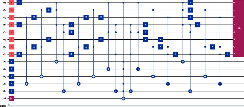
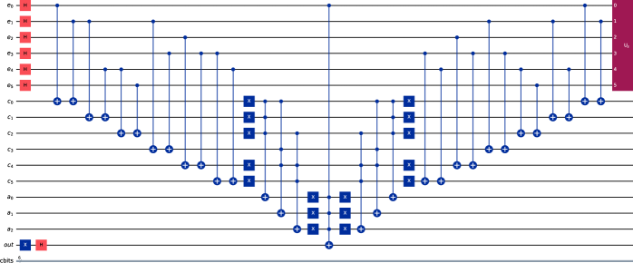
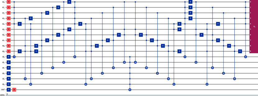
For example, the four-eloop topology with eight edges is implemented with the quantum circuit of Fig. (5) and requires fourteen qubits, while the binary-clause approach requires twenty five qubits. The transpilation process for the multicontrolled-Toffoli approach requires about 900 native gates on the ibmq_melbourne quantum device while with the binary-clause approach grows to around 1600 native gates in the ibmq_manila quantum device.
5 Multiloop topologies with multiple number of edges in each set
| eloops | Total Qubits | ||
|---|---|---|---|
| three | or | to | to |
| four(c,t,s,u) | or | to | to |
| five(c) | or | to |
In the previous section, we have shown a significant reduction on the total number of qubits required for the implementation of the quantum algorithm proposed in this work. This improvement allows to explore more complex topologies than those affordable with the algorithm presented in Ref. Ramirez-Uribe:2021ubp . In this section, we inquire into the implementation of the proposed algorithm to three-, four- and five-eloop topologies; the number of qubits required for an arbitrary number of edges per set is shown in Table 3. The particular cases presented are shown in Fig. 6; the number of eloop clauses to test in the oracle operator, the total number of qubits needed for the implementation, the quantum circuit depth and the mixing angle are summarised in Table 4.
5.1 Three eloops with nine and twelve edges
At three eloops, we work with the selected multiloop topologies shown in Figs. 6A and 6B. The first topolology (Fig. 6A) considers two edges in the external sets and one edge in the internal sets, and the Boolean functions are given by,
| (12) |
It requires the four eloop clauses in Eq. (4).
For the second topology (Fig. 6B), we take two edges in all the sets, and the Boolean functions are given by,
| (13) |
It requires in addition to the eloop clauses in Eq. (4), the following eloop clauses to test acyclicity over four sets of edges
| (14) | ||||||
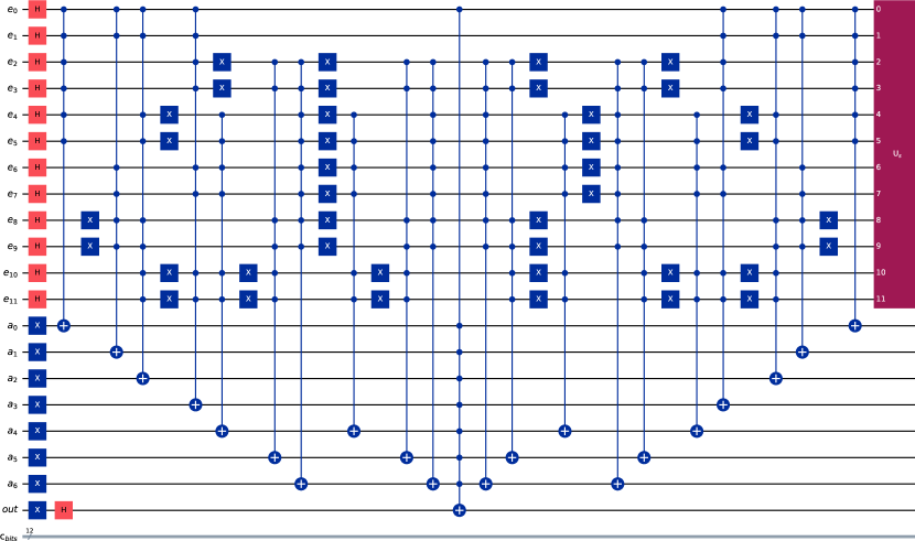
The total number of qubits required for the algorithm implementation of the configurations in Eq. (12) and Eq. (13) is fourteen and twenty one respectively, and the quantum circuit depth results in eighteen and thirty two, respectively. In comparison with the binary-clause approach, these configurations require twenty five and thirty six qubits, respectively; the latter exceeding the number of qubits available of current simulators. The quantum circuit depth for three eloops with nine edges is thirty two. The quantum circuit implemented for the configuration in Eq. (13) is shown in Fig. 7.
Regarding the eloop clauses, we have observed that the topology considering multiple edges located exclusively in the external sets do not enlarge the minimum number of clauses to test, whereas including two edges in every set requires to consider the three subloops involving four sets of edges.
5.2 Four eloops with twelve and sixteen edges
The four-eloop complexity examples to analyze are those depicted in Figs. 6C and 6D. The first topology (Fig. 6C) considers two edges in the external sets and one edge in the internal sets, and are given by
| (15) |
The second topology (Fig. 6D), consists in two edges in every set,
| (16) |
The complete set of clauses for the four-eloop topology of Fig. 6D, together with the clauses from Eq. (4) are given by
| (17) |
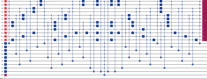
The implementation of the algorithm for these cases requires a total number of eighteen and thirty qubits respectively; the quantum circuit depth is sixteen and fourty six. The quantum circuit implemented for the topology configuration in Eq. (15) is shown in Fig. 8.
The topology associated to Eq. (16) requires thirty qubits which is within the capacities of Qiskit, nevertheless the number of shots needed to select all the causal configurations is beyond the Qiskit simulator capacities. Similar to the previous cases of three eloops, the topology associated to Eq. (15) do not need to test additional eloop clauses besides the minimum requirement. For the topology configuration in Eq. (16) with two edges in all the sets, it is necessary to check clauses with two and three subloops or equivalently, with four and five sets of edges, giving a total of thirteen eloop clauses for all the causal configurations.
| Fig. | eloops(edges) | |||||||||
|---|---|---|---|---|---|---|---|---|---|---|
| 6A | three () | |||||||||
| 6B | three() | |||||||||
| 6C | four(c)() | |||||||||
| 6D | four(c)() | |||||||||
| 6E | five(c)() |
5.3 Five eloops with ten egdes
The last topology we implement is a five-eloop case with a single edge per set , Fig. 6E. The clauses to validate are composed by
| (18) |
The output from the algorithm gives an angle with a single iteration , without the need of fixing a qubit from the register . This means that the probability of search success is close to one, , finding all the causal states out of the total states. Note that in this case we need to test every clause in both directions. With respect of the requirements for building the quantum circuit, we need 17 qubits to construct the corresponding quantum circuit (Fig. 9), and the quantum circuit depth is equal to 42.
6 Conclusions
We have presented an improved quantum algorithm for the identification of causal configurations for multiloop Feynman diagrams, which is equivalent to querry DAG configurations of undirected graphs in graph theory. The approach presented in this paper construct the oracle operator through multicontrolled Toffoli gates and XNOT gates only, allowing to reduce the total number of qubits required significantly. Additionaly, the quantum circuit depth do not increase by adding extra edges per set, it depends exclusively on the eloop clauses. Due to the lowering on the number of qubits needed, it was possible to explore more complex multiloop topologies through the IBM Quantum platform, in particular, we explicitly implemented the three eloops with six and nine vertices, the four eloops with twelve and sixteen vertices, and the five eloops with five point interaction with ten edges, successfully identifying their causal configurations.
Acknowledgements
We are very grateful to Fundación Centro Tecnológico de la Información y la Comunicación (CTIC) for granting us access to their simulator Quantum Testbed (QUTE). We thank also access to IBMQ. This work is supported by the Spanish Government (Agencia Estatal de Investigación MCIN/AEI/ 10.13039/501100011033) Grant No. PID2020-114473GB-I00, and Generalitat Valenciana Grant No. PROMETEO/2021/071 and ASFAE/2022/009 (Planes Complementarios de I+D+i, NextGenerationEU). This work is also supported by the Ministry of Economic Affairs and Digital Transformation of the Spanish Government and NextGenerationEU through the Quantum Spain project, and by CSIC Interdisciplinary Thematic Platform (PTI+) on Quantum Technologies (PTI-QTEP+). SRU acknowledges support from CONAHCyT through Project No. 320856 (Paradigmas y Controversias de la Ciencia 2022), Ciencia de Frontera 2021-2042 and Sistema Nacional de Investigadores; AERO from the Spanish Government (PRE2018-085925).
References
- (1) R. P. Feynman, Simulating physics with computers, Int. J. Theor. Phys. 21 (1982) 467–488.
- (2) T. S. Humble, G. N. Perdue and M. J. Savage, Snowmass Computational Frontier: Topical Group Report on Quantum Computing, 2209.06786.
- (3) G. Rodrigo, Quantum Algorithms in Particle Physics, Acta Phys. Polon. Supp. 17 (2024) 2–A14, [2401.16208].
- (4) S. P. Jordan, K. S. M. Lee and J. Preskill, Quantum Algorithms for Quantum Field Theories, Science 336 (2012) 1130–1133, [1111.3633].
- (5) M. C. Bañuls et al., Simulating Lattice Gauge Theories within Quantum Technologies, Eur. Phys. J. D 74 (2020) 165, [1911.00003].
- (6) E. Zohar, J. I. Cirac and B. Reznik, Quantum Simulations of Lattice Gauge Theories using Ultracold Atoms in Optical Lattices, Rept. Prog. Phys. 79 (2016) 014401, [1503.02312].
- (7) T. Byrnes and Y. Yamamoto, Simulating lattice gauge theories on a quantum computer, Phys. Rev. A 73 (2006) 022328, [quant-ph/0510027].
- (8) D. Magano et al., Quantum speedup for track reconstruction in particle accelerators, Phys. Rev. D 105 (2022) 076012, [2104.11583].
- (9) P. Duckett, G. Facini, M. Jastrzebski, S. Malik, T. Scanlon and S. Rettie, Reconstructing charged particle track segments with a quantum-enhanced support vector machine, Phys. Rev. D 109 (2024) 052002, [2212.07279].
- (10) T. Schwägerl, C. Issever, K. Jansen, T. J. Khoo, S. Kühn, C. Tüysüz et al., Particle track reconstruction with noisy intermediate-scale quantum computers, 2303.13249.
- (11) A. Y. Wei, P. Naik, A. W. Harrow and J. Thaler, Quantum Algorithms for Jet Clustering, Phys. Rev. D 101 (2020) 094015, [1908.08949].
- (12) D. Pires, Y. Omar and J. a. Seixas, Adiabatic quantum algorithm for multijet clustering in high energy physics, Phys. Lett. B 843 (2023) 138000, [2012.14514].
- (13) J. J. M. de Lejarza, L. Cieri and G. Rodrigo, Quantum clustering and jet reconstruction at the LHC, Phys. Rev. D 106 (2022) 036021, [2204.06496].
- (14) J. J. M. de Lejarza, L. Cieri and G. Rodrigo, Quantum jet clustering with LHC simulated data, PoS ICHEP2022 (2022) 241, [2209.08914].
- (15) J. a. Barata and C. A. Salgado, A quantum strategy to compute the jet quenching parameter , Eur. Phys. J. C 81 (2021) 862, [2104.04661].
- (16) J. a. Barata, X. Du, M. Li, W. Qian and C. A. Salgado, Medium induced jet broadening in a quantum computer, Phys. Rev. D 106 (2022) 074013, [2208.06750].
- (17) J. a. Barata, X. Du, M. Li, W. Qian and C. A. Salgado, Quantum simulation of in-medium QCD jets: Momentum broadening, gluon production, and entropy growth, Phys. Rev. D 108 (2023) 056023, [2307.01792].
- (18) C. W. Bauer, W. A. de Jong, B. Nachman and D. Provasoli, Quantum Algorithm for High Energy Physics Simulations, Phys. Rev. Lett. 126 (2021) 062001, [1904.03196].
- (19) C. W. Bauer, M. Freytsis and B. Nachman, Simulating Collider Physics on Quantum Computers Using Effective Field Theories, Phys. Rev. Lett. 127 (2021) 212001, [2102.05044].
- (20) K. Bepari, S. Malik, M. Spannowsky and S. Williams, Towards a quantum computing algorithm for helicity amplitudes and parton showers, Phys. Rev. D 103 (2021) 076020, [2010.00046].
- (21) K. Bepari, S. Malik, M. Spannowsky and S. Williams, Quantum walk approach to simulating parton showers, Phys. Rev. D 106 (2022) 056002, [2109.13975].
- (22) A. Pérez-Salinas, J. Cruz-Martinez, A. A. Alhajri and S. Carrazza, Determining the proton content with a quantum computer, Phys. Rev. D 103 (2021) 034027, [2011.13934].
- (23) J. M. Cruz-Martinez, M. Robbiati and S. Carrazza, Multi-variable integration with a variational quantum circuit, 2308.05657.
- (24) H. A. Chawdhry and M. Pellen, Quantum simulation of colour in perturbative quantum chromodynamics, SciPost Phys. 15 (2023) 205, [2303.04818].
- (25) W. A. De Jong, M. Metcalf, J. Mulligan, M. Płoskoń, F. Ringer and X. Yao, Quantum simulation of open quantum systems in heavy-ion collisions, Phys. Rev. D 104 (2021) 051501, [2010.03571].
- (26) W. Guan, G. Perdue, A. Pesah, M. Schuld, K. Terashi, S. Vallecorsa et al., Quantum Machine Learning in High Energy Physics, Mach. Learn. Sci. Tech. 2 (2021) 011003, [2005.08582].
- (27) S. L. Wu et al., Application of quantum machine learning using the quantum variational classifier method to high energy physics analysis at the LHC on IBM quantum computer simulator and hardware with 10 qubits, J. Phys. G 48 (2021) 125003, [2012.11560].
- (28) T. Felser, M. Trenti, L. Sestini, A. Gianelle, D. Zuliani, D. Lucchesi et al., Quantum-inspired machine learning on high-energy physics data, npj Quantum Inf. 7 (2021) 111, [2004.13747].
- (29) S. Herbert, Quantum Monte Carlo Integration: The Full Advantage in Minimal Circuit Depth, Quantum 6 (2022) 823, [2105.09100].
- (30) G. Agliardi, M. Grossi, M. Pellen and E. Prati, Quantum integration of elementary particle processes, Phys. Lett. B 832 (2022) 137228, [2201.01547].
- (31) J. J. M. de Lejarza, M. Grossi, L. Cieri and G. Rodrigo, Quantum Fourier Iterative Amplitude Estimation, in 2023 International Conference on Quantum Computing and Engineering, IEEE, 5, 2023. 2305.01686. DOI.
- (32) J. J. M. de Lejarza, L. Cieri, M. Grossi, S. Vallecorsa and G. Rodrigo, Loop Feynman integration on a quantum computer, 2401.03023.
- (33) S. Ramírez-Uribe, A. E. Rentería-Olivo, G. Rodrigo, G. F. R. Sborlini and L. Vale Silva, Quantum algorithm for Feynman loop integrals, JHEP 05 (2022) 100, [2105.08703].
- (34) G. Clemente, A. Crippa, K. Jansen, S. Ramírez-Uribe, A. E. Rentería-Olivo, G. Rodrigo et al., Variational quantum eigensolver for causal loop Feynman diagrams and directed acyclic graphs, Phys. Rev. D 108 (2023) 096035, [2210.13240].
- (35) R. K. Ellis et al., Physics Briefing Book: Input for the European Strategy for Particle Physics Update 2020, 1910.11775.
- (36) F. Gianotti et al., Physics potential and experimental challenges of the LHC luminosity upgrade, Eur. Phys. J. C 39 (2005) 293–333, [hep-ph/0204087].
- (37) FCC collaboration, A. Abada et al., FCC Physics Opportunities: Future Circular Collider Conceptual Design Report Volume 1, Eur. Phys. J. C 79 (2019) 474.
- (38) ILC collaboration, G. Aarons et al., International Linear Collider Reference Design Report Volume 2: Physics at the ILC, 0709.1893.
- (39) CLIC, CLICdp collaboration, The Compact Linear e+e- Collider (CLIC): Physics Potential, 1812.07986.
- (40) CEPC Study Group collaboration, M. Dong et al., CEPC Conceptual Design Report: Volume 2 - Physics & Detector, 1811.10545.
- (41) G. Heinrich, Collider Physics at the Precision Frontier, Phys. Rept. 922 (2021) 1–69, [2009.00516].
- (42) S. Catani, T. Gleisberg, F. Krauss, G. Rodrigo and J.-C. Winter, From loops to trees by-passing Feynman’s theorem, JHEP 09 (2008) 065, [0804.3170].
- (43) I. Bierenbaum, S. Catani, P. Draggiotis and G. Rodrigo, A Tree-Loop Duality Relation at Two Loops and Beyond, JHEP 10 (2010) 073, [1007.0194].
- (44) I. Bierenbaum, S. Buchta, P. Draggiotis, I. Malamos and G. Rodrigo, Tree-Loop Duality Relation beyond simple poles, JHEP 03 (2013) 025, [1211.5048].
- (45) E. T. Tomboulis, Causality and Unitarity via the Tree-Loop Duality Relation, JHEP 05 (2017) 148, [1701.07052].
- (46) R. Runkel, Z. Szőr, J. P. Vesga and S. Weinzierl, Causality and loop-tree duality at higher loops, Phys. Rev. Lett. 122 (2019) 111603, [1902.02135].
- (47) Z. Capatti, V. Hirschi, D. Kermanschah and B. Ruijl, Loop-Tree Duality for Multiloop Numerical Integration, Phys. Rev. Lett. 123 (2019) 151602, [1906.06138].
- (48) S. Buchta, G. Chachamis, P. Draggiotis, I. Malamos and G. Rodrigo, On the singular behaviour of scattering amplitudes in quantum field theory, JHEP 11 (2014) 014, [1405.7850].
- (49) R. J. Hernandez-Pinto, G. F. R. Sborlini and G. Rodrigo, Towards gauge theories in four dimensions, JHEP 02 (2016) 044, [1506.04617].
- (50) J. L. Jurado, G. Rodrigo and W. J. Torres Bobadilla, From Jacobi off-shell currents to integral relations, JHEP 12 (2017) 122, [1710.11010].
- (51) F. Driencourt-Mangin, G. Rodrigo, G. F. R. Sborlini and W. J. Torres Bobadilla, Interplay between the loop-tree duality and helicity amplitudes, Phys. Rev. D 105 (2022) 016012, [1911.11125].
- (52) J. J. Aguilera-Verdugo, F. Driencourt-Mangin, J. Plenter, S. Ramírez-Uribe, G. Rodrigo, G. F. R. Sborlini et al., Causality, unitarity thresholds, anomalous thresholds and infrared singularities from the loop-tree duality at higher orders, JHEP 12 (2019) 163, [1904.08389].
- (53) S. Buchta, G. Chachamis, P. Draggiotis and G. Rodrigo, Numerical implementation of the loop–tree duality method, Eur. Phys. J. C 77 (2017) 274, [1510.00187].
- (54) G. F. R. Sborlini, F. Driencourt-Mangin, R. Hernandez-Pinto and G. Rodrigo, Four-dimensional unsubtraction from the loop-tree duality, JHEP 08 (2016) 160, [1604.06699].
- (55) G. F. R. Sborlini, F. Driencourt-Mangin and G. Rodrigo, Four-dimensional unsubtraction with massive particles, JHEP 10 (2016) 162, [1608.01584].
- (56) F. Driencourt-Mangin, G. Rodrigo and G. F. R. Sborlini, Universal dual amplitudes and asymptotic expansions for and in four dimensions, Eur. Phys. J. C 78 (2018) 231, [1702.07581].
- (57) F. Driencourt-Mangin, G. Rodrigo, G. F. R. Sborlini and W. J. Torres Bobadilla, Universal four-dimensional representation of at two loops through the Loop-Tree Duality, JHEP 02 (2019) 143, [1901.09853].
- (58) Z. Capatti, V. Hirschi, D. Kermanschah, A. Pelloni and B. Ruijl, Numerical Loop-Tree Duality: contour deformation and subtraction, JHEP 04 (2020) 096, [1912.09291].
- (59) J. Plenter, Asymptotic Expansions Through the Loop-Tree Duality, Acta Phys. Polon. B 50 (2019) 1983–1992.
- (60) R. M. Prisco and F. Tramontano, Dual subtractions, JHEP 06 (2021) 089, [2012.05012].
- (61) J. Plenter and G. Rodrigo, Asymptotic expansions through the loop-tree duality, Eur. Phys. J. C 81 (2021) 320, [2005.02119].
- (62) R. Runkel, Z. Szőr, J. P. Vesga and S. Weinzierl, Integrands of loop amplitudes within loop-tree duality, Phys. Rev. D 101 (2020) 116014, [1906.02218].
- (63) J. J. Aguilera-Verdugo, F. Driencourt-Mangin, R. J. Hernández-Pinto, J. Plenter, S. Ramirez-Uribe, A. E. Renteria Olivo et al., Open Loop Amplitudes and Causality to All Orders and Powers from the Loop-Tree Duality, Phys. Rev. Lett. 124 (2020) 211602, [2001.03564].
- (64) J. J. Aguilera-Verdugo, R. J. Hernández-Pinto, S. Ramírez-Uribe, A. E. Rentería-Olivo, G. Rodrigo, G. F. R. Sborlini et al., Manifestly Causal Scattering Amplitudes, Snowmass LoI (August 2020) .
- (65) J. J. Aguilera-Verdugo, R. J. Hernandez-Pinto, G. Rodrigo, G. F. R. Sborlini and W. J. Torres Bobadilla, Causal representation of multi-loop Feynman integrands within the loop-tree duality, JHEP 01 (2021) 069, [2006.11217].
- (66) J. Jesús Aguilera-Verdugo, R. J. Hernández-Pinto, G. Rodrigo, G. F. R. Sborlini and W. J. Torres Bobadilla, Mathematical properties of nested residues and their application to multi-loop scattering amplitudes, JHEP 02 (2021) 112, [2010.12971].
- (67) S. Ramírez-Uribe, R. J. Hernández-Pinto, G. Rodrigo, G. F. R. Sborlini and W. J. Torres Bobadilla, Universal opening of four-loop scattering amplitudes to trees, JHEP 04 (2021) 129, [2006.13818].
- (68) G. F. R. Sborlini, Geometrical approach to causality in multiloop amplitudes, Phys. Rev. D 104 (2021) 036014, [2102.05062].
- (69) W. J. Torres Bobadilla, Loop-tree duality from vertices and edges, JHEP 04 (2021) 183, [2102.05048].
- (70) W. J. T. Bobadilla, Lotty – The loop-tree duality automation, Eur. Phys. J. C 81 (2021) 514, [2103.09237].
- (71) J. de Jesús Aguilera-Verdugo et al., A Stroll through the Loop-Tree Duality, Symmetry 13 (2021) 1029, [2104.14621].
- (72) J. Rios-Sanchez and G. Sborlini, Towards multiloop local renormalization within Causal Loop-Tree Duality, 2402.13995.
- (73) S. Ramírez-Uribe, A. E. Rentería-Olivo, G. Rodrigo and G. F. R. Sborlini, Method for generating in a random order directed acyclic graph (DAG) configurations of a given graph in a quantum computing device , European patent application EP24382213 (28 February 2024) .
- (74) C. G. Bollini and J. J. Giambiagi, Dimensional Renormalization: The Number of Dimensions as a Regularizing Parameter, Nuovo Cim. B 12 (1972) 20–26.
- (75) G. ’t Hooft and M. J. G. Veltman, Regularization and Renormalization of Gauge Fields, Nucl. Phys. B 44 (1972) 189–213.
- (76) M. Boyer, G. Brassard, P. Hoeyer and A. Tapp, Tight bounds on quantum searching, Fortsch. Phys. 46 (1998) 493–506, [quant-ph/9605034].
- (77) L. K. Grover, Quantum mechanics helps in searching for a needle in a haystack, Phys. Rev. Lett. 79 (1997) 325–328, [quant-ph/9706033].
- (78) M. A. Nielsen and I. L. Chuang, Quantum Computation and Quantum Information, Cambridge University Press (6, 2012) .
- (79) https://quantumcomputing.stackexchange.com/questions/5769/how-to-calculate-circuit-depth-properly, 2020.