Early warning systems for financial markets
of emerging economies††thanks: An early version of the paper was presented at iCEBA23 and META23 and the authors are grateful for feedback received from the participants. Prokhorov’s research was supported by a grant from the Russian Science Foundation.
Abstract
We develop and apply a new online early warning system (EWS) for what is known in machine learning as concept drift, in economics as a regime shift and in statistics as a change point. The system goes beyond linearity assumed in many conventional methods, and is robust to heavy tails and tail-dependence in the data, making it particularly suitable for emerging markets. The key component is an effective change-point detection mechanism for conditional entropy of the data, rather than for a particular indicator of interest. Combined with recent advances in machine learning methods for high-dimensional random forests, the mechanism is capable of finding significant shifts in information transfer between interdependent time series when traditional methods fail. We explore when this happens using simulations and we provide illustrations by applying the method to Uzbekistan’s commodity and equity markets as well as to Russia’s equity market in 2021-2023.
Keywords: early warning, copula, local random forest, machine learning, Shiryaev-Roberts statistic, spillover effects
1 Introduction
Financial markets of emerging economies are characterized by unusually high volatility, structural breaks, non-linear dependence, asymmetry and strong correlation in extremes also known as tail-dependence. There is evidence that these stylized facts are particularly pronounced in emerging markets (see, e.g., Chaudhuri and Wu, 2003; Chen and Ibragimov, 2019). Moreover, modern financial markets generally have a complicated structure of information flows often represented by various global and local spillover and contagion effects, involving emerging markets and manifesting themselves with significant lags and frictions in information transfer (see, e.g., Zhao et al., 2022; Khalfaoui et al., 2023; Ahmad et al., 2018). In this setting, rapid and reliable detection of shifts in information channels at work in emerging markets is key to ensuring stability of the markets, effective economic policy and prevention of financial contagion (see, e.g., Neaime, 2016; Smimou and Khallouli, 2015; Yang et al., 2023).
From the statistical perspective, the area that develops principled ways of constructing early warning systems (EWS) which react to changes in a stochastic process with the shortest delay, is known as change-point detection. This literature tracks back to Shiryaev (1961, 1963) and Roberts (1966), among others, and has by now accummulated an impressive set of optimality results (see, e.g., Chen, 2019; Chu and Chen, 2019; Pergamenchtchikov and Tartakovsky, 2018, 2019). Importantly, various versions of the so called Shiryaev-Roberts (SR) statistic have been shown to be optimal in terms of minimizing the detection delay as the probability of false alarm approaches zero, for a wide range of stochastic processes including autocorrelated time series of financial returns with unknown pre- and post-change distribution. This has spurred the development of online financial surveillance systems based on the SR statistic where “online” means real-time (see, e.g., Pepelyshev and Polunchenko, 2017).
The use of these methodologies in economic applications and, in particular, for emerging markets has been lagging. In econometrics, most of what is known as structural breaks methodology has been “offline,” that is, it uses historical time series to find regime shifts (see, e.g., Hamilton, 2016; Bai and Perron, 1998, 2003). The focus has been on obtaining consistent tests for the number and location of regime shifts in the available data, rather than on sequential monitoring for change points. The conventional econometric methodology often assumes the number of regime shifts to be known or to be within a fixed region. Comparisons of performance between online and offline methods requires re-designing the offline methods to make them applicable in an online environment for which they were not designed. Therefore, there is little guidance in the literature on choosing between these methods. Moreover, traditionally economics has focused on linear models of information transfer, represented in such concepts and models as Granger (1969) causality, vector autoregression (VAR) and dynamic conditional covariance (DCC) models, which use primarily parametric specifications and may suffer from large misspecification biases.
Meanwhile, the field of machine learning has seen remarkable advances in areas related to the task of change-point detection. Known as concept drift or data drift detection, this field of machine learning recognizes that the conditional distribution of target variable given explanatory variables may change, drastically affecting predictive capacity of a machine learning engine trained on data from that distribution (see, e.g., Hoens, 2012; Chen et al., 2022). This brings to the fore the recent successes of advanced machine learning methods such as random forests and artificial neural networks in estimating flexible nonparametric conditional distributions with high dimensions of the conditioning set (see, e.g., Breiman, 2001; Pospisil and Lee, 2018; Friedberg et al., 2021).
Much relevant work is now happening in the intersection of machine learning and statistics. For example, Barros (2018) develop a statistical estimator for concept drift detection based on Wilcoxon rank sum test to investigate the stationarity of the concept. Baidari and Nagaraj (2021) apply the Bhattacharyya (1943) test to online concept drift detection. Wang (2023) used shifts in the estimates covariance matrix to detect change points which restricts the attention to linear shifts; Ditzler and Polikar (2011) used shifts in the target variable distribution over time more generally. Bifet and Gavalda (2007) effectively did the same but focused on developing a method of adaptive windowing (ADWIN) for high-frequency data streams monitoring. Raab et al. (2020) extended ADWIN to use the Kolmogorov-Smirnov statistic (KSWIN) and provided a more stable and precise estimation. Tajeuna et al. (2023) develop method for finding regime shifts in multivariate time series via analyzing the co-evolving time series representation called mapping grid, while Guo et al. (2022) and Alanqary et al. (2021) develop new ways for measuring changes in statistical properties of multivariate distributions. Empirical economics is yet to benefit from these methodological advances.
The goal of this paper is to advance the early warning methodology by combining these advances in statistics and machine learning with application in economics and finance, in particular in settings with highly volatile and tail-dependent data. Specifically, we design a new version of the change-point detection methodology based on conditional entropy. The novelty here is that information transfer is not restricted to be linear and incorporates regime shifts in any feature of the distribution, not only the mean or the variance. In fact, the mean and variance of the underlying series may not even be well defined. The EWS we design is sensitive to any shift in the conditional entropy based on a local random forest estimator of a conditional density, which relates the present state of the target variable to the information in the explanatory variables not captured by the lags of the target variable. In this setup, we directly measure the amount of uncertainty that cannot be explained either by the lags of the target or by explanatory variables without restricting the relationships to be linear and parametric, or focusing on a specific feature of the target distribution.
As a starting point we take the conventional linear specification of the kind commonly used for Granger causality testing and convert it into a time series of conditional entropy estimates based on a sliding window of residuals from an autoregression (AR) of the target variable. This gives rise to an online sequential SR statistic. To our knowledge, the use of conditional entropy in the SR statistic is novel and of interest in its own right. Then, we develop extensions of this baseline setting to take advantage of the benefits provided by the random forest estimation and by fact that based the procedure on ranks of the data, rather than the data itself. This permits for non-linearity, tail-dependence and infinite moments as we now deal with the statistical copula which captures non-linear dependence present in the data even if the data is extremely heavy tailed. The simulations we present demonstrate that the new approach dominates application of the SR statistic directly to the target variable or the AR process residuals. They also outline the cases when using ranks permits to pick regime shifts that cannot be detected by the conventional SR statistic and when the other methods of change-point detection fail or perform suboptimally. The empirical section provides illustrations of use but is not aimed at providing meaningful macroeconomic interpretations of the uncovered information flows.
The paper proceeds as follows. Section 2 sets the stage by defining notation and concepts such as entropy, random forest estimation and change-point detection. Section 3 describes the baseline version of the proposed procedure. Section 4 describes extensions of the baseline method to better account for non-linearity and ranks. Numerous simulations are provided in Section 5, and Section 6 contains applications. Section 7 concludes. All the codes and data for this paper are available at https://github.com/kraevskiyAA/EWS_CondEnt
2 Preliminaries and related literature
2.1 Entropy and information transfer
Suppose we have a target time series and a history of explanatory variables available at time , , where each is a matrix containing explanatory variables (or their lags). As an example, to which we return in our empirical application, can be a composite stock index of an emerging market and can contain histories of commodity prices the country trades in. Our goal is to detect shifts in information transfer between the target and explanatory variables, causing an early warning for the state of the market described by the target variable. It is common to evaluate information transfer intensity from to by conditional entropy of given (see, e.g., Orlitsky, 2003) which can be written as follows:
| (1) |
where is the conditional density of given , is the joint density of , and is the marginal density of . The last equality follows from the definition of expectations and the law of interated expectations.
Fundamentally, the concept of entropy measures the uncertainty about given the information . In the context of signal transmission and unconditional distributions, Hartley (1928) is credited for observing that the information to be gained from outcomes each having a different probability can be defined as
This has become known as the Shannon entropy (Shannon, 1948). The higher this value, the higher is the uncertainty about the realizations.111A famous and straightforward example is a coin flip: the uncertainty is limited to two outcomes, head or tail. The information to be gained from a flip, known as a bit, is binary and can be defined by . Then, the information to be gained from flips is . The largest amount of uncertainty corresponds to uniformly distributed outcomes, i.e. the same for all . Eq. (1) can be viewed as a generalization of this concept to continuous conditional distributions, showing the average amount of information to be supplied before one can communicate the information in given that the other party knows the information in .
2.2 Nonparametrics and random forests
An important component of computing is estimation of the conditional density. A flexible way of estimating without making questionable distributional assumptions is to use the tools from nonparametric econometrics (see, e.g., Li and Racine, 2023). However, most of the standard methods will not work when the dimension of is even moderately large. This is known as the curse of dimensionality. Additionally, the nonparametric methods are known to perform poorly in the extremes of the distribution, which are of particular interest when dealing with data from emerging markets.
An alternative approach that has been gaining popularity but has not been explored in the context of entropy-based EWS is to use machine learning techniques. For example, Pospisil and Lee (2018) propose to use random forest for conditional density estimation (RFCDE). The estimator improves on a standard nonparametric method of kernel density esimation (KDE) by employing adaptive weights obtained using random forests of Breiman (2001). The main advantage here is that random forests break the curse of dimensionality by using random subsamples of the entire set of conditioning variables. This allows RFCDE to achieve consistent conditional density estimation with low computational costs and high accuracy.
It is then intuitive that a spike in evaluated using RFCDE over a sliding window should indicate an increase in uncertainty (a decrease in the information transfer from to ) and the remaining question is how to identify significant spikes.
2.3 Change-point detection
The change-point detection literature, going back at least 60 year (Shiryaev, 1961, 1963; Roberts, 1966), looks at an aggregated sequence of likelihood ratios based on the likelihood of a break at time versus the likelihood of no break, over a history of observations, where the densities before and after the change are known but the change point is not. There are important relaxations of the assumptions of known densities and operational methods that look at a sliding window of data rather than the entire history. However, this literature has not looked at the settings of entropy- or rank-based evaluation of information transfer with no knowledge of the true densities.
Define the Shiryaev-Roberts statistic as follows:
| (2) |
where are generic independent random variables or vectors, is the density of before the change and is the density of after the change. Then, it is easy to derive the recursive version
| (3) |
We use a version of the weighted SR statistics proposed by Tartakovsky and Spivak (2021). The procedure permits randomness in the drift of in the sense that at each the change may take one of values and the weighted statistic has the form
| (4) |
where is the value of when the difference between the mean of and the mean of is .222We use shifts in the mean with a fixed step equal to the range of data divided by m. This affords a much better performance in cases when distribution parameters are unknown. Other than that, the construction of the statistic is standard (see, e.g., Pepelyshev and Polunchenko, 2017).
An alarm will sound when exceeds a threshold value that controls the false alarm rate and, based on a series of important results, the SR procedure is optimal in the sense of minimizing the average detection delay (see, e.g., Polunchenko and Tartakovsky, 2010).
3 The new procedure: baseline version
The core of the new procedure is application of the Shiryaev-Roberts statistic to a sequence of entropy estimates of assessed on a moving window of length . The window length needs to be short enough so that the regime shift is noticeable but long enough not to pick noise (we use window lengths of 50 to 100 observations in practice). An EWS signal is triggered when evaluated using the process surpasses a threshold , indicating a significant shift in information transmission from to . In this section we discuss how we construct the sequence, statistic, and threshold.
We start by fitting an autoregressive model for the target variable on a moving window of length :
| (5) |
where we use the BIC to determine the optimal AR order . This gives the part of orthogonal to the history of the target variable, which is the unexpected component of we are interested in:
| (6) |
The AR(k) residuals capture any remaining news of the target variable and we wish to explore how the distribution of this variable changes depending on the explanatory variables . We wish to remain agnostic about the specific moment of the distribution that changed or the form of the distribution.
Then, we obtain the fitted value from the regresion of on lags of the explanatory variables contained in using the same moving window:
| (7) |
where is one of the available explanatory variables, lagged times, . Again, the optimal lag can be selected by BIC. Clearly, these two steps are equivalent to a one-step regression of on both its own history and history of the covariates. This would correspond to the familiar concept of Granger causality, which could be detected by a joint significance test on .
We go beyond the Granger causality and compute the conditional entropy of given . This recognizes the fact that change-point detection should be based on the conditional distribution rather than linear regression, thus accommodating more complex (than linear in mean) patterns of dependence.
Let denote the RFCDE of the conditional density of given obtained using the moving window of size . Let denote the set of ’s that fall into the window. Then, the estimator of aggregate information transfer over the window can be written as a sum of the entropy contributions for the values of that fall into the window:
| (8) |
We can approximate the summand integrals using stochastic or deterministic integral appoximation, e.g., Simpson’s rule which is a deterministic method. We are interested in early identification of spikes in as we move across time. Denote the sequence of entropy estimates over a sliding window of size as follows
We note that the step between the values of in the sequence can be larger than one time period but this delays detection while expediting computation. This is the time series to which we apply the SR statistic in the baseline version of our approach.
Algorithm 1 outlines the Shiryaev-Roberts procedure for entropy-based change-point detection described above. The algorithm uses several inputs besides the sequence of , namely, the set of shift values , the threshold and the smoothing parameters and . Although there is no strict rule for selecting the value of threshold , it is customary to consider two minimization criteria, namely, average detection delay (ADD) defined as and probability of false alarm (PFA) defined as , where is the actual moment of the change-point and is the moment of time it is detected.
Pergamenchtchikov and Tartakovsky (2018, 2019) show that the weighted SR procedure approximately minimizes ADD among all change-point detection procedures with a given PFA within a window of a fixed length for non-i.i.d. data, including autoregressions and conditional heteroskedasticity GARCH-type models. However, these quantities are generally unavailable to the researcher in practice, unless one deals with synthetic data and is able to generate it for a given constellation of these parameters. For instance, in Section 5 where we consider simulations, we are able to set by choosing the values of ADD and PFA via the numerous relationships derived in the literature (see, e.g., Tartakovsky, 2016).
Smoothing parameters and are used at the end of each iteration of Algorithm 1 in order to produce an exponential moving average update of the conditional expectation and variance of , balancing the past values and the new information. The natural value for is 0.5, reflecting equal weights on the old value of the mean and the current , while for the variance update, we choose , putting more weight on the estimate of from the previous period and thus dampening the variance update. Larger values result in smoother trajectories of the moments of .
4 Extensions to non-linear and rank-based estimation
The baseline procedure described in previous section uses a conditional density estimator of the AR process residuals given , where represents the linear span of the lagged explanatory variables in Eq. (7). This aligns with the traditional view of the Granger causality, which identifies information transfer by testing joint significance the lagged regressors in a linear autoregressive model. In the previous section, we extended the traditional approach by constructing a flexible, kernel-based estimator of and by applying the SR statistic to a moving window of entropy estimates obtained using . The goal here is to adapt the approach to the most flexible non-linear specification, recognizing the well documented presence of non-linearities in financial market data (see, e.g., Caporale et al., 2020)
4.1 Local linear forest
The univariate conditioning in substantially simplifies the task of nonparametric density estimation. The alternative of conditioning on the entire set of covariates separately, without obtaining , leads to a nonparametric estimator which suffers from a severe curse of dimensionality due to high dimensionality of , making the estimate very imprecise. The problem is further exacerbated by the trade-off between quick detection delay and accuracy of density estimation. It is well known in the change-point detection literature that if we increase the rolling window, making the density estimation more precise, the time before change-point detection increases. Thus, a multivariate nonparametric estimator either suffers from a curse of dimensionality or detects the change point with a suboptimal delay.
To overcome this issue without increasing the dimensionality of density estimation, we use a recently developed method of local linear forest (LLF) proposed by Friedberg et al. (2021). LLF constructs an estimate of the conditional mean achieving a faster convergence rate than traditional nonparametric estimators of the same dimensionality, and preventing the overfitting. The standard (non-local) random forest estimator (see, e.g., Breiman, 2001; Probst et al., 2019) is sensitive to hyperparameter selection and tends to overfit.
Therefore, our first extension of the baseline methodology is to use the flexible LLF estimator instead of the fitted value in constructing . The SR statistic is now based on a sequence of the new estimates of on a sliding window :
| (9) |
where . The rest of the methodology remains unchanged.
We note that both and permit non-linearity in the relationship of on because both use RFCDE to construct the conditional density of . The additional advantage of using the new estimates is that implies a non-linear conditional mean of in terms of , given lags of . Therefore, it aligns with the notion of non-linear Granger causality where Granger-causes if the nonparametric estimator is indistinguishable from a constant in each dimension of . Unfortunately, powerful statistical tests of this null hypothesis in a setting with many covariates in do not exist. The procedure we propose does not require such testing.
4.2 Copulas
Our second extension addresses the problem of heavy tails and tail-dependence, in addition to the problem of non-linearity. It is well documented that financial markets of emerging economies are characterized by asymmetric heavy-tailed distribution, which make application of standard econometric methods problematic (see, e.g., Chen and Ibragimov, 2019). As an alternative we follow the growing literature on copula-based estimation in finance (see, e.g., Ibragimov and Prokhorov, 2017) and re-formulate the problem of density estimation using ranks instead of actual values. It is important to note that for any set of random variables, their copula function contains all information about the dependence structure between the random variable as well as between any rank-preserving transformations of the random variables (see, e.g., Cherubini et al., 2011, for a survey of copula methods in finance). Therefore, if we use the copula instead of the original data distribution in the baseline method, the structure of information transfer will remain unchanged while the estimation is now over ranks and uses conditional copula density which is robust to heavy tails in the marginal distributions and is well defined even when moments of the original distributions may be infinite.
In the proposed modification, the baseline RFCDE estimator is replaced by the rank-based RFCDE estimator , where
where, as before, is the length of the sliding window over which we estimate the densities. The values of and are known as pseudo-observations; they are values between corresponding to the ranks of observations and , respectively, in the sliding window, divided by the number of observations in the window. The corresponding entropy estimates can be written as follows
| (10) |
where and can be interpreted as the conditional copula density of given . The remaining parts of the procedure are unchanged. We also considered using the LLF estimates instead of .
Rank-based estimates as in Eq. (10) are invariant to rank-preserving transformations of variables and thus make heavy tails in marginal distributions irrelevant. This permits additional focus on shifts in the distributional characteristics that go beyond the first two moments of the data. For example, we can consider situations when the first two moments of the data may not exist due to the extreme volatility on the markets and when linear correlations are too simplistic as dependence measures such as when data are tail-dependent.
5 Monte Carlo simulations
5.1 Simulation designs
In this section we compare the performance of the baseline and extension methods with alternative procedures and among themselves, using synthetic data. We use two common scenarios in the literature, namely, termination of transfer and inversion of transfer. Examples of the two designs we use are as follows:
(a) Termination of information transfer: at a change point the information transfer from and to stops. We consider the following data generating process (DGP):
where , , and .
(b) Inversion of information transfer: at a change point the information flow from and to is reversed. The DGP we use is as follows
where
and where , and , .
The summary statistics of simulated data using the two DGPs are presented in Table 1. The data are leptokurtic, asymmetric and weakly correlated both in levels and in ranks, which are generally typical characteristics for financial return data.
| regime | mean | std | skewness | kurtosis | corr | rank corr |
|---|---|---|---|---|---|---|
| Information transfer termination | ||||||
| before change | 2.541 | 2.768 | -2.106 | 5.812 | -0.062 | -0.040 |
| after change | 5.126 | 5.968 | 0.110 | 0.241 | -0.076 | -0.080 |
| Information transfer inversion | ||||||
| before change | 2.541 | 2.768 | -1.527 | 2.973 | 0.040 | -0.040 |
| after change | 5.126 | 2.99 | -0.192 | 0.137 | 0.007 | -0.064 |
5.2 Comparison with traditional procedures
We start by benchmarking the new approach against the conventional applications of the SR procedure, that is, without the use of entropy. The traditional alternatives we consider are as follows: (a) application of the SR statistic to detect a change in the mean of the target variable directly; (b) application of the SR statistic to detect a change in the mean of the residuals from the AR model in Eq. (6); (c) application of the SR statistic to detect a change in the mean of the fitted values from Eq.(7). We focus on termination of information transfer.
The specific DGP we consider in this section is as follows:
where , , , and . The process is similar to termination of information flow in Section 5.1 except now the mean shifts by a smaller magnitude, too small for the traditional procedure to capture. All parameters for computing SR statistics are the same for all implementations of the traditional SR statistics. The window length is .
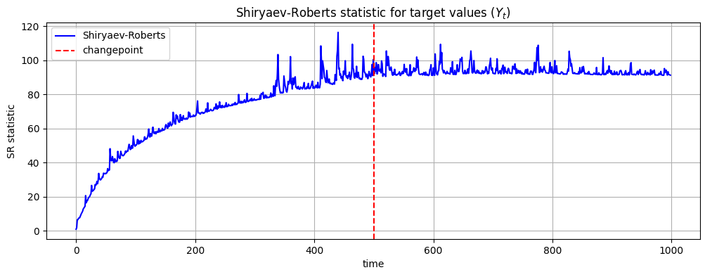
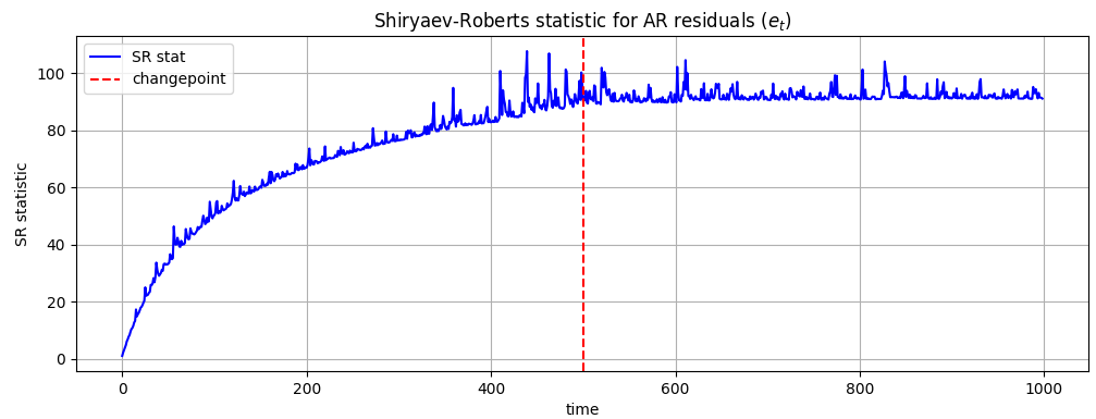
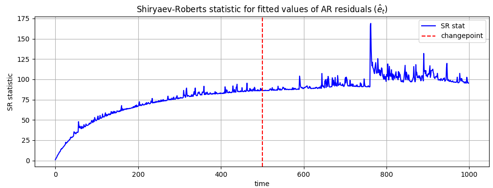
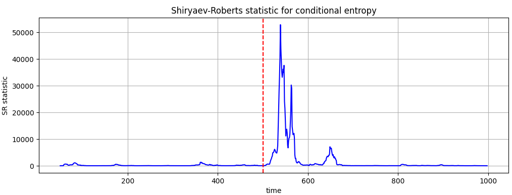
Figure 1 shows the values of respective SR statistics and the location of the change-point (vertical dashed line). It is clear from the figure that the traditional ways of applying the SR procedure fail to detect the change point. The SR statistics for three of the four figures grows with time and flattens out near the change-point but no spikes are large enough to trigger an alarm. On the other hand, the entropy-based procedure shown on the lower right panel produced an immediate and strong alarm.
This difference in performance is due to the limitation of traditional approaches. When applied to specific variables, as opposed to the entropy, they seem to target shifts of specific nature, e.g., shifts in mean, variance, autocorrelation. In this case, the shift in mean is too small. A key advantage of our approach is that it captures jumps in information transfer. In this sense, instead of analyzing various shifts in SR statistics, each verifying the presence of a specific drift, the entropy-based measure directly addresses stability of the dependence structure.
5.3 Non-linearity and ranks
We now turn to detection of termination and inversion of information transfer using the extensions of the entropy-based approach, that is, using local linear forests and ranks. The simulation designs are as described in Section 5.1. Simulation results are summarized in Figures (2)-(3), where denotes the moment of change, denotes the moment of change detection and is the threshold value used for the Shiryaev-Roberts statistic. The window length is .
It follows from Figures (2)-(3) that all extensions to the baseline entropy-based methods work very well in all four setups. There is not clear ordering in performance among the four setups: (a) baseline version (linear model, no ranks); (b) extension with LLF (local linear forest, no ranks); (c) extension with ranks of (linear model, ranks); (d) extension with ranks of (local linear forest, ranks). For both termination and inversion, all four are able to trigger an alarm within 7-15 time periods, using the respective thresholds. Table 2 summarizes this finding.
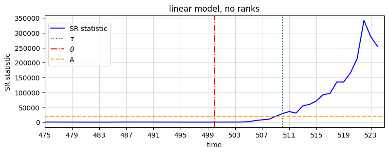


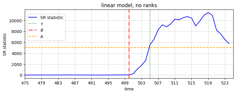
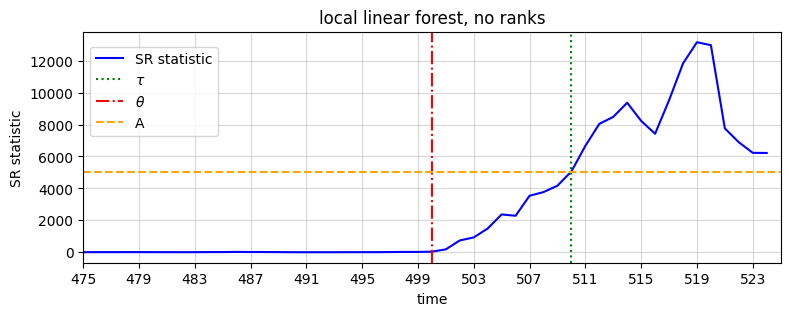
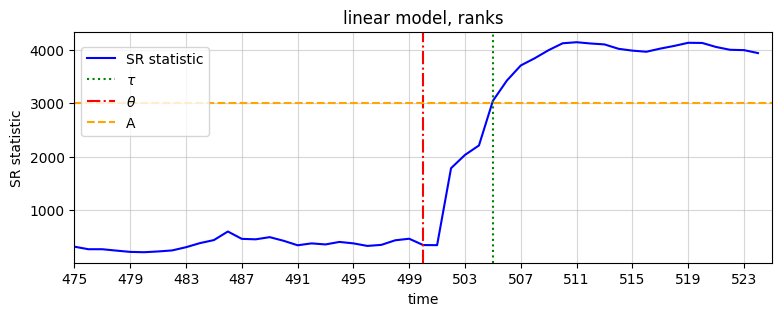
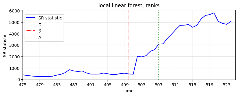
Interestingly, a comparison between the lower and upper panels of the figures suggests that PFA for ranks is higher than for levels, as can be seen by the non-zero values of SR before the break in the lower panels (and zero SR in the upper panels). However, this does not allow us to clearly identify cases when rank-based measures may or may not be preferred, which is addressed in the next subsection.
| Model | Termination | Inversion |
|---|---|---|
| linear | 10 | 5 |
| LLF | 9 | 10 |
| linear + ranks | 9 | 5 |
| LLF + ranks | 15 | 7 |
5.4 Heavy tails and tail-dependence
To further investigate the benefits of rank-based measures we consider a setting where the heavy tailed property of individual distributions prevents a productive use of such characteristics as the mean, variance or correlations. This setting is of particular relevance for financial data from emerging markets which are known to be extremely volatile.
We modify the simulation design of the previous sections by including a component with heavy-tailed data and tail dependence. For this purpose we add a penalty to a simplified version of termination of information flow as follows:
where . The role of is to control the noise level depending on how close the observation is to the sample median. Let denote such a distance. We define as follows:
Clearly, the closer an observation is to the median the more noise has over . For the observations closer to the sample extremes, is closer to being perfectly collinear with . This produces non-zero tail-dependence, that is non-zero correlation between and closer to the extremes of these variables. Additionally, we use the Weibull minimum extreme value distribution for to induce the heavy-tailed property.
Figure 4 plots the conditional entropy processes obtained using the four methods we consider: (a) the baseline linear model based on levels, (b) the local linear forest model based on levels, (c) the linear model based on ranks, (d) the local linear forest model based on ranks. The vertical dashed line indicates the change point ().
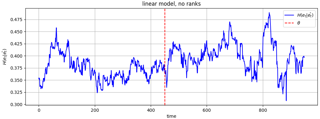
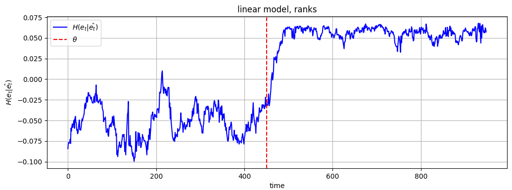
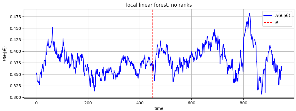
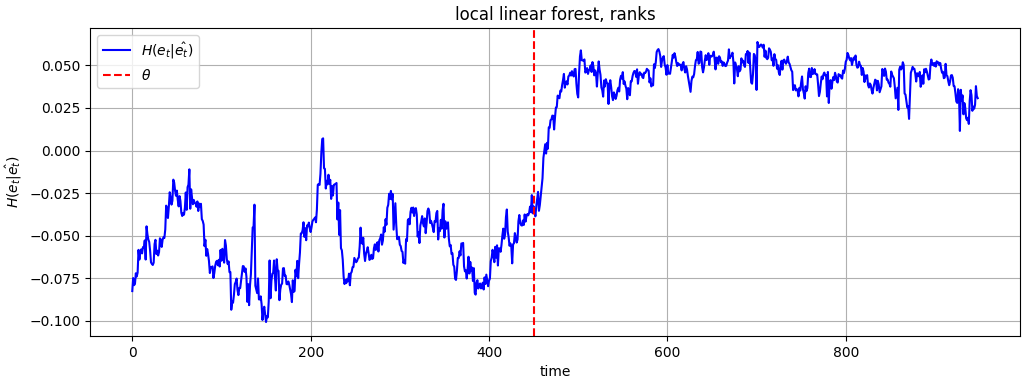
It is evident from Figure 4 even without computing the entropy-based SR statistic that this approach fails to detect the regime shift based on the original data (the upper and lower left panels do not show a visibly significant change in ), while the rank-based EWS provides consistent results and rapidly detects the regime shift (the upper and lower right panels show a clear jump to a new mean of after the change point). This suggests that the new rank-based methodology is attractive in cases when the financial data are leptokurtic and tail-dependent.
5.5 Comparison with other detection methods
Finally, we compare the proposed methods with non-SR approaches to concept drift detection from computer science such as Early Drift Detection Method (EDDM) and Adaptive Windowing Method (ADWIN) of Bifet and Gavalda (2007), and Kolmogorov-Smirnov Windowing Method (KSWIN) of Raab et al. (2020) and from economics such as an online version of the structural breaks detection method of Bai and Perron (1998). We focus on information transfer termination from Section 5.1.
Since EDDM, ADWIN and KSWIN are designed to operate on univariate time series they needed to be adapted to be comparable with our methods. Similarly, the Bai-Perron test, being an offline test, needed to be turned into an online procedure. A perfectly fair comparison is impossible here. The compromise we use is as follows:
(a) For ADWIN, EDDM, and KSWIN, we split time series into non-overlapping segments of length 50, i.e., For each segment we obtain residuals , where and are computed according to Eqs.(6) and (7), respectively. We then concatenate these segments and apply the relevant algorithms to it. We repeat this for 100 replications and compute PFA (probability of false alarm), ADD (average detection delay) and ND (fraction of non-detections).
(b) For the Bai-Perron test, we apply the test at the 1% significance level to an expanding window of data starting with and expanding it to We stop when the test reject the null. We repeat this over 100 replications and compute PFA, ADD and ND.
(c) For our methods, we apply them as described in Section 3 (baseline) and 4.1 (LLF), with window length 50, . We repeat this over 100 replications and compute compute PFA, ADD and ND.
| Metric | ADWIN | EDDM | KSWIN | Bai-Perron | baseline | LLF |
|---|---|---|---|---|---|---|
| PFA | - | - | 0.89 | 0.66 | 0.1 | 0.09 |
| ADD | - | - | 8.5 | 23.6 | 10.1 | 10.4 |
| ND | 1 | 1 | 0.09 | 0 | 0.05 | 0.04 |
The results are summarized in Table 3. Using this simulation design, both ADWIN and EDDM failed to detect the break, while KSWIN detected it in 91% of replications and produced a false alarm in of replications. This implies that there are only of replications where KSWIN detected the drift correctly. The Bai-Perron test detected all drifts, which is perhaps expected given the repeated testing problem implied by algorithm (b). It also produced 66% false positives. The proposed methods strongly dominate the alternatives in this exercise both in terms of PFA and ADD.
6 Empirical applications
We provide two empirical illustrations of how our approach can be used in constructing an early warning system in macroeconomic data.
6.1 Uzbekistan: spillover from commodity markets
First, we study the dynamics of the Uzbekistan equity market as measured by the Uzbekistan Composite Index (UCI). UCI is weighted average of stock prices traded on Tashkent Stock Exchange; Appendix A provides a list of data sources used in the section, including UCI. All prices are daily open and log-returns.
According to a 2022 World Bank report, commodity market plays a pivotal role for this economy, for example, gold and cotton make up and of the country’s export, respectively.333“Toward a Prosperous and Inclusive Future : The Second Systematic Country Diagnostic for Uzbekistan (English)”. Washington, D.C. : World Bank Group. http://documents.worldbank.org/curated/en/933471650320792872/Toward-a-Prosperous-and-Inclusive-Future-The-Second-Systematic-Country-Diagnostic-for-Uzbekistan Imports structure is more homogeneous. with refined petroleum ( of the country’s imports) and wheat ( of imports) making up the largest imports shares. It is natural to assume that the equity market of this open economy is susceptible to shocks from the global commodity markets. Therefore, we investigate information transfer from commodity prices to UCI, where the list of commodities includes gold, wheat, cotton and crude oil. We consider daily data from 1 January 2021 to 30 November 2022; Table 4 reports the summary statistics for the entire period.
| mean | std | skewness | kurtosis | rank | ||
|---|---|---|---|---|---|---|
| UCI | 0.000 | 0.047 | -0.226 | 14.259 | -0.075 | -0.049 |
| Crude oil | 0.000 | 0.027 | -0.523 | 3.636 | -0.013 | 0.028 |
| Gold | 0.000 | 0.009 | -0.238 | 1.844 | -0.023 | -0.009 |
| Wheat | 0.000 | 0.022 | 0.309 | 3.413 | -0.025 | -0.024 |
| Cotton | 0.000 | 0.023 | -2.202 | 23.497 | 0.018 | -0.012 |
We use a sliding window of 100 days to estimate the conditional entropy process as described in Section 4.1. The order of the AR process for UCI is picked by BIC and is different for each sliding window; the largest lag of explanatory variables in Eq. (7) is three but we conducted sensitivity analysis to this parameters varying between 1 and 10 with no significance difference to the results. The number of shifts , the exponential smoothing parameters are and as in the simulations.
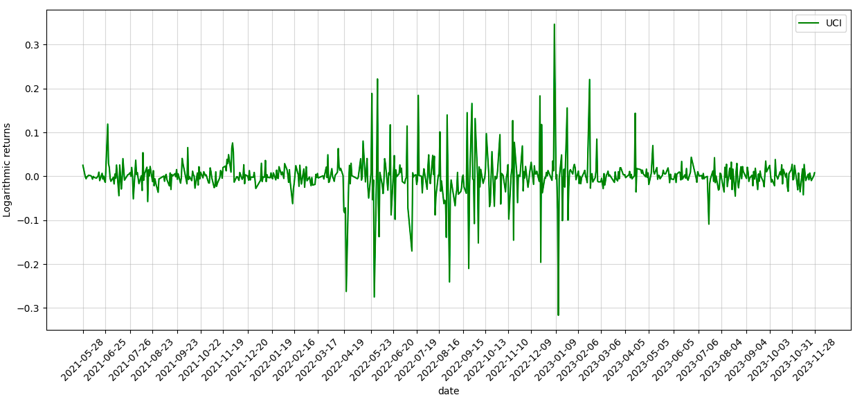
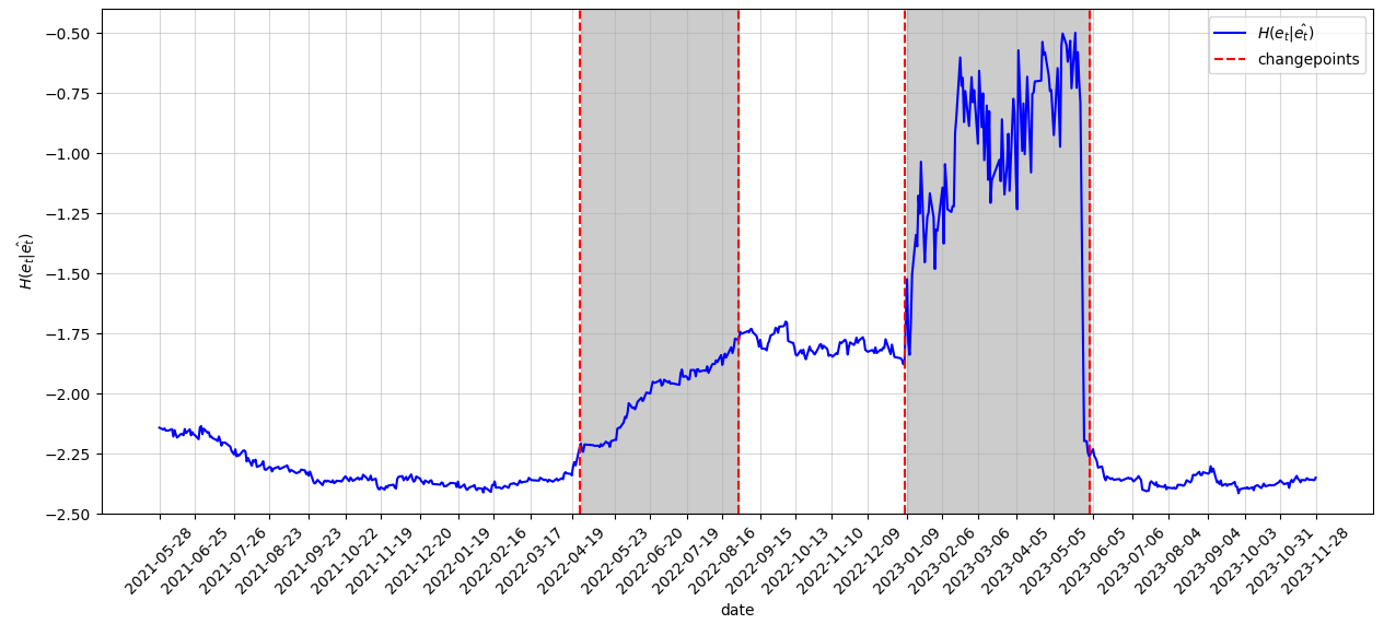
Figure 5 plots the resulting conditional entropy, together with the log-return of UCI. The figure reports five distinct regimes detected by this EWS. They are identified by vertical dashed lines and shaded areas on the figure. The dates and summary statistics for each regime are reported in Table 5.
| regime | mean | std | skewness | kurtosis | rank | |
|---|---|---|---|---|---|---|
| 2021.05.28 - 2022.04.25 | 0.002 | 0.022 | -3.051 | 30.794 | 0.229 | -0.021 |
| 2022.04.26 - 2022.08.29 | -0.008 | 0.077 | -0.346 | 3.586 | -0.165 | -0.107 |
| 2022.08.30 - 2023.01.07 | 0.001 | 0.073 | 1.010 | 5.782 | -0.273 | -0.194 |
| 2023.01.08 - 2023.06.02 | 0.002 | 0.050 | -1.404 | 19.710 | -0.036 | -0.0620 |
| 2023.06.03 - 2023.11.28 | -0.001 | 0.020 | -1.178 | 5.380 | -0.147 | -0.255 |
The detected regimes are not visible in the original UCI return series except perhaps for the first change point which coincides with a noticeable increase in UCI volatility. This is not surprising given that conditional entropy captures the aggregate partial effect of the commodity markets. The five regimes are as follows: (a) a low entropy period, (b) a slowly rising entropy period, (c) a stabilization period, (d) an entropy hike period, and (e) a return to normal period. Regime (d) is perhaps surprising and must reflect a disconnect between the equity and commodity markets in that period.
6.2 Russia: conflict in Ukraine and industrial spillover
Next we ask a similar question about the Russian equity market, using the Russian Trading System Index (RTS) as an indicator of the state of the Russian financial sector. RTS is a capitalization-weighted composite index computed using prices of the 50 most liquid Russian stocks traded on the Moscow Exchange.
According to the 2022 data from International Trade Center, which is a joint agency of the United Nations and the World Trade Organization444See https://www.trademap.org/Index.aspx, crude oil and natural gas made up and of Russia’s exports, respectively, which makes them the largest components of the country’s exports. It is therefore reasonable to expect that the global prices of these commodities contain important information for constructing an EWS for the Russian equity market. Similarly, machinery makes up the most important part in the structure of Russia’s imports ( of imports). Therefore, we use daily log-returns on open prices of crude oil, natural gas as well as S&P500 machinery index as the explanatory variables, when exploring the information transfer between these markets. Table 6 reports the summary statistics. The period we use is from 1 January 2021 to 30 November 2023 excluding the period between 24 February 2022 and 24 March 2022, when trading on RTS was suspended. We use the same parameters for the SR algorithm as in the previous subsection.
| mean | std | skewness | kurtosis | rank | ||
|---|---|---|---|---|---|---|
| RTS | 0.000 | 0.084 | 0.663 | 15.59 | -0.285 | -0.121 |
| SnP500 Machinery | 0.000 | 0.012 | -0.044 | 1.390 | -0.015 | 0.024 |
| Natural gas | 0.000 | 0.101 | -1.222 | 31.737 | 0.0461 | -0.037 |
| Crude oil | 0.000 | 0.027 | -0.523 | 3.636 | -0.013 | 0.028 |
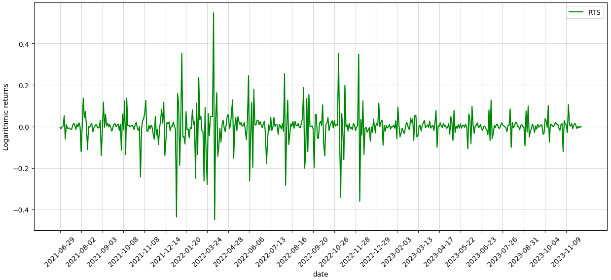
Figure 6 plots the log-returns of RTS and estimated conditional entropy. We can see from the figure that the EWS detects 3 distinct regimes where the structure of information flows changes significantly. The timing of the first shift likely corresponds to the increased economic uncertainty associated with the start of the Russian-Ukrainian military conflict on 24 February 2022. The shaded period is characterized by increased volatility, exacerbated by swift introduction of capital controls, gradual imposition of sanctions against the Russian economy and increased uncertainty regarding its long term prospects. Interestingly, the period ends by early September 2022 and the conditional entropy level returns to the pre-conflict level and goes even lower as economic outlook of the country proves to be better than anticipated.
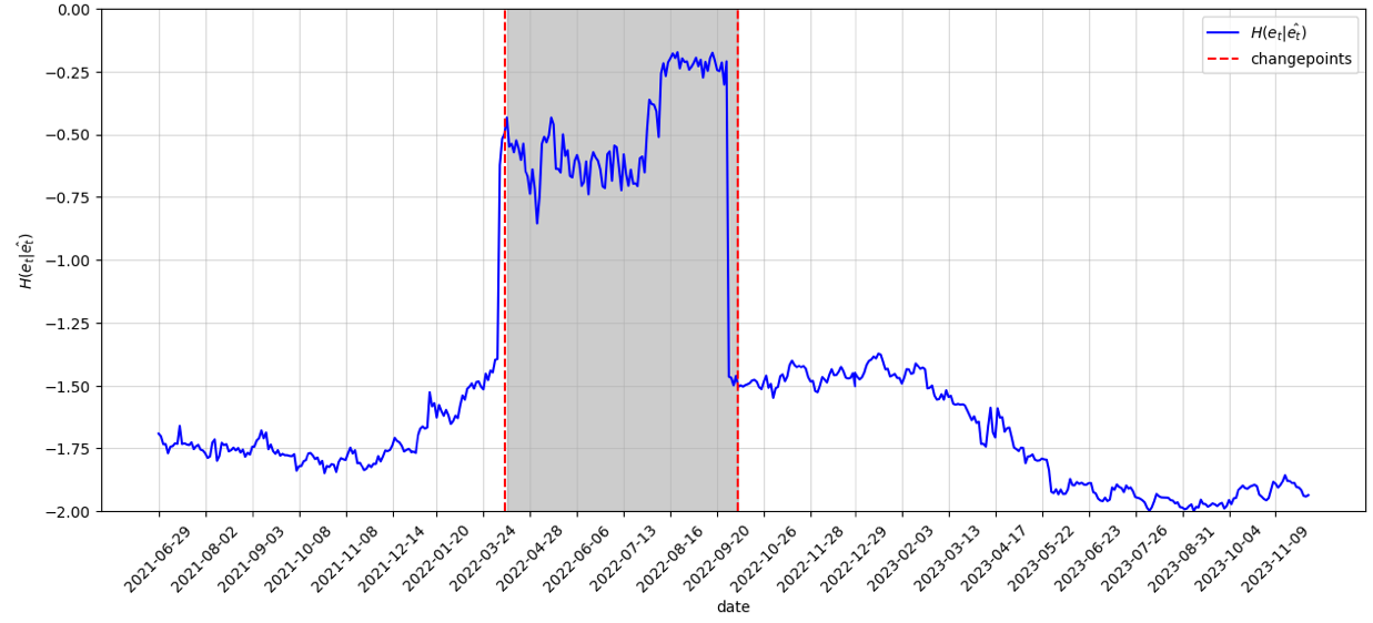
| regime | mean | std | skewness | kurtosis | rank | |
|---|---|---|---|---|---|---|
| 2021.06.29- 2022.03.10 | -0.003 | 0.084 | 1.280 | 14.107 | -0.249 | -0.070 |
| 2022.03.11 - 2022.10.11 | -0.001 | 0.130 | 0.146 | 6.868 | -0.373 | -0.192 |
| 2022.10.12 - 2023.11.30 | 0.001 | 0.061 | 0.041 | 16.768 | -0.351 | -0.233 |
7 Concluding remarks
We developed a new early warning system for concept drift detection via conditional entropy estimation. This is an original approach that combines benefit of information theory and machine learning to help monitor the level of uncertainty, remaining after accounting for lags of the target and explanatory variables. This approach is particularly relevant for modeling information flows in emerging markets which are characterized by repeated structural breaks and heavy tails in the data distribution.
We suggested a baseline methods based on a new conditional density estimator using random forest weights, and we worked out two extensions to the baseline that better capture non-linear interactions and accommodate heavy-tailed distributions. The extensions use a local linear forest estimator of the conditional mean and a rank-based estimator of the conditional copula density, respectively.
We illustrate the use of the new EWS on synthetic and real-life data. The simulation results show when the conventional SR statistic and alternative approached from machine learning and economics fail while the new approach provides robust performance. Fundamentally, the proposed methods are a first step towards leveraging recent advances in machine learning and statistic for automated market monitoring that may be used for many purposes but has particular relevance for markets with pronounced volatility, structural breaks, heavy tails and tail-dependence.
References
- Ahmad et al. (2018) Ahmad, W., A. V. Mishra, and K. J. Daly (2018): “Financial connectedness of BRICS and global sovereign bond markets,” Emerging Markets Review, 37, 1–16.
- Alanqary et al. (2021) Alanqary, A., A. Alomar, and D. Shah (2021): “Change Point Detection via Multivariate Singular Spectrum Analysis,” in Advances in Neural Information Processing Systems, ed. by M. Ranzato, A. Beygelzimer, Y. Dauphin, P. Liang, and J. W. Vaughan, Curran Associates, Inc., vol. 34, 23218–23230.
- Bai and Perron (1998) Bai, J. and P. Perron (1998): “Estimating and Testing Linear Models with Multiple Structural Changes,” Econometrica, 66, 47–78.
- Bai and Perron (2003) ——— (2003): “Computation and analysis of multiple structural change models,” Journal of Applied Econometrics, 18, 1–22.
- Baidari and Nagaraj (2021) Baidari, I. and H. Nagaraj (2021): “Bhattacharyya Distance Based Concept Drift Detection Method for Evolving Data Stream,” Expert Systems with Applications, 183.
- Barros (2018) Barros, R. S. M. d. e. a. (2018): “Wilcoxon Rank Sum Test Drift Detector,” Neurocomputing, 275, 1954–1963.
- Bhattacharyya (1943) Bhattacharyya, A. K. (1943): “On a Measure of Divergence between Two Statistical Populations Defined by Their Probability Distributions,” Bulletin of the Calcutta Mathematical Society, 35, 99–109.
- Bifet and Gavalda (2007) Bifet, A. and R. Gavalda (2007): “Learning from Time-Changing Data with Adaptive Windowing,” Proceedings of the Seventh SIAM International Conference on Data Mining.
- Breiman (2001) Breiman, L. (2001): “Random Forests,” Machine Learning, 45, 5–32.
- Caporale et al. (2020) Caporale, G. M., L. A. Gil-Alana, and C. Poza (2020): “Persistence, non-linearities and structural breaks in European stock market indices,” The Quarterly Review of Economics and Finance, 77, 50–61.
- Chaudhuri and Wu (2003) Chaudhuri, K. and Y. Wu (2003): “Random walk versus breaking trend in stock prices: Evidence from emerging markets,” Journal of Banking & Finance, 27, 575–592.
- Chen (2019) Chen, H. (2019): “Sequential change-point detection based on nearest neighbors,” Annals of Statistics, 47, 1381 – 1407.
- Chen et al. (2022) Chen, Z., M. Han, H. Wu, M. Li, and X. Zhang (2022): “A multi-level weighted concept drift detection method,” Journal of Supercomputing, 79, 5154–5180.
- Chen and Ibragimov (2019) Chen, Z. and R. Ibragimov (2019): “One country, two systems? The heavy-tailedness of Chinese A- and H- share markets,” Emerging Markets Review, 38, 115–141.
- Cherubini et al. (2011) Cherubini, U., S. Mulinacci, F. Gobbi, and S. Romagnoli (2011): Dynamic Copula Methods in Finance, Wiley Finance Series, John Wiley and Sons Ltd.
- Chu and Chen (2019) Chu, L. and H. Chen (2019): “Asymptotic distribution-free change-point detection for multivariate and non-euclidean data,” Annals of Statistics, 47, 382 – 414.
- Ditzler and Polikar (2011) Ditzler, G. and R. Polikar (2011): “Hellinger Distance Based Drift Detection for Nonstationary Environments,” IEEE Symposium on Computational Intelligence in Dynamic and Uncertain Environments (CIDUE).
- Friedberg et al. (2021) Friedberg, R., J. Tibshirani, S. Athey, and S. Wager (2021): “Local Linear Forests,” Journal of Computational and Graphical Statistics, 30, 503–517.
- Granger (1969) Granger, C. W. (1969): “Investigating causal relations by econometric models and cross-spectral methods,” Econometrica, 424–438.
- Guo et al. (2022) Guo, Y., M. Gao, and X. Lu (2022): “Multivariate change point detection for heterogeneous series,” Neurocomputing, 510, 122–134.
- Hamilton (2016) Hamilton, J. (2016): “Macroeconomic Regimes and Regime Shifts,” Elsevier, vol. 2 of Handbook of Macroeconomics, 163–201.
- Hartley (1928) Hartley, R. (1928): “Transmission of information,” Bell System Technical Journal, 535–563.
- Hoens (2012) Hoens, R. e. a. (2012): “Learning from Streaming Data with Concept Drift and Imbalance: An Overview,” Progress in Artificial Intelligence, 1, 89–101.
- Ibragimov and Prokhorov (2017) Ibragimov, R. and A. Prokhorov (2017): Heavy tails and copulas: Topics in dependence modelling in economics and finance, World Scientific Publishing: Singapore.
- Khalfaoui et al. (2023) Khalfaoui, R., S. Hammoudeh, and M. Z. Rehman (2023): “Spillovers and connectedness among BRICS stock markets, cryptocurrencies, and uncertainty: Evidence from the quantile vector autoregression network,” Emerging Markets Review, 54, 101002.
- Li and Racine (2023) Li, Q. and J. S. Racine (2023): Nonparametric econometrics: theory and practice, Princeton University Press.
- Neaime (2016) Neaime, S. (2016): “Financial crises and contagion vulnerability of MENA stock markets,” Emerging Markets Review, 27, 14–35.
- Orlitsky (2003) Orlitsky, A. (2003): “Information Theory,” in Encyclopedia of Physical Science and Technology (Third Edition), ed. by R. A. Meyers, New York: Academic Press, 751–769, third edition ed.
- Pepelyshev and Polunchenko (2017) Pepelyshev, A. and A. S. Polunchenko (2017): “Real-time financial surveillance via quickest change-point detection methods,” Statistics and its Interface, 93–106.
- Pergamenchtchikov and Tartakovsky (2018) Pergamenchtchikov, S. and A. G. Tartakovsky (2018): “Asymptotically optimal pointwise and minimax quickest change-point detection for dependent data,” Statistical Inference for Stochastic Processes, 21, 217 – 259.
- Pergamenchtchikov and Tartakovsky (2019) ——— (2019): “Asymptotically optimal pointwise and minimax change-point detection for general stochastic models with a composite post-change hypothesis,” Journal of Multivariate Analysis, 174.
- Polunchenko and Tartakovsky (2010) Polunchenko, A. S. and A. G. Tartakovsky (2010): “On Optimality of the Shiryaev-Roberts Procedure for Detecting a Change in Distribution,” The Annals of Statistics, 38, 3445–3457.
- Pospisil and Lee (2018) Pospisil, T. and A. B. Lee (2018): “RFCDE: Random Forests for Conditional Density Estimation,” arXiv preprint arXiv:1804.05753.
- Probst et al. (2019) Probst, P., M. N. Wright, and A.-L. Boulesteix (2019): “Hyperparameters and tuning strategies for random forest,” WIREs Data Mining and Knowledge Discovery, 9, e1301.
- Raab et al. (2020) Raab, C., M. Heusinger, and F.-M. Schleif (2020): “Reactive soft prototype computing for concept drift streams,” Neurocomputing, 340–351.
- Roberts (1966) Roberts, S. (1966): “A Comparison of Some Control Chart Procedures,” Technometrics, 411–430.
- Shannon (1948) Shannon, C. (1948): “A mathematical theory of communication,” Bell System TechnicalJournal, 27, 379–423.
- Shiryaev (1963) Shiryaev, A. (1963): “On Optimum Methods in Quickest Detection Problems,” Probability Theory Application, 8, 22–46.
- Shiryaev (1961) Shiryaev, A. N. (1961): “The problem of the most rapid detection of a disturbance in a stationary process,” in Soviet Math. Dokl, vol. 2, 103.
- Smimou and Khallouli (2015) Smimou, K. and W. Khallouli (2015): “Does the Euro affect the dynamic relation between stock market liquidity and the business cycle?” Emerging Markets Review, 25, 125–153.
- Tajeuna et al. (2023) Tajeuna, E. G., M. Bouguessa, and S. Wang (2023): “Modeling Regime Shifts in Multiple Time Series,” ACM Transactions on Knowledge Discovery from Data, 17.
- Tartakovsky and Spivak (2021) Tartakovsky, A. and V. Spivak (2021): “Analysis of the Weighted Shiryaev–Roberts Procedure in the Problem of Changepoint Detection for Models with Unknown Post Change Parameters.” Works of MIPT, Computer Science and Management, 13.
- Tartakovsky (2016) Tartakovsky, A. G. (2016): “On Asymptotic Optimality in Sequential Changepoint Detection: Non-iid Case,” ArXiv:1510.03827.
- Wang (2023) Wang, Shusen, e. a. (2023): “Unsupervised Concept Drift Detection for Time Series on Riemannian Manifolds,” Journal of the Franklin Institute, 13186–13204.
- Yang et al. (2023) Yang, Y., L. Zhao, Y. Zhu, L. Chen, G. Wang, and C. Wang (2023): “Spillovers from the Russia-Ukraine conflict,” Research in International Business and Finance, 66, 102006.
- Zhao et al. (2022) Zhao, H., J. Li, Y. Lei, and M. Zhou (2022): “Risk spillover of banking across regions: Evidence from the belt and road countries,” Emerging Markets Review, 52, 100919.
Appendix A Data sources
The following sources were used to obtain the data for Section 6:
-
Uzbekistan:
-
–
Uzbekistan Composite Index: https://uzse.uz/price_indices/
-
–
Brent Crude Oil Continuous Contract: https://www.marketwatch.com/investing/future/brn00
- –
- –
-
–
Cotton spot: https://finance.yahoo.com/quote
-
–
-
Russia:
-
–
Russian Trading System (RTS) Index: https://www.moex.com/en/index/RTSI/archive
-
–
S&P industrials: https://www.spglobal.com/spdji
-
–
Oil prices: https://www.marketwatch.com
-
–
Natural gas prices: https://www.eia.gov
-
–