Spatio-Spectral Structure Tensor Total Variation for Hyperspectral Image Denoising and Destriping

Abstract

This paper proposes a novel regularization method, named Spatio-Spectral Structure Tensor Total Variation (${\text{S}_{3}\text{TTV}}$), for denoising and destriping of hyperspectral (HS) images. HS images are inevitably contaminated by various types of noise, during acquisition process, due to the measurement equipment and the environment. For HS image denoising and destriping tasks, Spatio-Spectral Total Variation (SSTV), defined using second-order spatio-spectral differences, is widely known as a powerful regularization approach that models the underlying spatio-spectral properties. However, since SSTV refers only to adjacent pixels/bands, semi-local spatial structures are not preserved during denoising process. To address this problem, we newly design ${\text{S}_{3}\text{TTV}}$, defined by the sum of the nuclear norms of matrices consisting of second-order spatio-spectral differences in small spectral blocks (we call these matrices as spatio-spectral structure tensors). The proposed regularization method simultaneously models the spatial piecewise-smoothness, the spatial similarity between adjacent bands, and the spectral correlation across all bands in small spectral blocks, leading to effective noise removal while preserving the semi-local spatial structures. Furthermore, we formulate the HS image denoising and destriping problem as a convex optimization problem involving ${\text{S}_{3}\text{TTV}}$ and develop an algorithm based on a preconditioned primal-dual splitting method to solve this problem efficiently. Finally, we demonstrate the effectiveness of ${\text{S}_{3}\text{TTV}}$ by comparing it with existing methods, including state-of-the-art ones through denoising and destriping experiments.

I Introduction

Hyperspectral (HS) imaging measures a wide spectrum of light ranging from the ultraviolet to the near-infrared. The rich spectral information of HS images, with more than one hundred bands, can distinguish materials and phenomena that the human eye and existing RGB cameras cannot. This capability has been applied in diverse fields including agriculture, mineralogy, astronomy, and biotechnology [1, 2, 3, 4]. However, observed HS images are inevitably contaminated by various types of noise—including thermal noise, quantization noise, shot noise, and stripe noise—due to factors caused by measurement equipment and environment, such as photon effects, atmospheric absorption, dark currents, and sensor disturbances [5, 6, 7]. Since such noise significantly degrades the performance of subsequent processing such as unmixing [8, 9], classification [10, 11, 12], and anomaly detection [13, 14], HS image denoising is an essential preprocessing step for the applications.

To recover desirable HS images from degraded observations, many existing methods design some regularization functions that mathematically model the inherent spatio-spectral structure in HS images and then solve optimization problems that incorporate the regularization functions. As a representative class of regularization methods for HS images, total variation (TV) type regularization methods have been developed. This approach originated from edge-preserving natural image denoising [15, 16], and the pioneering TV-type method for HS image denoising is Spectral-Spatial Adaptive Hyperspectral TV (SSAHTV) [17]. SSAHTV models the spatial piecewise-smoothness of HS images as the sparsity of first-order spatial differences between adjacent pixels. Furthermore, Anisotropic Spectral Spatial TV (ASSTV) [18] extends this model by incorporating first-order spectral differences into the SSAHTV regularization function, capturing the spectral piecewise-smoothness in addition to the spatial piecewise-smoothness of HS images. However, SSAHTV and ASSTV cause 1) over-smoothing by minimizing $\ell_{1}$-type norms of first-order differences, and 2) corruption of the semi-local spatial structures during the denoising process because they only refer to adjacent pixels/bands.

To mitigate these weaknesses, some regularization methods have combined ASSTV with an additional regularization function, specifically a low-rank (LR)-type regularization function [19, 20, 21]. The LR-type regularization functions are designed to capture the spectral correlation across all bands due to the fact that HS images are composed of a few variety of material-specific spectra. However, these methods have two other challenges: the mischaracterization of stripe noise (see Figs. 3, 4, and 6 in Sec. IV) and the difficulty of setting the parameter that balances the two different regularization functions. Therefore, our paper focuses on enhancing single TV-type regularization methods.

One promising single TV-type regularization method that overcomes over-smoothing is Spatio-Spectral TV (SSTV) [22]. SSTV is defined by the $\ell_{1}$ norm of second-order spatio-spectral differences, i.e., first-order spatial differences of spectral ones to avoid over-smoothing. In addition, SSTV captures not only the spatial piecewise-smoothness, but also the spatial similarity between adjacent bands by its formulation. For these reason, SSTV has been widely used in state-of-the-art HS image denoising methods [23, 24, 25, 26, 27]. Takeyama et al. proposed Hybrid Spatio-Spectral TV (HSSTV) [25], which enhances SSTV by incorporating SSAHTV. To recover more detailed spatial structures of HS images, Graph Spatio-Spectral TV (GSSTV) [27] was proposed, which weights the spatial difference operator of SSTV based on a graph reflecting the spatial structures of an HS image. To directly control the degree of the smoothness, Wang et al. proposed the $\ell_{0}\text{-}\ell_{1}$ hybrid TV (${l_{0}\text{-}l_{1}\text{HTV}}$) [26], which incorporates $\ell_{0}$-type constraints of the spatial differences (originally proposed for color image processing [28]) into SSTV. However, SSTV and its extension methods cannot preserve the semi-local spatial structures of HS images during the denoising process because they only refer to adjacent pixels/bands.

Other single TV-type regularization methods that preserve the semi-local spatial structures are the Structure tensor TV (STV)-type regularization methods [29, 30, 31, 32]. These regularization functions are defined as the sum of nuclear norms of structure tensors consisting of matrices of local differences in small spectral blocks containing small spatial areas and all bands. The original STV [29] and Structure Tensor total variation-regularized Weighted Nuclear Norm Minimization (STWNNM) [30] capture the semi-local spatial piecewise-smoothness, but do not model the spectral property of HS images due to consisting only of spatial differences. The regularization function of Arranged Structure tensor TV (ASTV) [31] characterizes the spectral correlations across all bands by modifying the ordering of spatial differences in the structure tensors. In addition, Spatio-Spectral Structure Tensor (SSST) [32] explicitly exploits the spectral piecewise-smoothness of HS images by including not only spatial differences but also spectral ones in its formulation. However, the existing STV-type regularization methods minimize the nuclear norms of “first-order” differences, leading to spatial or spectral over-smoothing, as in SSAHTV.

From the discussion so far, SSTV and STV-type regularization methods are powerful approaches that capture the underlying spatial and spectral characteristics of HS images. However, they have their own limitations: SSTV cannot preserve the semi-local spatial structures and STV-type regularization methods cause over-smoothing. Now a natural question arises: Can we design a regularization function with the four requirements: avoid over-smoothing, preserve semi-local spatial structures, effectively remove stripe noise, and be a single regularization function?

Inspired by both SSTV and the above family of STV, we propose a denoising method for HS images using a newly introduced spatio-spectral structure tensor total variation (${\text{S}_{3}\text{TTV}}$) model. The main contributions of this article are summarized as follows.

1. We design a novel formulation of an STV-type regularization method, namely ${\text{S}_{3}\text{TTV}}$. ${\text{S}_{3}\text{TTV}}$ is defined as the sum of the nuclear norms of newly designed structure tensors (called spatio-spectral structure tensor), each of which consists of second-order spatio-spectral differences within a small spectral block. ${\text{S}_{3}\text{TTV}}$ can be seen as a hybrid regularization function that is constructed by integrating SSTV and STV into a convex function, and thus can fully capture the spatial piecewise-smoothness, the spatial similarity between adjacent bands, and the spectral correlation across all bands of HS images. This leads to effective noise removal while preserving the semi-local spatial structures of HS images without over-smoothing.

2. We formulate the mixed noise removal problem as a constrained convex optimization problem involving ${\text{S}_{3}\text{TTV}}$. By including the functions that characterize Gaussian, sparse, and stripe noise in the optimization problem, the proposed method effectively removes the three types of noise. In this formulation, we model data-fidelity and noise terms as hard constraints instead of adding them to the objective function. This type of constrained formulation decouples interdependent hyperparameters into independent ones, making parameter setting easier. Such advantages are also addressed, for example, in [33, 34, 35, 36, 37, 38]. Furthermore, since the objective function has only a single regularization function, the proposed method does not require a balance parameter.

3. To solve our optimization problem for the HS image denoising, we develop an efficient algorithm based on a Preconditioned Primal-Dual Splitting method (P-PDS) [39]. Unlike other popular algorithms used in existing HS image denoising methods, such as an alternating direction method of multipliers [40] and PDS [41, 42], P-PDS can automatically determine the appropriate stepsizes based on the problem structure [39, 43].

Experimental results show the superiority of the proposed method to existing methods including state-of-the-art ones. The comparison of the features of the existing and proposed methods is summarized in Fig. I.

The paper is organized as follows. In Sec. II, we introduce the mathematical tools required for the proposed method. Sec. III provides the proposed HS image denoising method involving ${\text{S}_{3}\text{TTV}}$. The experimental results are reported in Sec. IV. Finally, we give concluding remarks in Sec. V. The preliminary version of this paper, without considering stripe noise, mathematical details, comprehensive experimental comparison, or deeper discussion, has appeared in conference proceedings [44].

TABLE I: Pros and Cons of Existing and Proposed Methods for HS Image Denoising.

Methods	Spatial piecewise smoothness	Spatial similarity between adjacent bands	Spectral correlation across all bands	Avoiding over-smoothing	Convexity
SSAHTV [17]	$\checkmark$	–	–	–	$\checkmark$
LRTDTV [20]	$\checkmark$	–	$\checkmark$	$\checkmark$	–
TPTV [21]	$\checkmark$	–	$\checkmark$	$\checkmark$	–
SSTV [22]	$\checkmark$	$\checkmark$	–	$\checkmark$	$\checkmark$
HSSTV [25]	$\checkmark$	$\checkmark$	–	–	$\checkmark$
GSSTV [27]	$\checkmark$	$\checkmark$	–	$\checkmark$	$\checkmark$
${l_{0}\text{-}l_{1}\text{HTV}}$ [26]	$\checkmark$	$\checkmark$	–	$\checkmark$	–
STV [29]	$\checkmark$	–	–	–	$\checkmark$
STWNNM [30]	$\checkmark$	–	–	–	–
ASTV [31]	$\checkmark$	–	$\checkmark$	–	$\checkmark$
SSST [32]	$\checkmark$	–	$\checkmark$	–	$\checkmark$
Proposed method	$\checkmark$	$\checkmark$	$\checkmark$	$\checkmark$	$\checkmark$

II Preliminaries

II-A Notations

Throughout this paper, we denote vectors and matrices by boldface lowercase letters (e.g., $\mathbf{x}$) and boldface capital letters (e.g., $\mathbf{X}$), respectively. We treat an HS image, denoted by $\mathbf{u}$ with $N_{1}$ vertical pixels, $N_{2}$ horizontal pixels, and $N_{3}$ bands. We denotes the total number of elements in the HS image by $N=N_{1}N_{2}N_{3}$. For a matrix data $\mathbf{X}\in\mathbb{R}^{N_{1}\times N_{2}}$, the value at the location $(i,j)$ is denoted by $[\mathbf{X}]_{i,j}$. The $\ell_{1}$-norm and the $\ell_{2}$-norm of a vector $\mathbf{x}\in\mathbb{R}^{N}$ are defined as $\|\mathbf{x}\|_{1}:=\sum_{n=1}^{N}|x_{n}|$ and $\|\mathbf{x}\|_{2}:=\sqrt{\sum_{n=1}^{N}x_{n}^{2}}$, respectively, where $x_{n}$ represents the $n$-th entry of $\mathbf{x}$. The nuclear norm of a marix, which is the sum of all the singular values, is denoted by $\|\cdot\|_{*}$. For an HS image $\mathbf{u}\in\mathbb{R}^{N}$, let $\mathbf{D}_{v}\in\mathbb{R}^{N\times N}$, $\mathbf{D}_{h}\in\mathbb{R}^{N\times N}$, and $\mathbf{D}_{s}\in\mathbb{R}^{N\times N}$ be the forward difference operators along the horizontal, vertical, and spectral directions, respectively, with the periodic boundary condition. Here, a spatial difference operator is denoted by $\mathbf{D}:=\begin{pmatrix}\mathbf{D}_{v}^{\top}&\mathbf{D}_{h}^{\top}\end{pmatrix}^{\top}\in\mathbb{R}^{2N\times N}$. Using $\mathbf{D}_{v}$, $\mathbf{D}_{h}$, and $\mathbf{D}_{s}$, we denote the second-order spatio-spectral differences by $\mathbf{D}_{v}\mathbf{D}_{s}\mathbf{u}\in\mathbb{R}^{N}$ and $\mathbf{D}_{h}\mathbf{D}_{s}\mathbf{u}\in\mathbb{R}^{N}$. Other notations will be introduced as needed.

II-B Proximal Tools

In this chapter, we introduce basic proximal tools that play a central role in the optimization part of our method.

For any $\gamma>0$, the proximity operator of $f$ is defined by

$$\operatorname{prox}_{\gamma,f}(\mathbf{x}):=\arg\min_{\mathbf{y}\in\mathbb{R}^{N}}f(\mathbf{y})+\frac{1}{2\gamma}\|\mathbf{x}-\mathbf{y}\|_{2}^{2}.$$ (1)

The Fenchel–Rockafellar conjugate function $f^{*}$ of the function $f$ is defined by

$$f^{*}(\mathbf{x}):=\sup_{\mathbf{y}}\langle\mathbf{x},\mathbf{y}\rangle-f(\mathbf{y}),$$ (2)

where $\langle\cdot,\cdot\rangle$ is the Euclidean inner product. Thanks to a generalization of Moreau’s identity [45], the proximity operator of $f^{*}$ is calculated as

$$\operatorname{prox}_{\gamma,f^{*}}(\mathbf{x})=\mathbf{x}-\gamma\operatorname{prox}_{\frac{1}{\gamma}f}\left(\frac{1}{\gamma}\mathbf{x}\right).$$ (3)

The indicator function of a nonempty closed convex set $C\subset\mathbb{R}^{N}$, denoted by $\iota_{C}$, is defined as

$$\iota_{C}(\mathbf{x}):=\begin{cases}0,&\mathrm{if}\>\mathbf{x}\in C,\\ \infty,&\mathrm{otherwise}.\end{cases}$$ (4)

The proximity operator of $\iota_{C}$ is equivalent to the projection onto $C$, as given by

$$\operatorname{prox}_{\iota_{C}}(\mathbf{x})=P_{C}(\mathbf{x}):=\mathop{\mathrm{argmin}}\limits_{\mathbf{y}\in C}\|\mathbf{y}-\mathbf{x}\|_{2}.$$ (5)

II-C Preconditoned Primal-Dual Splitting Method (P-PDS)

Consider the following generic form of convex optimization problems:

$$\min_{\begin{subarray}{c}\mathbf{x}_{1},\ldots,\mathbf{x}_{N},\\ \mathbf{y}_{1},\ldots,\mathbf{y}_{M}\end{subarray}} \sum_{i=1}^{N}f_{i}(\mathbf{x}_{i})+\sum_{j=1}^{M}g_{j}(\mathbf{y}_{j})$$

$$\mathrm{s.t.}\>\begin{cases}\mathbf{y}_{1}=\sum_{i=1}^{N}\mathbf{A}_{1,i}\mathbf{x}_{i},\\ \vdots\\ \mathbf{y}_{M}=\sum_{i=1}^{N}\mathbf{A}_{M,i}\mathbf{x}_{i},\end{cases}$$ (6)

where $f_{i}(i=1,\ldots,N)$ and $g_{j}(j=1,\ldots,M)$ are lower semi-continuous proper convex functions, $\mathbf{x}_{i}\in\mathbb{R}^{n_{i}}\>(i=1,\dots,N)$ are primal variables, $\mathbf{y}_{j}\in\mathbb{R}^{m_{j}}\>(j=1,\dots,M)$ are dual variables, and $\mathbf{A}_{j,i}\in\mathbb{R}^{m_{j}\times n_{i}}$ ($i=1,\ldots,N$, $j=1,\ldots,M$) are linear operators.

The standard PDS [41, 42] and P-PDS [39], on which our algorithm is based, solve Prob. (II-C) by the following iterative procedures:

$$\left\lfloor\begin{array}[]{l}\mathbf{x}_{1}^{(t+1)}\leftarrow\operatorname{prox}_{\gamma_{1,1},f_{1}}\left(\mathbf{x}_{1}^{(t)}-\gamma_{1,1}\bigl{(}\sum_{j=1}^{M}\mathbf{A}_{j,1}^{\top}\mathbf{y}_{j}^{(t)}\bigr{)}\right),\\ \vdots\\ \mathbf{x}_{N}^{(t+1)}\leftarrow\operatorname{prox}_{\gamma_{1,N},f_{N}}\left(\mathbf{x}_{N}^{(t)}-\gamma_{1,N}\bigl{(}\sum_{j=1}^{M}\mathbf{A}_{j,N}^{\top}\mathbf{y}_{j}^{(t)}\bigr{)}\right),\\ \mathbf{x}_{i}^{{}^{\prime}}=2\mathbf{x}_{i}^{(t+1)}-\mathbf{x}_{i}^{(t)}\>(\forall i=1,\ldots,N),\\ \mathbf{y}_{1}^{(t+1)}\leftarrow\operatorname{prox}_{\gamma_{2,1},g_{1}^{*}}\left(\mathbf{y}_{1}^{(t)}-\gamma_{2,1}\bigl{(}\sum_{i=1}^{N}\mathbf{A}_{1,i}\mathbf{x}_{i}^{{}^{\prime}}\bigr{)}\right),\\ \vdots\\ \mathbf{y}_{M}^{(t+1)}\leftarrow\operatorname{prox}_{\gamma_{2,M},g_{M}^{*}}\left(\mathbf{y}_{M}^{(t)}-\gamma_{2,M}\bigl{(}\sum_{i=1}^{N}\mathbf{A}_{M,i}\mathbf{x}_{i}^{{}^{\prime}}\bigr{)}\right),\\ \end{array}\right.$$ (7)

where $\gamma_{1,i}(i=1,\dots,N)$ and $\gamma_{2,j}(j=1,\dots,M)$ are the stepsize parameters. The standard PDS needs to adjust the appropriate stepsize parameters to satisfy the convergence conditions. On the other hand, P-PDS can automatically determine the stepsize parameters that guarantee convergence [39, 43]. According to [39], this paper designs the stepsize parameters as follows:

$$\gamma_{1,i} =\frac{1}{\sum_{j=1}^{M}\sum_{l=1}^{m_{j}}|[\mathbf{A}_{j,i}]_{l,1}|},\>(\forall i=1,\ldots,N),$$

$$\gamma_{2,j} =\frac{1}{\sum_{i=1}^{N}\sum_{k=1}^{n_{i}}|[\mathbf{A}_{j,i}]_{1,k}|},\>(\forall j=1,\ldots,M).$$ (8)

III Proposed Method

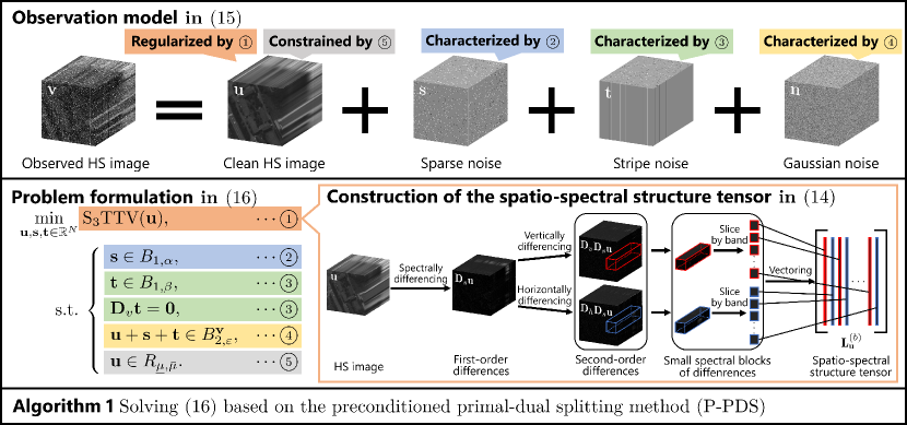
Figure 1: Illustration of the proposed method, i.e., ${\text{S}_{3}\text{TTV}}$.

In the following, we first describe the design of the ${\text{S}_{3}\text{TTV}}$ regularization function. Next, we consider a situation where an HS image is contaminated with mixed noise and introduce the corresponding observation model. Based on this model, we formulate an HS image denoising problem as a constrained convex optimization problem involving the ${\text{S}_{3}\text{TTV}}$ regularization function. Finally, we derive an algorithm based on P-PDS to efficiently solve the optimization problem. A schematic diagram of ${\text{S}_{3}\text{TTV}}$ is shown in Fig. 1.

III-A Spatio-Spectral Structure Tensor Total Variation (${\text{S}_{3}\text{TTV}}$)

Before describing the proposed regularization function, we introduce the notion of spatio-spectral structure tensor. First, for a given HS image $\mathbf{u}$, we calculate the second-order spatial-spectral differences $\mathbf{D}_{v}\mathbf{D}_{s}\mathbf{u}$ and $\mathbf{D}_{h}\mathbf{D}_{s}\mathbf{u}$. Next, we extract small spectral blocks by cropping the second-order spatio-spectral differences to the size $N_{1}^{{}^{\prime}}\times N_{2}^{{}^{\prime}}(N_{1}^{{}^{\prime}}<<N_{1},N_{2}^{{}^{\prime}}<<N_{2})$ for all bands. Then, the $b$-th spatio-spectral structure tensor $\mathbf{L}_{\mathbf{u}}^{(b)}$ is defined by vectorizing the second-order spatio-spectral differences in the $b$-th small spectral block by band and arranging them in parallel as follows:

$$\begin{split}\mathbf{L}_{\mathbf{u}}^{(b)}:=&\bigl{(}[\mathbf{D}_{v}\mathbf{D}_{s}\mathbf{u}]_{1}^{(b)}\>[\mathbf{D}_{h}\mathbf{D}_{s}\mathbf{u}]_{1}^{(b)}\\ &\quad\cdots[\mathbf{D}_{v}\mathbf{D}_{s}\mathbf{u}]_{N_{3}}^{(b)}\>[\mathbf{D}_{h}\mathbf{D}_{s}\mathbf{u}]_{N_{3}}^{(b)}\bigr{)}\in\mathbb{R}^{N_{1}^{{}^{\prime}}N_{2}^{{}^{\prime}}\times 2N_{3}}.\end{split}$$ (9)

where $[\mathbf{D}_{v}\mathbf{D}_{s}\mathbf{u}]_{i}^{(b)}\in\mathbb{R}^{N_{1}^{{}^{\prime}}N_{2}^{{}^{\prime}}}$ and $[\mathbf{D}_{h}\mathbf{D}_{s}\mathbf{u}]_{i}^{(b)}\in\mathbb{R}^{N_{1}^{{}^{\prime}}N_{2}^{{}^{\prime}}}$ are the second-order spatio-spectral differences of $i$-th band in the $b$-th small spectral block. Since HS images have the strong correlation across all bands, $[\mathbf{D}_{v}\mathbf{D}_{s}\mathbf{u}]_{1}^{(b)},\ldots,[\mathbf{D}_{v}\mathbf{D}_{s}\mathbf{u}]_{N_{3}}^{(b)}$ and $[\mathbf{D}_{h}\mathbf{D}_{s}\mathbf{u}]_{1}^{(b)},\ldots,[\mathbf{D}_{h}\mathbf{D}_{s}\mathbf{u}]_{N_{3}}^{(b)}$ are similar vectors, respectively, i.e., the columns of $\mathbf{L}_{\mathbf{u}}^{(b)}$ are approximately linearly dependent. The flow of constructing the spatio-spectral structure tensor is depicted in the middle right of Fig. 1.

To capture the spatial piecewise-smoothness, the spatial similarity between adjacent bands, and the spectral correlation of an HS image, we propose a regularization function using the spatio-spectral structure tensors as follows:

$$\textstyle{\text{S}_{3}\text{TTV}}(\mathbf{u}):=\sum_{b=1}^{B}\|\mathbf{L}_{\mathbf{u}}^{(b)}\|_{*},$$ (10)

where $B$ is the number of the extracted small spectral blocks. We call this function as Spatio-Spectral Structure Tensor Total Variation (${\text{S}_{3}\text{TTV}}$). Here, $\mathbf{L}_{\mathbf{u}}^{(b)}$ is represented with an operator $\mathbf{P}_{b}\in\mathbb{R}^{2N_{1}^{{}^{\prime}}N_{2}^{{}^{\prime}}N_{3}\times 2N_{1}N_{2}N_{3}}$ that extracts the $b$-th small spectral block as

$$\mathbf{L}_{\mathbf{u}}^{(b)}=\mathbf{P}_{b}\mathbf{D}\mathbf{D}_{s}\mathbf{u}.$$ (11)

Rather than directly suppressing some norm of the spatial differences, ${\text{S}_{3}\text{TTV}}$ suppresses that of the spatial differences of the spectral differences (i.e., the second-order spatio-spectral differences), which preserves spatial similarity between adjacent bands. In addition, since the second-order difference vectors of each band are horizontally aligned in the structure tensors, ${\text{S}_{3}\text{TTV}}$ can capture strong correlation across all bands when the sum of singular values of $\mathbf{L}_{\mathbf{u}}^{(b)}$ is reduced. This is because the stronger the correlation across all bands in HS images is, the more approximately linearly dependent the columns of $\mathbf{L}_{\mathbf{u}}^{(b)}$ are.

III-B HS Image Denoising Problem by ${\text{S}_{3}\text{TTV}}$

An observed HS image $\mathbf{v}\in\mathbb{R}^{N}$ contaminated by mixed noise is modeled by

$$\mathbf{v}=\bar{\mathbf{u}}+\bar{\mathbf{s}}+\bar{\mathbf{t}}+\mathbf{n},$$ (12)

where $\bar{\mathbf{u}}$ is a clean HS image, $\bar{\mathbf{s}}$ is sparse noise, $\bar{\mathbf{t}}$ is stripe noise, and $\mathbf{n}$ is Gaussian noise, respectively.

Based on the above observation model, we formulate an HS image denoising problem involving ${\text{S}_{3}\text{TTV}}$ as a constrained convex optimization problem with the following form:

$$\min_{\mathbf{u},\mathbf{s},\mathbf{t}\in\mathbb{R}^{N}}{\text{S}_{3}\text{TTV}}(\mathbf{u})\>\mathrm{s.t.}\>\begin{cases}\mathbf{s}\in B_{1,\alpha},\\ \mathbf{t}\in B_{1,\beta},\\ \mathbf{D}_{v}\mathbf{t}=\mathbf{0},\\ \mathbf{u}+\mathbf{s}+\mathbf{t}\in B_{2,\varepsilon}^{\mathbf{v}},\\ \mathbf{u}\in R_{\underline{\mu},\bar{\mu}},\end{cases}$$ (13)

where

$$B_{1,\alpha}:=\{\mathbf{x}\in\mathbb{R}^{N}|\>\|\mathbf{x}\|_{1}\leq\alpha\},$$ (14)

$$B_{1,\beta}:=\{\mathbf{x}\in\mathbb{R}^{N}|\>\|\mathbf{x}\|_{1}\leq\beta\},$$ (15)

$$B_{2,\varepsilon}^{\mathbf{v}}:=\{\mathbf{x}\in\mathbb{R}^{N}|\>\|\mathbf{x}-\mathbf{v}\|_{2}\leq\varepsilon\},$$ (16)

$$R_{\underline{\mu},\bar{\mu}}:=\{\mathbf{x}\in\mathbb{R}^{N}|\>\underline{\mu}\leq x_{i}\leq\bar{\mu}\>(i=1,\dots,N)\}.$$ (17)

The first constraint characterizes sparse noise $\mathbf{s}$ with the zero-centered $\ell_{1}$-ball of the radius $\alpha>0$. The second constraint controls the intensity of stripe noise $\mathbf{t}$ and the third constraint captures the vertical flatness property by imposing zero to the vertical gradient of $\mathbf{t}$. These constraints effectively characterize stripe noise [38]. The fourth constraint serves as data-fidelity with the $\mathbf{v}$-centered $\ell_{2}$-ball of the radius $\varepsilon>0$. The fifth constraint is a box constraint with $\underline{\mu}<\bar{\mu}$ which represents the dynamic range of $\mathbf{u}$. For normalized HS images, we can set $\underline{\mu}=0$ and $\bar{\mu}=1$.

Using the first, second, and fourth constraints instead of adding terms to the objective function makes it much easier to adjust the parameters $\alpha$, $\beta$, and $\varepsilon$. This is because by expressing multiple terms as constraints, rather than adding them to the objective function, the hyperparameters associated with each term are converted to be independent of each other, and appropriate parameters can be determined without interdependence. Such advantage has been addressed, e.g., in [33, 34, 35, 36, 37].

Algorithm 1 P-PDS-based solver for (III-C)

0:  $\mathbf{u}^{(0)},\mathbf{s}^{(0)},\mathbf{t}^{(0)},\mathbf{y}_{1,b}^{(0)}(b=1,\ldots B),\mathbf{y}_{2}^{(0)},\mathbf{y}_{3}^{(0)}$

0:  $\mathbf{u}^{(t)}$

1:  while A stopping criterion is not satisfied do

2:     $\mathbf{u}^{(t+1)}\leftarrow$ $\qquad P_{R_{\underline{\mu},\bar{\mu}}}\left(\mathbf{u}^{(t)}-\gamma_{\mathbf{u}}\bigl{(}\sum_{b=1}^{B}\mathbf{D}_{s}^{\top}\mathbf{D}^{\top}\mathbf{P}_{b}^{\top}\mathbf{y}_{1,b}^{(t)}+\mathbf{y}_{3}^{(t)}\bigr{)}\right)$;

3:     $\mathbf{s}^{(t+1)}\leftarrow\operatorname{prox}_{\gamma_{\mathbf{s}},\iota_{B_{1,\alpha}}}\left(\mathbf{s}^{(t)}-\gamma_{\mathbf{s}}\mathbf{y}_{3}^{(t)}\right)$;

4:     $\mathbf{t}^{(t+1)}\leftarrow\operatorname{prox}_{\gamma_{\mathbf{t}},\iota_{B_{1,\beta}}}\left(\mathbf{t}^{(t)}-\gamma_{\mathbf{t}}\bigl{(}\mathbf{D}_{v}^{\top}\mathbf{y}_{2}^{(t)}+\mathbf{y}_{3}^{(t)}\bigr{)}\right)$;

5:     $\mathbf{u}^{{}^{\prime}}\leftarrow 2\mathbf{u}^{(t+1)}-\mathbf{u}^{(t)}$;

6:     $\mathbf{s}^{{}^{\prime}}\leftarrow 2\mathbf{s}^{(t+1)}-\mathbf{s}^{(t)}$;

7:     $\mathbf{t}^{{}^{\prime}}\leftarrow 2\mathbf{t}^{(t+1)}-\mathbf{t}^{(t)}$;

8:     for $b=1,\ldots,B$ do

9:        $\mathbf{y}_{1,b}^{{}^{\prime}}\leftarrow\mathbf{y}_{1,b}^{(t)}+\gamma_{\mathbf{y}_{1,b}}\mathbf{P}_{b}\mathbf{D}\mathbf{D}_{s}\mathbf{u}^{{}^{\prime}}$;

10:        $\mathbf{y}_{1,b}^{(t+1)}\leftarrow\mathbf{y}_{1,b}^{{}^{\prime}}-\gamma_{\mathbf{y}_{1,b}}\operatorname{prox}_{\gamma_{\mathbf{y}_{1,b}}^{-1},\|\cdot\|_{*}}\left(\gamma_{\mathbf{y}_{1,b}}^{-1}\mathbf{y}_{1,b}^{{}^{\prime}}\right)$;

11:     end for

12:     $\mathbf{y}_{2}^{(t+1)}\leftarrow\mathbf{y}_{2}^{(t)}+\gamma_{\mathbf{y}_{2}}\mathbf{D}_{v}\mathbf{t}^{{}^{\prime}}$;

13:     $\mathbf{y}_{3}^{{}^{\prime}}\leftarrow\mathbf{y}_{3}^{(t)}+\gamma_{\mathbf{y}_{3}}\left(\mathbf{u}^{{}^{\prime}}+\mathbf{s}^{{}^{\prime}}+\mathbf{t}^{{}^{\prime}}\right)$;

14:     $\mathbf{y}_{3}^{(t+1)}\leftarrow\mathbf{y}_{3}^{{}^{\prime}}-\gamma_{\mathbf{y}_{3}}P_{B_{2,\varepsilon}^{\mathbf{v}}}\left(\gamma_{\mathbf{y}_{3}}^{-1}\mathbf{y}_{3}^{{}^{\prime}}\right)$;

15:     $t\leftarrow t+1$;

16:  end while

III-C Optimization

We develop an efficient solver for Prob. (13) based on P-PDS [39]. Using the indicator functions $\iota_{\{\mathbf{0}\}}$, $\iota_{B_{2,\varepsilon}^{\mathbf{v}}}$, $\iota_{B_{1,\beta}}$, $\iota_{B_{1,\alpha}}$, and $\iota_{R_{\underline{\mu},\bar{\mu}}}$, we rewrite Prob. (13) into an equivalent form:

$$\min_{\begin{subarray}{c}\mathbf{u},\mathbf{s},\mathbf{t}\\ \mathbf{y}_{1,1},\ldots,\mathbf{y}_{1,B},\mathbf{y}_{2},\mathbf{y}_{3}\end{subarray}}\> \sum_{b=1}^{B}\|\mathbf{y}_{1,b}\|_{*}+\iota_{\{\mathbf{0}\}}(\mathbf{y}_{2})+\iota_{B_{2,\varepsilon}^{\mathbf{v}}}(\mathbf{y}_{3})$$

$$+\iota_{B_{1,\alpha}}(\mathbf{s})+\iota_{B_{1,\beta}}(\mathbf{t})+\iota_{R_{\underline{\mu},\bar{\mu}}}(\mathbf{u}),$$

$$\mathrm{s.t.}\>\begin{cases}\mathbf{y}_{1,1}=\mathbf{P}_{1}\mathbf{D}\mathbf{D}_{s}\mathbf{u},\\ \vdots\\ \mathbf{y}_{1,B}=\mathbf{P}_{B}\mathbf{D}\mathbf{D}_{s}\mathbf{u},\\ \mathbf{y}_{2}=\mathbf{D}_{v}\mathbf{t},\\ \mathbf{y}_{3}=\mathbf{u}+\mathbf{s}+\mathbf{t}.\end{cases}$$ (18)

Then, by defining,

$$f_{1}(\mathbf{u}):=\iota_{R_{\underline{\mu},\bar{\mu}}}(\mathbf{u}),$$

$$f_{2}(\mathbf{s}):=\iota_{B_{1,\alpha}}(\mathbf{s}),$$

$$f_{3}(\mathbf{t}):=\iota_{B_{1,\beta}}(\mathbf{t}),$$

$$g_{1}(\mathbf{y}_{1,1}):=\|\mathbf{y}_{1,1}\|_{*},\ldots,g_{B}(\mathbf{y}_{1,B}):=\|\mathbf{y}_{1,B}\|_{*},$$

$$g_{B+1}(\mathbf{y}_{2}):=\iota_{\{\mathbf{0}\}}(\mathbf{y}_{2}),$$

$$g_{B+2}(\mathbf{y}_{3}):=\iota_{B_{2,\varepsilon}^{\mathbf{v}}}(\mathbf{y}_{3}),$$ (19)

Prob. (III-C) is reduced to Prob. (II-C). Therefore, P-PDS is applicable to Prob. (III-C).

TABLE II: MPSNRs of the Simulated HS Image Denoising Results.

Image	Noise	SSTV [22]	HSSTV1 [25]	HSSTV2 [25]	${l_{0}\text{-}l_{1}\text{HTV}}$ [26]	STV [29]	SSST [32]	LRTDTV [20]	TPTV [21]	${\text{S}_{3}\text{TTV}}$
Jasper Ridge	Case 1	39.32	38.98	38.92	38.47	29.81	36.56	37.85	40.29	39.82
	Case 2	34.24	34.01	34.67	34.00	27.23	32.07	34.87	35.79	36.00
	Case 3	39.07	39.29	38.31	38.92	30.72	37.63	35.99	38.14	40.10
	Case 4	34.21	34.81	33.90	34.68	28.08	34.88	33.69	35.51	35.72
	Case 5	39.30	39.06	38.55	38.35	29.54	35.67	36.05	39.24	39.65
	Case 6	34.59	34.22	34.99	34.15	26.95	30.95	33.64	35.23	35.89
Pavia University	Case 1	38.43	38.34	38.23	37.88	29.84	35.16	35.08	38.74	39.24
	Case 2	32.87	33.38	33.07	32.67	27.49	31.63	32.53	34.12	33.94
	Case 3	39.34	39.43	38.43	39.04	30.74	36.52	32.34	38.14	39.80
	Case 4	34.26	34.88	33.82	34.75	28.33	34.69	30.82	34.03	35.17
	Case 5	38.56	38.48	38.22	37.73	29.62	34.25	32.44	38.29	38.78
	Case 6	32.88	33.42	33.19	32.52	27.24	30.50	30.89	33.67	33.88

TABLE III: MSSIMs of the Simulated HS Image Denoising Results.

Image	Noise	SSTV [22]	HSSTV1 [25]	HSSTV2 [25]	${l_{0}\text{-}l_{1}\text{HTV}}$ [26]	STV [29]	SSST [32]	LRTDTV [20]	TPTV [21]	${\text{S}_{3}\text{TTV}}$
Jasper Ridge	Case 1	0.9588	0.9632	0.9552	0.9468	0.8227	0.9486	0.9542	0.9695	0.9601
	Case 2	0.9026	0.9071	0.9082	0.8897	0.7165	0.8736	0.9122	0.9216	0.9201
	Case 3	0.9544	0.9618	0.9478	0.9494	0.8423	0.9586	0.9320	0.9566	0.9621
	Case 4	0.8813	0.9058	0.8773	0.8861	0.7446	0.9296	0.8797	0.9182	0.9130
	Case 5	0.9585	0.9634	0.9518	0.9449	0.8144	0.9390	0.9324	0.9636	0.9592
	Case 6	0.9071	0.9108	0.9114	0.8895	0.7061	0.8439	0.8812	0.9141	0.9191
Pavia University	Case 1	0.9559	0.9585	0.9478	0.9486	0.7889	0.9307	0.9166	0.9580	0.9582
	Case 2	0.8731	0.8882	0.8731	0.8672	0.6754	0.8533	0.8573	0.8953	0.8928
	Case 3	0.9625	0.9658	0.9513	0.9583	0.8191	0.9435	0.8791	0.9566	0.9624
	Case 4	0.8936	0.9135	0.8830	0.9017	0.7180	0.9213	0.8143	0.8948	0.9089
	Case 5	0.9573	0.9598	0.9482	0.9473	0.7812	0.9160	0.8767	0.9558	0.9550
	Case 6	0.8736	0.8892	0.8752	0.8640	0.6639	0.8152	0.8150	0.8885	0.8915

We show the detailed algorithm in Alg. 1. The proximity operators of $\iota_{R_{\underline{\mu},\bar{\mu}}}$, $\iota_{\{\mathbf{0}\}}$, and $\iota_{B_{2,\varepsilon}^{\mathbf{v}}}$ are calculated by

$$[\operatorname{prox}_{\gamma\iota_{R_{\underline{\mu},\bar{\mu}}}}(\mathbf{x})]_{i} =[P_{R_{\underline{\mu},\bar{\mu}}}(\mathbf{x})]_{i}=\begin{cases}\underline{\mu},&\text{if }x_{i}<\underline{\mu},\\ \bar{\mu},&\text{if }x_{i}>\bar{\mu},\\ x_{i},&\text{otherwise,}\end{cases}$$ (20)

$$\operatorname{prox}_{\gamma\iota_{\{\mathbf{0}\}}}(\mathbf{x}) =\mathbf{0},$$ (21)

$$\operatorname{prox}_{\gamma\iota_{B_{2,\varepsilon}^{\mathbf{v}}}}(\mathbf{x}) =P_{B_{2,\varepsilon}^{\mathbf{v}}}(\mathbf{x})=\begin{cases}\mathbf{x},&\text{if }\mathbf{x}\in B_{2,\varepsilon}^{\mathbf{v}},\\ \mathbf{v}+\frac{\varepsilon(\mathbf{x}-\mathbf{v})}{\|\mathbf{x}-\mathbf{v}\|_{2}},&\text{otherwise.}\end{cases}$$ (22)

The proximity operators of $\iota_{B_{1,\alpha}}(\mathbf{s})$ and $\iota_{B_{1,\beta}}(\mathbf{t})$ can be efficiently computed by a fast $\ell_{1}$-ball projection algorithm [46]. The proximity operator for the nuclear norm $\|\cdot\|_{*}$ is calculated by

$$\operatorname{prox}_{\gamma\|\cdot\|_{*}}(\mathbf{X})=\mathbf{U}\mathbf{\Sigma}_{\gamma}\mathbf{V}^{\top},$$

$$\mathbf{\Sigma}_{\gamma}=\operatorname{diag}\bigl{(}\max\{\rho_{1}-\gamma,0\},\cdots,\max\{\rho_{Q}-\gamma,0\}\bigr{)},$$ (23)

where $Q$ is the number of nonzero singular values, i.e., $\min\{N_{1}^{{}^{\prime}}N_{2}^{{}^{\prime}},2N_{3}\}$, and the singular value decomposition of $\mathbf{X}$ is $\mathbf{U}\operatorname{diag}\left(\rho_{1},\ldots,\rho_{Q}\right)\mathbf{V}^{\top}$.

Based on Eq. (II-C), the stepsize parameters $\gamma_{\mathbf{u}}$, $\gamma_{\mathbf{s}}$, $\gamma_{\mathbf{t}}$, $\gamma_{\mathbf{y}_{1,1}}$, …, $\gamma_{\mathbf{y}_{1,B}}$, $\gamma_{\mathbf{y}_{2}}$, and $\gamma_{\mathbf{y}_{3}}$ are given as

$$\gamma_{\mathbf{u}}=\frac{1}{8B+1},\>\gamma_{\mathbf{s}}=1,\>\gamma_{\mathbf{t}}=\frac{1}{3},$$

$$\gamma_{\mathbf{y}_{1,1}}=\ldots=\gamma_{\mathbf{y}_{1,B}}=\frac{1}{4},$$

$$\gamma_{\mathbf{y}_{2}}=\frac{1}{2},\>\gamma_{\mathbf{y}_{3}}=\frac{1}{3}.$$ (24)

IV Experiments

To demonstrate the effectiveness of ${\text{S}_{3}\text{TTV}}$, we conducted mixed noise removal experiments on HS image contaminated with simulated or real noise. We compared ${\text{S}_{3}\text{TTV}}$ with three types of methods; SSTV-based methods, i.e., SSTV [22], HSSTV [25], and ${l_{0}\text{-}l_{1}\text{HTV}}$ [26], STV-based methods, i.e., STV [29] and SSST [32], and TV-LR hybrid methods, i.e., LRTDTV [20] and TPTV [21]. Here, HSSTV with $\ell_{1}$-norm and $\ell_{1,2}$-norm are denoted by HSSTV1 and HSSTV2, respectively. For a fair comparison, the regularization functions of the P-PDS applicable methods, i.e., SSTV, HSSTV1, HSSTV2, ${l_{0}\text{-}l_{1}\text{HTV}}$, STV, and SSST, were replaced with the ${\text{S}_{3}\text{TTV}}$ regularization function in Prob. (13), and we solve each problem by P-PDS. For LRTDTV and TPTV, we used implementation codes published by the authors.

IV-A Simulated HS Image Experiments

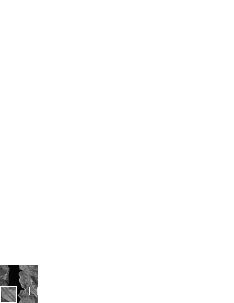
(a)

(b)

(c)

(d)

(e)

(f)

(g)

(h)

(i)

(j)

(k)

Figure 2: Denoising results for Jasper Ridge with the 131st band in Case 1. Upper row images are the restored images by each method. Lower row images are the absolute difference between the original image and each restored image (the range of the only observed noisy image in (b) is $[0,1]$). (a) Ground-truth. (b) Observed noisy image. (c) SSTV. (d) HSSTV1. (e) HSSTV2. (f) ${l_{0}\text{-}l_{1}\text{HTV}}$. (g) STV. (h) SSST. (i) LRTDTV. (j) TPTV. (k) ${\text{S}_{3}\text{TTV}}$ (ours).

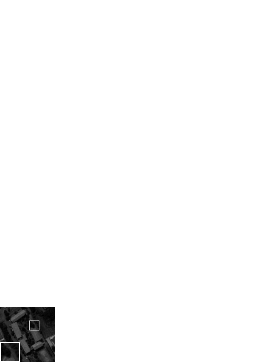
(a)

(b)

(c)

(d)

(e)

(f)

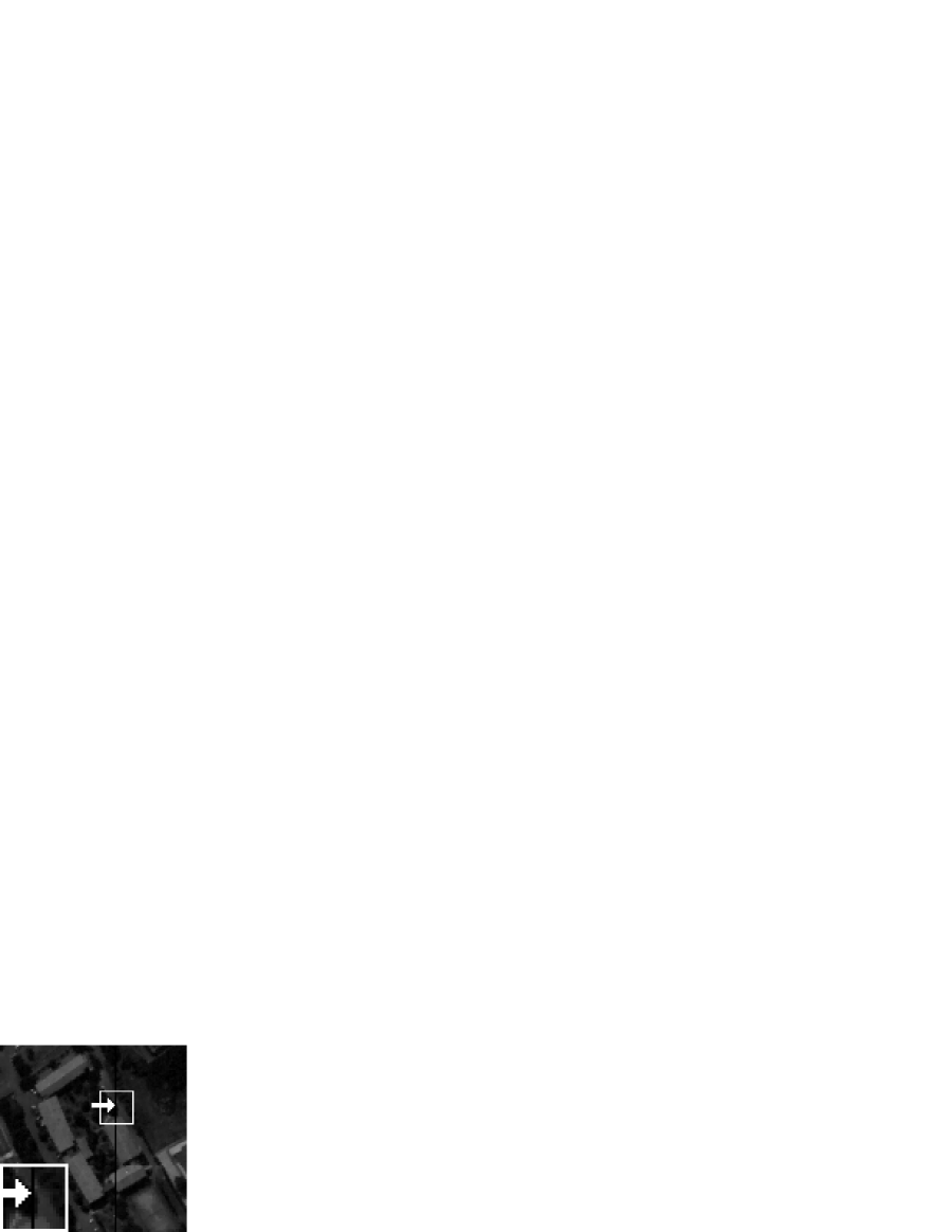
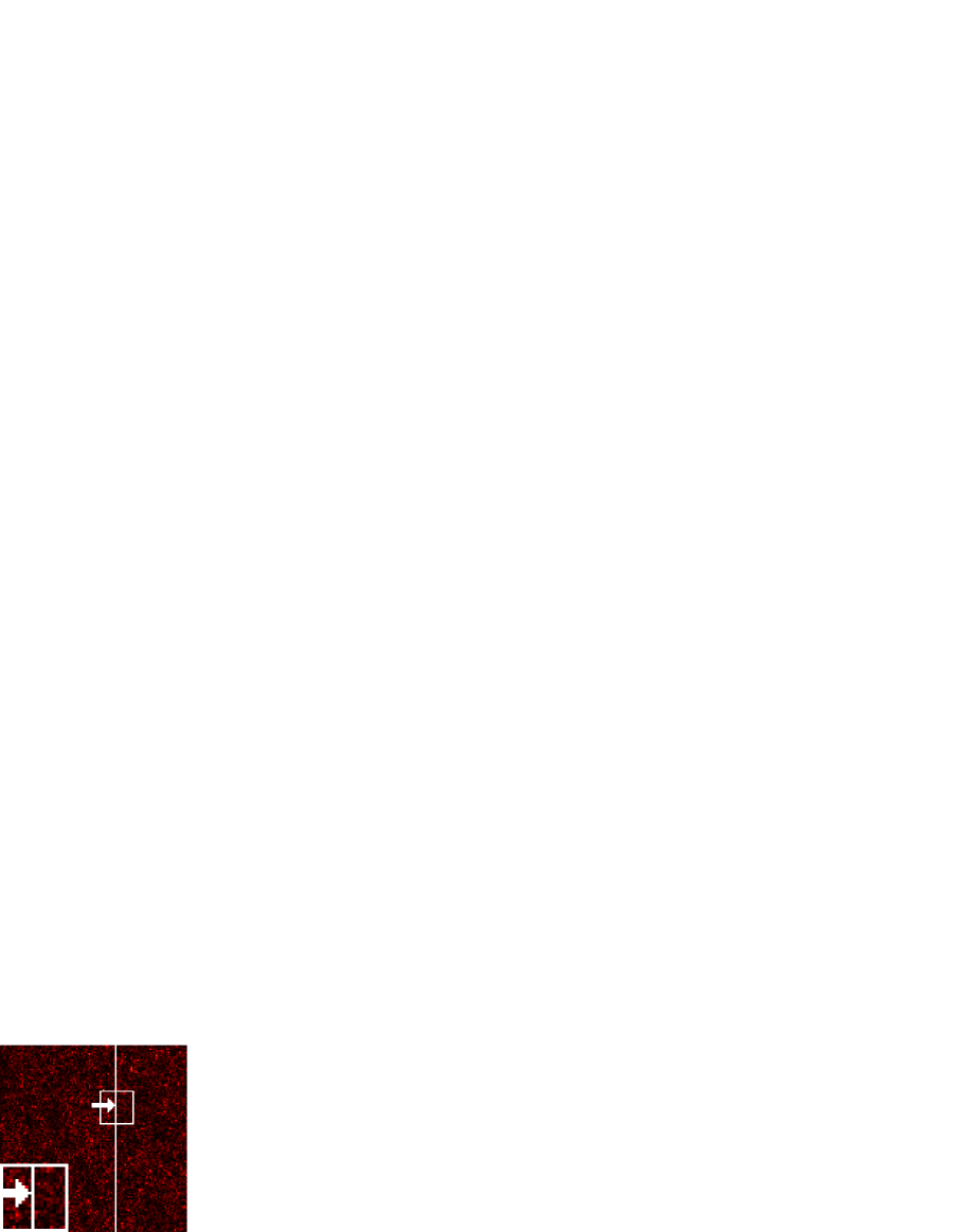
(g)

(h)

(i)

(j)

(k)

Figure 3: Denoising and destriping results for Pavia University with the 58th band in Case 3. Upper row images are the restored images by each method. Lower row images are the absolute difference between the original image and each restored image (the range of the only observed noisy image in (b) is $[0,1]$). (a) Ground-truth. (b) Observed noisy image. (c) SSTV. (d) HSSTV1. (e) HSSTV2. (f) ${l_{0}\text{-}l_{1}\text{HTV}}$. (g) STV. (h) SSST. (i) LRTDTV. (j) TPTV. (k) ${\text{S}_{3}\text{TTV}}$ (ours).

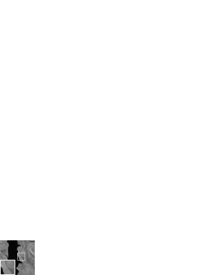
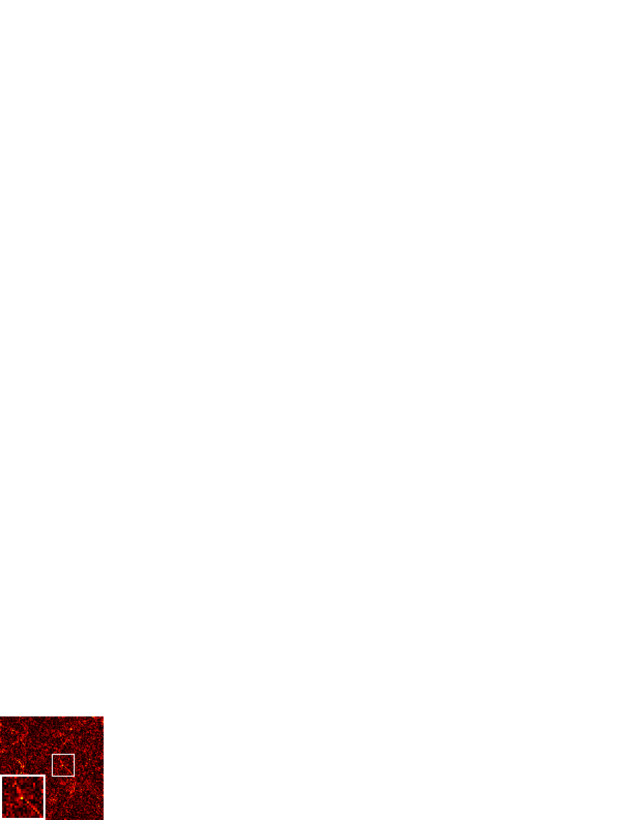
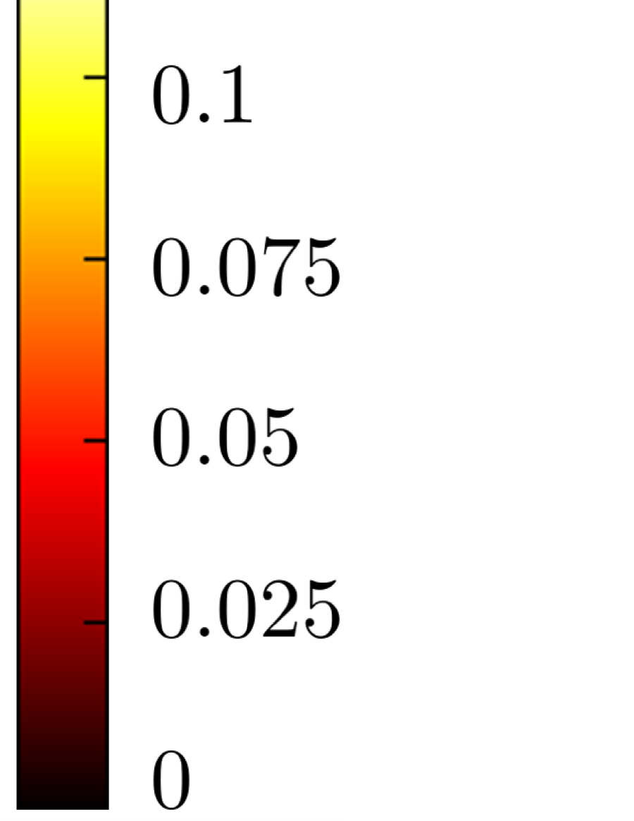
(a)

(b)

(c)

(d)

(e)

(f)

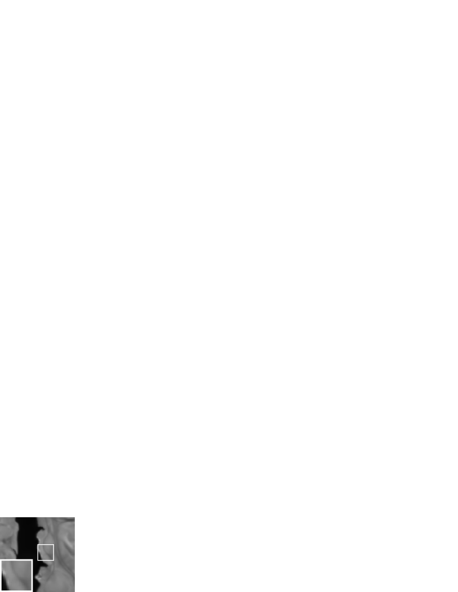
(g)

(h)

(i)

(j)

(k)

Figure 4: Denoising and destriping results for Jasper Ridge with the 59th band in Case 6. Upper row images are the restored images by each method. Lower row images are the absolute difference between the original image and each restored image (the range of the only observed noisy image in (b) is $[0,1]$). (a) Ground-truth. (b) Observed noisy image. (c) SSTV. (d) HSSTV1. (e) HSSTV2. (f) ${l_{0}\text{-}l_{1}\text{HTV}}$. (g) STV. (h) SSST. (i) LRTDTV. (j) TPTV. (k) ${\text{S}_{3}\text{TTV}}$ (ours).

We adopt two HS image datasets which have different structures information.

IV-A1 Jasper Ridge

This HS image was captured using an Airborne Visible/Infrared Imaging Spectrometer (AVIRIS) sensor in a rural area of California, USA. Jasper Ridge consists of a large river in the center and fine structure on the left and right. The resolution of the original data is $512\times 614$ pixels with 224 spectral bands per pixel. After removing several noisy bands and cropping the original data, we obtained the HS image with $100\times 100$ pixels and 198 bands.

IV-A2 Pavia University

This HS image was captured using a Reflective Optics System Imaging Spectrometer (ROSIS) sensor in Pavia, northern Italy. Pavia University consists of complex structures. The resolution of the original data is $610\times 610$ pixels with 103 spectral bands per pixel. After removing several noisy bands and cropping the original data, we obtained the HS image with $120\times 120$ pixels and 99 bands.

All the intensities of both HS images were normalized within the range $[0,1]$.

HS images are often degraded by a mixture of various types of noise in real-world scenarios. Thus, in the experiments, we consider the following six cases of noise contamination:

• The observed HS image is contaminated by white Gaussian noise with the standard deviation $\sigma=0.05$ and salt-and-pepper noise with the rate $p_{\mathbf{s}}=0.05$.

• The observed HS image is contaminated by white Gaussian noise with the standard deviation $\sigma=0.1$ and salt-and-pepper noise with the rate $p_{\mathbf{s}}=0.05$.

• The observed HS image is contaminated by white Gaussian noise with the standard deviation $\sigma=0.05$ and vertical stripe noise whose intensity is uniformly random in the range $[-0.5,0.5]$ with the rate $p_{\mathbf{t}}=0.05$.

• The observed HS image is contaminated by white Gaussian noise with the standard deviation $\sigma=0.1$ and vertical stripe noise whose intensity is uniformly random in the range $[-0.5,0.5]$ with the rate $p_{\mathbf{t}}=0.05$.

• The observed HS image is contaminated by white Gaussian noise with the standard deviation $\sigma=0.05$, salt-and-pepper noise with the rate $p_{\mathbf{s}}=0.05$, and vertical stripe noise whose intensity is uniformly random in the range $[-0.5,0.5]$ with the rate $p_{\mathbf{t}}=0.05$.

• The observed HS image is contaminated by white Gaussian noise with the standard deviation $\sigma=0.1$, salt-and-pepper noise with the rates $p_{\mathbf{s}}=0.05$, and vertical stripe noise whose intensity is uniformly random in the range $[-0.5,0.5]$ with the rates $p_{\mathbf{t}}=0.05$.

The block size of ${\text{S}_{3}\text{TTV}}$ was set to $10\times 10\times N_{3}$. The radii $\alpha$, $\beta$, and $\varepsilon$ were set as follows:

$$\alpha=\rho\tfrac{Np_{\mathbf{s}}}{2},\>\beta=\rho\tfrac{0.5Np_{\mathbf{t}}(1-p_{\mathbf{s}})}{2},\>\varepsilon=\rho\sqrt{\sigma^{2}N(1-p_{\mathbf{s}})},$$ (25)

where the parameter $\rho$ was set to $0.95$. The stopping criterion of Alg. 1 were set as follows:

$$\frac{\|\mathbf{u}^{(t+1)}-\mathbf{u}^{(t)}\|_{2}}{\|\mathbf{u}^{(t)}\|_{2}}<1.0\times 10^{-5}.$$ (26)

For the quantitative evaluation, we employed the mean peak signal-to-noise ratio (MPSNR):

$$\mathrm{MPSNR}=\frac{1}{N_{3}}\sum_{i=1}^{N_{3}}10\log_{10}\frac{N_{1}N_{2}}{\|\mathbf{u}_{i}-\bar{\mathbf{u}}_{i}\|_{2}^{2}},$$ (27)

and the mean structural similarity index (MSSIM) [47]:

$$\mathrm{MSSIM}=\frac{1}{N_{3}}\sum_{i=1}^{N_{3}}\mathrm{SSIM}(\mathbf{u}_{i},\bar{\mathbf{u}}_{i}),$$ (28)

where $\mathbf{u}_{i}$ and $\bar{\mathbf{u}}_{i}$ are the $i$-th band of the ground true HS image $\mathbf{u}$ and the estimated HS image $\bar{\mathbf{u}}$, respectively. Generally, higher MPSNR and MSSIM values are corresponding to better denoising performances.

IV-A1 Quantitative Comparison

Tables II and III show MPSNRs and MSSIMs in the experiments on the HS image contaminated with simulated noise. The best and second best results are highlighted in bold and underlined, respectively. STV is worse in all cases. The SSST results show high performance in stripe noise removal, especially in Case 4 for MSSIMs. However, its effectiveness is degraded when the HS image is contaminated with sparse noise. As for LRTDTV, its performance drops when stripe noise is included. The SSTV-type methods, including SSTV, HSSTV1, HSSTV2, and ${l_{0}\text{-}l_{1}\text{HTV}}$, outperform STV, SSST, and LRTDTV. Among the SSTV-type methods, HSSTV1 performs better for MSSIMs of Pavia University. TPTV yields overall higher MPSNRs and MSSIMs than the other existing methods, most notably for the MSSIMs of Jasper Ridge. However, in Cases 3 and 4, MPSNRs of TPTV are worse than those of the SSTV-based methods. On the other hand, ${\text{S}_{3}\text{TTV}}$ achieves the best MPSNRs in most cases, and in the two exceptions, it still ranks second highest. Moreover, ${\text{S}_{3}\text{TTV}}$ shows a high overall performance independent of the HS images.

IV-A2 Visual Quality Comparison

Figs. 2-4 show the results of HS image denoising and destriping. The lower row images are the absolute difference between the original image and each restored image.

Fig. 2 shows the denoising results for Jasper Ridge in Case 1, i.e. under contamination by both Gaussian and sparse noise. In the restored images by STV and SSST in (g) and (h), spatial over-smoothing occurs because the nuclear norm of the “first-order” differences is directly suppressed. The restored images by SSTV-based methods (SSTV, HSSTV1, HSSTV2, and ${l_{0}\text{-}l_{1}\text{HTV}}$) and LRTDTV in (c), (d), (e), (f), and (i) have more structure than those by STV and SSST. However, edges and textures appear in these difference images between the ground-truth and these restored images. Especially in the enlarged images, the edges of the road are clearly visible. In other words, these detailed structures are lost in the restored images. On the other hand, as shown in (j) and (k), TPTV and ${\text{S}_{3}\text{TTV}}$ achieve higher restoration performance than the methods presented above.

Fig. 3 shows the denoising results for Pavia University in Case 3, i.e. under contamination by both Gaussian and stripe noise. As indicated by the rightward arrow in (j), the black line exists in the restored HS image by TPTV. More stripe noise remains in the restored HS image by LRTDTV, including that indicated by the leftward arrows. These occur due to the mischaracterization of stripe noise. As for other methods, including our method, stripe noise is adequately removed. This is thanks to the second and third constraints in Eq. (13) that characterize stripe noise. Furthermore, the methods that mainly use the second-order spatio-spectral differences, i.e., SSTV, HSSTV1, HSSTV2, ${l_{0}\text{-}l_{1}\text{HTV}}$, and our method fully recover HS images without over-smoothing.

Fig. 4 shows the denoising results for Jasper Ridge in Case 6, which is the most contaminated case with Gaussian, sparse, and stripe noise. For STV and SSST in (g) and (h), no stripe noise remains in the restored images, but edges and textures are lost along with the noise. SSTV, HSSTV1, HSSTV2, and ${l_{0}\text{-}l_{1}\text{HTV}}$ in (c), (d), (e), and (f) restore edges and textures more clearly than STV and SSST, but still remove some edges and textures (see the difference images in (c), (d), (e), and (f) of Fig. 4). This would be due to the fact that these methods suffer more from the limitation of referring only to adjacent pixels/bands. LRTDTV and TPTV almost recover edges and textures in the restored images of (i) and (j), but as in Case 3, stripe noise remains at the positions indicated by the arrows. On the other hand, the difference image of ${\text{S}_{3}\text{TTV}}$ in (k) is closer to black than the other methods. Furthermore, no edges or textures are visible in the enlarged image. These suggest that ${\text{S}_{3}\text{TTV}}$ removes Gaussian, sparse, and stripe noise most effectively and recovers edges and textures with the highest accuracy.

IV-B Real HS Image Experiment

(b)

(c)

(d)

(e)

(f)

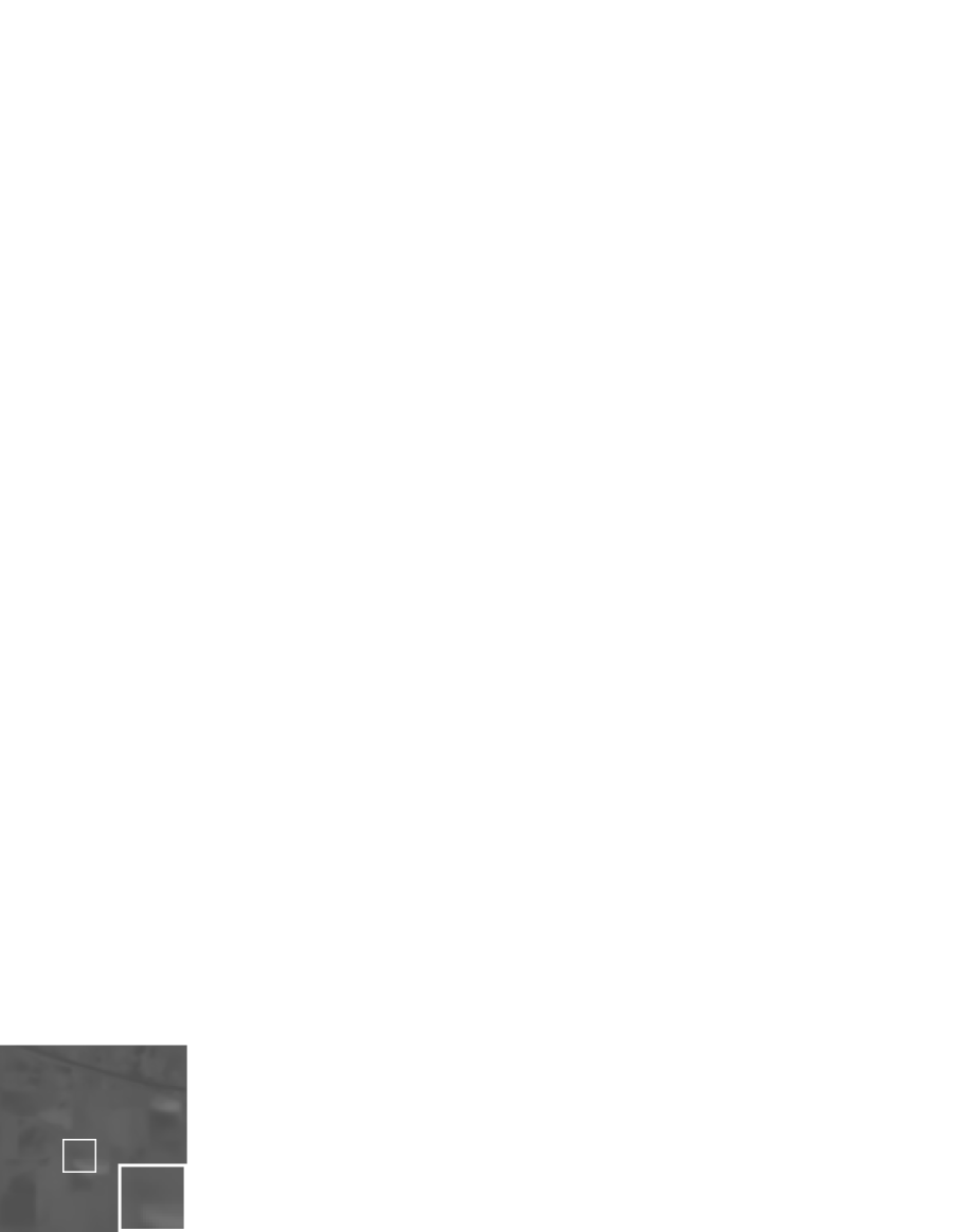
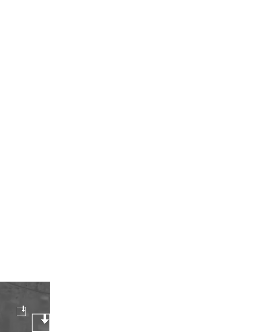
(g)

(h)

(i)

(j)

(k)

Figure 5: Denoising and destriping results for Indian Pines with the 88th band, multiplied by 1.5 for visibility. (b) Observed noisy image. (c) SSTV. (d) HSSTV1. (e) HSSTV2. (f) ${l_{0}\text{-}l_{1}\text{HTV}}$. (g) STV. (h) SSST. (i) LRTDTV. (j) TPTV. (k) ${\text{S}_{3}\text{TTV}}$ (ours).

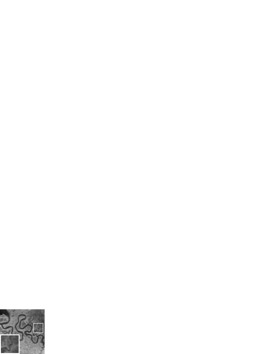
(b)

(c)

(d)

(e)

(f)

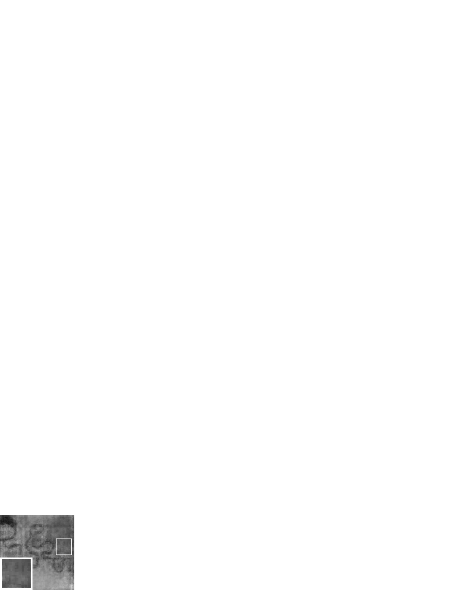
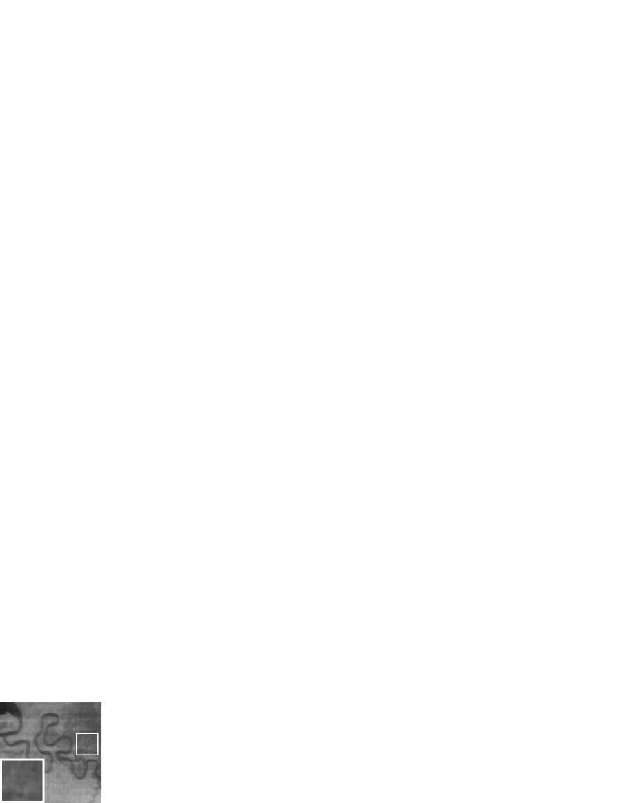
(g)

(h)

(i)

(j)

(k)

Figure 6: Denoising and destriping results for Suwannee with the 197th band. (b) Observed noisy image. (c) SSTV. (d) HSSTV1. (e) HSSTV2. (f) ${l_{0}\text{-}l_{1}\text{HTV}}$. (g) STV. (h) SSST. (i) LRTDTV. (j) TPTV. (k) ${\text{S}_{3}\text{TTV}}$ (ours).

We employed the following two datasets:

IV-B1 Indian Pines

This HS image was captured using the AVIRIS sensor over the Indian Pines test site in North-western Indiana. The resolution of the original data is $145\times 145$ pixels, and each pixel has spectral information with 224 bands ranging from 400 nm to 2500 nm. After removing several noisy bands and cropping the original data, we obtained the HS image with $120\times 120$ pixels and 198 bands.

IV-B2 Suwannee

This HS image was captured using a SpecTIR sensor over the Suwannee River Basin in Florida, USA. The resolution of the original HS image is $1200\times 320$ pixels, and each pixel has spectral information with 360 bands ranging from 400 nm to 2500 nm. We cropped the HS image to $100\times 100$ pixels and 360 bands.

All the intensities of both HS images were normalized within the range $[0,1]$. The block size of ${\text{S}_{3}\text{TTV}}$ was set to $10\times 10\times N_{3}$. For the radii $\alpha$, $\beta$, and $\varepsilon$, we adjusted them to appropriate values after empirically estimating the intensity of the noise in the real HS image. Specifically, for the Indian Pines, $\alpha$, $\beta$, and $\varepsilon$ were set to 200, 100, and 30, respectively, and for Suwannee, they were set to 800, 5000, and 100, respectively. The stopping criterion of Alg. 1 were set as follows:

$$\frac{\|\mathbf{u}^{(t+1)}-\mathbf{u}^{(t)}\|_{2}}{\|\mathbf{u}^{(t)}\|_{2}}<1.0\times 10^{-5}.$$ (29)

Since no reference clean HS image is available, we compare the denoising performance using visual results. Fig. 5 shows the HS image denoising and destriping results for Indian Pines. HSSTV1, STV, and SSST cause over-smoothing in the restored images of (d), (g), and (h). For LRTDTV and TPTV in (i) and (j), noise remains in the restored images. On the other hand, SSTV, HSSTV2, ${l_{0}\text{-}l_{1}\text{HTV}}$, and ${\text{S}_{3}\text{TTV}}$ achieve sufficient noise removal while preserving edges and textures. This is due to the characterization of the spatial similarity between adjacent bands of HS images using the second-order spatio-spectral differences. In the enlarged area, SSTV, HSSTV2, and ${\text{S}_{3}\text{TTV}}$ restore the edges indicated by the arrows, while ${l_{0}\text{-}l_{1}\text{HTV}}$ loses them.

Fig. 6 shows the HS image denoising and destriping results for Suwannee. The restored images by STV, LRTDTV, and TPTV in (g), (i), and (j) still retain vertical stripe noise. For LRTDTV and TPTV, this is due to the limitation of stripe noise removal, similar to the results seen in the simulation experiments of Figs. 3 and 4. In the case of STV, its regularization method, which mainly captures the spatial piecewise-smoothness in HS images, is insufficient to separate the HS image and vertically smooth stripe noise. On the other hand, SSTV, HSSTV1, HSSTV2, ${l_{0}\text{-}l_{1}\text{HTV}}$, SSST, and ${\text{S}_{3}\text{TTV}}$ sufficiently remove stripe noise. This indicates that the second and third constraints characterizing stripe noise in Eq. (13) are effective for real stripe noise. However, the edges of the restored images by HSSTV1 and SSST in (d) and (h) are smoothed in the enlarged areas. Unlike these methods, SSTV, HSSTV2, ${l_{0}\text{-}l_{1}\text{HTV}}$, and the proposed method, ${\text{S}_{3}\text{TTV}}$, achieve the preservation of the narrow river structure while removing noise.

IV-C Summary

We summarize the insights from the experiments as follows.

1. The simulated HS image data experiments demonstrate that ${\text{S}_{3}\text{TTV}}$ outperforms existing methods in removing mixed noise while preserving edges and textures in HS images with high accuracy. This indicates that ${\text{S}_{3}\text{TTV}}$ is the most effective in removing mixed noise.

2. The real HS image data experiments show that ${\text{S}_{3}\text{TTV}}$ has high performance even when observed HS images are degraded by real noise.

V Conclusion

In this paper, we have proposed a new regularization method, named ${\text{S}_{3}\text{TTV}}$, for denoising and destriping of HS images. ${\text{S}_{3}\text{TTV}}$ is defined as the sum of the nuclear norms of matrices consisting of second-order spatio-spectral differences in small spectral blocks, which fully captures the spatial piecewise-smoothness, the spatial similarity between adjacent bands, and the spectral correlation across all bands of HS images. We have formulated the denoising and destriping problem as a constrained convex optimization problem including ${\text{S}_{3}\text{TTV}}$, and developed the optimization algorithm based on P-PDS. Experiments on HS images with simulated or real noise have demonstrated the superiority of ${\text{S}_{3}\text{TTV}}$ over existing methods. ${\text{S}_{3}\text{TTV}}$ will have a strong impact on the field of remote sensing, including applications using HS images taken in highly degraded measurement environments.

Shingo Takemoto (S’22) received a B.E. degree and M.E. degree in Information and Computer Sciences in 2021 from Sophia University and in 2023 from Tokyo Institute of Technology, respectively. He is currently pursuing an Ph.D. degree at the Department of Computer Science in the Tokyo Institute of Technology. His current research interests are in signal and image processing and optimization theory. Mr. Takemoto received the Student Award from IEEE SPS Tokyo Joint Chapter in 2022.

Shunsuke Ono (S’11–M’15–SM’23) received a B.E. degree in Computer Science in 2010 and M.E. and Ph.D. degrees in Communications and Computer Engineering in 2012 and 2014 from the Tokyo Institute of Technology, respectively. From April 2012 to September 2014, he was a Research Fellow (DC1) of the Japan Society for the Promotion of Science (JSPS). He is currently an Associate Professor in the Department of Computer Science, School of Computing, Tokyo Institute of Technology. From October 2016 to March 2020 and from October 2021 to present, he was/is a Researcher of Precursory Research for Embryonic Science and Technology (PRESTO), Japan Science and Technology Agency (JST), Tokyo, Japan. His research interests include signal processing, image analysis, remote sensing, mathematical optimization, and data science. Dr. Ono received the Young Researchers’ Award and the Excellent Paper Award from the IEICE in 2013 and 2014, respectively, the Outstanding Student Journal Paper Award and the Young Author Best Paper Award from the IEEE SPS Japan Chapter in 2014 and 2020, respectively, the Funai Research Award from the Funai Foundation in 2017, the Ando Incentive Prize from the Foundation of Ando Laboratory in 2021, the Young Scientists’ Award from MEXT in 2022, and the Outstanding Editorial Board Member Award from IEEE SPS in 2023. He has been an Associate Editor of IEEE TRANSACTIONS ON SIGNAL AND INFORMATION PROCESSING OVER NETWORKS since 2019.

References

- [1] M. Borengasser, W. S Hungate, and R. Watkins, Hyperspectral remote sensing: principles and applications, CRC press, 2007.
- [2] H. Grahn and P. Geladi, Techniques and applications of hyperspectral image analysis, John Wiley & Sons, 2007.
- [3] P. S. Thenkabail, J. G. Lyon, and A. Huete, Hyperspectral remote sensing of vegetation, CRC press, 2016.
- [4] B. Lu, P. D. Dao, J. Liu, Y. He, and J. Shang, “Recent advances of hyperspectral imaging technology and applications in agriculture,” Remote Sens., vol. 12, no. 16, pp. 2659, 2020.
- [5] H. Shen, X. Li, Q. Cheng, C. Zeng, G. Yang, H. Li, and L. Zhang, “Missing information reconstruction of remote sensing data: A technical review,” IEEE Geosci. Remote Sens. Mag., vol. 3, no. 3, pp. 61–85, 2015.
- [6] B. Rasti, P. Scheunders, P. Ghamisi, G. Licciardi, and J. Chanussot, “Noise reduction in hyperspectral imagery: Overview and application,” Remote Sens., vol. 10, no. 3, 2018.
- [7] H. Shen, M. Jiang, J. Li, C. Zhou, Q. Yuan, and L. Zhang, “Coupling model- and data-driven methods for remote sensing image restoration and fusion: Improving physical interpretability,” IEEE Geosci. Remote Sens. Mag., vol. 10, no. 2, pp. 231–249, 2022.
- [8] J. M. Bioucas-Dias, A. Plaza, N. Dobigeon, M. Parente, Q. Du, P. Gader, and J. Chanussot, “Hyperspectral unmixing overview: Geometrical, statistical, and sparse regression-based approaches,” IEEE J. Sel. Topics Appl. Earth Observ. Remote Sens., vol. 5, no. 2, pp. 354–379, 2012.
- [9] W. Ma, J. M. Bioucas-Dias, T. Chan, N. Gillis, P. Gader, A. J. Plaza, A. Ambikapathi, and C. Chi, “A signal processing perspective on hyperspectral unmixing: Insights from remote sensing,” IEEE Signal Process. Mag., vol. 31, no. 1, pp. 67–81, 2014.
- [10] P. Ghamisi, J. Plaza, Y. Chen, J. Li, and A. J Plaza, “Advanced spectral classifiers for hypersfnopectral images: A review,” IEEE Geosci. Remote Sens. Mag., vol. 5, no. 1, pp. 8–32, 2017.
- [11] S. Li, W. Song, L. Fang, Y. Chen, P. Ghamisi, and J. A. Benediktsson, “Deep learning for hyperspectral image classification: An overview,” IEEE Trans. Geosci. Remote Sens., vol. 57, no. 9, pp. 6690–6709, 2019.
- [12] N. Audebert, B. L. Saux, and S. Lefevre, “Deep learning for classification of hyperspectral data: A comparative review,” IEEE Geosci. Remote Sens. Mag., vol. 7, no. 2, pp. 159–173, 2019.
- [13] S. Matteoli, M. Diani, and J. Theiler, “An overview of background modeling for detection of targets and anomalies in hyperspectral remotely sensed imagery,” IEEE J. Sel. Topics Appl. Earth Observ. Remote Sens., vol. 7, no. 6, pp. 2317–2336, 2014.
- [14] H. Su, Z. Wu, H. Zhang, and Q. Du, “Hyperspectral anomaly detection: A survey,” IEEE Geosci. Remote Sens. Mag., vol. 10, no. 1, pp. 64–90, 2022.
- [15] L. I. Rudin, S. Osher, and E. Fatemi, “Nonlinear total variation based noise removal algorithms,” Physica D: Nonlinear Phenomena, vol. 60, no. 1, pp. 259–268, 1992.
- [16] X. Bresson and T. F. Chan, “Fast dual minimization of the vectorial total variation norm and applications to color image processing,” Inverse problems imag., vol. 2, no. 4, pp. 455–484, 2008.
- [17] Q. Yuan, L. Zhang, and H. Shen, “Hyperspectral image denoising employing a spectral–spatial adaptive total variation model,” IEEE Trans. Geosci. Remote Sens., vol. 50, no. 10, pp. 3660–3677, 2012.
- [18] Y. Chang, L. Yan, H. Fang, and C. Luo, “Anisotropic spectral-spatial total variation model for multispectral remote sensing image destriping,” IEEE Trans. Image Process., vol. 24, no. 6, pp. 1852–1866, 2015.
- [19] W. He, H. Zhang, L. Zhang, and H. Shen, “Total-variation-regularized low-rank matrix factorization for hyperspectral image restoration,” IEEE Trans. Geosci. Remote Sens., vol. 54, no. 1, pp. 178–188, 2016.
- [20] Y. Wang, J. Peng, Q. Zhao, Y. Leung, X. Zhao, and D. Meng, “Hyperspectral image restoration via total variation regularized low-rank tensor decomposition,” IEEE J. Sel. Topics Appl. Earth Observ. Remote Sens., vol. 11, no. 4, pp. 1227–1243, 2018.
- [21] Y. Chen, W. Cao, L. Pang, J. Peng, and X. Cao, “Hyperspectral image denoising via texture-preserved total variation regularizer,” IEEE Trans. Geosci. Remote Sens., vol. 61, pp. 1–14, 2023.
- [22] H. K. Aggarwal and A. Majumdar, “Hyperspectral image denoising using spatio-spectral total variation,” IEEE Geosci. Remote Sens. Lett., vol. 13, no. 3, pp. 442–446, 2016.
- [23] H. Fan, C. Li, Y. Guo, G. Kuang, and J. Ma, “Spatial–spectral total variation regularized low-rank tensor decomposition for hyperspectral image denoising,” IEEE Trans. Geosci. Remote Sens., vol. 56, no. 10, pp. 6196–6213, 2018.
- [24] T. Ince, “Hyperspectral image denoising using group low-rank and spatial-spectral total variation,” IEEE Access, vol. 7, pp. 52095–52109, 2019.
- [25] S. Takeyama, S. Ono, and I. Kumazawa, “A constrained convex optimization approach to hyperspectral image restoration with hybrid spatio-spectral regularization,” Remote Sens., vol. 12, no. 21, 2020.
- [26] M. Wang, Q. Wang, J. Chanussot, and D. Hong, “- hybrid total variation regularization and its applications on hyperspectral image mixed noise removal and compressed sensing,” IEEE Trans. Geosci. Remote Sens., vol. 59, no. 9, pp. 7695–7710, 2021.
- [27] S. Takemoto, K. Naganuma, and S. Ono, “Graph spatio-spectral total variation model for hyperspectral image denoising,” IEEE Geosci. Remote Sens. Lett., vol. 19, pp. 1–5, 2022.
- [28] S. Ono, “ gradient projection,” IEEE Trans. Image Process., vol. 26, no. 4, pp. 1554–1564, 2017.
- [29] S. Lefkimmiatis, A. Roussos, P. Maragos, and M. Unser, “Structure tensor total variation,” SIAM J. Imag. Sci., vol. 8, no. 2, pp. 1090–1122, 2015.
- [30] Z. Wu, Q. Wang, J. Jin, and Y. Shen, “Structure tensor total variation-regularized weighted nuclear norm minimization for hyperspectral image mixed denoising,” Signal Process., vol. 131, pp. 202–219, 2017.
- [31] S. Ono, K. Shirai, and M. Okuda, “Vectorial total variation based on arranged structure tensor for multichannel image restoration,” in Proc. IEEE Int. Conf. Acoust., Speech, Signal Process. (ICASSP), 2016, pp. 4528–4532.
- [32] R. Kurihara, S. Ono, K. Shirai, and M. Okuda, “Hyperspectral image restoration based on spatio-spectral structure tensor regularization,” in Proc. Eur. Signal Process. Conf. (EUSIPCO), 2017, pp. 488–492.
- [33] M. V. Afonso, J. M. Bioucas-Dias, and M. Figueiredo, “An augmented lagrangian approach to the constrained optimization formulation of imaging inverse problems,” IEEE Trans. Image Process., vol. 20, no. 3, pp. 681–695, 2011.
- [34] G. Chierchia, N. Pustelnik, J.-C. Pesquet, and B. Pesquet-Popescu, “Epigraphical projection and proximal tools for solving constrained convex optimization problems,” Signal Image Video Process., vol. 9, no. 8, pp. 1737–1749, 2015.
- [35] S. Ono and I. Yamada, “Signal recovery with certain involved convex data-fidelity constraints,” IEEE Trans. Signal Process., vol. 63, no. 22, pp. 6149–6163, 2015.
- [36] S. Ono, “Primal-dual plug-and-play image restoration,” IEEE Signal Process. Lett., vol. 24, no. 8, pp. 1108–1112, 2017.
- [37] S. Ono, “Efficient constrained signal reconstruction by randomized epigraphical projection,” in Proc. IEEE Int. Conf. Acoust., Speech, Signal Process., (ICASSP), 2019, pp. 4993–4997.
- [38] K. Naganuma and S. Ono, “A general destriping framework for remote sensing images using flatness constraint,” IEEE Trans. Geosci. Remote Sens., vol. 60, pp. 1–16, 2022.
- [39] T. Pock and A. Chambolle, “Diagonal preconditioning for first order primal-dual algorithms in convex optimization,” in Proc. IEEE Int. Conf. Comput. Vis. (ICCV), 2011, pp. 1762–1769.
- [40] S. Boyd, N. Parikh, E. Chu, B. Peleato, and J. Eckstein, “Distributed optimization and statistical learning via the alternating direction method of multipliers,” Found. Trends Mach. Learn., vol. 3, no. 1, pp. 1–122, 2011.
- [41] A. Chambolle and T. Pock, “A first-order primal-dual algorithm for convex problems with applications to imaging,” J. Math. Imag. Vis., vol. 40, no. 1, pp. 120–145, 2011.
- [42] L. Condat, “A primal–dual splitting method for convex optimization involving lipschitzian, proximable and linear composite terms,” J. Optim. Theory Appl., vol. 158, no. 2, pp. 460–479, 2013.
- [43] K Naganuma and S Ono, “Variable-wise diagonal preconditioning for primal-dual splitting: Design and applications,” IEEE Trans. Signal Process., vol. 71, pp. 3281–3295, 2023.
- [44] S. Takemoto and S. Ono, “Enhancing spatio-spectral regularization by structure tensor modeling for hyperspectral image denoising,” in Proc. IEEE Int. Conf. Acoust., Speech, Signal Process. (ICASSP), 2023, pp. 1–5.
- [45] P. L. Combettes and N. N. Reyes, “Moreau’s decomposition in banach spaces,” Math. Program., vol. 139, no. 1, pp. 103–114, 2013.
- [46] L. Condat, “Fast projection onto the simplex and the ball,” Math. Program., vol. 158, no. 1, pp. 575–585, 2016.
- [47] Z. Wang, A.C. Bovik, H.R. Sheikh, and E.P. Simoncelli, “Image quality assessment: from error visibility to structural similarity,” IEEE Trans. Image Process., vol. 13, no. 4, pp. 600–612, 2004.