Optimistic Online Non-stochastic Control via FTRL
Abstract
This paper brings the concept of “optimism” to the new and promising framework of online Non-stochastic Control (NSC). Namely, we study how can NSC benefit from a prediction oracle of unknown quality responsible for forecasting future costs. The posed problem is first reduced to an optimistic learning with delayed feedback problem, which is handled through the Optimistic Follow the Regularized Leader (OFTRL) algorithmic family. This reduction enables the design of OptFTRL-C, the first Disturbance Action Controller (DAC) with optimistic policy regret bounds. These new bounds are commensurate with the oracle’s accuracy, ranging from for perfect predictions to the order-optimal even when all predictions fail. By addressing the challenge of incorporating untrusted predictions into control systems, our work contributes to the advancement of the NSC framework and paves the way towards effective and robust learning-based controllers.
I Introduction
We study the NSC framework originally introduced in [1]: Consider a time-slotted dynamical system where at each time slot, the controller observes the system state and decides an action which then induces a cost , and causes a transition to a new state . Note that the cost and the new state are revealed to the controller after it commits its action. Similar to [1], we study Linear Time Invariant (LTI) systems where the state transition is parameterized by matrices , and a disturbance vector :
| (1) |
can be arbitrarily set by an adversary, and we only restrict it to be upper-bounded, i.e., . Similarly, the adversary is allowed to select any -Lipschitz convex cost function at each slot. Since neither the cost nor disturbances are confined to follow a fixed and/or known distribution, the control problem is “Non-stochastic”.
The controller (or learner) aims to find a (possibly time-varying) policy that maps states to actions, , from a given policy class , such that the cost trajectory is as small as possible. To quantify the learner’s performance, we employ the policy regret metric, as presented in [2]. Intuitively, the policy regret measures the accumulated differences between the cost incurred by the learner’s policy, and that of a stationary unknown cost-minimizing policy designed with access to all future cost functions and disturbances:
| (2) |
where is the counterfactual state-action sequence that would have emerged under the benchmark policy, whereas is the actual state-action sequence that emerged from following possibly different policies by the learner. A sub-linear regret means that the cost endured by the learner will converge to that of the optimal unknown policy at the same sub-linear rate, i.e., as . Note that the benchmark depends on the actual witnessed costs and disturbances, encoding a stronger concept of “adaptability” unlike the pessimistic controllers, which assume worst case costs [3]. Remarkably, the Gradient Perturbation Controller (GPC) achieves regret, which is order optimal, and was shown to deliver superior performance to the more conventional controllers [1].
In contrast to the typical NSC framework, here we consider the existence of a prediction oracle. This oracle provides the learner, before committing to the action , with a forecast for the as-yet-unobserved cost functions for a specific horizon of slots. We denote the oracle’s outcome as . Notably, the predictions themselves can be influenced by the adversary, meaning that no assumptions on the oracle’s accuracy are made; the forecasted parameters may either deviate arbitrarily from the truth, or be actually accurate in the best case.
The motivation for this addition on the NSC framework stems from the abundance of machine learning forecasting models, which provide high potential improvement if they are adequately accurate. The effect of such predictions on the classical regret metric (not the policy regret) has been studied in the literature of optimistic online learning, where the ultimate objective is to provide regret guarantees that scale with the accuracy of predictions while always staying sub-linear. Namely: when all predictions are accurate and in all cases. That is, we are assured of reaching the performance of the benchmark policy, yet at a significantly improved rate when predictions happen to be precise. Hence, optimistic online learning represents a highly desirable combination of the best of both worlds: optimal worst-case guarantees with achievable best case guarantees. In fact, optimistic learning algorithms have been attracting considerable attention as the driving force behind recent state-of-the-art results in online constrained optimization [4], online discrete optimization [5], online sub-modular optimization [6], and online fairness [7] to name a few.
Unfortunately, such optimistic algorithms are yet to find their way to online NSC. This might be surprising given that previous NSC results were obtained through a streamlined reduction to the standard Online Convex Optimization (OCO) framework [8]. Hence, one might anticipate that optimistic NSC algorithms can be derived using a similar approach. Interestingly, this is not the case. Combining optimistic learning and NSC poses unique challenges for both frameworks. First, existing optimistic learning algorithms do not consider cost functions with memory and hence cannot handle states. Particularly, these algorithms update their regularizers at each time slot based on the prediction accuracy of the preceding slot’s cost [9, 10]. However, in stateful systems, an action made at will have an effect that spans across all slots until , and thus uses predictions for all these slots. Since the accuracy of such multi-step predictions is not available until , we cannot update the regularizer in the same standard way. Second, the guarantee of NSC is established via a reduction to the OCO with Memory (OCO-M) framework [11], which in turn is reduced to the standard OCO [12] via the concept of slowly moving decision variables [1, Thm. 4.6] [11, Thm. 3.1]. This later reduction cannot be utilized in optimistic learning where accurate predictions lead to little or no regularization, driving consecutive decisions of the optimistic algorithm to vary arbitrarily (up to the decision set diameter) [10, Sec ], [13, Sec ].
This paper tackles exactly these challenges and aims to answer the question: is it possible to design an online learning algorithm whose policy regret is commensurate with the accuracy of an exogenous prediction oracle, while always staying sub-linear? Our paper answers this positively and builds upon recent advances in online learning, introducing, to our knowledge, the first optimistic controller for NSC.
We achieve such optimistic guarantees by departing from the standard analysis approach of reducing the learner’s non-stationary policy to a stationary one [1, 14, 15], and instead directly analyzing the non-stationary policy. Specifically, to address the first challenge, we demonstrate that the additive separability of the linearized costs allows expressing the costs as a sum of memoryless but delayed functions of each of the decision variables. Next, to tackle the second challenge, we analyze the performance of each decision variable separately via an alternative reduction to the framework of “optimism with delay” [16]. Nonetheless, we customize this later framework with a specific “hint” design that exploits the structure of NSC where the cost is indeed delayed but still gradually being revealed at each step, leading to tighter bounds. We make these intuition-focused points concrete in our upcoming analysis.
The main contribution is designing the first optimistic controller with policy regret that scales from to , depending on the predictions’ accuracy. The methodology is based on a new perspective on stateful systems as systems with delayed feedback, for which we build upon recent results on delay and optimism. The next section reviews the related works. Sec. III provides the necessary background for our new algorithm, OptFTRL-C, introduced in Section IV. We then present numerical examples in Sec. V and conclude.
II Related Work
The NSC problem was initiated in the seminal work of [1], which introduced the first controller with sub-linear policy regret for dynamical systems, generalizing the classical control problem to adversarial convex costs functions and adversarial disturbances. These results were further refined for strongly convex functions [17, 18, 19]; and systems where the actions are subject to fixed or adversarially-changing constraints [20, 21]. Follow-up works also looked at the NSC problem under more general assumptions on the system matrices, including unknown [2], systems with bandit feedback [22], and time-varying systems [23]. Expectedly, the regret bounds deteriorate in these cases, e.g., becoming for unknown systems and for systems with bandit feedback. Efficiency is also investigated in [15] with projection-free methods. Going beyond the typical bounds in terms of , [24] introduced an adaptive FTRL based controller whose bound is proportional to the witnessed costs and perturbations: instead of , where depends on the witnessed costs and perturbations. These works do not consider the existence of an untrusted prediction oracle, as the model adopted here.
The NSC framework was also investigated using other metrics such as dynamic regret [14], adaptive regret [25], and competitive ratio [26, 27]. For dynamic and adaptive regret, methods with static regret guarantees, as discussed here, are used as building blocks for “meta” algorithms with static/adaptive guarantees [23, 28]. For competitive ratio, it was demonstrated in [29] that a regret guarantee against the optimal DAC policy automatically implies a competitive ratio with an additive sub-linear term. Hence, the presented algorithm is still highly relevant even for other metrics.
Our work is also related to the robust MPC literature [30, 31], where (possibly inaccurate) predictions are used. However, the main difference is that while our algorithm is robust to bad predictions, it is not designed based on them. Specifically, our benchmark policy changes when worst case costs and predictions are not witnessed (as dictated by the regret metric). A newer line of research studies the MPC-style algorithms under the regret metric [32, 33]. Perfect predictions are assumed in [32], whose bound was later generalized in [33] with parameterized predictions error. While these works do not confine their policy class (i.e., directly optimizing ), their regret is linearly dependent on the prediction error, which renders them suffer linear regret in the worst case scenario.
Optimism is an extension to the OCO framework that allows incorporating predictions of future costs without having the regret bound linearly depend on their quality. The optimistic learning framework, in its current prevalent form, originated in [9] where an Online Mirror Descent (OMD) algorithm was presented. Thereafter, optimism was studied under another equivalent111see [34, Sec. 6] for a discussion on the link between OMD and FTRL. framework (FTRL). Optimistic FTRL (OFTRL) has since undergone multiple improvements [13, 35] and we refer the reader to [36, Sec. 7.12] for comprehensive overview. Only recently, a close connection between delay and optimism emerged [16], a development we leverage in our current analysis of the NSC framework.
While optimistic learning has been studied for stochastic predictions [37, 38], and adversarial predictions [10, 5], these findings have not been applied to dynamical systems. In dynamical systems, the study of predictions is limited to either perfect predictions [39, 40], or fixed quadratic (thus, strongly convex) cost functions [41, 42, 43]. Our paper contributes towards filling this gap. Predictions may also be viewed via the lens of “context” [44] in the different problem of stochastic MDPs with finite state and action space. Lastly, the previous works of [43, 42] consider that the full predictions are provided a priori, meaning that the learner cannot benefit from updated (and possibly more accurate) predictions. Like MPC, we drop this assumption and allow the learner to use the most recent available predictions.
III Preliminaries
Notation. We denote scalars by small letters, vectors by bold small letters, and matrices by capital letters. Time indexing is done via a subscript. We denote by the set . denotes the augmentation of and . denotes the norm for vectors and the Frobenius norm for matrices. is the dual norm. is the dot product for vectors and the Frobenius product for matrices. is the matrix spectral norm (the induced norm). We use to indicate when is irrelevant, and when the function’s argument are irrelevant.
DAC policy class. The class under consideration in this paper, and in the broader NSC literature, is the Disturbance Action Controllers (DAC) (see [45, Ch. 6] for a general reference). The motivation behind DAC lies in the combination of expressive power and efficient parametrization. Specifically, DAC can approximate the large class of linear controllers, which, for instance, is guaranteed to include the universally optimal controller in the case of stochastic disturbances and quadratic costs (LQR settings). Simultaneously, the use of DAC actions has been demonstrated to induce convex cost functions in its parametrization.
A policy , with a memory length of , is parameterized by matrices , , and a fixed stabilizing controller . We define the set , with the standard bounded variable assumption. The action at a step according to a policy is then calculated as follows:
| (3) |
Note that is a stabilizing controller calculated a priori and provided as an input. This is formalized through the strong stability assumption [46, Def. 3.1], which is standard in NSC. It ensures that the DAC controller is supplied with a controller such that for , where . Here, we make a slightly stricter assumption, enabling us to simplify the analysis:
Assumption 1
The system is intrinsically stable: for some .
The above assumption allows us to satisfy the strong stability assumption with being the zero matrix. Otherwise, we can revert to the strong stability assumption itself. This simplification facilitates the analysis without much loss in generality, as discussed in, for example, [25, Remark 4.1]. Additionally, we assume . The boundedness of follows from its spectral norm bound.
When using DAC policies, it is known that the state at can be described as a linear transformation of the parameters chosen by the learner in the previous slots :
| (4) | ||||
| (5) |
where we defined so as to express the vector compactly as . The above expression for the state can be obtained by simply unrolling the dynamic222Assuming that the initial state (before executing ) is . in (1). This is proven, e.g., in [45, Lem. 7.3] and [25, Lem. 4.3].
Cost functions. While our guarantees continue to hold for the general convex cost function, we assume here that the cost functions are linearized:
Assumption 2
The cost is linear in the state and action
The linearity assumption provides a useful structure in our analysis (separability) and enables us to quantify the prediction error in terms of the parameters and . It does not, however, compromise the presented regret guarantees. Specifically, our bounds continue to hold for the general convex case. In fact, the linear costs are the most challenging333As indicated in the preceding section, in the case of strongly convex costs, a refined and much tighter regret bound of (compared to ) is possible [19]. in the online learning settings, and hence the regret caused by a sequence of general convex function can be indeed upper bounded by the regret caused by linearization of those functions. Thus, online learning works often focused on the linear case (see discussion on linearization in [34, Sec. 2.1] and [12, Sec. 2.4]). Future costs can thus be predicted through the oracle output .
Predictions. The prediction model we use has several advantages over those that appear in the preceding section. We allow the prediction oracle to update its forecast at every decision slot (similar to MPC). This flexibility is important, as in practice predictions can improve with time. our analysis reveals that the parameter only needs to scale logarithmically with . This implies that predictions are not required for the entire future. In fact, the proposed algorithm accommodates any number of predictions by simply setting to zero for steps where no prediction is available. In other words, our algorithm can operate with no predictions (an oracle that produces for all ) or limited horizon predictions. the presented algorithm and its guarantees place no assumptions on the predictions’ quality. To the best of our knowledge, this represents the most general prediction-based setting for online control.
IV Online control with Optimistic FTRL
We introduce first few definitions to facilitate the presentation of the algorithm. Define the forward cost function:
| (6) |
where each function shall describe the contribution of to the cost experienced at slot , and is defined as
| (7) |
with and being the following linear transformations, which are used to simplify the presentation of the action and state expression in (3) and (5), respectively:
| (8) | ||||
| (9) |
The role of the functions in (7) will become clear later in the analysis. Roughly, the cost will be expressed as a sum of them. Denoting by , we have:
| (10) |
Note that is a matrix with the -th element being the partial derivative of w.r.t. the -th element of . From the above, we can get the bounds
| (11) |
using that for any matricies ,, and vector and . We also define the prediction , which we can construct by plugging the oracle’s output in (10), and hence we have the partial prediction error:
| (12) |
We highlight that from (11), the magnitude of prediction error decrease exponentially with : . We refer to therefore as the attenuation level.
Similarly, we define as the matrix of partials of , with its prediction as , Finally, we define the hybrid hint matrix , which aims to approximate the sum
| (13) |
We denote by the prediction error . Due to the definition of , certain elements of the summands (in ) are partially observed by and are hence directly used in constructing . The remaining elements in the sum are obtained from the prediction oracle.
With these definitions at hand, we can now introduce the main algorithmic step. We propose an algorithm (OptFTRL-C) for optimizing the policy parameters , . The algorithm uses the update formula:
| (14) |
where are strongly convex regularizers defined as:
| (15) | |||
| (16) |
In essence, the regularizer is a -strongly convex function, where is proportional to the observed prediction error up to . At each , we set the strong convexity to be the maximum sum of consecutive witnessed errors, added to the root of the accumulated squared witnessed errors. This later term is aligned with memoryless OFTRL, whereas the former is necessary to adjust for the memory/delay effect.
The steps of the OptFTRL-C routine are outlined in Algorithm 1. OptFTRL-C first executes an action (line ). Then, the cost function is revealed, completing the necessary information to compute (line , recall that all the costs from are required to know ). The system then transitions to state , effectively revealing the disturbance vector (line ). At this point, we can calculate (since we know the ground truth ) and update the strong convexity parameter accordingly (line ). Then, the oracle forecasts the next costs functions (line ), enabling us to construct the hybrid hint matrix (line ). Finally, the next action is committed through updating the policy parameters (line ). The regret of this OptFTRL-C is characterized in the following theorem:
Theorem 1
Let be an LTI system with the memory parameter defined as in Lemma 1. Let , be any sequence of costs and disturbances, respectively. Let be the prediction error for these sequences at time with attenuation level , as defined in (12). Then, under Assumptions and , algorithm OptFTRL-C produces actions such that for all , the following holds:
Discussion. OptFTRL-C achieves the sought-after accuracy-modulated regret bound that holds for systems with memory. It strictly generalizes previous optimistic online learning bounds by incorporating memory (hence states), and strictly generalizes previous online non-stochastic control bounds by handling predictions of unknown quality. Namely, OptFTRL-C’s bound has the following characteristics.
Prediction-commensurate: in the best case predictions (, ), the bound collapses to , which is constant. On ther other hand, in the worst case, we get
where the first equality follows from the triangular inequality and (11), and in the last inequality we used and . Hence, the regret becomes , which is order-optimal in [36, Sec 5.1], achieving the optimistic premise.
Memory-commensurate: Apart from prediction adaptivity, OptFTRL-C’s performance is interpretable with respect to the spectrum of stateless to stateful systems. Consider the stateless case (. Hence, . In this case, OptFTRL-C requires predictions only for the next step (as per (13)), The resulting bound becomes , recovering the optimistic bound for stateless online learning [10].
On the other hand, consider a system with a general memory . Then, OptFTRL-C uses predictions not only for the next step, but for the next steps , as dictated by (13). However, the dependence on future predictions’ accuracy decays exponentially (recall that ). For example, when the resulting bound is . I.e., we pay for the error in predictions444The fact that earlier errors get repeated is due to the compounding effect., but with an exponentially decaying rate.
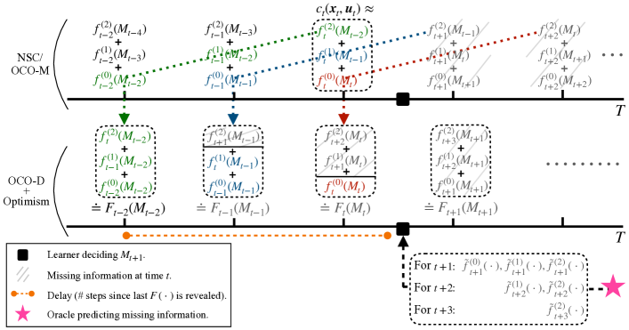
Now that we have described OptFTRL-C and characterized its policy regret, we present the main tools necessary to prove Theorem 1. Our proof is structured into two primary parts. First, we demonstrate that the regret in linearized NSC is a specific instance within the OCO-M framework, achieved through a particular selection of separable functions (sub-section IV-A, visualized in the upper timeline of Fig. 1). Second, we establish that the regret of OCO-M with separable functions is in turn a particular case within the Delayed OCO (OCO-D) framework with a specific structure of delay (sub-section IV-B, visualized in the lower timeline of Fig. 1). While the first part is fairly standard in NSC, we do not reduce its resulting OCO-M instance to standard OCO, but to OCO-D instead.
IV-A NSC with linearized costs is separable OCO-M.
In this subsection, we show how the cost at each time slot can be approximated by the sum of a finite number of functions of only the past decisions. Formally:
Lemma 1
Given , . Then for any , the following holds
Proof:
Define the counterfactual state as the state reached starting from and then executing DAC actions based on policies . In other words, this is the state reached at by following the learner’s policies but assuming that was . From (5):
| (17) |
For now, assume that . Then, by Lipschitzness:
| (18) |
However, can be written in terms of using Assumption and the definitions in (8) and (9) :
It remains to show that . From (5) and (17), we have
where follow from the sub-multipilicitive property of , and , and from . Substituting , makes the last term . ∎
The closeness of and is a known fact in NSC, and it is due to the (strong) stability assumption. Lastly, we note that it is possible to set adaptively without knowledge of by using .555This would result in a sum of the form . We leave this part for the extended version and, inline with previous works such as [15], consider here the is sufficiently large to have the approximation error as a negligible constant w.r.t. .
IV-B separable OCO-M is OCO-D
Now that we have approximated the cost at by a separable function with memory, we show in this subsection that the separated functions can be rearranged to represent an equivalent OCO with delayed feedback formulation.
Lemma 2
Let be a separable function: , . Let be an online learning algorithm whose decisions depend on the history set . Define , and the history set w.r.t. as Then,
| (19) | |||
| (20) |
(20) means that the accumulated cost, with memory, is equivalent to that of the memoryless function . However, from (19) has delayed feedback w.r.t. ; when deciding , feedback up to only is available.
Proof:
the first part is immediate from the definition of ; any with would require a function that is not in the original history set .
The second part is mainly index manipulation:
| (21) | |||
Where the first equality holds by separability, the second by shifting the sum index and using the convention , the third by using .∎
Now we are ready to prove Theorem 1:
Proof:
Denote with the cost-minimizing policy, and let be its parametrization. Then, from (2):
| (22) | ||||
| (23) |
where follows by Lemma 1, which gives both an upper bound on the learner cost and lower bound on the benchmark’s cost, by writing the sum of as a single function with memory, and by Lemma 2, with , and hence, . To bound the delayed feedback regret , we use [16, Thm. 11], which we restate below using the notation of this paper:666Mapping their notation to ours, we have , , , , , and .
Theorem 2 ([16, Thm. 11])
Now, note that the sum can be written as:
| (24) |
hence we get that
| (25) | |||
| (26) | |||
| (27) |
substituting gives the result. ∎
V Numerical Example
Recall that OptFTRL-C was designed to take advantage of a prediction oracle that forecasts future cost functions with unknown accuracy. Theorem 1 then demonstrated that the average policy regret of OptFTRL-C always converges to , but does so faster for accurate predictions. We therefore plot the policy regret of OptFTRL-C when provided with either accurate or inaccurate predictions. The implementation code of the policies OptFTRL-C, GPC, and the benchmark , as well as the code necessary to reproduce all experiments, is available at the GitHub repository [47].
We consider a system with , ,777The DAC parameter and the cost’s memory are denoted and in [1], where they are also set equal. While both are commonly referred to as “memory”, we refer to also as the delay due to the duality we presented. and hence . The dynamics are , with perturbation of maximum magnitude of . We consider a linear cost , with and hence . With these choices, we have the upper bound on the gradient .
In the accurate prediction case, we set with probability . Otherwise, we set to be uniformally random (). Hence, represents the probability of correctly predicting , and we sample it at every slot. For inaccurate prediction, we set . We compare with GPC, which was shown to outperform the classical and controllers in a wide range of situations888For additional details on the performance of GPC vs traditional ones, see the experiments in the tutorial [48], and its associated codebase [49]..
| GPC | OptFTRL-C | OptFTRL-C | Optimal | |
| Scenario (a) | ||||
| Scenario (b) | ||||
| Scenario (c) |
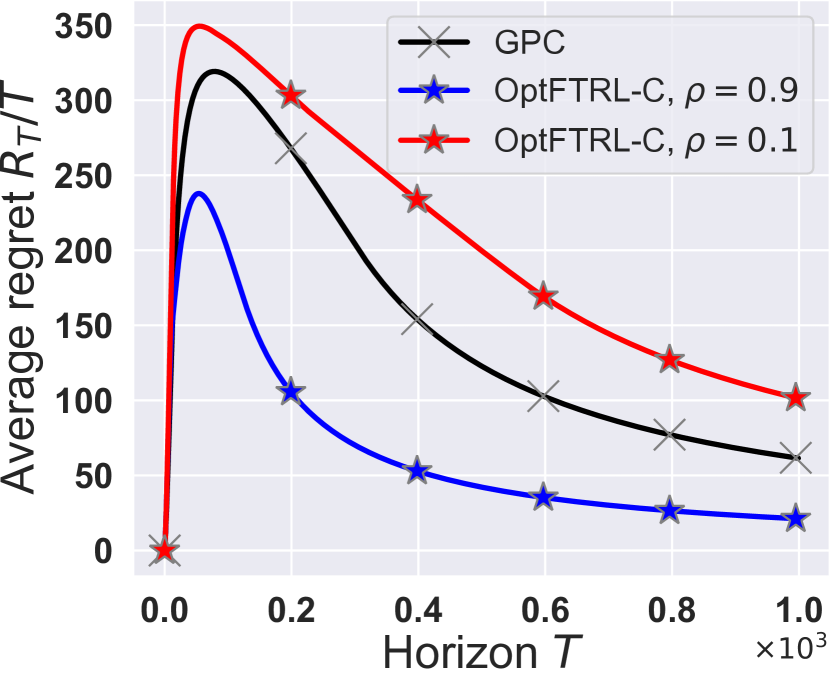
In scenario (a), The cost trajectory is set as . This represents a simple case where the cost function does not fluctuate. It can be seen from Fig. 2(a) that OptFTRL-C provides the expected acceleration when the prediction is accurate, achieving an average of smaller value compared to GPC. At the same time, the average regret still attenuates at the same rate even in the case of inaccurate predictions, but with an average performance degradation of .
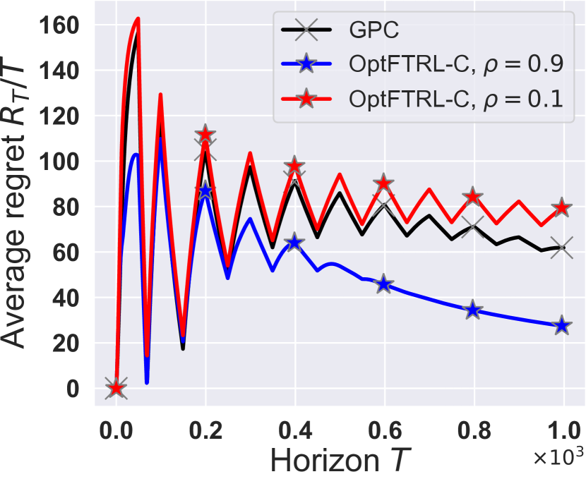
In scenario (b), we deploy an alternating cost function. Namely, alternate between and every steps. The disturbances are still . This alternating cost represents an adversarial fluctuation in the cost trajectory, and it is where the non-stochastic framework demonstrates its efficacy. Namely, this fluctuation is enough to violate the guarantees of controllers, but at the same time, it is small in magnitude, rendering controller overly pessimistic. It is worth noting that the fluctuation observed in Fig. is attributed to the update rule of GPC. This update directly modifies the decision variables based on the observed cost. In contrast, FTRL aggregates both past and future costs to determine . With accurate predictions, this method does not induce much fluctuation as it foresees the upcoming small disturbance. Overall, OptFTRL-C with good prediction achieves an improvement of in value over GPC, while having a degradation when fed with the inaccurate oracle.
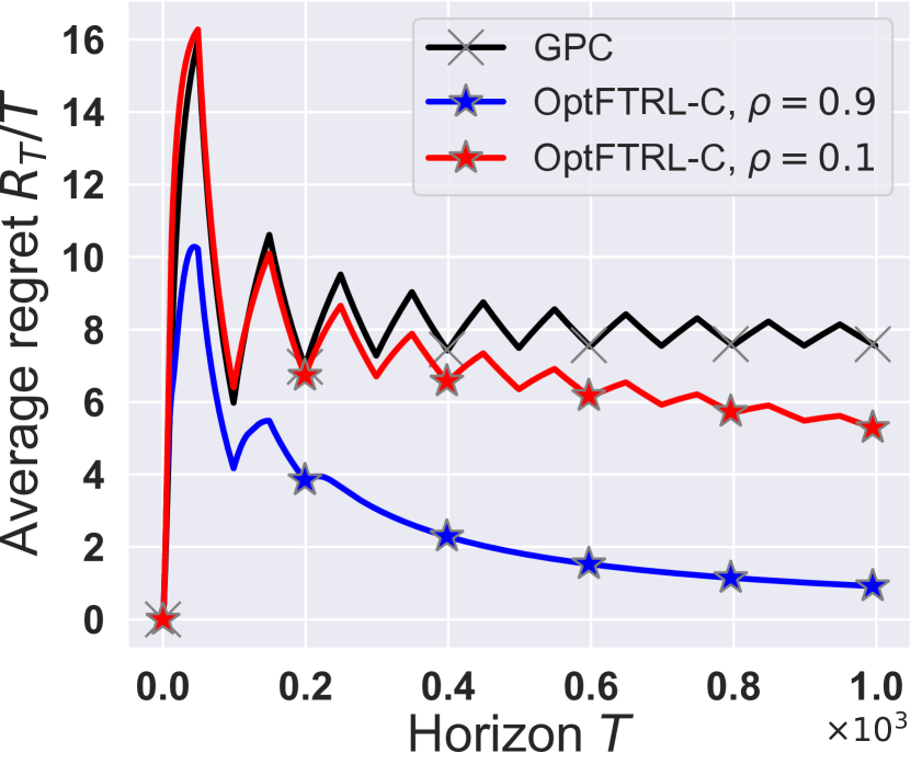
In scenario (c) we also deploy an alternating cost function but with different lower magnitudes. Namely, alternate between and every steps, and . The goal of this scenario is to show that OptFTRL-C can have an advantage over GPC even regardless of the prediction quality through adapatablity to “easy” environments (i.e., environments with small gradients). In general, GPC performance takes a hit since its learning rate is tuned with the upper bound for the gradient (i.e., ). The alternating frequency, on the other hand, contributes to distinguishing more the effect of good predictions. In this scenario OptFTRL-C achieves an improvement of and over GPC for and , respectively. In summary, OptFTRL-C leverages predictions without sacrificing its resilience to their inaccuracy, or to the costs’ adversity.
VI Conclusion
This paper looked at the NSC problem with the aim of designing DAC controllers that can leverage predictions of unknown quality. The overreaching goal is to have a controller with meaningful policy regret guarantees that are accelerated by good predictions but not void when these predictions fail. By looking at OCO-M from the lens of Delayed OCO, we were able to present the first optimistic DAC controller. Our work paves the way for further research in the ongoing pursuit of data and learning-driven control.
References
- [1] N. Agarwal, B. Bullins, E. Hazan, S. Kakade, and K. Singh, “Online control with adversarial disturbances,” in Proc. of ICML, 2019.
- [2] E. Hazan, S. Kakade, and K. Singh, “The nonstochastic control problem,” in Proc. of ALT, 2020.
- [3] A. Karapetyan, A. Iannelli, and J. Lygeros, “On the regret of h control,” in Proc. of IEEE CDC, 2022.
- [4] D. Anderson, G. Iosifidis, and D. J. Leith, “Lazy lagrangians for optimistic learning with budget constraints,” IEEE/ACM Trans. on Networking, vol. 31, no. 5, pp. 1935–1949, 2023.
- [5] N. Mhaisen, A. Sinha, G. Paschos, and G. Iosifidis, “Optimistic no-regret algorithms for discrete caching,” Proc. ACM Meas. Anal. Comput. Syst., vol. 6, no. 3, pp. 1–28, 2022.
- [6] T. Si-Salem, G. Özcan, I. Nikolaou, E. Terzi, and S. Ioannidis, “Online submodular maximization via online convex optimization,” in Proc. of AAAI, 2024.
- [7] F. Aslan, G. Iosifidis, J. A. Ayala-Romero, A. Garcia-Saavedra, and X. Costa-Perez, “Fair resource allocation in virtualized o-ran platforms,” Proc. ACM Meas. Anal. Comput. Syst., vol. 8, no. 1, 2024.
- [8] E. Hazan, “Introduction to Online Convex Optimization,” arXiv:1909.05207, 2019.
- [9] A. Rakhlin and K. Sridharan, “Online learning with predictable sequences,” in Proc. of COLT, 2013.
- [10] M. Mohri and S. Yang, “Accelerating Online Convex Optimization via Adaptive Prediction,” in Proc. of AISTATS, 2016.
- [11] O. Anava, E. Hazan, and S. Mannor, “Online learning for adversaries with memory: Price of past mistakes,” in Proc. of NeurIPS, 2015.
- [12] S. Shalev-Shwartz, “Online learning and online convex optimization,” Foundations and Trends in Machine Learning, vol. 4, no. 2, 2012.
- [13] P. Joulani, A. György, and C. Szepesvári, “A modular analysis of adaptive (non-)convex optimization: Optimism, composite objectives, and variational bounds,” in Proc. of COLT, 2017.
- [14] P. Zhao, Y.-X. Wang, and Z.-H. Zhou, “Non-stationary online learning with memory and non-stochastic control,” in Proc. of AISTATS, 2022.
- [15] H. Zhou, Z. Xu, and V. Tzoumas, “Efficient online learning with memory via frank-wolfe optimization: Algorithms with bounded dynamic regret and applications to control,” in Proc. of CDC, 2023.
- [16] G. E. Flaspohler, F. Orabona, J. Cohen, S. Mouatadid, M. Oprescu, P. Orenstein, and L. Mackey, “Online learning with optimism and delay,” in Proc. of ICML, 2021.
- [17] M. Simchowitz, “Making non-stochastic control (almost) as easy as stochastic,” in Proc. of NeurIPS, 2020.
- [18] N. Agarwal, E. Hazan, and K. Singh, “Logarithmic regret for online control,” in Proc. of NeurIPS, 2019.
- [19] D. Foster and M. Simchowitz, “Logarithmic regret for adversarial online control,” in Proc. of ICML, 2020.
- [20] Y. Li, S. Das, and N. Li, “Online optimal control with affine constraints,” in Proc. of the AAAI, 2021.
- [21] X. Liu, Z. Yang, and L. Ying, “Online nonstochastic control with adversarial and static constraints,” arXiv:2302.02426, 2023.
- [22] P. Gradu, J. Hallman, and E. Hazan, “Non-stochastic control with bandit feedback,” in Proc. of NeurIPS, 2020.
- [23] P. Gradu, E. Hazan, and E. Minasyan, “Adaptive regret for control of time-varying dynamics,” in Proc. of L4DC, 2023.
- [24] N. Mhaisen and G. Iosifidis, “Adaptive online non-stochastic control,” arXiv:2310.02261, 2023.
- [25] Z. Zhang, A. Cutkosky, and I. Paschalidis, “Adversarial tracking control via strongly adaptive online learning with memory,” in Proc. of AISTATS, 2022.
- [26] G. Shi, Y. Lin, S.-J. Chung, Y. Yue, and A. Wierman, “Online optimization with memory and competitive control,” in Proc. of NeurIPS, 2020.
- [27] G. Goel and B. Hassibi, “Competitive control,” IEEE Trans. Autom. Control, vol. 68, no. 9, pp. 5162–5173, 2023.
- [28] M. Simchowitz, K. Singh, and E. Hazan, “Improper learning for non-stochastic control,” in Proc. of COLT, 2020.
- [29] G. Goel, N. Agarwal, K. Singh, and E. Hazan, “Best of both worlds in online control: Competitive ratio and policy regret,” in Proc. of L4DC, 2023.
- [30] A. Bemporad and M. Morari, “Robust model predictive control: A survey,” in Robustness in identification and control. Springer, 2007.
- [31] G. E. Dullerud and F. Paganini, A course in robust control theory: a convex approach. Springer Science & Business Media, 2013, vol. 36.
- [32] Y. Lin, Y. Hu, G. Shi, H. Sun, G. Qu, and A. Wierman, “Perturbation-based regret analysis of predictive control in linear time varying systems,” in Proc. of NeurIPS, 2021.
- [33] Y. Lin, Y. Hu, G. Qu, T. Li, and A. Wierman, “Bounded-regret mpc via perturbation analysis: Prediction error, constraints, and nonlinearity,” in Proc. of NeurIPS, 2022.
- [34] H. B. McMahan, “A Survey of Algorithms and Analysis for Adaptive Online Learning,” J. Mach. Learn. Res., vol. 18, no. 1, 2017.
- [35] N. Mhaisen, G. Iosifidis, and D. Leith, “Online caching with no regret: Optimistic learning via recomm.” IEEE Trans. Mob. Comput., 2023.
- [36] F. Orabona, “A Modern Introduction to Online Learning,” arXiv:1912.13213, 2023.
- [37] N. Chen, A. Agarwal, A. Wierman, S. Barman, and L. L. Andrew, “Online convex optimization using predictions,” in Proc. of SIGMETRICS, 2015.
- [38] N. Chen, J. Comden, Z. Liu, A. Gandhi, and A. Wierman, “Using predictions in online optimization: Looking forward with an eye on the past,” SIGMETRICS Perform. Eval. Rev., vol. 44, no. 1, 2016.
- [39] C. Yu, G. Shi, S.-J. Chung, Y. Yue, and A. Wierman, “The power of predictions in online control,” in Proc. of NeurIPS, 2020.
- [40] Y. Li, X. Chen, and N. Li, “Online optimal control with linear dynamics and predictions: Algorithms and regret analysis,” in Proc. of NeurIPS, 2019.
- [41] R. Zhang, Y. Li, and N. Li, “On the regret analysis of online lqr control with predictions,” in Proc. of ACC, 2021.
- [42] C. Yu, G. Shi, S.-J. Chung, Y. Yue, and A. Wierman, “Competitive control with delayed imperfect information,” in Proc. of ACC, 2022.
- [43] T. Li, R. Yang, G. Qu, G. Shi, C. Yu, A. Wierman, and S. Low, “Robustness and consistency in linear quadratic control with untrusted predictions,” Proc. ACM Meas. Anal. Comput. Syst., vol. 6, no. 1, 2022.
- [44] O. Levy and Y. Mansour, “Optimism in face of a context: Regret guarantees for stochastic contextual mdp,” in Proc. of AAAI, 2023.
- [45] E. Hazan and K. Singh, “Introduction to online nonstochastic control,” arXiv:2211.09619, 2022.
- [46] A. Cohen, A. Hasidim, T. Koren, N. Lazic, Y. Mansour, and K. Talwar, “Online linear quadratic control,” in Proc. of ICML, 2018.
- [47] Optimistic-NSC. [Online]. Available: https://github.com/Naram-m/Optimistic-NSC
- [48] ICML 2021 NSC tutorial. [Online]. Available: https://icml.cc/virtual/2021/tutorial/10838
- [49] NSC-tutorial - code/experiments. [Online]. Available: https://sites.google.com/view/nsc-tutorial/codeexperiments