Gibbs measures for hardcore-SOS models on Cayley trees

Abstract.

We investigate the finite-state $p$-solid-on-solid model, for $p=\infty$, on Cayley trees of order $k\geq 2$ and establish a system of functional equations where each solution corresponds to a (splitting) Gibbs measure of the model. Our main result is that, for three states, $k=2,3$ and increasing coupling strength, the number of translation-invariant Gibbs measures behaves as $1\to 3\to 5\to 6\to 7$. This phase diagram is qualitatively similar to the one observed for three-state $p$-SOS models with $p>0$ and, in the case of $k=2$, we demonstrate that, on the level of the functional equations, the transition $p\to\infty$ is continuous.

Mathematics Subject Classifications (2022). 82B26 (primary); 60K35 (secondary)

Keywords. Cayley tree, $p$-SOS model, Gibbs measure, tree-indexed Markov chain.

1. Setting, models and functional equations

Statistical-mechanics models on trees are known to possess rich structural properties, see for example [18, 5] for general references. In the present note we contribute to this field by analyzing a hardcore model that emerges as a limit of the $p$-SOS model that was recently introduced in [3]. The setting for this $\infty$-SOS model is as follows.

Let $\Gamma^{k}=(V,L)$ be the uniform Cayley tree where each vertex has $k+1$ neighbors with $V$ being the set of vertices and $L$ the set of edges. Endpoints $x,y$ of an edge $\ell=\langle x,y\rangle$ are called nearest neighbors. On the Cayley tree there is a natural distance, to be denoted $d(x,y)$, being the smallest number of nearest-neighbors pairs in a path between the vertices $x$ and $y$, where a path is a sequence of nearest-neighbor pairs of vertices where two consecutive pairs share at least one vertex. For a fixed $x^{0}\in V$, the root, we let

$$V_{n}=\{x\in V\colon d(x,x^{0})\leq n\}\quad\text{ and }\quad W_{n}=\{x\in V\colon d(x^{0},x)=n\}$$

denote the ball of radius $n$, respectively the sphere of radius $n$, both with center at $x^{0}$. Further, let $S(x)$ be the direct successors of $x$, i.e., for $x\in W_{n}$

$$S(x)=\{y\in W_{n+1}\colon d(x,y)=1\}.$$

Next, we denote by $\Phi=\{0,1,\dots,m\}$ the local state space, i.e., the space of values of the spins associated to each vertex of the tree. Then, a configuration on the Cayley tree is a collection $\sigma=\{\sigma(x)\colon x\in V\}\in\Phi^{V}=\Omega$.

Let us now describe hardcore interactions between spins of neighboring vertices. For this, let $G=(\Phi,K)$ be a graph with vertex set $\Phi$, the set of spin values, and edge set $K$. A configuration $\sigma$ is called $G$-admissible on a Cayley tree if $\{\sigma(x),\sigma(y)\}\in K$ is an edge of $G$ for any pair of nearest neighbors $\langle x,y\rangle\in L$. We let $\Omega^{G}$ denote the sets of $G$-admissible configurations. The restriction of a configuration on a subset $A$ of $V$ is denoted by $\sigma_{A}$ and $\Omega_{A}^{G}$ denotes the set of all $G$-admissible configurations on $A$. On a general level, we further define the matrix of activity on edges of $G$ as a function

$${\lambda}\colon\{i,j\}\in K\to\lambda_{i,j}\in\mathbb{R}_{+},$$

where $\mathbb{R}_{+}$ denotes the positive real numbers and $\lambda_{i,j}$ is called the activity of the edge $\{i,j\}\in K$. In this note, we consider the graph $G$ as shown in Figure 1, which is called a hinge-graph, see for example [2].

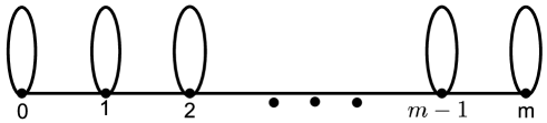
Figure 1. The hinge-graph $G$ with $m+1$ vertices.

In words, in the hinge-graph $G$, configuration are admissible only if, for any pair of nearest-neighbor vertices $\{x,y\}$, we have that

(1.1) $$|\sigma(x)-\sigma(y)|\in\{0,1\}.$$

Let us also note that our choice of admissibilities generalizes certain finite-state random homomorphism models, see [11, 6], where only configurations with $|\sigma(x)-\sigma(y)|=1$ are allowed.

Our main interest lies in the analysis of the set of splitting Gibbs measures (SGMs) defined on hinge-graph addmissible configurations. Let us start by defining SGMs for general admissibility graphs $G$. Let

$$z\colon x\mapsto z_{x}=(z_{0,x},z_{1,x},\dots,z_{m,x})\in\mathbb{R}^{m+1}_{+}$$

be a vector-valued function on $V$. Then, given $n=1,2,\ldots$ and an activity $\lambda=(\lambda_{i,j})_{\{i,j\}\in K}$, consider the probability distribution $\mu^{(n)}$ on $\Omega_{V_{n}}^{G}$, defined as

(1.2) $$\mu^{(n)}(\sigma_{n})=\frac{1}{Z_{n}}\prod_{\langle x,y\rangle\in V_{n}}\lambda_{\sigma_{n}(x),\sigma_{n}(y)}\prod_{x\in W_{n}}z_{\sigma(x),x},$$

where $\sigma_{n}=\sigma_{V_{n}}$. Here $Z_{n}$ is the partition function

$$Z_{n}=\sum_{{\widetilde{\sigma}}_{n}\in\Omega^{G}_{V_{n}}}\prod_{\langle x,y\rangle\in V_{n}}\lambda_{\widetilde{\sigma}_{n}(x),\widetilde{\sigma}_{n}(y)}\prod_{x\in W_{n}}z_{{\widetilde{\sigma}}(x),x}.$$

The sequence of probability distributions $(\mu^{(n)})_{n\geq 1}$ is called compatible if, for all $n\geq 1$ and $\sigma_{n-1}$, we have that

(1.3) $$\sum_{\omega_{n}\in\Omega^{G}_{W_{n}}}\mu^{(n)}(\sigma_{n-1}\vee\omega_{n}){\mathbf{1}}\{\sigma_{n-1}\vee\omega_{n}\in\Omega^{G}_{V_{n}}\}=\mu^{(n-1)}(\sigma_{n-1}),$$

where $\sigma_{n-1}\vee\omega_{n}$ is the concatenation of the configurations $\sigma_{n-1}$ and $\omega_{n}$. Note that, by Kolmogorov’s extension theorem, for a compatible sequence of distributions, there exists a unique measure $\mu$ on $\Omega^{G}$ such that, for all $n$ and $\sigma_{n}\in\Omega^{G}_{V_{n}}$,

$$\mu(\{\sigma|_{V_{n}}=\sigma_{n}\})=\mu^{(n)}(\sigma_{n}).$$

This motivates the following definition.

Definition 1.

We call the measure $\mu$, defined by (1.2) and (1.3), the splitting Gibbs measure corresponding to the activity $\lambda$ and the function $z\colon x\in V\setminus\{x^{0}\}\mapsto z_{x}$.

Let $A=A^{G}=\big{(}a_{ij}\big{)}_{\{i,j\}\in K}$ denote the adjacency matrix of $G$, i.e.,

$$a_{ij}=a^{G}_{ij}=\left\{\begin{array}[]{ll}1,\ \ \mbox{if}\ \ \{i,j\}\in K,\\ 0,\ \ \mbox{if}\ \ \{i,j\}\notin K,\end{array}\right.$$

then, the following statement describes conditions on $z_{x}$ guaranteeing compatibility of the distributions $(\mu^{(n)})_{n\geq 1}$.

Theorem 1.

The sequence of probability distributions $(\mu^{(n)})_{n\geq 1}$ in (1.2) are compatible if and only if, for any $x\in V$, the following system of equations holds

(1.4) $$z_{i,x}=\prod_{y\in S(x)}{\sum_{j=0}^{m-1}a_{ij}\lambda_{i,j}z_{j,y}+a_{im}\lambda_{i,m}\over\sum_{j=0}^{m-1}a_{mj}\lambda_{m,j}z_{j,y}+a_{mm}\lambda_{m,m}},\ \ i=0,1,\dots,m-1.$$

Proof.

The proof is similar to the proof of [17, Theorem 1] and [16, Proposition 2.1]. ∎

Note that, in (1.4), the normalization is at the spin state $m$, i.e., we assume that, for all $x\in V$, we have $z_{m,x}=1$.

In the remainder of the manuscript, we restrict our choice of activities in order to make contact to $p$-SOS models defined via the formal Hamiltonian

(1.5) $$H(\sigma)=-J\sum_{\langle x,y\rangle}|\sigma(x)-\sigma(y)|^{p},$$

for $p>0$ and coupling constant $J\in\mathbb{R}$, see [3, 5, 18, 19] and references therein. The present note then presents a continuation of previous investigations related to $p$-SOS models on trees with $p>0$, but now in the case where $p=\infty$. More precisely, we denote $\theta=\exp(J)$ and consider the activity $\lambda=(\lambda_{i,j})_{\{i,j\}\in K}$ defined as

(1.6) $$\lambda_{i,j}=\left\{\begin{array}[]{lll}1,\ \ \mbox{if}\ \ i=j\\[5.69054pt] \theta,\ \ \mbox{if}\ \ |i-j|=1,\\[5.69054pt] \infty,\ \ \mbox{otherwise.}\end{array}\right.$$

We call the resulting hinge-graph model (with hinge-graph as in Figure 1) the $\infty$-SOS model. Consequently, for the $\infty$-SOS model with activity (1.6), the equation (1.4) reduces to

(1.7) $$\begin{array}[]{lll}z_{0,x}=\prod_{y\in S(x)}{z_{0,y}+\theta z_{1,y}\over\theta z_{m-1,y}+1}\\[8.53581pt] z_{i,x}=\prod_{y\in S(x)}{\theta z_{i-1,y}+z_{i,y}+\theta z_{i+1,y}\over\theta z_{m-1,y}+1},\ \ i=1,\dots,m-1\\[8.53581pt] z_{m,x}=1,\end{array}$$

and, by Theorem 1, for any $z=\{z_{x}\colon x\in V\}$ satisfying (1.7), there exists a unique SGM $\mu$ for the $\infty$-SOS. However, the analysis of solutions to (1.7) for an arbitrary $m$ is challenging. We therefore restrict our attention to a smaller class of measures, namely the translation-invariant SGMs.

2. Translation-invariant SGMs for the $\infty$-SOS model with $m=2$

Searching only for translation-invariant measures, the functional equation (1.7) reduces to

(2.1) $$\begin{array}[]{lll}z_{0}=\left({z_{0}+\theta z_{1}\over\theta z_{m-1}+1}\right)^{k},\\[8.53581pt] z_{i}=\left({\theta z_{i-1}+z_{i}+\theta z_{i+1}\over\theta z_{m-1}+1}\right)^{k},\ \ i=1,\dots,m-1,\\[8.53581pt] z_{m}=1.\end{array}$$

In the following we restrict our attention to the case where $m=2$. In this case, denoting $x=\sqrt[k]{z_{0}}$ and $y=\sqrt[k]{z_{1}}$, from  (2.1) we get

(2.2) $$x={x^{k}+\theta y^{k}\over\theta y^{k}+1}\qquad\text{ and }\qquad y={\theta x^{k}+y^{k}+\theta\over\theta y^{k}+1}.$$

In particular, considering only the first equation of this system, we find the solutions $x=1$ and

(2.3) $$\theta y^{k}=x^{k-1}+x^{k-2}+\dots+x.$$

We start by investigating the case $x=1$.

2.1. Case $x=1$

In this case, from the second equation in (2.2), we get that

(2.4) $$\theta y^{k+1}-y^{k}+y-2\theta=0$$

and hence, as a direct application of Descartes’ rule of signs, the following statement follows.

Lemma 1.

For all $k\geq 2$, there exist at most three positive roots for (2.4).

For small values of $k$, i.e., $k=2,3$, we can solve (2.4) explicitly and exhibit regions of $\theta$ where there are exactly three solutions.

2.1.1. Case $k=2$

In this case, the equation (2.4) coincides with the corresponding equation for $p=\infty$ found in [7]. The solutions are presented in Section 3 below.

2.1.2. Case $k=3$

In this case, we can rearrange (2.4) as

$$\theta={y^{3}-y\over y^{4}-2}=:\alpha(y),$$

where we assumed $y\neq\sqrt[4]{2}$ since $y=\sqrt[4]{2}$ is not a solution. It follows from Figure 2 that up to three solutions $y$ for (2.4) appear as follows.

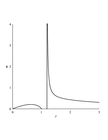
Figure 2. Graph of the function $\alpha(y)$.

There exists $\theta_{c}\approx 0.206$ such that we have:

• If $\theta\in(0,\theta_{c})$, then there are three solutions $y_{1}>\sqrt[4]{2}$ and $y_{2}<y_{3}<1$.

• If $\theta=\theta_{c}$, then there are two solutions $y_{1}>\sqrt[4]{2}$ and $y_{2}<1$.

• If $\theta>\theta_{c}$, then there is a unique solution $y_{1}>\sqrt[4]{2}$.

We can derive the value of $\theta_{c}$ explicitly as follows. The equation $\alpha^{\prime}(y)=0$ can be solved explicitly as

$$y_{0}=\sqrt{1-c+1/c}\approx 0.635,\ \ \mbox{with}\ \ c=\sqrt[3]{1+\sqrt{2}}.$$

Since $y_{0}\in(0,1)$, the critical value $\theta_{c}$ is thus given by

(2.5) $$\theta_{c}=\alpha(y_{0})={(1-c)\sqrt{c(1+c-c^{2})}\over c^{4}-3c^{2}+2c-2\sqrt{2}-1}.$$

2.2. Case $x\neq 1$

Let us consider the second situation as presented in (2.2).

2.2.1. Case $k=2$

In this case, using  (2.3) and the second equation in (2.2), we get

(2.6) $$\theta^{4}x^{4}+(2\theta^{2}-\theta)x^{3}+(2\theta^{4}-2\theta+1)x^{2}+(2\theta^{2}-\theta)x+\theta^{4}=0,$$

which is a polynomial with symmetric coefficients and hence, denoting $\xi=x+1/x$, (2.6) can be rewritten as

$$\theta^{4}(\xi^{2}-2)+(2\theta^{2}-\theta)\xi+(2\theta^{4}-2\theta+1)=0,$$

which is equivalent to

(2.7) $$\theta^{4}\xi^{2}+(2\theta^{2}-\theta)\xi+1-2\theta=0.$$

But, this equation has two solutions $\xi_{1,2}$ given in (3.7) below and thus we have up to four additional solutions. Again, this case coincides with the corresponding equation for $p=\infty$ found in [7] and the overview of solutions is presented in Section 3 below.

2.2.2. Case $k=3$

In this case, by (2.3) and the second equation in (2.2) we obtain

(2.8) $$\begin{split}\theta^{6}x^{8}+(-\theta^{6}+3\theta^{4}-\theta^{2})x^{7}+&\theta^{6}x^{6}+(2\theta^{6}-3\theta^{2}+1)x^{5}+(-2\theta^{6}+6\theta^{4}-7\theta^{2}+2)x^{4}\\ &+(2\theta^{6}-3\theta^{2}+1)x^{3}+\theta^{6}x^{2}+(-\theta^{6}+3\theta^{4}-\theta^{2})x+\theta^{6}=0\end{split}$$

and this equation may have up to eight positive solutions since, if $\theta<\theta_{c}^{\prime\prime}\approx 0.605$, the number of sign changes in the coefficients is eight. However, by computer analysis we can show that there exists $\widehat{\theta}_{c}\approx 0.4812$ such that, if $\theta<\widehat{\theta}_{c}$, then (2.8) has precisely four positive solutions, if $\theta=\widehat{\theta}_{c}$, then there are precisely two solutions and, if $\theta>\widehat{\theta}_{c}$, then there exists no positive solution (see Figure 3 for an implicit plot). For example, if $\theta=0.481$, then the four positive solutions are given approximately by

$$0.2072006567,0.2260627940,4.423549680,\text{ and }4.826239530.$$

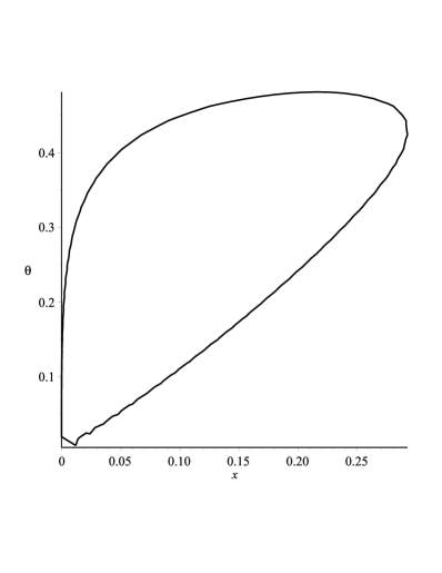
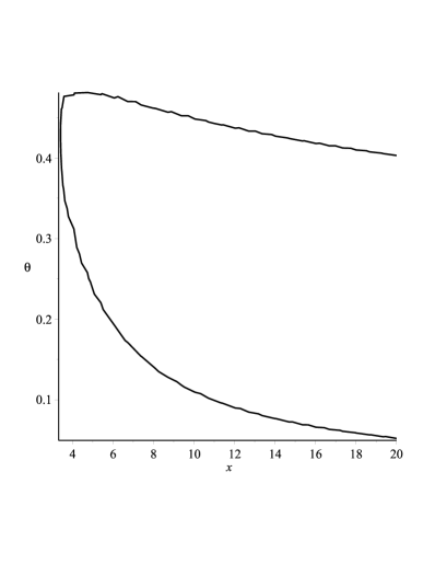
Figure 3. The implicit plot of (2.8). Left: For $\theta\in(0,\widehat{\theta}_{c})$, there are two solutions in $(0,0.2927)$. Right: For the same region of $\theta$ there are two fixed points in $(3.41,\infty)$ since both curves towards the right side converge to zero.

Let us provide an analytical proof of this as well. Since (2.8) is symmetric, we divide both sides by $x^{4}$ and denote $\eta=x+1/x$. Then, we arrive at

$$\theta^{6}((\eta^{2}-2)^{2}-2)+(-\theta^{6}+3\theta^{4}-\theta^{2})\eta(\eta^{2}-3)+\theta^{6}(\eta^{2}-2)+(2\theta^{6}-3\theta^{2}+1)\eta-2\theta^{6}+6\theta^{4}-7\theta^{2}+2=0$$

and consequently

(2.9) $$\theta^{6}\eta^{4}+(-\theta^{6}+3\theta^{4}-\theta^{2})\eta^{3}-3\theta^{6}\eta^{2}+(5\theta^{6}-9\theta^{4}+1)\eta-2\theta^{6}+6\theta^{4}-7\theta^{2}+2=0.$$

Thus, each solution $\eta>2$ of (2.9) defines two positive solutions to (2.8). Denoting $t=\theta^{2}$, we write (2.9) as the following cubic equation with respect to $t$,

$$(\eta^{4}-\eta^{3}-3\eta^{2}+5\eta-2)t^{3}+(3\eta^{3}-9\eta+6)t^{2}+(-\eta^{3}-7)t+\eta+2=0,$$

which is equivalent to

(2.10) $$(\eta-1)^{3}(\eta+2)t^{3}+3(\eta-1)^{2}(\eta+2)t^{2}-(\eta^{3}+7)t+\eta+2=0.$$

Now, again by the rule of sign changes, for each $\eta>2$, this equation may have up to two positive solution $t=\theta^{2}=t(\eta)$. For $\eta>2$ let us introduce the new variables

(2.11) $$w=(\eta-1)t>0\qquad\text{ and }\qquad E={\eta^{3}+7\over(\eta-1)(\eta+2)}=:b(\eta).$$

With this, (2.10) can be expressed as

(2.12) $$w^{3}+3w^{2}-Ew+1=0$$

and we can solve the last equation with respect to $E$, which leads to

$$E=w^{2}+3w+1/w=:a(w).$$

Note that the function $a(w)$ is monotone decreasing between $0$ and $1/2$ (because $a^{\prime}(w)=0$ has a unique positive solution $w=1/2$ and $a(0)=a(+\infty)=\infty$) and increasing when $w>1/2$. Thus, the minimal value of $E$ is given by $a(1/2)=15/4$ and hence, for each $E>15/4$, there are exactly two positive solutions $w_{1}=w_{1}(E)$ and $w_{2}=w_{2}(E)$, with $w_{1}<w_{2}$. If $E=15/4$, then there exists a unique $w_{c}=1/2$. If $E<15/4$, then there is no solution, see Figure 4.

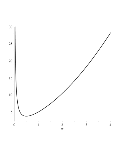
Figure 4. The graph of the function $E=a(w)$.

From Figure 4 it is also easy to see that $w_{1}(E)$ is a decreasing function with values in $(0,1/2]$ and $w_{2}(E)$ is an increasing function with values in $[1/2,\infty)$ with respect to the variable $E>15/4$. Moreover,

$$\lim_{E\to\infty}w_{1}(E)=0\qquad\text{ and }\qquad\lim_{E\to\infty}w_{2}(E)=\infty,$$

and from the function $b(\eta)$ given in (2.11), for $E=15/4$, we get that

$$\eta_{c}=(7+3\sqrt{57})/8\approx 3.707.$$

Note that, for the derivative of $\eta\mapsto b(\eta)$, we have

$$b^{\prime}(\eta)={(\eta+1)^{2}(\eta^{2}-7)\over(\eta-1)^{2}(\eta+2)^{2}}.$$

Consequently, $b(\eta)$ is increasing for $\eta>\sqrt{7}\approx 2.65$ with a minimum value $b(\sqrt{7})=21/(1+2\sqrt{7})\approx 3.34$. For each $E\geq 15/4$, since $b(\eta)$ is an increasing function, from $E=b(\eta)$ one obtains a unique $\eta\geq\eta_{c}$. As a consequence, $w_{1}(b(\eta))$ is a decreasing and $w_{2}(b(\eta))$ is an increasing functions of $\eta>\eta_{c}$. Thus, $\eta$ is a solution to the following two independent equations, obtained from the first formula of (2.11),

(2.13) $$w_{1}(b(\eta))=(\eta-1)\theta^{2}.$$

(2.14) $$w_{2}(b(\eta))=(\eta-1)\theta^{2}.$$

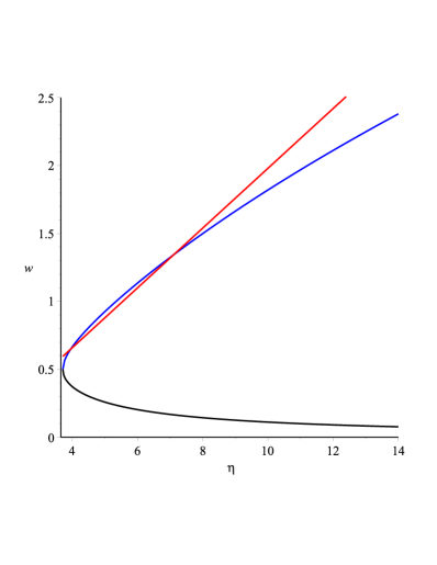
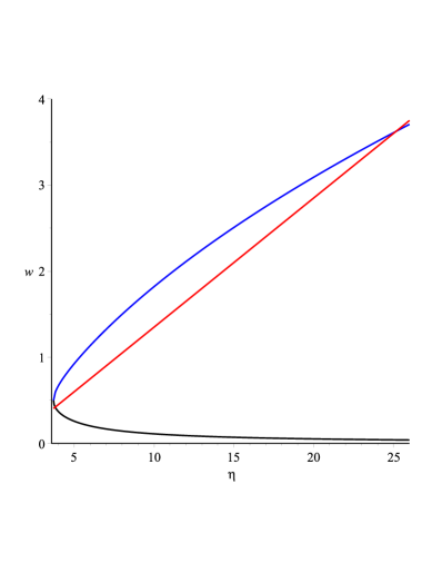
Figure 5. Up-left: The graphs of $\eta\mapsto(\eta-1)\widehat{\theta}_{c}^{2}$ (red),$\eta\mapsto w_{2}(b(\eta))$ (blue) and $\eta\mapsto w_{1}(b(\eta))$ (black). Up-right: The graphs of $\eta\mapsto(\eta-1)0.22$ (red), $\eta\mapsto w_{2}(b(\eta))$ (blue) and $\eta\mapsto w_{1}(b(\eta))$ (black). Down: The graphs of $\eta\mapsto(\eta-1)0.15$ (red), $\eta\mapsto w_{2}(b(\eta))$ (blue) and $w_{1}(b(\eta))$ (black).

Denoting by $\tilde{\theta}$ the positive solution of the equation

$$1/2=(\eta_{c}-1)\tilde{\theta}^{2},$$

see (2.11), we have

$$\tilde{\theta}={2\over\sqrt{3\sqrt{57}-1}}\approx 0.4298.$$

Then, as can be seen in Figure 5, the following assertions hold.

• If $\theta\in(0,\tilde{\theta})$, then (2.13) and (2.14) have a unique solution $\eta>2$.

• If $\theta\in[\tilde{\theta},\widehat{\theta}_{c})$, then (2.13) has no solution, but (2.14) has two solutions greater than 2.

• If $\theta=\widehat{\theta}_{c}$, then (2.13) has no solution, but (2.14) has a unique solution.

• If $\theta>\widehat{\theta}_{c}$, then both equations have no solution.

Consequently, under the above mentioned Conditions i.-ii., (2.9) has two solutions greater then 2, which define four positive solutions for (2.8).

Remark 1.

To find the exact critical value $\widehat{\theta}_{c}$ mentioned above, one has to solve the following system of equation with respect to unknowns $\widehat{\theta}_{c}$ and $\eta_{1}$

$$w_{2}^{\prime}(b(\eta_{1}))b^{\prime}(\eta_{1})=\widehat{\theta}_{c}^{2}\qquad\text{ and }\qquad w_{2}(b(\eta_{1}))=(\eta_{1}-1)\widehat{\theta}_{c}^{2}.$$

With respect to Theorem 1, we can summarize our results for $k=3$ in the following statement.

Theorem 2.

For the $\infty$-SOS model with $m=2$ and $k=3$, there exist critical values $\theta_{c}\approx 0.206$ (given explicitly by  (2.5)) and $\widehat{\theta}_{c}\approx 0.4812$ such that

• If $\theta>\widehat{\theta}_{c}$, then there is unique translation-invariant SGM.

• If $\theta=\widehat{\theta}_{c}$, then there are three translation-invariant SGMs.

• If $\theta\in(\theta_{c},\widehat{\theta}_{c})$, then there are five translation-invariant SGMs.

• If $\theta=\theta_{c}$, then there are six translation-invariant SGMs.

• If $\theta\in(0,\theta_{c})$, then there are seven translation-invariant SGMs.

3. The $p$-SOS model with $p\to\infty$

In this section we exhibit the functional equations corresponding to the $p$-SOS model defined by the Hamiltonian (1.5) and give results related to the case when $p\to\infty$. The limiting equations turn out to be the same equations as the ones for the $\infty$-SOS model. Assuming $k=m=2$, [7] establishes and analyzes the translation-invariant SGMs of the $p$-SOS model corresponding to the positive solutions of the following system

(3.1) $$x={x^{2}+\theta y^{2}+\theta^{2^{p}}\over\theta^{2^{p}}x^{2}+\theta y^{2}+1},$$

(3.2) $$y={\theta x^{2}+y^{2}+\theta\over\theta^{2^{p}}x^{2}+\theta y^{2}+1}.$$

In the following, we establish limits for the obtained solutions when $p\to\infty$. First, from (3.1) we get $x=1$ or

(3.3) $$\theta y^{2}=(1-\theta^{2^{p}})x-\theta^{2^{p}}(x^{2}+1).$$

Remark 2.

Since $x>0$ we have that (3.3) can hold iff $\theta<1$.

3.1. Case $0<\theta<1$.

Let us distinguish two subcases.

3.1.1. Case $x=1$

Solving by computer the cubic equation

(3.4) $$\theta y^{3}-y^{2}+(\theta^{2^{p}}+1)y-2\theta=0$$

and taking limits of each solution as $p\to\infty$, we see that the solutions have the limits $y_{i}(\theta)$, $i=1,2,3$. The limiting functions have lengthy formulas, but their graphs can be simply plotted as shown in Figure 7.

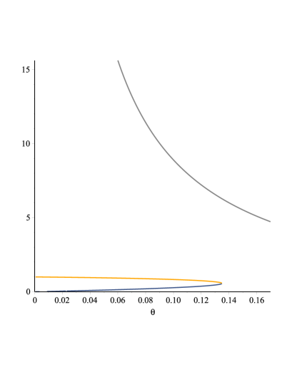
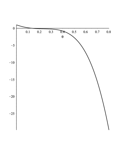
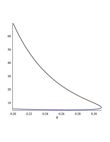
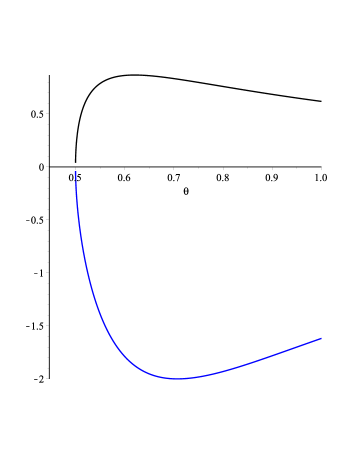
Figure 6. Left: The graphs of the functions $\theta\mapsto y_{1}(\theta)$ (gray), $\theta\mapsto y_{2}(\theta)$ (blue) and $\theta\mapsto y_{3}(\theta)$ (orange). Right: The graph of the function $\theta\mapsto\Delta_{0}(\theta)$ for $\theta\in(0,1)$.

Figure 7. Left: The graphs of the functions $\theta\mapsto\xi_{1}(\theta)$ (blue) and $\theta\mapsto\xi_{2}(\theta)$ (black) for $\theta\in(0,(\sqrt{5}-1)/4]$. Right: The same graphs for $\theta\in[{1\over 2},1)$.

Moreover, the critical value of $\theta$ for existence of more than one solution is obtained from the discriminant of the cubic equation as $p\to\infty$, i.e.,

$$\Delta_{0}(\theta)={1\over 27\theta^{2}}\left(4(1-3\theta)^{3}-(2-9\theta+54\theta^{3})^{2}\right)=0.$$

Hence, by Figure 7 it is clear that there exists a unique $\theta_{0}\approx 0.135$ such that $\Delta_{0}(\theta_{0})=0$.

3.1.2. Case $x\neq 1$

In this case, there are up to four solutions when $p>0$ is fixed. These solutions are defined by the quantities $\xi_{1}(\theta,p)<\xi_{2}(\theta,p)$ given by

(3.5) $$\xi_{1,2}(\theta,p):={q\over 2}{-3\theta q^{2}+2(\theta+1)q+2(\theta^{2}-1)\mp\theta\sqrt{q(q+2\theta-2)[(q-\theta-1)^{2}+(\theta+1)(3\theta-1)]}\over(q-\theta-1)[\theta q^{2}+(\theta^{2}-1)(q+\theta-1)]},$$

where $q=1-\theta^{2^{p}}$, see [7]. Moreover, if

(3.6) $$2<\xi_{1}(\theta,p)\leq\xi_{2}(\theta,p),$$

one can find all four positive solutions $x_{i}=x_{i}(\theta,p)$, $i=4,5,6,7$ explicitly. In this case, as $p\to\infty$, we check the Condition (3.6). From (3.5) we get

(3.7) $$\lim_{p\to\infty}\xi_{1,2}(\theta,p)=\xi_{1,2}(\theta):={1\over 2\theta^{3}}\cdot\left({1-2\theta\mp\sqrt{(2\theta-1)(4\theta^{2}+2\theta-1)}}\right)$$

and these numbers exist iff

$$(2\theta-1)(4\theta^{2}+2\theta-1)\geq 0\ \ \Leftrightarrow\ \ \theta\in(0,(\sqrt{5}-1)/4]\cup[1/2,1).$$

Thus, Condition (3.6) is satisfied iff $\theta\in(0,(\sqrt{5}-1)/4]$ (see Figure 7). Now using (3.7), for $\theta\in(0,(\sqrt{5}-1)/4))$, we obtain $x_{i}(\theta)$, $i=4,5,6,7$. Since the last $x_{i}$’s exist, we get

$$y_{i}(\theta)=\sqrt{x_{i}(\theta)/\theta},\ \ i=4,5,6,7.$$

3.2. Case $\theta>1$

In this case, assuming $x=1$, from  (3.4) we get a unique solution for large $p$, which has a limit as $p\to\infty$. If $\theta>1$ and $x\neq 1$ then the statement of Remark 2 is satisfied for any $p>0$ and therefore there is no solution. We summarize the results of this section in the following statement which essentially says that the number of translation-invariant SGMs remains unchanged in the limiting model as $p\to\infty$.

Proposition 1.

For the $p$-SOS model, as $p\to\infty$, there exist critical values $\theta_{0}\approx 0.135$ and $\theta_{0}^{\prime}=(\sqrt{5}-1)/4\approx 0.309$ such that

• If $\theta>\theta_{0}^{\prime}$, then there is a unique translation-invariant SGM.

• If $\theta=\theta_{0}^{\prime}$, then there are three translation-invariant SGMs.

• If $\theta\in(\theta_{0},\theta_{0}^{\prime})$, then there are five translation-invariant SGMs.

• If $\theta=\theta_{0}$, then there are six translation-invariant SGMs.

• If $\theta\in(0,\theta_{0})$, then there are seven translation-invariant SGMs.

4. Conditions for non-extremality of translation-invariant SGMs

It is known that a translation-invariant SGM corresponding to a vector $v=(x,y)\in\mathbb{R}^{2}$ (which is a solution to (2.2)) is a tree-indexed Markov chain with states $\{0,1,2\}$, see [5, Definition 12.2], and for the transition matrix

(4.1) $${\mathbb{P}}=\left(\begin{array}[]{ccc}{x^{k}\over x^{k}+\theta y^{k}}&{\theta y^{k}\over x^{k}+\theta y^{k}}&0\\[8.53581pt] {\theta x^{k}\over\theta x^{k}+y^{k}+\theta}&{y^{k}\over\theta x^{k}+y^{k}+\theta}&{\theta\over\theta x^{k}+y^{k}+\theta}\\[8.53581pt] 0&{\theta y^{k}\over\theta y^{k}+1}&{1\over\theta y^{k}+1}\end{array}\right).$$

Hence, for each given solution $(x_{i},y_{i})$, $i=1,\dots,7$ of (2.2), we need to calculate the eigenvalues of $\mathbb{P}$. The first eigenvalue is one since we deal with a stochastic matrix, the other two eigenvalues

(4.2) $$\lambda_{j}(x_{i},y_{i},\theta,k),\qquad j=1,2,$$

can be found via symbolic computer analysis, but they have bulky formulas. For example, in the case $x=1$, for each $y$ the matrix (4.1) has three eigenvalues, 1 and

$$\lambda_{1}(1,y,\theta,k)={(1-2\theta^{2})y^{k}\over\theta y^{2k}+(2\theta^{2}+1)y^{k}+2\theta}\qquad\text{and}\qquad\lambda_{2}(1,y,\theta,k)={1\over\theta y^{k}+1}.$$

However, we can still deduce the following relation.

Lemma 2.

If $\theta\in(0,1)$, then, for any solution $y$ of (2.4), we have that

$$|\lambda_{1}(1,y,\theta,k)|\leq\lambda_{2}(1,y,\theta,k).$$

Proof.

Since $\lambda_{2}>0$, we have to show that

(4.3) $$-\lambda_{2}(1,y,\theta,k)\leq\lambda_{1}(1,y,\theta,k)\leq\lambda_{2}(1,y,\theta,k).$$

It is easy to see that the inequality on the left is true for $\theta$ satisfying $1-2\theta^{2}\geq 0$. If $1-2\theta^{2}<0$ then the inequality on the left is equivalent to

$$\theta(1-\theta^{2})y^{2k}+y^{k}+\theta\geq 0,$$

which is true for all $\theta<1$. Next, the inequality on the right of (4.3) is equivalent to the inequality

$$(\theta y^{k}+1)^{2}\geq 0,$$

which is universally true, concluding the proof. ∎

Now, a sufficient condition for non-extremality of a Gibbs measure $\mu$ corresponding to ${\mathbb{P}}$ on a Cayley tree of order $k\geq 1$ is given by the Kesten–Stigum Condition $k\lambda^{2}>1$, where $\lambda$ is the second-largest (in absolute value) eigenvalue of ${\mathbb{P}}$, see [8]. Hence, denoting for $i=1,\dots,7$,

$$\eta_{i}(\theta,k)=k\lambda^{2}_{2}(x_{i},y_{i},\theta,k)-1\qquad\text{ and }\qquad\mathbb{K}_{i}=\{(\theta,k)\in(0,1)\times\mathbb{N}\colon\eta_{i}(\theta,k)>0\},$$

using Lemma 2, we have the following criterion.

Proposition 2.

Let $\mu_{i}$ denote the translation-invariant SGM associated to the tuple $(x_{i},y_{i},\theta,k)$. If $(\theta,k)\in\mathbb{K}_{i}$ then $\mu_{i}$ is non-extremal.

In order to employ the proposition, for $k=2$ and $k=3$, we find representations for $\mathbb{K}_{i}$. In case $k=2$ and $x_{i}=1$, we have for $i=1,2,3$ that $\lambda_{2}(1,y_{i},\theta,2)=1/(\theta y_{i}^{2}+1)$ and thus

$$\eta_{i}(\theta,2)={2\over(\theta y_{i}^{2}+1)^{2}}-1.$$

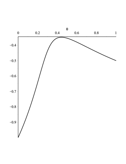
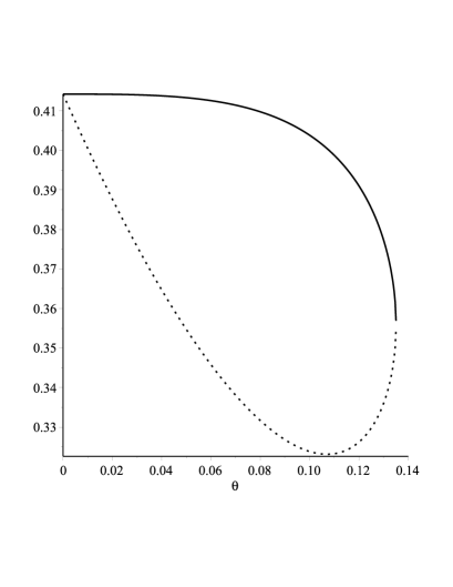
Figure 8. Left: The graph of the function $\eta_{1}(\theta,2)$, $\theta\in(0,1)$. Right: The graphs of the functions $\eta_{2}(\theta,2)$ (solid line) and $\eta_{3}(\theta,2)$ (doted line) when $\theta\in(0,0.14)$.

Hence, from Figure 8 it follows that, for $\mu_{1}$, the Kesten–Stigum condition is never satisfied, but for $\mu_{2}$ and $\mu_{3}$ the condition is always satisfied, i.e., $\mu_{2}$ and $\mu_{3}$ are not-extreme.

In case $k=3$ and $x_{i}=1$, we have for $i=1,2,3$, using $\lambda_{2}(1,y_{i},\theta,3)=1/(\theta y_{i}^{3}+1)$, that

$$\eta_{i}(\theta,3)={3\over(\theta y_{i}^{3}+1)^{2}}-1.$$

But, as shown in Section 2.1.2, if $\theta<\theta_{c}\approx 0.206$, there exist two solutions $y_{2},y_{3}<1$. For these solutions we have

$$\eta_{i}(\theta,3)={3\over(\theta y_{i}^{3}+1)^{2}}-1>{3\over(\theta+1)^{2}}-1.$$

But, since $\theta<\theta_{c}$, we have that $3/(\theta+1)^{2}-1>0$ and we can formulate the following summarizing result.

Proposition 3.

For $\theta<1$, $k=2$ and $k=3$ the translation-invariant SGMs corresponding to solutions of the form $(1,y)$ with $y<1$ are not-extreme.

Let us note that for $k=3$ and $x_{i}=1$ the translation-invariant SGM corresponding to the solution $y_{1}>\sqrt[4]{2}$ does not satisfy the Kesten–Stigum condition if $\theta>(\sqrt{3}-1)/\sqrt[4]{8}\approx 0.435.$ Indeed, using $y_{1}>\sqrt[4]{2}$ we get

$$\eta_{i}(\theta,3)={3\over(\theta y_{1}^{3}+1)^{2}}-1<{3\over(\theta\sqrt[4]{8}+1)^{2}}-1<0\ \ \Leftrightarrow\ \ \theta>{\sqrt{3}-1\over\sqrt[4]{8}}.$$

Remark 3.

Let us finally discuss further extremality conditions for translation-invariant SGMs. Various approaches in the literature aim to establish sufficient conditions for extremality, which can be simplified to a finite-dimensional optimization problem based solely on the transition matrix. For instance, the percolation method proposed in [13] and [14], the symmetric-entropy method by [4], or the bound provided in [12] for the Ising model in the presence of an external field. Different techniques are employed also in [1] in order to demonstrate the sharpness of the Kesten-Stigum bound for an Ising channel with minimal asymmetry.

However, since, in our case, the transition matrix corresponding to a translation-invariant SGM depends on the solutions $(x_{i},y_{i})$, which have a very complex form, it appears challenging to apply the aforementioned methods to verify extremality. Furthermore, the difficulty increases when we only have knowledge of the existence of a solution but lack its explicit form. Nonetheless, our results could serve as a basis for numerical investigations of extremality in the future.

References

- [1] C. Borgs, J. Chayes, E. Mossel, S. Roch, The Kesten-Stigum reconstruction bound is tight for roughly symmetric binary channels, FOCS, 2006, 47th Annual IEEE Conference on Foundations of Computer Science, 518–530. Preprint arXiv:math/0604366v1.
- [2] G.R. Brightwell, P. Winkler, Graph homomorphisms and phase transitions, J. Combin. Theory Ser. B 77(2) (1999), 221–262.
- [3] L. Coquille, C. Külske, A. Le Ny, Extremal inhomogeneous Gibbs states for SOS-models and finite-spin models on trees, J. Stat. Phys. 190 (2023), 71–97.
- [4] M. Formentin, C. Külske, A symmetric entropy bound on the non-reconstruction regime of Markov chains on Galton-Watson trees. Electron. Commun. Probab. 14 (2009), 587–596.
- [5] H.-O. Georgii, Gibbs Measures and Phase Transitions, Second edition. de Gruyter Studies in Mathematics, 9. Walter de Gruyter, Berlin, 2011.
- [6] B. Jahnel, C. Külske, U.A. Rozikov, Gradient Gibbs measures for the random homomorphism model on Cayley trees. In preparation.
- [7] B. Jahnel, U.A. Rozikov, Three-state p-SOS models on binary Cayley trees. arXiv:2402.09839
- [8] H. Kesten, B.P. Stigum, Additional limit theorem for indecomposable multi-dimensional Galton–Watson processes, Ann. Math. Statist. 37 (1966), 1463–1481.
- [9] C. Külske, U.A. Rozikov, Extremality of translation-invariant phases for a three-state SOS-model on the binary tree, J. Stat. Phys. 160(3) (2015), 659–680.
- [10] C. Külske, U.A. Rozikov, Fuzzy transformations and extremality of Gibbs measures for the Potts model on a Cayley tree, Random Struct. Algorithms. 50(4) (2017), 636–678.
- [11] P. Lammers, F. Toninelli: Height function localisation on trees, Comb. Probab, 33(1) (2024), 50–64.
- [12] J.B. Martin, Reconstruction thresholds on regular trees. Discrete random walks (Paris, 2003), 191–204 (electronic), Discrete Math. Theor. Comput. Sci. Proc., AC, Assoc. Discrete Math. Theor. Comput. Sci., Nancy, 2003.
- [13] F. Martinelli, A. Sinclair, D. Weitz, Fast mixing for independent sets, coloring and other models on trees, Random Struct. Algorithms, 31 (2007), 134–172.
- [14] E. Mossel, Y. Peres, Information flow on trees, Ann. Appl. Probab. 13(3) (2003), 817–844.
- [15] E. Mossel, Survey: Information flow on trees, Graphs, Morphisms and Statistical Physics, 155–170, DIMACS Ser. Discrete Math. Theoret. Comput. Sci., 63, Amer. Math. Soc., Providence, RI, 2004.
- [16] U.A. Rozikov, Y.M. Suhov, Gibbs measures for SOS model on a Cayley tree, Infin. Dimens. Anal. Quantum Probab. Relat. Top. 9(3) (2006), 471–488.
- [17] U.A. Rozikov, Sh.A. Shoyusupov, Fertile three state HC models on Cayley tree, Theor. Math. Phys. 156(3) (2008), 1319–1330.
- [18] U.A. Rozikov, Gibbs Measures on Cayley Trees, World Sci. Publ. Singapore. 2013.
- [19] U.A. Rozikov, Gibbs Measures in Biology and Physics: The Potts model, World Sci. Publ. Singapore. 2022.