The power of a single Haar random state: constructing and separating quantum pseudorandomness

Boyang Chenโ€‰ Institute for Interdisciplinary Information Sciences, Tsinghua University 0009-0000-1043-0977 Andrea Coladangelo Paul G. Allen School of Computer Science & Engineering, University of Washington Or Sattath Computer Science Department, Ben-Gurion University of the Negev
Abstract

In this work, we focus on the following question: what are the cryptographic implications of having access to an oracle that provides a single Haar random quantum state? We show, perhaps surprisingly, that such an oracle is sufficient to construct quantum pseudorandomness.

Pseudorandom states (PRS) are a family of states for which it is hard to distinguish between polynomially many copies of either a state sampled uniformly from the family or a Haar random state. A weaker notion, called single-copy pseudorandom states (${\mathsf{1PRS}}$), satisfies this property with respect to a single copy. Our main result is that ${\mathsf{1PRS}}$ (as well as bit-commitments) exist relative to an oracle that provides a single Haar random state. We build on this result to show the existence of an oracle relative to which ${\mathsf{1PRS}}$ exist, but ${\mathsf{PRS}}$ do not. This provides one of the first black-box separations between different forms of quantum pseudorandomness.

1 Introduction

It is well known that computational assumptions are necessary for almost all modern classical and quantum cryptographic tasks. The minimal assumption that is useful for classical cryptography is the existence of one-way functions (${\mathsf{OWF}}$). This assumption is known to be equivalent to the existence of many other cryptographic applications, such as pseudorandom number generators, pseudorandom functions, digital signatures, symmetric-key encryption, and commitments (see, e.g.,ย [Gol01, Gol04]).

The quantum setting presents a drastically different picture: a variety of quantum primitives are known that are sufficient to build cryptography, but are potentially weaker than one-way functions. Recently, Tomoyuki Morimae coined the term MicroCrypt, as an addition to Impagliazzoโ€™s five worldsย [Imp95], to refer to such quantum primitives (and their cryptographic applications)111As far as we know, Morimae introduced the term in a talk https://www.youtube.com/live/PKfYJlKD3z8?feature=share&t=1048, though he did not provide a precise definition, so our definition might be slightly different than his original intention.. One of the tenants of MicroCrypt are pseudorandom states (๐–ฏ๐–ฑ๐–ฒ๐–ฏ๐–ฑ๐–ฒ{\mathsf{PRS}}), first introduced by Ji, Liu, and Songย [JLS18]. This is a family of efficiently generatable quantum states {|ฯ•kโŸฉ}kโˆˆ{0,1}nsubscriptketsubscriptitalic-ฯ•๐‘˜๐‘˜superscript01๐‘›\{\ket{\phi_{k}}\}_{k\in\{0,1\}^{n}} such that it is computationally hard to distinguish between polynomially many copies of (a) |ฯ•kโŸฉketsubscriptitalic-ฯ•๐‘˜\ket{\phi_{k}} sampled uniformly from the family, and (b) a uniformly (Haar) random quantum state. Ji, Liu, and Song also provided a black-box construction of ๐–ฏ๐–ฑ๐–ฒ๐–ฏ๐–ฑ๐–ฒ{\mathsf{PRS}} from a ๐–ฎ๐–ถ๐–ฅ๐–ฎ๐–ถ๐–ฅ{\mathsf{OWF}}. Subsequent to [JLS18], many other tenants of MicroCrypt have been introduced, such as pseudorandom function-like states (๐–ฏ๐–ฑ๐–ฅ๐–ฒ๐–ฏ๐–ฑ๐–ฅ๐–ฒ{\mathsf{PRFS}})ย [AGQY22], efficiently samplable statistically far-but-computationally-indistinguishable pairs of (mixed) quantum states (๐–ค๐–ฅ๐–จ๐–ค๐–ฅ๐–จ{\mathsf{EFI}} pairs)ย [Yan22, BCQ23], one-way state generatorsย [MY22b], and pseudorandom states with proof of destructionย [BBSS23].

Many cryptographic applications are known based on MicroCrypt assumptions. By now, variants of all of the main MiniCrypt222Minicrypt primitives are those that are equivalent to one-way functions. The term was introduced by Impagliazzo [Imp95]. primitives have been shown to be in MicroCrypt, including symmetric-key encryption, commitments (recently, also commitments to quantum statesย [GJMZ23]), PRGs, PRFs, garbled circuits, message authentication codes, and digital signatures. Perhaps more surprisingly, MicroCrypt also contains some tasks in Cryptomania, namely, secure multi-party computationย [MY22b, BCKM21, GLSV21] and public-key encryption with quantum public keysย [BGHD+23]. The key factor contributing to the surprise is Impagliazzo and Rudichโ€™s separation between one-way functions (MiniCrypt) and public-key encryption333Note that this classical separation does not apply for public key encryption with quantum public keys. and oblivious transfer (Cryptomania)ย [IR89]. The new constructions circumvent classical impossibilities because they involve quantum states, e.g.ย commitments and multiparty computation rely on quantum communication, and encryption schemes have quantum ciphertexts.

The evidence that these quantum primitives are weaker than MiniCrypt comes from Kretschmerโ€™s quantum oracle separation of ${\mathsf{PRS}}$ and ${\mathsf{OWF}}$s [Kre21]. The separating oracle consists of a family $\{\mathcal{U}_{n}\}_{n\in\mathbb{N}}$, where $\mathcal{U}_{n}$ is a list of exponentially many Haar random $n$-qubit unitaries $\{U_{k}\}_{k\in\{0,1\}^{n}}$. Relative to this oracle, there is a simple construction of a ${\mathsf{PRS}}$: for $k\in\{0,1\}^{n}$, let $\ket{\phi_{k}}:=U_{k}\ket{0^{n}}$. Note that, if we just consider the action of the unitaries $U_{k}$ on the standard basis states, i.e.ย the set of states $U_{k}\ket{x}$ for $x\in\{0,1\}^{n}$, then, for each $n$, Kretschmerโ€™s oracle can be viewed as providing $2^{2n}$ โ€œessentially Haar randomโ€ states444The states are Haar random subject to the constraint that they should be pairwise orthogonal (for each fixed $k$).. In another work, Bouland, Fefferman and Vaziraniย [BFV19] show555Modulo a technical gap in their proofย [BFV19, p.ย 19]: โ€We expect the same result would apply โ€ฆbut we do not prove this fact.โ€ a ${\mathsf{PRS}}$ construction relative to a family $\{\mathcal{U}_{n}\}_{n\in\mathbb{N}}$, where $\mathcal{U}_{n}=(U,U^{-1})$ for a Haar random $n$-qubit $U$. By considering the action of $U$ on the standard basis states, this oracle can be viewed as providing $2^{n}$ essentially Haar random states. This raises a natural question. What can be done with much fewer Haar random states? We look at the most extreme case and ask:

What are the cryptographic implications of having oracle access to a single Haar random state?666Or, more precisely, one $n$-qubit Haar random state for each value of $n$ (which is accessed by providing the input $1^{n}$).

We define the common Haar random stateย (CHRS) model, where all the parties (including the adversary) have access to an arbitrary polynomial number of copies of a single Haar random state. Is quantum pseudorandomness possible in this model? In the classical setting, having access to a fixed (random) string, which can be used both by the algorithm and the adversary, is not enough to construct pseudorandomness (e.g., pseudorandom generators). In the quantum setting, one may naturally expect that, similarly, a single Haar random state is not enough to construct quantum pseudorandomness.

The ${\mathsf{PRS}}$ variant that is most relevant for this work is single-copy pseudorandom states (${\mathsf{1PRS}}$), introduced by Morimae and Yamakawaย [MY22a]. They differ from (multi-copy) pseudorandom states (${\mathsf{PRS}}$) in two important ways (see Definitionย 3.2 for a formal definition):

  1. 1.

    The adversary needs to distinguish between a single copy of the pseudorandom state and a single copy of a Haar random state.

  2. 2.

    The construction has to be โ€œstretchingโ€: the number of output qubits has to be greater than the key size (for this to be a non-trivial object).

1.1 Our results

Our first result is that, perhaps surprisingly, single-copy pseudorandom states exist in this model:

Theorem 1.1 (Informal).

${\mathsf{1PRS}}$ exist in the CHRSย model.

The ${\mathsf{1PRS}}$ is statistically secure as long as the number of copies of the Haar random state that the adversary receives is polynomial. This result is shown in Sectionย 4. One of the main technical ingredients that we introduce to prove Theoremย 1.1 is a certain โ€œstretchingโ€ result for quantum pseudorandomness in the CHRS model (Theoremย 2.2 in the technical overview, and Theoremย 4.6 in the main text), which may find application elsewhere.

As a result, we show that the statistical ${\mathsf{1PRS}}$ above can be used to achieve a surprisingly strong form of bit-commitment:

Theorem 1.2 (Informal).

In the CHRSย model, a non-interactive quantum bit-commitment exists that is statistically hiding and binding.

The hiding property holds against a computationally unbounded adversary that receives any polynomial number of copies of the Haar random state. In contrast, the binding property holds against a computationally unbounded adversary with an unbounded number of copies. Such statistical binding and hiding cannot exist in the standard modelย [LC97, May97]. The theorem above is proven in Appendixย A, in a similar way as shown previously by [MNY23]. Thanks to Theorem 14 in [Qia23], the commitment scheme that we obtain in the CHRS model can be compiled into an $\epsilon$-simulation secure one, using an adaption of the compiler from [BCKM21]. This version of commitment is sufficient to build secure multiparty computation via the construction in [BCKM21].

Even though plenty of relations involving MicroCrypt primitives are known, the only black-box separations involving MicroCrypt are the following: Kretschmerย [Kre21] separated post-quantum ${\mathsf{OWF}}$ from ${\mathsf{PRS}}$, via a quantum oracle. Ananth, Qian and Yuenย [AQY22] observed that this separation also separates ${\mathsf{OWF}}$ from ${\mathsf{PRFS}}$. Kretschmer et al.ย [KQST23] separated ${\mathsf{OWF}}$ from ${\mathsf{1PRS}}$ via a classical oracle. However, when we zoom in on MicroCrypt, almost nothing is known about whether different MicroCrypt primitives are equivalent to each other, or whether there is a hierarchy. The only known non-trivial [BS20] (see also [ALY23, p.3]) that PRS with very short output ($c\cdot\log(n)$ for $c\ll 1$, where $n$ is the length of the key) exist unconditionally. Hence, they are trivially black-box separated from all of the other MicroCrypt primitives which require computational assumptions. separation is between short output and long output ${\mathsf{PRS}}$ (with the former being potentially stronger). This separation is an immediate consequence of the works of Barhoush et al. [BBO+24] (which gives a construction of quantum digital signatures from PRS with short output) and Coladangelo and Mutreja [CM24] (which shows an oracle separation between quantum digital signatures and PRS with long output), and was also shown in a concurrent work of Bouazizโ€“Ermann and Muguruza [BEM24].

In this work, building on our Theoremย 1.1, we show a second black-box separation within MicroCrypt:

Theorem 1.3 (Informal).

There is a quantum oracle relative to which ${\mathsf{1PRS}}$ exist, but ${\mathsf{PRS}}$ (with output length at least $\log n+10$, where $n$ is the seed length) do not.777This quantum oracle consists of an isometry that provides a fixed Haar random state, along with a QPSPACE machine. While the latter is a unitary oracle, the former is not. In Section 5.3, we formally discuss various notions of black-box oracle separations and their implications in terms of the impossibility of black-box constructions. In particular, Theorem 1.3 implies that there cannot be a fully black-box construction of a ${\mathsf{PRS}}$ from a ${\mathsf{1PRS}}$ that uses the ${\mathsf{1PRS}}$ as an isometry (see Section 5.3 for more details).

The separation is essentially tight in terms of output length, since PRS with very short output ($c\cdot\log(n)$ for $c\ll 1$) exist unconditionally [BS20]. We show this result in Sectionย 5. Of course, this indicates that relative to the same oracle, primitives which imply a black-box construction of ${\mathsf{PRS}}$, such as ${\mathsf{OWF}}$ (as shown inย [JLS18]) and ${\mathsf{PRFS}}$, also cannot exist.

Related work.

In this work, we introduce the common Haar random stateย (CHRS) model, in which both the generation algorithm and the adversary have access to polynomially many copies of a Haar random state over $n$ qubits. There are two related models. The first, which our work is a particular case of, was called the quantum auxiliary input model (where the quantum state is sometimes referred to as the quantum advice) byย [MNY23], in which the parties are provided with polynomially many copies of a quantum state, which need not be efficiently generatable888We prefer not to use the term โ€œquantum auxiliary inputโ€ since in most other works we are aware of (seeย [DGK+10] and references therein), a quantum auxiliary input typically represents a setting in which the adversary may have information that may depend on the honest partiesโ€™ inputs, and in particular, the secret key. In contrast, in our setting and that of [MNY23], the โ€œauxiliaryโ€ state is fixed, independently of any honest partiesโ€™ input.. Chailloux, Kerenidis, and Rosgenย [CKR16] showed that quantum commitments with quantum auxiliary input exist under a computational assumption. They provide two schemes, where either the hiding or binding properties are computational. Morimae, Nehoran, and Yamakawaย [MNY23] and Qianย [Qia23] recently proved, unconditionally, the existence of a computationally hiding and statistically binding commitment in the quantum auxiliary input model. This improves on the result ofย [CKR16], in the sense that the computational assumption is removed.

The second related model is the common reference quantum state (CRQS) model, in which the quantum state needs to be efficiently generatable. Note that, in the classical setting, the common reference string represents a model with a trusted setup. In this model, [MNY23], show a statistically hiding and binding commitment with similar properties to ours. The difference is in the order of quantifiers of the hiding property: in our work, the scheme is hiding against an adversary that is allowed to have any polynomial number of copies of the quantum (Haar-random) state; in their construction (seeย [MNY23, Theorem 1.4]), they first pick a polynomial $t(n)$ and show a construction which is hiding against adversaries which receive $t(n)$ copies of the CRQS999Even though this was not formally claimed inย [MNY23], we believe that the construction mentioned in the previous paragraph, with (inefficiently generatable) auxiliary quantum inputs, satisfies the same statistical security guarantees as ours.. Of course, the main disadvantage of our work is that a Haar random state cannot be efficiently generated, whereas the state they use is efficiently generatable. However, note that if one is satisfied with security against some fixed polynomial $t(n)$ of copies, the Haar random state can be replaced efficiently by a quantum $t(n)$-design.

We emphasize the features that differentiate our work:

  • (i)

    Our common random state is structure-less: it is a Haar random state.

  • (ii)

    We show how to achieve quantum pseudorandomness in this model. The related works construct commitments directly, but their constructions do not have any implications with regard to quantum pseudorandomness. We find it quite surprising that a Haar random state alone can yield quantum pseudorandomness. It is also thanks to this connection that we are able to separate different flavors of quantum pseudorandomness, namely ${\mathsf{1PRS}}$ and ${\mathsf{PRS}}$.

Recently, many results regarding MicroCrypt have been discoveredโ€”at this point, too many to cover in detail. A diagram showing the different MicroCrypt primitives, their relations, applications, and separations are depicted in Fig.ย 3 on Fig.ย 3.

Open problems.

This work opens up several directions for further research.

  • โ€ข

    Our separation result (Theoremย 1.3) holds relative to a quantum oracle. Can it be shown relative to a classical oracle? We note that Krethschmer et al.ย [KQST23] show a classical oracle relative to which ${\mathsf{1PRS}}$ and commitments exist, but one-way functions do not.

  • โ€ข

    As pointed out earlier, since our separating oracle is technically an isometry, Theoremย 1.3 implies that there does not exist a fully black-box construction of a ${\mathsf{PRS}}$ from a ${\mathsf{1PRS}}$ that uses the ${\mathsf{1PRS}}$ as an isometry (see Sectionย 5.3 for more details). An open question is to rule out the most general kind of black-box construction, which can make use of a unitary implementation of the ${\mathsf{1PRS}}$ (as well as its inverse).

  • โ€ข

    There are examples of primitives that we know can be constructed from ${\mathsf{PRS}}$, but are not known to be implied by ${\mathsf{1PRS}}$. The main examples are one-time digital signatures with quantum public keysย [MY22a], private quantum coinsย [JLS18], and quantum pseudo-encryptionย [AQY22]. Currently, we do not have a separation between those applications101010or even ones which are based on stronger MicroCrypt assumptions, such as the existence of long input ${\mathsf{PRFS}}$, which can be used to construct message authentication codes with quantum tagsย [AQY22], quantum symmetric key encryptionย [AQY22], and public key encryption with quantum ciphers and quantum public keysย [BGHD+23]. and ${\mathsf{1PRS}}$. Understanding whether any of these applications are separated from ${\mathsf{1PRS}}$ would be interesting.

  • โ€ข

    Lastly, in the plain model, โ€œflavor conversionโ€ย [Yan22, HMY23] allows switching between the computational and statistical hiding and binding properties. In our work, the commitment is statistically hiding against adversaries with polynomially many copies of the Haar random state. It is statistically binding against adversaries with an arbitrary number of copies of the Haar random state. Is there a flavor conversion theoremโ€”this time, regarding the number of copies of the state that the adversary holdsโ€”that holds in our setting?

Acknowledgments

AC and OS thank NTT research and Mark Zhandry for organizing the quantum money workshop, as well as the participants of the workshop, where this research was initiated. BC thanks Xingjian Li for helpful discussions.

[Uncaptioned image]

OS was funded by the European Union (ERC-2022-COG, ACQUA, 101087742). Views and opinions expressed are however those of the author(s) only and do not necessarily reflect those of the European Union or the European Research Council Executive Agency. Neither the European Union nor the granting authority can be held responsible for them.

2 Technical Overview

This section is organized as follows. In Sectionย 2.1, we describe the construction of a ${\mathsf{1PRS}}$ in the CHRSย model, and we give a high-level overview of the proof of security. We view this as the main technical contribution of our work. In Sectionย 2.2, we explain how to construct statistically binding commitments from the constructed ${\mathsf{1PRS}}$ (this follows the approach of [MNY23]). Finally, in Sectionย 2.3, we describe an oracle separation between ${\mathsf{1PRS}}$ and ${\mathsf{PRS}}$. We consider the CHRS model augmented with quantum oracle access to a QPSPACE machine, and we describe a generic attack on any ${\mathsf{PRS}}$ construction in this model. Since ${\mathsf{1PRS}}$ still exist in this model, this yields an oracle separation between the two.

2.1 Construction of ${\mathsf{1PRS}}$ in the CHRSย model

${\mathsf{1PRS}}$ definition.

Recall that, informally, a ${\mathsf{1PRS}}$ is a QPT algorithm that takes as input a seed $k\in\{0,1\}^{n}$ (where $n$ is a security parameter) and outputs a state of some length $m>n$. We denote by $\ket{\phi_{k}}$ the output state on seed $k$. Then, security requires that a single copy of the ${\mathsf{1PRS}}$ state be computationally indistinguishable from a single maximally mixed state of the same dimension, i.e.

$$\mathbb{E}_{k}\,\ket{\phi_{k}}\bra{\phi_{k}}\approx_{c}\frac{\mathds{1}}{2^{m}}$$

(where $\approx_{c}$ denotes computational indistinguishability).

Note that this requirement is only non-trivial when $m>n$ (otherwise, one can simply output the seed itself). Equivalently, one can think of the problem of constructing a ${\mathsf{1PRS}}$ as the problem of finding a family $\{U_{k}\}_{k\in\{0,1\}^{n}}$ of efficiently computable unitaries such that

๐”ผkโ€‹Ukโ€‹|0โŸฉโ€‹โŸจ0|โ€‹Ukโ€ โ‰ˆc๐Ÿ™2m.subscript๐‘subscript๐”ผ๐‘˜subscript๐‘ˆ๐‘˜ket0bra0superscriptsubscript๐‘ˆ๐‘˜โ€ 1superscript2๐‘š\mathbb{E}_{k}\,U_{k}\ket{0}\bra{0}U_{k}^{\dagger}\approx_{c}\frac{\mathds{1}}{2^{m}}\,.

This problem becomes trivial if the family $\{U_{k}\}$ is large enough. In particular, if $m=n$, a classical one-time pad, i.e.ย taking $U_{k}=X^{k}$ already suffices. One way to achieve the above with $m>n$ is, of course, to use a classical PRG, but this is of course already equivalent to assuming OWFs.

Working in the CHRS model.

We will instead describe how to construct a ${\mathsf{1PRS}}$ in the CHRS model, i.e.ย when polynomially many copies of a single Haar random state are available to the construction and to the adversary. Our construction uses a single copy of the state $\ket{\psi}$, but security holds even when $r=\operatorname{poly}(n)$ copies of $\ket{\psi}$ are available to the adversary.

We restrict ourselves to considering constructions of the following form: the ${\mathsf{1PRS}}$ family $\{\ket{\phi_{k}}\}$ is such that $\ket{\phi_{k}}=U_{k}\ket{\psi}$. Let $m$ be the number of qubits of $\ket{\psi}$. Thus, the problem reduces to finding a family $\{U_{k}\}_{k\in\{0,1\}^{n}}$, for $m>n$, such that111111Technically, as pointed out in an earlier footnote, parties in the CHRS model (including the adversary) have access to copies of one $m$-qubit Haar random state for each $m$. However, it is clear that this is immaterial to the proof, since, for a given output length $m$, we are restricting our attention to constructions (i.e.ย choices of $U_{k}$) that only act on the $m$-qubit Haar state, and ignore the others.

๐”ผ|ฯˆโŸฉโ†ฮผ2mโ€‹๐”ผkโˆˆ{0,1}nโ€‹(Ukโ€‹|ฯˆโŸฉโ€‹โŸจฯˆ|โ€‹Ukโ€ )โŠ—(|ฯˆโŸฉโ€‹โŸจฯˆ|)โŠ—rโ‰ˆc๐”ผ|ฯˆโŸฉโ†ฮผ2mโ€‹๐Ÿ™2mโŠ—(|ฯˆโŸฉโ€‹โŸจฯˆ|)โŠ—r.subscript๐‘tensor-productsubscript๐”ผโ†ket๐œ“subscript๐œ‡superscript2๐‘šsubscript๐”ผ๐‘˜superscript01๐‘›subscript๐‘ˆ๐‘˜ket๐œ“bra๐œ“superscriptsubscript๐‘ˆ๐‘˜โ€ superscriptket๐œ“bra๐œ“tensor-productabsent๐‘Ÿtensor-productsubscript๐”ผโ†ket๐œ“subscript๐œ‡superscript2๐‘š1superscript2๐‘šsuperscriptket๐œ“bra๐œ“tensor-productabsent๐‘Ÿ\mathbb{E}_{\ket{\psi}\leftarrow\mu_{2^{m}}}\,\mathbb{E}_{k\in\{0,1\}^{n}}(U_{k}\ket{\psi}\bra{\psi}U_{k}^{\dagger})\otimes(\ket{\psi}\bra{\psi})^{\otimes r}\approx_{c}\mathbb{E}_{\ket{\psi}\leftarrow\mu_{2^{m}}}\frac{\mathds{1}}{2^{m}}\otimes(\ket{\psi}\bra{\psi})^{\otimes r}\,. (1)

In fact, we will describe a construction that achieves statistical (rather than just computational) indistinguishability, assuming $r$ is polynomial in $n$. As anticipated, the crux of the problem is to achieve the above with $m>n$.

Construction of ${\mathsf{1PRS}}$ in the CHRS model.

For the readerโ€™s convenience (to help remember what the parameters refer to), going forward we have

  • โ€ข

    k๐‘˜k: ${\mathsf{1PRS}}$ seed.

  • โ€ข

    n=|k|๐‘›๐‘˜n=|k|.

  • โ€ข

    m๐‘šm: number of qubits of the output ${\mathsf{1PRS}}$ state (this is also the number of qubits of the Haar random state $\ket{\psi}$).

Our construction of a ${\mathsf{1PRS}}$ in the CHRS model is simple (although it is unclear a priori why it would work). We take the family of $m$-qubit unitaries $\{U_{k}\}$ to be a Quantum One-Time Pad (QOTP) on slightly less than half of the qubits, say $0.45m$. A bit more precisely, $k$ is a string of length $n\in[0.9m,m)$, which we can parse as $k=(a,b)$, where $a,b\in\{0,1\}^{n/2}$. Then, $U_{k}=(X^{a}Z^{b})\otimes I$, i.e.ย Uksubscript๐‘ˆ๐‘˜U_{k} applies $X^{a}Z^{b}$ to the first $n/2$ qubits of the $m$-qubit state it acts on. We now explain the intuition behind the construction.

First key idea: a quantum one-time pad on exactly half of the qubits.

Notice, just for the sake of argument, that if we allowed ourselves to have $n=2m$ (even though this violates the โ€œlength extendingโ€ requirement of $m>n$ by a large margin), then there would be a trivial choice of $U_{k}$ that works: simply pick $\{U_{k}\}$ to be a QOTP on all of the qubits. Then, the ${\mathsf{1PRS}}$ security property of Equation (1) would be satisfied. Unfortunately, the full QOTP is very far from our goal: to comply with the length-extending requirement, a QOTP must be applied to strictly less than half of the qubits.

Let us simplify our life slightly for the moment: if we allow a QOTP on exactly half of the qubits, i.e.ย n=m๐‘›๐‘šn=m (which still does not satisfy the requirement of $m>n$), is Equation (1) satisfied? It turns out that the answer is yes (although the reason may be unclear at first). We provide an informal explanation.

The starting point is a recent result by Harrow [Har24]. This says that the state obtained by applying a Haar random unitary to one-half of a maximally entangled state is statistically indistinguishable from Haar random. Crucially, this guarantee also holds for multiple copies (in the appropriate parameter regime). A bit more precisely, Harrow proves the following. For $d\in\mathbb{N}$, let $\ket{\Phi_{d}}=\frac{1}{\sqrt{d}}\sum_{i=0}^{d-1}\ket{ii}$, and for a unitary $U$ acting on the left register, let $\ket{\phi_{U}}=(U\otimes I)\ket{\Phi_{d}}$. For a pure state $\ket{\psi}$, we denote by $\psi$ its density matrix.

Lemma 2.1 (Harrow [Har24], informal).

Let $r,d\in\mathbb{N}$. Then,

$$\left\lVert{\mathop{\mathbb{E}\/}_{\ket{\psi}\leftarrow\mu_{d^{2}}}[\psi^{\otimes r}]-\mathop{\mathbb{E}\/}_{U\leftarrow SU(d)}[\phi_{U}^{\otimes r}]}\right\rVert\leq\frac{r^{2}}{d}$$

In the case of a single copy ($r=1$), the following is some intuition as to why the result holds. Consider a Haar random state and any partition of its qubits into two registers ๐– ๐– \mathsf{A} and $\mathsf{B}$. Then, with very high probability, a Haar random state has Schmidt coefficients close to uniform. This is somewhat intuitive (although it requires some work to prove). This implies that the following mixed state is close to a Haar random state:

๐”ผU,Uโ€ฒโ†Sโ€‹Uโ€‹(d)โ€‹(UโŠ—Uโ€ฒ)โ€‹ฮฆdโ€‹(UโŠ—Uโ€ฒ)โ€ ,subscript๐”ผโ†๐‘ˆsuperscript๐‘ˆโ€ฒ๐‘†๐‘ˆ๐‘‘tensor-product๐‘ˆsuperscript๐‘ˆโ€ฒsubscriptฮฆ๐‘‘superscripttensor-product๐‘ˆsuperscript๐‘ˆโ€ฒโ€ \mathbb{E}_{U,U^{\prime}\leftarrow SU(d)}(U\otimes U^{\prime})\Phi_{d}(U\otimes U^{\prime})^{\dagger}\,,

(the latter is a maximally entangled state to which independent Haar random unitary changes of basis are applied to each side). However, notice that

๐”ผU,Uโ€ฒโ†Sโ€‹Uโ€‹(d)โ€‹(UโŠ—Uโ€ฒ)โ€‹ฮฆdโ€‹(UโŠ—Uโ€ฒ)โ€ subscript๐”ผโ†๐‘ˆsuperscript๐‘ˆโ€ฒ๐‘†๐‘ˆ๐‘‘tensor-product๐‘ˆsuperscript๐‘ˆโ€ฒsubscriptฮฆ๐‘‘superscripttensor-product๐‘ˆsuperscript๐‘ˆโ€ฒโ€ \displaystyle\mathbb{E}_{U,U^{\prime}\leftarrow SU(d)}(U\otimes U^{\prime})\Phi_{d}(U\otimes U^{\prime})^{\dagger} =๐”ผU,Uโ€ฒโ†Sโ€‹Uโ€‹(d)โ€‹(Uโ‹…Uโ€ฒโฃTโŠ—I)โ€‹ฮฆdโ€‹(Uโ‹…Uโ€ฒโฃTโŠ—I)โ€ absentsubscript๐”ผโ†๐‘ˆsuperscript๐‘ˆโ€ฒ๐‘†๐‘ˆ๐‘‘tensor-productโ‹…๐‘ˆsuperscript๐‘ˆโ€ฒ๐‘‡๐ผsubscriptฮฆ๐‘‘superscripttensor-productโ‹…๐‘ˆsuperscript๐‘ˆโ€ฒ๐‘‡๐ผโ€ \displaystyle=\mathbb{E}_{U,U^{\prime}\leftarrow SU(d)}(U\cdot U^{\prime T}\otimes I)\Phi_{d}(U\cdot U^{\prime T}\otimes I)^{\dagger}
=๐”ผUโ†Sโ€‹Uโ€‹(d)โ€‹(UโŠ—I)โ€‹ฮฆdโ€‹(UโŠ—I)โ€ =๐”ผUโ†Sโ€‹Uโ€‹(d)โ€‹ฯ•U,absentsubscript๐”ผโ†๐‘ˆ๐‘†๐‘ˆ๐‘‘tensor-product๐‘ˆ๐ผsubscriptฮฆ๐‘‘superscripttensor-product๐‘ˆ๐ผโ€ subscript๐”ผโ†๐‘ˆ๐‘†๐‘ˆ๐‘‘subscriptitalic-ฯ•๐‘ˆ\displaystyle=\mathbb{E}_{U\leftarrow SU(d)}(U\otimes I)\Phi_{d}(U\otimes I)^{\dagger}=\mathbb{E}_{U\leftarrow SU(d)}\phi_{U}\,,

where the first equality follows from the โ€œRicochetโ€ property of the maximally entangled state, and the second by the unitary invariance of the Haar measure. Thus,

$$\mathop{\mathbb{E}\/}_{\ket{\psi}\leftarrow\mu_{d^{2}}}[\psi]\approx\mathop{\mathbb{E}\/}_{U\leftarrow SU(d)}[\phi_{U}]\,.$$

The general result for $r>1$ copies is much more involved, and we refer the reader to [Har24].

So, how does Harrowโ€™s result help the analysis? The $r$-copy result says that

$$\mathop{\mathbb{E}\/}_{\ket{\psi}\leftarrow\mu_{d^{2}}}[\psi^{\otimes r}]\approx\mathop{\mathbb{E}\/}_{U\leftarrow SU(d)}[\phi_{U}^{\otimes r}]\,.$$

Let $m=n$ be even, and take $d=2^{m/2}$, so that $\ket{\psi}$ is an $m$-qubit state, and $\ket{\Phi_{d}}=\frac{1}{\sqrt{2^{m/2}}}\sum_{i=0}^{2^{m/2}-1}\ket{ii}$, i.e.ย a maximally entangled state on $m$ qubits. Let $\mathcal{P}_{m/2}$ denote the Pauli group on $m/2$ qubits. Applying a QOTP to the first $m/2$ qubits (i.e.ย exactly half) of the first out of the $r$ copies, we get:

๐”ผPโ†๐’ซm/2๐”ผ|ฯˆโŸฉโ†ฮผd2[(PโŠ—I)โ€‹ฯˆโ€‹(Pโ€ โŠ—I)โŠ—ฯˆโŠ—(rโˆ’1)]subscript๐”ผโ†๐‘ƒsubscript๐’ซ๐‘š2subscript๐”ผโ†ket๐œ“subscript๐œ‡superscript๐‘‘2delimited-[]tensor-producttensor-product๐‘ƒ๐ผ๐œ“tensor-productsuperscript๐‘ƒโ€ ๐ผsuperscript๐œ“tensor-productabsent๐‘Ÿ1\displaystyle\mathop{\mathbb{E}\/}_{P\leftarrow\mathcal{P}_{m/2}}\mathop{\mathbb{E}\/}_{\ket{\psi}\leftarrow\mu_{d^{2}}}\left[(P\otimes I)\psi(P^{\dagger}\otimes I)\otimes\psi^{\otimes(r-1)}\right] โ‰ˆ๐”ผPโ†๐’ซm/2๐”ผUโ†Sโ€‹Uโ€‹(d)[(Pโ€‹UโŠ—I)โ€‹ฮฆdโ€‹(Uโ€ โ€‹PโŠ—I)โ€ โŠ—ฯ•UโŠ—(rโˆ’1)]absentsubscript๐”ผโ†๐‘ƒsubscript๐’ซ๐‘š2subscript๐”ผโ†๐‘ˆ๐‘†๐‘ˆ๐‘‘delimited-[]tensor-producttensor-product๐‘ƒ๐‘ˆ๐ผsubscriptฮฆ๐‘‘superscripttensor-productsuperscript๐‘ˆโ€ ๐‘ƒ๐ผโ€ superscriptsubscriptitalic-ฯ•๐‘ˆtensor-productabsent๐‘Ÿ1\displaystyle\approx\mathop{\mathbb{E}\/}_{P\leftarrow\mathcal{P}_{m/2}}\mathop{\mathbb{E}\/}_{U\leftarrow SU(d)}\left[(PU\otimes I)\Phi_{d}(U^{\dagger}P\otimes I)^{\dagger}\otimes\phi_{U}^{\otimes(r-1)}\right] (2)
=๐”ผPโ†๐’ซm/2๐”ผUโ†Sโ€‹Uโ€‹(d)12m/2โ€‹โˆ‘i,jPโ€‹Uโ€‹|iโŸฉโ€‹โŸจj|โ€‹Uโ€ โ€‹Pโ€ โŠ—|iโŸฉโ€‹โŸจj|โŠ—ฯ•UโŠ—rโˆ’1absentsubscript๐”ผโ†๐‘ƒsubscript๐’ซ๐‘š2subscript๐”ผโ†๐‘ˆ๐‘†๐‘ˆ๐‘‘1superscript2๐‘š2subscript๐‘–๐‘—tensor-producttensor-product๐‘ƒ๐‘ˆket๐‘–bra๐‘—superscript๐‘ˆโ€ superscript๐‘ƒโ€ ket๐‘–bra๐‘—superscriptsubscriptitalic-ฯ•๐‘ˆtensor-productabsent๐‘Ÿ1\displaystyle=\mathop{\mathbb{E}\/}_{P\leftarrow\mathcal{P}_{m/2}}\mathop{\mathbb{E}\/}_{U\leftarrow SU(d)}\frac{1}{2^{m/2}}\sum_{i,j}PU\ket{i}\bra{j}U^{\dagger}P^{\dagger}\otimes\ket{i}\bra{j}\otimes\phi_{U}^{\otimes r-1}
$\displaystyle=\frac{\mathds{1}}{2^{m}}\otimes\mathop{\mathbb{E}\/}_{U\leftarrow SU(d)}\phi_{U}^{\otimes r-1}\,,$ (3)

where the last line follows by the Pauli Twirl (Lemma 4.4). Recall that the โ€œclosenessโ€ in the approximation of Equation (2) is $\frac{r^{2}}{2^{m/2}}$ (from Lemma 2.1). We emphasize the crucial step in the last equality: thanks to the maximal entanglement between the two halves of the first register, the QOTP on the first half actually causes both halves to become maximally mixed.

It follows that, given $r=\operatorname{poly}(m)$ copies of an $m$-qubit Haar random state, applying a QOTP on the first $m/2$ qubits of the first copy is enough to make the first copy maximally mixed, even given the other $r-1$ copies. This gets us closer to our goal, but we are not there yet: we are still using an $m$-bit seed to obtain an $m$-qubit state.

Second key idea: quantum one-time pad on slightly less than half of the qubits.

If a QOTP on slightly less than half of the qubits were sufficient, this would solve our problem. We show that this is indeed the case!

The key technical ingredient in our proof can be viewed as a sort of โ€œstretchingโ€ result, which may be useful elsewhere. Consider an $m$-qubit common Haar random state. Very informally, the โ€œstretchingโ€ result says the following: if there is a way to obtain โ€œmโˆ’1๐‘š1m-1 qubits of single-copy pseudorandomnessโ€ from $n$ bits of classical randomness (where $n$ should be thought of as being linear in $m$), then one can also obtain โ€œm๐‘šm qubits of single-copy pseudorandomnessโ€ from $n$ bits of classical randomness, with a slight loss in statistical distance (i.e.ย it is possible to get one extra qubit of pseudorandomness!). The loss is small enough that the stretching can be applied repeatedly to get up to $m$ qubits of pseudorandomness from $c\cdot n$ bits of classical randomness, for some $0.9<c<1$, while keeping the statistical loss exponentially small in $m$.

Crucially, this stretching result also applies to our base result of Equation (3) (where $n=m$). More precisely, we have the following.

Theorem 2.2 (Informal).

Let $r,n,m\in\mathbb{N}$. Let $\{U_{k}\}_{k\in\{0,1\}^{n}}$ be a set of $(m-1)$-qubit unitaries. Then,

โˆฅ๐”ผk๐”ผ|ฯˆโŸฉ(๐Ÿ™โŠ—Uk)โ€‹ฯˆโ€‹(๐Ÿ™โŠ—Ukโ€ )โŠ—ฯˆโŠ—rโˆ’1โˆ’๐Ÿ™2mโŠ—๐”ผ|ฯˆโŸฉฯˆโŠ—rโˆ’1โˆฅdelimited-โˆฅโˆฅsubscript๐”ผ๐‘˜subscript๐”ผket๐œ“tensor-producttensor-product1subscript๐‘ˆ๐‘˜๐œ“tensor-product1superscriptsubscript๐‘ˆ๐‘˜โ€ superscript๐œ“tensor-productabsent๐‘Ÿ1tensor-product1superscript2๐‘šsubscript๐”ผket๐œ“superscript๐œ“tensor-productabsent๐‘Ÿ1\displaystyle\left\lVert{\mathop{\mathbb{E}\/}_{k}\mathop{\mathbb{E}\/}_{\ket{\psi}}(\mathds{1}\otimes U_{k})\psi(\mathds{1}\otimes U_{k}^{\dagger})\otimes\psi^{\otimes r-1}-\frac{\mathds{1}}{2^{m}}\otimes\mathop{\mathbb{E}\/}_{\ket{\psi}}\psi^{\otimes r-1}}\right\rVert
โ‰ค5โ€‹โˆฅ๐”ผk๐”ผ|ฯˆโ€ฒโŸฉUkโ€‹ฯˆโ€ฒโ€‹Ukโ€ โŠ—ฯˆโ€ฒโฃโŠ—rโˆ’1โˆ’๐Ÿ™2mโˆ’1โŠ—๐”ผ|ฯˆโ€ฒโŸฉฯˆโ€ฒโฃโŠ—rโˆ’1โˆฅ+Oโ€‹(rโ€‹m2m/2).absent5delimited-โˆฅโˆฅsubscript๐”ผ๐‘˜subscript๐”ผketsuperscript๐œ“โ€ฒtensor-productsubscript๐‘ˆ๐‘˜superscript๐œ“โ€ฒsuperscriptsubscript๐‘ˆ๐‘˜โ€ superscript๐œ“โ€ฒtensor-productabsent๐‘Ÿ1tensor-product1superscript2๐‘š1subscript๐”ผketsuperscript๐œ“โ€ฒsuperscript๐œ“โ€ฒtensor-productabsent๐‘Ÿ1๐‘‚๐‘Ÿ๐‘šsuperscript2๐‘š2\displaystyle\leq 5\left\lVert{\mathop{\mathbb{E}\/}_{k}\mathop{\mathbb{E}\/}_{\ket{\psi^{\prime}}}U_{k}\psi^{\prime}U_{k}^{\dagger}\otimes\psi^{\prime\otimes r-1}-\frac{\mathds{1}}{2^{m-1}}\otimes\mathop{\mathbb{E}\/}_{\ket{\psi^{\prime}}}\psi^{\prime\otimes r-1}}\right\rVert+O\left(\frac{r\sqrt{m}}{2^{m/2}}\right)\,.

where $\ket{\psi}$ is a Haar random $m$-qubit state, and $\ket{\psi^{\prime}}$ is a Haar random $(m-1)$-qubit state.

In words, this says that if $\{U_{k}\}_{k\in\{0,1\}^{n}}$ generates a (single-copy) $(m-1)$-qubit pseudorandom state when applied to an $(m-1)$-qubit Haar random state, then applying $U_{k}$ to the last $m-1$ qubits of an $m$-qubit Haar random state (and ignoring the first qubit) also suffices to achieve the same, up to a small statistical loss.

Applying Theorem 2.2 $r$ times, gives:

Corollary 2.3 (Informal).

Let $\ell<m$. Let $\{U_{k}\}_{k\in\{0,1\}^{n}}$ be a set of $(m-\ell)$-qubit unitaries. Then,

โˆฅ๐”ผk๐”ผ|ฯˆโŸฉ(๐Ÿ™โŠ—Uk)โ€‹ฯˆโ€‹(๐Ÿ™โŠ—Ukโ€ )โŠ—ฯˆโŠ—rโˆ’1โˆ’๐Ÿ™2mโŠ—๐”ผ|ฯˆโŸฉฯˆโŠ—rโˆ’1โˆฅdelimited-โˆฅโˆฅsubscript๐”ผ๐‘˜subscript๐”ผket๐œ“tensor-producttensor-product1subscript๐‘ˆ๐‘˜๐œ“tensor-product1superscriptsubscript๐‘ˆ๐‘˜โ€ superscript๐œ“tensor-productabsent๐‘Ÿ1tensor-product1superscript2๐‘šsubscript๐”ผket๐œ“superscript๐œ“tensor-productabsent๐‘Ÿ1\displaystyle\left\lVert{\mathop{\mathbb{E}\/}_{k}\mathop{\mathbb{E}\/}_{\ket{\psi}}(\mathds{1}\otimes U_{k})\psi(\mathds{1}\otimes U_{k}^{\dagger})\otimes\psi^{\otimes r-1}-\frac{\mathds{1}}{2^{m}}\otimes\mathop{\mathbb{E}\/}_{\ket{\psi}}\psi^{\otimes r-1}}\right\rVert
โ‰ค5โ„“โ€‹โˆฅ๐”ผk๐”ผ|ฯˆโ€ฒโŸฉUkโ€‹ฯˆโ€ฒโ€‹Ukโ€ โŠ—ฯˆโ€ฒโฃโŠ—rโˆ’1โˆ’๐Ÿ™2mโˆ’โ„“โŠ—๐”ผ|ฯˆโ€ฒโŸฉฯˆโ€ฒโฃโŠ—rโˆ’1โˆฅ+Oโ€‹(rโ€‹mโ€‹โ€‰5โ„“2(mโˆ’โ„“)/2).absentsuperscript5โ„“delimited-โˆฅโˆฅsubscript๐”ผ๐‘˜subscript๐”ผketsuperscript๐œ“โ€ฒtensor-productsubscript๐‘ˆ๐‘˜superscript๐œ“โ€ฒsuperscriptsubscript๐‘ˆ๐‘˜โ€ superscript๐œ“โ€ฒtensor-productabsent๐‘Ÿ1tensor-product1superscript2๐‘šโ„“subscript๐”ผketsuperscript๐œ“โ€ฒsuperscript๐œ“โ€ฒtensor-productabsent๐‘Ÿ1๐‘‚๐‘Ÿ๐‘šsuperscript5โ„“superscript2๐‘šโ„“2\displaystyle\leq 5^{\ell}\left\lVert{\mathop{\mathbb{E}\/}_{k}\mathop{\mathbb{E}\/}_{\ket{\psi^{\prime}}}U_{k}\psi^{\prime}U_{k}^{\dagger}\otimes\psi^{\prime\otimes r-1}-\frac{\mathds{1}}{2^{m-\ell}}\otimes\mathop{\mathbb{E}\/}_{\ket{\psi^{\prime}}}\psi^{\prime\otimes r-1}}\right\rVert+O\left(\frac{r\sqrt{m}\,5^{\ell}}{2^{(m-\ell)/2}}\right)\,.

where $\ket{\psi}$ is a Haar random $m$-qubit state, and $\ket{\psi^{\prime}}$ is a Haar random $(m-\ell)$-qubit state.

At first, the reader might be slightly worried about the exponential blow-up of the RHS in terms of $\ell$. However, this is counteracted by the trace distance term, which, for the base case, is exponentially small in the number of qubits. Thus, there is actually a regime of $\ell$ linear in $m$ for which the upper bound is exponentially small in $m$. In more detail, we apply Corollary 2.3 to our base result of Equation (3) (replacing $m$ with $m-\ell$ there). Let $L_{m-\ell}$ be the statistical closeness (in trace distance) between the two sides of Equation (3). Then we have the following: applying a QOTP to $\frac{m-\ell}{2}$ qubits of an $m$-qubit Haar random state suffices to yield a (single-copy) pseudorandom state, with a statistical loss of $L_{m-\ell}\cdot 5^{\ell}+O\left(\frac{r\sqrt{m}5^{\ell}}{2^{(m-\ell)/2}}\right)$. Recall from earlier that $L_{m-\ell}=O\left(\frac{r^{2}}{2^{(m-\ell)/2}}\right)$, and so the total statistical loss is $O\left(\frac{r^{2}}{2^{(m-\ell)/2}}\cdot 5^{\ell}\right)+O\left(\frac{r\sqrt{m}5^{\ell}}{2^{(m-\ell)/2}}\right)$.

Notice crucially that, when $\ell$ is too large, the factor of $5^{\ell}$ dominates $L_{m-\ell}$! However, when $\ell=0.1m$, the loss is $O\left(\frac{(r^{2}+r\sqrt{m})5^{0.1m}}{2^{0.45m}}\right)$, which is still exponentially small in $m$. Thus, interestingly, our construction works as long as the QOTP is applied on $0.45m$ qubits (a constant fraction less than half), but it does not seem to work for much smaller constant fractions121212We are unsure whether this regime is tight or not. Settling this is an interesting open question..

The high-level intuition for the result is that a typical Haar random state on $m$ qubits is โ€œcloseโ€ to being maximally entangled across the $(1,m-1)$ bipartition (i.e.ย the bipartition that considers the first qubit as the โ€œleftโ€ register, and the remaining $m-1$ qubits as the โ€œrightโ€ register). More concretely, the mixed state obtained by sampling a Haar random $m$-qubit state is close (in trace distance) to the state obtained by sampling two Haar random $(m-1)$-qubit states $\ket{\psi_{1}}$ and $\ket{\psi_{2}}$, and outputting $\ket{\psi^{\prime}}=\frac{1}{\sqrt{2}}\ket{0}\ket{\psi_{1}}+\frac{1}{\sqrt{2}}\ket{1}\ket{\psi_{2}}$, i.e.

$$\mathop{\mathbb{E}\/}_{\psi}[\psi]\approx\mathop{\mathbb{E}\/}_{\psi_{0},\psi_{1}}[\psi^{\prime}]\,.$$

Note that in the state $\ket{\psi^{\prime}}$ the two coefficients are exactly $\frac{1}{\sqrt{2}}$ (while, for a Haar random $m$-qubit state, each coefficient would instead come from a distribution which concentrates at $\frac{1}{\sqrt{2}}$). This observation also holds for $r>1$ copies of $\psi$ and $\psi^{\prime}$, respectively, at the cost of a factor of $r$ loss in trace distance.

How does this help? The crucial point is that if $\{U_{k}\}$ is a family of โ€œtwirlingโ€ unitaries, i.e.ย a family of unitaries such that the channel ๐”ผkโ€‹Ukโ€‹(โ‹…)โ€‹Ukโ€ subscript๐”ผ๐‘˜subscript๐‘ˆ๐‘˜โ‹…superscriptsubscript๐‘ˆ๐‘˜โ€ \mathbb{E}_{k}\,U_{k}(\cdot)U_{k}^{\dagger} maps the โ€œrightโ€ register to the maximally mixed state (when also taking into account the averaging over $\psi^{\prime}$), then, similarly as in the calculation of Eq.ย 3, the โ€œleftโ€ register also becomes maximally mixed (due to the fact that the two registers were originally maximally entangled). We refer the reader to Sectionย 4.3 for more details.

Remark 2.4.

The reader may wonder whether constructing a ${\mathsf{1PRS}}$ can be achieved more easily or with better parameters by leveraging, for example, the following result from Dickinson and Nayak [DN06]. This says that $n+2\log{\frac{1}{\epsilon}}+4$ bits of key length are sufficient to encrypt an $n$-qubit state so that it is $\epsilon$-close (in trace distance) to the maximally mixed state (rather than $2n$ bits for $n$ qubits using the standard QOTP). While the result seems potentially very useful, it does not seem to help: crucially, when we invoke the Pauli twirl property in Equationย (3), we rely on the fact that it makes the cross terms vanish perfectly. If cross terms vanished only approximately, the double sum over $i,j$ would cause the error to blow up (given the tradeoff between key length and precision).

2.2 Commitments from a single Haar random state

As mentioned below Theoremย 1.3, we show that the ${\mathsf{1PRS}}$ implies a non-interactive quantum bit-commitment. The reader may notice that this implication was already shown by Morimae and Yamakawaย [MY22a] (see alsoย [Yan22]). However, crucially, their black-box construction requires access to the inverse of the ${\mathsf{1PRS}}$ generation procedure: this is used by the receiver in the reveal phase.

Note that the common Haar random stateย model can be viewed as having oracle access to an isometry (because the โ€œinverseโ€ is not available โ€“ see Sectionย 4.1 for more details). Since our ${\mathsf{1PRS}}$ construction is relative to a non-unitary oracle, such a black-box construction does not compile (because invoking the inverse of the ${\mathsf{1PRS}}$ generation procedure would require invoking the inverse of the isometry oracle, which is not well defined). We formally define and discuss various notions of black-box reductions in the quantum setting in Sectionย 5.3. To conclude, we cannot use Morimae and Yamakawaโ€™s approach since we use a quantum oracle to generate the ${\mathsf{1PRS}}$ and do not have access to the inverse oracle. We emphasize that this limitation also applies to Kretschmerโ€™s constructionย [Kre21], in which the inverse transformation is not provided. Therefore, Morimae and Yamakawaโ€™s construction cannot be instantiated based on Kretchmerโ€™s construction as well. To get around this problem, we use the template by Morimae, Nehoran, and Yamakawaย [MNY23], which showed a similar result, though their motivation was slightly different.

We first recall Morimae and Yamakawaโ€™s schemeย [MY22a]. To commit to the bit $b\in\{0,1\}$, the sender generates

$$\ket{\psi_{b}}:=\frac{1}{\sqrt{2^{2m+n}}}\sum_{x,z\in\{0,1\}^{m}}\sum_{k\in\{0,1\}^{n}}\ket{x,z,k}\otimes P_{x,z}^{b}\ket{\phi_{k}},$$

where $\{\ket{\phi_{k}}\}_{k}$ is the ${\mathsf{1PRS}}$ family, with key-size $n$ and outputs size $m$, and $P_{x,z}:=\bigotimes_{j=1}^{m}X_{j}^{x_{j}}Z_{j}^{z_{j}}$. To commit, only the right register is sent to the receiver. (The hiding property can be seen easily: note that if $b=1$, the state is maximally mixed by the properties of the quantum one-time pad, and if $b=0$, the state is a random ${\mathsf{1PRS}}$ state; these two cases are indistinguishable, by the ${\mathsf{1PRS}}$ property.) To reveal, the committer sends the rest of the state and the bit $b$. The receiver applies Vbโ€ superscriptsubscript๐‘‰๐‘โ€ V_{b}^{\dagger}, where $V_{b}\ket{0\ldots 0}=\ket{\psi_{b}}$, measures all the qubits, and accepts if and only if the outcome is $0\ldots 0$. As mentioned, the problem is that Applying Vbโ€ superscriptsubscript๐‘‰๐‘โ€ V_{b}^{\dagger} requires the inverse transformation of the one generating the ${\mathsf{1PRS}}$ state and cannot be done in a black-box manner.

To get around this problem, Ref.ย [MNY23] follows a different approach. Instead of applying the inverse, a copy of the state $\ket{\psi_{b}}$ is generated, and then the swap test is performed to check that they are indeed the same state. The main problem with this approach is that the binding property is compromised since even orthogonal states pass the swap test with probability $\frac{1}{2}$. To reduce the binding error, this procedure is repeated in parallel polynomially many times: many copies of the state are produced during the commitment phase, and many copies are generated by the receiver during the reveal phase, and the receiver accepts if and only if all of the copies pass the swap test. They show that this approach works for their commitment scheme. We follow their proof template, which works analogously for our scheme. The full details are given in Appendixย A.

Remark 2.5.

Bostanci et al.ย [BQSY23] recently proved a general parallel repetition theorem. They apply their parallel repetition result to a particular form of commitments, called canonical commitments, a notion introduced byย [Yan22]. Canonical commitments use the inverse transformation of the commit phase in the reveal phase and, therefore is, not black-box, similarly to the result by Morimae and Yamakawaย [MY22a] mentioned above.

2.3 Oracle separation between ${\mathsf{PRS}}$ and ${\mathsf{1PRS}}$

We now describe an oracle relative to which ${\mathsf{1PRS}}$ exist, but ${\mathsf{PRS}}$ do not. We consider the CHRS model augmented with quantum oracle access to a QPSPACE machine131313As mentioned previously, the CHRS oracle, which provides copies of the Haar random state, can be thought of as implementing an isometry. This is spelled out in Sectionย 4.1. On the other hand, the QPSPACE machine takes as input a state $\ket{\alpha}$, and the description of a unitary circuit $C$ computable in โ€œpolynomial spaceโ€, and returns $C\ket{\psi}$. For a precise definition, we refer the reader to the start of Sectionย 5.. Going forward, we refer to the former as the โ€œCHRS oracleโ€ and to the latter as the โ€œQPSPACE oracleโ€. We refer the reader to the start of Sectionย 5 for a precise definition of the QPSPACE oracle.

The existence of ${\mathsf{1PRS}}$ in this model follows immediately from the fact that our construction in the CHRS model achieves statistical, rather than computational, security when the adversary has polynomially many copies of the common Haar random state. Thus, the QPSPACE oracle (which is independent of the sampled Haar random state), does not help the adversary.

On the other hand, we show that a ${\mathsf{PRS}}$ does not exist in this model. We describe an explicit attack on any ${\mathsf{PRS}}$ construction.

Breaking ${\mathsf{PRS}}$ security via the โ€œQuantum OR Lemmaโ€.

Notice that, in this model, since the CHRS oracle is input-less, we can assume, without loss of generality, that any algorithm that uses the CHRS oracle makes all of its calls to it at the start, i.e.ย the algorithm first obtains all of the copies of $\ket{\psi}$ that it needs, and then proceeds without making any additional call to the CHRS oracle. Thus, any ${\mathsf{PRS}}$ construction takes the following form141414Again, technically, the construction could make use of states $\ket{\psi_{m}}$ for different values of $m$ (at most polynomially different values). This does not affect the argument very much, and, for simplicity, in this technical overview, we consider constructions that use only copies of $\ket{\psi_{m}}$ for a single $m$.. Let $\ket{\psi}$ be the common Haar random state. Then, the family of pseudorandom states is $\{\ket{\phi_{k}}\}_{k\in\{0,1\}^{n}}$, with

$$\ket{\phi_{k}}={\mathsf{Gen}}_{k}\left\lparen\ket{\psi}^{\otimes r}\otimes\ket{0^{t}}\right\rparen\,,$$

for some $r$ and $t$ polynomial in $n$, and ${\mathsf{Gen}}_{k}$ a unitary that is efficiently computable given access to the QPSPACE oracle.

The problem of breaking the PRS is then the following: given polynomially many copies of $\ket{\tilde{\phi}}$, where either (i) $\ket{\tilde{\phi}}=\ket{\phi_{k}}$ for some $k$, or (ii) $\ket{\tilde{\phi}}$ is Haar random (independent of $\ket{\psi}$), decide which is the case. Notice that this problem can be recast as follows, for some appropriate projections $\{\Lambda_{k}\}_{k\in\{0,1\}^{n}}$, and some constants $a,b$ with $b-a>0$.

Given $\ket{\tilde{\phi}}$ as above, and $r$ copies of $\ket{\psi}$, determine whether

  • (i)

    There exists $k\in\{0,1\}^{n}$ such that $\operatorname{Tr}\left[\Lambda_{k}\left(\ket{\tilde{\phi}}\bra{\tilde{\phi}}\otimes(\ket{\psi}\bra{\psi})^{\otimes r}\otimes(\ket{0}\bra{0})^{\otimes t}\right)\right]>b$, or

  • (ii)

    For all $k\in\{0,1\}^{n}$, $\operatorname{Tr}\left[\Lambda_{k}\left(\ket{\tilde{\phi}}\bra{\tilde{\phi}}\otimes(\ket{\psi}\bra{\psi})^{\otimes r}\otimes(\ket{0}\bra{0})^{\otimes t}\right)\right]<a$.

What are the projections $\Lambda_{k}$? For clarity, letโ€™s denote the registers in $\ket{\tilde{\phi}}\bra{\tilde{\phi}}\otimes(\ket{\psi}\bra{\psi})^{\otimes r}\otimes(\ket{0}\bra{0})^{\otimes t}$ as |ฯ•~โŸฉโ€‹โŸจฯ•~|๐– โŠ—(|ฯˆโŸฉโ€‹โŸจฯˆ|)๐–กโŠ—rโŠ—(|0โŸฉโ€‹โŸจ0|)๐–ขโŠ—ttensor-productket~italic-ฯ•subscriptbra~italic-ฯ•๐– subscriptsuperscriptket๐œ“bra๐œ“tensor-productabsent๐‘Ÿ๐–กsubscriptsuperscriptket0bra0tensor-productabsent๐‘ก๐–ข\ket{\tilde{\phi}}\bra{\tilde{\phi}}_{\mathsf{A}}\otimes(\ket{\psi}\bra{\psi})^{\otimes r}_{\mathsf{B}}\otimes(\ket{0}\bra{0})^{\otimes t}_{\mathsf{C}}. Then, in words, $\Lambda_{k}$ applies ${\mathsf{Gen}}_{k}$ to registers $\mathsf{BC}$, followed by a โ€œswap testโ€ between ๐– ๐– \mathsf{A} and $\mathsf{BC}$ (projecting onto the โ€œacceptโ€ outcome of the swap test). Formally,

ฮ›k=(I๐– โŠ—๐–ฆ๐–พ๐—‡k,๐–ก๐–ข)โ€‹ฮ sโ€‹yโ€‹m2โ€‹(I๐– โŠ—๐–ฆ๐–พ๐—‡k,๐–ก๐–ข),subscriptฮ›๐‘˜tensor-productsubscript๐ผ๐– subscript๐–ฆ๐–พ๐—‡๐‘˜๐–ก๐–ขsuperscriptsubscriptฮ ๐‘ ๐‘ฆ๐‘š2tensor-productsubscript๐ผ๐– subscript๐–ฆ๐–พ๐—‡๐‘˜๐–ก๐–ข\Lambda_{k}=(I_{\mathsf{A}}\otimes{\mathsf{Gen}}_{k,\mathsf{BC}})\,\Pi_{sym}^{2}\,(I_{\mathsf{A}}\otimes{\mathsf{Gen}}_{k,\mathsf{BC}})\,,

where ฮ sโ€‹yโ€‹m2superscriptsubscriptฮ ๐‘ ๐‘ฆ๐‘š2\Pi_{sym}^{2} is the projection onto the symmetric subspace over ๐– ๐– \mathsf{A} and $\mathsf{BC}$.

Importantly, the latter problem takes a form that is almost amenable to the โ€œquantum OR lemmaโ€ย [HLM17]. The version of the โ€œquantum OR lemmaโ€ that is relevant here informally says that there is an algorithm that requires only a single copy of $\ket{\tilde{\phi}}\ket{\psi}^{\otimes r}\ket{0}^{\otimes t}$ such that:

  • โ€ข

    in case (i), outputs 0 with probability at least $b^{2}/7$.

  • โ€ข

    in case (ii), outputs 0 with probability at most $4\cdot 2^{n}\cdot a$.

Moreover, the algorithm uses a number of auxiliary qubits that is logarithmic in the number of projections. Since the number of projections is $2^{n}$, the number of auxiliary qubits is only polynomial in $n$, and thus the algorithm can be implemented by invoking the QPSPACE oracle151515For the algorithm to be implementable by a QPSPACE machine, we additionally need that each measurement $\{\Lambda_{k},I-\Lambda_{k}\}$ be also implementable by a QPSPACE machine, which is the case in this setting since ${\mathsf{Gen}}(k)$ and the โ€œswap testโ€ are efficient. The attentive reader will notice that there is one subtlety about the latter, namely that ${\mathsf{Gen}}(k)$ is itself allowed to make queries to the QPSPACE oracle! However, this is not an issue, since the resulting computation can still be simulated using a QPSPACE oracle. We again refer the reader to the start of Sectionย 5 for a definition of the QPSPACE oracle..

Unfortunately, in the setting described above, $a,b$ are constant: in particular, $a$ is approximately $\frac{1}{2}$, while $b=1$. Thus, the guarantee above is not useful because of the factor of $2^{n}$! There is a natural way to get around this, which is to use โ€œparallel repetitionโ€: the projections $\Lambda_{k}$ should act on $\operatorname{poly}(n)$ copies of the state considered above, and perform $\operatorname{poly}(n)$ swap tests. As a result of the amplification, we then have $a=2^{-\operatorname{poly}(n)}$, which is sufficient to give an exponentially small upper bound in case (ii), and to distinguish between cases (i) and (ii), thus breaking security of the ${\mathsf{PRS}}$. Crucially, this attack can be carried out because the security game of a ${\mathsf{PRS}}$ allows the adversary access to polynomially many copies of $\ket{\tilde{\phi}}$. The same attack does not work in the case of a ${\mathsf{1PRS}}$!

Remark 2.6.

One might wonder whether a different attack based on shadow tomography would work here (along the lines of the attack described by Kretschmer in [Kre21, Subsection 1.3]). The issue is that here $\operatorname{Tr}[\Lambda_{k}^{2}]$ is exponentially large, and so the estimation of the quantity $\operatorname{Tr}[\Lambda_{k}\tilde{\phi}]$ given by shadow tomography has too large of a variance. Thus, shadow tomography does not seem to be sample-efficient in this setting.

3 Preliminaries

Notation.

We will use the letter $n$ to denote the security parameter. We denote by $\mu_{d}$ the Haar measure in $d$ dimensional Hilbert space. The notation $\ket{\psi}\leftarrow\mu_{d}$ denotes sampling a state according to $\mu_{d}$. For any finite set $K$, we write $k\leftarrow K$ to mean that $k$ is sampled uniformly at random from $K$. We use the notation $A^{(\cdot)}$ to refer to an algorithm (classical or quantum) that makes queries to an oracle. For an operator $H$, we use the notation $\left\lVert{H}\right\rVert$ to denote its trace norm. For a pure state $\ket{\psi}$, we denote by $\psi$ the density matrix $\ket{\psi}\bra{\psi}$. We will use ฮ sโ€‹yโ€‹msuperscriptฮ ๐‘ ๐‘ฆ๐‘š\Pi^{sym} to refer to the projector corresponding to a swap test. The definition of swap test can be found, for example, in [BCWDW01].

Definition 3.1 (Pseudorandom States (${\mathsf{PRS}}$), adapted fromย [JLS18]).

A pseudorandom states family is a QPT algorithm ${\mathsf{Gen}}$ that, on input $k\in\{0,1\}^{n}$, outputs a pure state $\ket{\phi_{k}}$ consisting of $m=m(n)$ qubits. For security, we require the following pseudorandomness property: for any polynomial $t=t(n)$ and any QPT adversary $\mathcal{A}$, there exists a negligible function ${\mathsf{negl}}$ such that for all $n$,

$$\left\lvert\Pr_{k\leftarrow\{0,1\}^{n}}\bigl{[}\mathcal{A}(\ket{\phi_{k}}^{\otimes t})=1\bigr{]}-\Pr_{\ket{\phi}\leftarrow\mu_{2^{m}}}\bigl{[}\mathcal{A}(\ket{\phi}^{\otimes t})=1\bigr{]}\right\rvert={\mathsf{negl}}(n),$$ (4)

where $\mu_{2^{m}}$ is the Haar measure on $m(n)$ qubit states. We say that the construction is statistically secure if Eq.ย 4 holds for computationally unbounded adversaries. We emphasize that these unbounded adversaries receive only polynomially many copies of the Haar random state. For constructions relative to an oracle $\mathcal{O}$, both the generation algorithm $G$ and the adversary $\mathcal{A}$ get oracle access to $\mathcal{O}$.

Definition 3.2 (Single-copy Pseudorandom States (${\mathsf{1PRS}}$), adapted from ย [MY22a]).

Single-copy pseudorandom states (${\mathsf{1PRS}}$) with computational and statistical security are defined as Definitionย 3.1, with two modifications:

  1. 1.

    (single-copy security) Eq.ย 4 holds only for $t=1$.

  2. 2.

    (stretch) For every $n$, $m(n)>n$.

Several aspects are worth mentioning regarding this definition:

  • โ€ข

    Any pseudorandom generator (${\mathsf{PRG}}$) is also a ${\mathsf{1PRS}}$.

  • โ€ข

    A ${\mathsf{PRG}}$ is never a (multi-time) ${\mathsf{PRS}}$: a distinguisher can measure in the standard basis multiple copies. For the ${\mathsf{PRG}}$, the outputs from the different copies will always be the same with probability 1, but not so for a Haar-random state.

  • โ€ข

    Without the stretch requirement, the family $\ket{\psi_{k}}=\ket{k}$ would have been a ${\mathsf{1PRS}}$: the security requirement is that $\frac{1}{|\mathcal{K}|}\sum_{k\in\mathcal{K}}\ket{\psi_{k}}\bra{\psi_{k}}$ is computationally indistinguishable from the maximally mixed state, which holds for this simple construction.

  • โ€ข

    It has been shown inย [GJMZ23, Theorem C.2 only in the arXiv version] that ${\mathsf{PRS}}$ implies ${\mathsf{1PRS}}$ via a black-box construction. This is non-trivial since $m$ may be shorter than $n$ in a ${\mathsf{PRS}}$.

We also need some technical lemmas throughout the proof.

Lemma 3.3 (Lรฉvyโ€™s lemma, e.g., adapted from [Wat18, Theorem 7.37]).

Let $\eta>0,\delta>0$, and $m\in\mathbb{N}$. Let $f:\mathbb{C}^{2^{m}}\to\mathbb{R}$ be an $\eta$-Lipschitz function. Then,

$$\Pr_{\ket{\psi}\leftarrow\mu_{2^{m}}}\Big{[}\big{|}f(\ket{\psi})-\mathop{\mathbb{E}\/}_{\ket{\psi}\leftarrow\mu_{2^{m}}}f(\ket{\psi})\big{|}\geq\delta\Big{]}\leq 4\exp\left\lparen-\frac{C_{1}2^{m}\delta^{2}}{\eta^{2}}\right\rparen,$$

where $C_{1}$ can be taken to be $\frac{2}{9\pi^{3}}$.

4 Construction of 1PRS in the CHRS model

In this section, we prove one of the main technical contributions of the paper: ${\mathsf{1PRS}}$ exist unconditionally in the CHRS model.

Theorem 4.1.

Statistically secure ${\mathsf{1PRS}}$ exist in the CHRSย model161616Seeย Definitionย 4.2 inย Sectionย 4.1..

This section is organized as follows. In Sectionย 4.1, we formally define the CHRS model, as well as the notions of ${\mathsf{PRS}}$ and ${\mathsf{1PRS}}$ in this model. In Sectionย 4.2, we show that a one-time pad acting on exactly half of the qubits of a Haar random state is sufficient to โ€œscrambleโ€ it, so that it is statistically indistinguishable from a maximally mixed state (even given polynomially many copies of the same Haar random state). The main tool in the proof is a theorem from Harrow [Har24], about applying Haar random unitaries to one half of a maximally entangled state. In Sectionย 4.3, we show a key technical step: the โ€œscramblingโ€ property persists even if the quantum one-time pad is applied to slightly less than half of the qubits of the Haar random state, which can be interpreted as saying that the quantum pseudorandomness can be โ€œamplifiedโ€ slightly. This is enough to yield a ${\mathsf{1PRS}}$.

4.1 The CHRS model

The Common Haar Random State (CHRS) model can be viewed as a quantum state generalization of the Common Reference String (CRS) model introduced by [CF01]. In the CHRS model, we assume a trusted third party, who prepares a family of states $\mathcal{S}=\{\ket{\psi_{m}}\}_{m\in\mathbb{N}}$, where $\ket{\psi_{m}}$ is sampled according to the Haar measure on $m$ qubits $\mu_{2^{m}}$. All parties in a protocol (including the adversary) have access to polynomially many (in the security parameter $n$) copies of states from $\mathcal{S}$. Formally, parties have access to the family of isometries $\{V_{m}\}_{m\in\mathbb{N}}$, where $V_{m}:\mathbb{C}\rightarrow\mathbb{C}^{2^{m}}$171717Notice that the domain is one-dimensional. is such that

$$V_{m}:\ket{0}\mapsto\ket{\psi_{m}}\,.$$

Equivalently, for any state $\ket{\alpha}$ of any dimension, one query to $V_{m}$ performs the map:

$$\ket{\alpha}\mapsto\ket{\alpha}\ket{\psi_{m}}\,.$$

We clarify that, in this model, parties cannot query the different isometries โ€œin superpositionโ€. Rather, they can query each $V_{m}$ individually (provided they have enough space to store the $m$-qubit output state $\ket{\psi_{m}}$). The model is meant to capture the scenario where parties can request copies of $\ket{\psi_{m}}$, for any $m$ of their choice, from the trusted third party, as long as they have enough space to store the requested state.

Pseudorandom states in the CHRSย model

We formally define the notion of (single-copy) pseudorandom states in the CHRSย model. The definition is as in the โ€œplain modelโ€ (Definitionsย 3.1 andย 3.2), except that both the generation algorithm and the adversary may use polynomially many copies of the CHRS states.

Definition 4.2 (${\mathsf{PRS}}$ in the CHRSย model).

Let $\mathcal{S}=\{\ket{\psi_{m}}\}_{m\in\mathbb{N}}$ denote the CHRS family of states. A pseudorandom state (PRS) family in the CHRSย model is a QPT algorithm ${\mathsf{Gen}}$ satisfying the following. There exist polynomials $m,r:\mathbb{N}\rightarrow\mathbb{N}$ such that

  • โ€ข

    ๐–ฆ๐–พ๐—‡๐–ฆ๐–พ๐—‡{\mathsf{Gen}}: takes as input a security parameter $1^{n}$, a string $k\in\{0,1\}^{n}$, and states $\ket{\psi_{1}}^{\otimes r(n)}$, โ€ฆ,|ฯˆrโ€‹(n)โŸฉโŠ—rโ€‹(n)โˆˆ๐’ฎ,\ket{\psi_{r(n)}}^{\otimes r(n)}\in\mathcal{S}, and outputs a pure state $\ket{\phi_{k}}$ consisting of $m=m(n)$ qubits181818Clearly, taking ${\mathsf{Gen}}$ of this form is without loss of generality..

Moreover, the following computational (resp.ย statistical) pseudorandomness property should be satisfied: for any polynomials $t,r^{\prime}:\mathbb{N}\rightarrow\mathbb{N}$, and any QPT (resp.ย unbounded quantum) adversary $\mathcal{A}$, there exists a negligible function ${\mathsf{negl}}$ such that, for all $n$,

$\displaystyle\Bigg{|}\Pr_{k\leftarrow\{0,1\}^{n},\,\mathcal{S}}$ $\displaystyle\bigl{[}\mathcal{A}(\ket{\phi_{k}}^{\otimes t(n)},\ket{\psi_{1}}^{\otimes r^{\prime}(n)},\dots,\ket{\psi_{r^{\prime}(n)}}^{\otimes r^{\prime}(n)})=1\bigr{]}-$
$\displaystyle\Pr_{\ket{\psi}\leftarrow\mu_{2^{m}},\,\mathcal{S}}\bigl{[}\mathcal{A}(\ket{\phi}^{\otimes t(n)},\ket{\psi_{1}}^{\otimes r^{\prime}(n)},\dots,\ket{\psi_{r^{\prime}(n)}}^{\otimes r^{\prime}(n)})=1\bigr{]}\Bigg{|}={\mathsf{negl}}(n)\,,$

where we clarify that the probabilities are also over sampling the states in $\mathcal{S}$. The definition of ${\mathsf{1PRS}}$ in the CHRSย model is analogous, except that $t=1$, and it must be that $m(n)>n$ for all $n$.

For clarity, we state the statistical pseudorandomness property of a ${\mathsf{1PRS}}$ explicitly. We focus on the case where ${\mathsf{Gen}}$, for security parameter $1^{n}$, only takes as input a single Haar random state $\ket{\psi_{m(n)}}$, since this is the setting of our construction. In this case, the statistical pseudorandomness property simplifies to the following191919While the construction itself may only use the state $\ket{\psi_{m(n)}}$, the (unbounded) adversary may still access other states from $\mathcal{S}$. However, it is clear that these additional states do not affect the trace distance in Eq.ย 5 at all.: for any $r=\operatorname{poly}(n)$, there exists a negligible function ${\mathsf{negl}}$ such that, for all $n$,

โˆฅ๐”ผkโ†{0,1}n๐”ผ|ฯˆmโŸฉโ†ฮผ2mUkโ€‹ฯˆmโ€‹Ukโ€ โŠ—ฯˆmโŠ—rโˆ’1โˆ’๐”ผ|ฯˆmโŸฉโ†ฮผ2m12mโ€‹๐Ÿ™โŠ—ฯˆmโŠ—rโˆ’1โˆฅ=๐—‡๐–พ๐—€๐—…โ€‹(n).delimited-โˆฅโˆฅsubscript๐”ผโ†๐‘˜superscript01๐‘›subscript๐”ผโ†ketsubscript๐œ“๐‘šsubscript๐œ‡superscript2๐‘štensor-productsubscript๐‘ˆ๐‘˜subscript๐œ“๐‘šsuperscriptsubscript๐‘ˆ๐‘˜โ€ superscriptsubscript๐œ“๐‘štensor-productabsent๐‘Ÿ1subscript๐”ผโ†ketsubscript๐œ“๐‘šsubscript๐œ‡superscript2๐‘štensor-product1superscript2๐‘š1superscriptsubscript๐œ“๐‘štensor-productabsent๐‘Ÿ1๐—‡๐–พ๐—€๐—…๐‘›\left\lVert\mathop{\mathbb{E}\/}_{k\leftarrow\{0,1\}^{n}}\mathop{\mathbb{E}\/}_{\ket{\psi_{m}}\leftarrow\mu_{2^{m}}}U_{k}\psi_{m}U_{k}^{\dagger}\otimes\psi_{m}^{\otimes r-1}-\mathop{\mathbb{E}\/}_{\ket{\psi_{m}}\leftarrow\mu_{2^{m}}}\frac{1}{2^{m}}\mathds{1}\otimes\psi_{m}^{\otimes r-1}\right\rVert={\mathsf{negl}}(n)\,. (5)

4.2 Quantum one-time pad on exactly half of the qubits of a Haar random state

In this section, we show that a quantum one-time pad (QOTP) acting on exactly half of the qubits of a Haar random state is sufficient to โ€œscrambleโ€ it, so that it is statistically indistinguishable from a maximally mixed state (even given polynomially many copies of the same Haar random state). The main tool in the proof is the following theorem from Harrow [Har24].

Let $\ket{\phi_{U}}\coloneqq(U\otimes I)\ket{\Phi_{d}}$, where $\ket{\Phi_{d}}=\frac{1}{\sqrt{d}}\sum_{i=0}^{d-1}\ket{ii}$ denotes the maximally entangled state in $\mathbb{C}^{d}\otimes\mathbb{C}^{d}$ and $U\in SU(d)$ is a $d$-dimensional unitary.

Lemma 4.3 (adapted from [Har24, Theorem 3]).

Assume $r^{2}\leq d$, then

$$\left\lVert{\mathop{\mathbb{E}\/}_{\ket{\psi}\leftarrow\mu_{d^{2}}}[\psi^{\otimes r}]-\mathop{\mathbb{E}\/}_{U\leftarrow SU(d)}[\phi_{U}^{\otimes r}]}\right\rVert\leq\frac{r^{2}}{d}\,,$$

where the norm on the LHS is the trace norm.

We now describe a โ€œtoy constructionโ€ of a ${\mathsf{1PRS}}$ in the CHRS model, which consists of applying a QOTP to exactly the first half of the qubits of the Haar random state. Crucially, this construction does not satisfy the length stretching requirement of a ${\mathsf{1PRS}}$ (which is handled in Sectionย 4.3). Nonetheless, we prove that the construction in Fig.ย 1 satisfies the statistical pseudorandomness property of a ${\mathsf{1PRS}}$ (from Eq.ย 5). Recall that to describe the construction we just need to specify, for each value $n$ of the security parameter, a family $\{U_{k}\}_{k\in\{0,1\}^{n}}$ of $m$-qubit unitaries, where, in the case of this โ€œtoyโ€ example, $m=n$. Then, for a seed $k$, and a common Haar random $m$-qubit state $\ket{\psi}$, the corresponding ${\mathsf{1PRS}}$ state is $\ket{\phi_{k}}=U_{k}\ket{\psi}$.

Let $n\in\mathbb{N}$ be even (otherwise redefine $n$ to be $n-1$). Let $U_{k}=X^{a}Z^{b}\otimes\mathds{1}_{n/2}$, where $a,b\in\{0,1\}^{n/2}$ are the first and second halves of $k$ respectively.
Figure 1: A construction that satisfies the statistical pseudorandomness property of a ${\mathsf{1PRS}}$ in the CHRS model, but not the length-stretching requirement.

We will use the following โ€œPauli twirlโ€ lemma.

Lemma 4.4 (Pauli twirl).

Let $m\in\mathbb{N}$. Let $\rho$ be an arbitrary linear operator on the space of $m$ qubits. Let $\mathcal{P}_{m}$ be the set of Pauli operators on $m$ qubits, Then, we have

๐”ผPโ†๐’ซmPโ€‹ฯโ€‹Pโ€ =Trโก[ฯ]2mโ€‹๐Ÿ™.subscript๐”ผโ†๐‘ƒsubscript๐’ซ๐‘š๐‘ƒ๐œŒsuperscript๐‘ƒโ€ Tr๐œŒsuperscript2๐‘š1\mathop{\mathbb{E}\/}_{P\leftarrow\mathcal{P}_{m}}P\rho P^{\dagger}=\frac{\operatorname{Tr}[\rho]}{2^{m}}\mathds{1}\,. (6)
Proof.

By linearity, it is enough to show that

๐”ผPโ†๐’ซmPโ€‹|iโŸฉโ€‹โŸจj|โ€‹Pโ€ =ฮดiโ€‹j2mโ€‹๐Ÿ™,subscript๐”ผโ†๐‘ƒsubscript๐’ซ๐‘š๐‘ƒket๐‘–bra๐‘—superscript๐‘ƒโ€ subscript๐›ฟ๐‘–๐‘—superscript2๐‘š1\mathop{\mathbb{E}\/}_{P\leftarrow\mathcal{P}_{m}}P\ket{i}\bra{j}P^{\dagger}=\frac{\delta_{ij}}{2^{m}}\mathds{1},

where $\delta_{ij}$ is the Kronecker delta function. Denote by $\mathcal{P}_{m}(\rho)$ the left hand side of Eq.ย 6. The map $\mathcal{P}_{m}(\cdot)$ is a CPTP map, preserving the identity, i.e., $\mathcal{P}_{m}(\mathds{1})=\mathds{1}$.

Notice that the actions of Pauli operators form a group, so for any $P\in\mathcal{P}_{m}$, $\mathcal{P}_{m}(\rho)=\mathcal{P}_{m}(P\rho P)$. Also, $\mathcal{P}_{m}(\cdot)$ is a linear channel. So if iโ‰ j๐‘–๐‘—i\neq j, we can find $\ell\in[m]$ such that $\ket{i}$ and $\ket{j}$ lie in different eigenspaces of $Z_{\ell}$, where $Z_{\ell}$ denotes โ€œidentity everywhere, except $Z$ is applied to the $\ell$-th qubitโ€. In other words, $Z_{\ell}\ket{i}\bra{j}Z_{\ell}=-\ket{i}\bra{j}$. Then we have

$$\mathcal{P}_{m}(\ket{i}\bra{j})=\mathcal{P}(Z_{\ell}\ket{i}\bra{j}Z_{\ell})=-\mathcal{P}_{m}(\ket{i}\bra{j})=0\,.$$

If $i=j$, then notice that $\sum_{k=0}^{2^{m}-1}X^{k}\ket{i}\bra{i}X^{k}=\mathds{1}$, where $X^{k}$ ranges over all different products of $X$ operators. So according to group invariance and linearity of $\mathcal{P}_{m}(\cdot)$, we have

$$\mathcal{P}_{m}(\ket{i}\bra{i})=\frac{1}{2^{m}}\sum_{k}\mathcal{P}_{m}(X^{k}\ket{i}\bra{i}X^{k})=\frac{1}{2^{m}}\mathcal{P}_{m}(\mathds{1})=\frac{\mathds{1}}{2^{m}}.\qed$$

We now show that the construction in Fig.ย 1 satisfies the statistical pseudorandomness property (from Eq.ย 5).

Theorem 4.5.

Let $m,r\in\mathbb{N}$ such that $m$ is even, and $r\leq 2^{\frac{m}{2}}$. Then, the family of unitaries $\left\{U_{k}\right\}_{k\in\{0,1\}^{m}}$ from Fig.ย 1 satisfies

โˆฅ๐”ผkโ†{0,1}m๐”ผ|ฯˆโŸฉโ†ฮผ2mUkโ€‹ฯˆโ€‹Ukโ€ โŠ—ฯˆโŠ—rโˆ’1โˆ’๐”ผ|ฯˆโŸฉโ†ฮผ2m12mโ€‹๐Ÿ™โŠ—ฯˆโŠ—rโˆ’1โˆฅโ‰ค2โ€‹r22m/2delimited-โˆฅโˆฅsubscript๐”ผโ†๐‘˜superscript01๐‘šsubscript๐”ผโ†ket๐œ“subscript๐œ‡superscript2๐‘štensor-productsubscript๐‘ˆ๐‘˜๐œ“superscriptsubscript๐‘ˆ๐‘˜โ€ superscript๐œ“tensor-productabsent๐‘Ÿ1subscript๐”ผโ†ket๐œ“subscript๐œ‡superscript2๐‘štensor-product1superscript2๐‘š1superscript๐œ“tensor-productabsent๐‘Ÿ12superscript๐‘Ÿ2superscript2๐‘š2\left\lVert\mathop{\mathbb{E}\/}_{k\leftarrow\{0,1\}^{m}}\mathop{\mathbb{E}\/}_{\ket{\psi}\leftarrow\mu_{2^{m}}}U_{k}\psi U_{k}^{\dagger}\otimes\psi^{\otimes r-1}-\mathop{\mathbb{E}\/}_{\ket{\psi}\leftarrow\mu_{2^{m}}}\frac{1}{2^{m}}\mathds{1}\otimes\psi^{\otimes r-1}\right\rVert\leq\frac{2r^{2}}{2^{m/2}}
Proof.

Recall that $U_{k}=X^{a}Z^{b}\otimes\mathds{1}_{m/2}$, where $a,b\in\{0,1\}^{m/2}$ are the first and second halves of $k$.

Then, we have

$\displaystyle\bigg{\lVert}\mathop{\mathbb{E}\/}_{k}\mathop{\mathbb{E}\/}_{\psi}$ (UkโŠ—๐Ÿ™โŠ—rโˆ’1)ฯˆโŠ—r(Ukโ€ โŠ—๐Ÿ™โŠ—rโˆ’1)โˆ’๐”ผฯˆ๐Ÿ™2mโŠ—ฯˆโŠ—rโˆ’1โˆฅโ‰ค\displaystyle(U_{k}\otimes\mathds{1}^{\otimes r-1})\psi^{\otimes r}(U_{k}^{\dagger}\otimes\mathds{1}^{\otimes r-1})-\mathop{\mathbb{E}\/}_{\psi}\frac{\mathds{1}}{2^{m}}\otimes\psi^{\otimes r-1}\bigg{\rVert}\leq (7)
โˆฅ๐”ผk(UkโŠ—๐Ÿ™โŠ—rโˆ’1)โ€‹๐”ผฯˆฯˆโŠ—rโ€‹(Ukโ€ โŠ—๐Ÿ™โŠ—rโˆ’1)โˆ’๐”ผk(UkโŠ—๐Ÿ™โŠ—rโˆ’1)โ€‹๐”ผUฯ•UโŠ—rโ€‹(Ukโ€ โŠ—๐Ÿ™โŠ—rโˆ’1)โˆฅ+limit-fromdelimited-โˆฅโˆฅsubscript๐”ผ๐‘˜tensor-productsubscript๐‘ˆ๐‘˜superscript1tensor-productabsent๐‘Ÿ1subscript๐”ผ๐œ“superscript๐œ“tensor-productabsent๐‘Ÿtensor-productsuperscriptsubscript๐‘ˆ๐‘˜โ€ superscript1tensor-productabsent๐‘Ÿ1subscript๐”ผ๐‘˜tensor-productsubscript๐‘ˆ๐‘˜superscript1tensor-productabsent๐‘Ÿ1subscript๐”ผ๐‘ˆsuperscriptsubscriptitalic-ฯ•๐‘ˆtensor-productabsent๐‘Ÿtensor-productsuperscriptsubscript๐‘ˆ๐‘˜โ€ superscript1tensor-productabsent๐‘Ÿ1\displaystyle\bigg{\lVert}\mathop{\mathbb{E}\/}_{k}(U_{k}\otimes\mathds{1}^{\otimes r-1})\mathop{\mathbb{E}\/}_{\psi}\psi^{\otimes r}(U_{k}^{\dagger}\otimes\mathds{1}^{\otimes r-1})-\mathop{\mathbb{E}\/}_{k}(U_{k}\otimes\mathds{1}^{\otimes r-1})\mathop{\mathbb{E}\/}_{U}\phi_{U}^{\otimes r}(U_{k}^{\dagger}\otimes\mathds{1}^{\otimes r-1})\bigg{\rVert}+
โˆฅ๐”ผk(UkโŠ—๐Ÿ™โŠ—rโˆ’1)โ€‹๐”ผUฯ•UโŠ—rโ€‹(Ukโ€ โŠ—๐Ÿ™โŠ—rโˆ’1)โˆ’๐”ผU๐Ÿ™2mโŠ—ฯ•Urโˆ’1โˆฅ+โˆฅ๐”ผU๐Ÿ™2mโŠ—ฯ•Urโˆ’1โˆ’๐”ผฯˆ๐Ÿ™2mโŠ—ฯˆโŠ—rโˆ’1โˆฅdelimited-โˆฅโˆฅsubscript๐”ผ๐‘˜tensor-productsubscript๐‘ˆ๐‘˜superscript1tensor-productabsent๐‘Ÿ1subscript๐”ผ๐‘ˆsuperscriptsubscriptitalic-ฯ•๐‘ˆtensor-productabsent๐‘Ÿtensor-productsuperscriptsubscript๐‘ˆ๐‘˜โ€ superscript1tensor-productabsent๐‘Ÿ1subscript๐”ผ๐‘ˆtensor-product1superscript2๐‘šsuperscriptsubscriptitalic-ฯ•๐‘ˆ๐‘Ÿ1delimited-โˆฅโˆฅsubscript๐”ผ๐‘ˆtensor-product1superscript2๐‘šsuperscriptsubscriptitalic-ฯ•๐‘ˆ๐‘Ÿ1subscript๐”ผ๐œ“tensor-product1superscript2๐‘šsuperscript๐œ“tensor-productabsent๐‘Ÿ1\displaystyle\left\lVert{\mathop{\mathbb{E}\/}_{k}(U_{k}\otimes\mathds{1}^{\otimes r-1})\mathop{\mathbb{E}\/}_{U}\phi_{U}^{\otimes r}(U_{k}^{\dagger}\otimes\mathds{1}^{\otimes r-1})-\mathop{\mathbb{E}\/}_{U}\frac{\mathds{1}}{2^{m}}\otimes\phi_{U}^{r-1}}\right\rVert+\left\lVert{\mathop{\mathbb{E}\/}_{U}\frac{\mathds{1}}{2^{m}}\otimes\phi_{U}^{r-1}-\mathop{\mathbb{E}\/}_{\psi}\frac{\mathds{1}}{2^{m}}\otimes\psi^{\otimes r-1}}\right\rVert
โ‰ค2โ€‹r22m/2+โˆฅ๐”ผk(UkโŠ—๐Ÿ™โŠ—rโˆ’1)โ€‹๐”ผUฯ•UโŠ—rโ€‹(Ukโ€ โŠ—๐Ÿ™โŠ—rโˆ’1)โˆ’๐”ผU๐Ÿ™2mโŠ—ฯ•Urโˆ’1โˆฅ,absent2superscript๐‘Ÿ2superscript2๐‘š2delimited-โˆฅโˆฅsubscript๐”ผ๐‘˜tensor-productsubscript๐‘ˆ๐‘˜superscript1tensor-productabsent๐‘Ÿ1subscript๐”ผ๐‘ˆsuperscriptsubscriptitalic-ฯ•๐‘ˆtensor-productabsent๐‘Ÿtensor-productsuperscriptsubscript๐‘ˆ๐‘˜โ€ superscript1tensor-productabsent๐‘Ÿ1subscript๐”ผ๐‘ˆtensor-product1superscript2๐‘šsuperscriptsubscriptitalic-ฯ•๐‘ˆ๐‘Ÿ1\displaystyle\leq\frac{2r^{2}}{2^{m/2}}+\left\lVert{\mathop{\mathbb{E}\/}_{k}(U_{k}\otimes\mathds{1}^{\otimes r-1})\mathop{\mathbb{E}\/}_{U}\phi_{U}^{\otimes r}(U_{k}^{\dagger}\otimes\mathds{1}^{\otimes r-1})-\mathop{\mathbb{E}\/}_{U}\frac{\mathds{1}}{2^{m}}\otimes\phi_{U}^{r-1}}\right\rVert,

where the first inequality follows from the triangle inequality, and the second inequality follows from Lemmaย 4.3. Notice that

๐”ผk(UkโŠ—๐Ÿ™โŠ—rโˆ’1)โ€‹๐”ผUฯ•UโŠ—rโ€‹(Ukโ€ โŠ—๐Ÿ™โŠ—rโˆ’1)=๐”ผPโ†๐’ซm/2๐”ผU(Pโ€‹UโŠ—๐Ÿ™)โ€‹ฮฆ2m/2โ€‹(Uโ€ โ€‹Pโ€ โŠ—๐Ÿ™)โŠ—ฯ•UโŠ—rโˆ’1=12m/2โ€‹๐”ผU[โˆ‘i,jPโ€‹Uโ€‹|iโŸฉโ€‹โŸจj|โ€‹Uโ€ โ€‹Pโ€ โŠ—|iโŸฉโ€‹โŸจj|โŠ—ฯ•UโŠ—rโˆ’1]=12m/2โ€‹๐”ผU[โˆ‘i12m/2โ€‹๐Ÿ™โŠ—|iโŸฉโ€‹โŸจi|โŠ—ฯ•UโŠ—rโˆ’1]=๐Ÿ™2mโŠ—๐”ผU[ฯ•UโŠ—rโˆ’1],subscript๐”ผ๐‘˜tensor-productsubscript๐‘ˆ๐‘˜superscript1tensor-productabsent๐‘Ÿ1subscript๐”ผ๐‘ˆsuperscriptsubscriptitalic-ฯ•๐‘ˆtensor-productabsent๐‘Ÿtensor-productsuperscriptsubscript๐‘ˆ๐‘˜โ€ superscript1tensor-productabsent๐‘Ÿ1subscript๐”ผโ†๐‘ƒsubscript๐’ซ๐‘š2subscript๐”ผ๐‘ˆtensor-producttensor-product๐‘ƒ๐‘ˆ1subscriptฮฆsuperscript2๐‘š2tensor-productsuperscript๐‘ˆโ€ superscript๐‘ƒโ€ 1superscriptsubscriptitalic-ฯ•๐‘ˆtensor-productabsent๐‘Ÿ11superscript2๐‘š2subscript๐”ผ๐‘ˆdelimited-[]subscript๐‘–๐‘—tensor-producttensor-product๐‘ƒ๐‘ˆket๐‘–bra๐‘—superscript๐‘ˆโ€ superscript๐‘ƒโ€ ket๐‘–bra๐‘—superscriptsubscriptitalic-ฯ•๐‘ˆtensor-productabsent๐‘Ÿ11superscript2๐‘š2subscript๐”ผ๐‘ˆdelimited-[]subscript๐‘–tensor-producttensor-product1superscript2๐‘š21ket๐‘–bra๐‘–superscriptsubscriptitalic-ฯ•๐‘ˆtensor-productabsent๐‘Ÿ1tensor-product1superscript2๐‘šsubscript๐”ผ๐‘ˆdelimited-[]superscriptsubscriptitalic-ฯ•๐‘ˆtensor-productabsent๐‘Ÿ1\begin{split}\mathop{\mathbb{E}\/}_{k}(U_{k}\otimes\mathds{1}^{\otimes r-1})\mathop{\mathbb{E}\/}_{U}\phi_{U}^{\otimes r}(U_{k}^{\dagger}\otimes\mathds{1}^{\otimes r-1})&=\mathop{\mathbb{E}\/}_{P\leftarrow\mathcal{P}_{m/2}}\mathop{\mathbb{E}\/}_{U}(PU\otimes\mathds{1})\Phi_{2^{m/2}}(U^{\dagger}P^{\dagger}\otimes\mathds{1})\otimes\phi_{U}^{\otimes r-1}\\ &=\frac{1}{2^{m/2}}\mathop{\mathbb{E}\/}_{U}\left[\sum_{i,j}PU\ket{i}\bra{j}U^{\dagger}P^{\dagger}\otimes\ket{i}\bra{j}\otimes\phi_{U}^{\otimes r-1}\right]\\ &=\frac{1}{2^{m/2}}\mathop{\mathbb{E}\/}_{U}\left[\sum_{i}\frac{1}{2^{m/2}}\mathds{1}\otimes\ket{i}\bra{i}\otimes\phi_{U}^{\otimes r-1}\right]\\ &=\frac{\mathds{1}}{2^{m}}\otimes\mathop{\mathbb{E}\/}_{U}\left[\phi_{U}^{\otimes r-1}\right],\end{split}

where, in the third equality, we use Lemmaย 4.4. So, the second term in the last line of Eq.ย 7 vanishes. Therefore, we have

โˆฅ๐”ผk๐”ผฯˆUkโ€‹ฯˆโ€‹Ukโ€ โŠ—ฯˆrโˆ’1โˆ’๐”ผฯˆ๐Ÿ™2mโŠ—ฯˆโŠ—rโˆ’1โˆฅโ‰ค2โ€‹r22m/2,delimited-โˆฅโˆฅsubscript๐”ผ๐‘˜subscript๐”ผ๐œ“tensor-productsubscript๐‘ˆ๐‘˜๐œ“superscriptsubscript๐‘ˆ๐‘˜โ€ superscript๐œ“๐‘Ÿ1subscript๐”ผ๐œ“tensor-product1superscript2๐‘šsuperscript๐œ“tensor-productabsent๐‘Ÿ12superscript๐‘Ÿ2superscript2๐‘š2\left\lVert{\mathop{\mathbb{E}\/}_{k}\mathop{\mathbb{E}\/}_{\psi}U_{k}\psi U_{k}^{\dagger}\otimes\psi^{r-1}-\mathop{\mathbb{E}\/}_{\psi}\frac{\mathds{1}}{2^{m}}\otimes\psi^{\otimes r-1}}\right\rVert\leq\frac{2r^{2}}{2^{m/2}}\,,

as desired. โˆŽ

4.3 โ€œStretchingโ€ the quantum pseudorandomness

In this section, we show that the โ€œ1PRSโ€ from Theoremย 4.5 is still secure even if we the the QOTP is applied only to $0.45m$ qubits, and thus the key length is shrunk slightly to $n=0.9m$ bits.

More precisely, we show that the following construction (Fig.ย 2) is a statistical ${\mathsf{1PRS}}$ in the CHRS model, i.e.ย it satisfies Eq.ย 5. Again, recall that to describe the construction we just need to specify, for each value $n$ of the security parameter, a family $\{U_{k}\}_{k\in\{0,1\}^{n}}$ of $m$-qubit unitaries, where $m$ is the output length. Then, for a seed $k$, and a common Haar random $m$-qubit state $\ket{\psi}$, the corresponding ${\mathsf{1PRS}}$ state is $\ket{\phi_{k}}=U_{k}\ket{\psi}$.

Let $n,m\in\mathbb{N}$, where $0.9m\leq n<m$, and $n$ is even (otherwise, redefine $n$ to be the $n-1$). Define $U_{k}=X^{a}Z^{b}\otimes\mathds{1}^{\otimes(m-n/2)}$, where $a,b\in\{0,1\}^{n/2}$ are the first and second halves of $k$ respectively.
Figure 2: Construction of a ${\mathsf{1PRS}}$ in the CHRS model

In the rest of this section, we show that the construction of Fig.ย 2 is indeed a ${\mathsf{1PRS}}$. The key ingredient of our proof is a โ€œstretchingโ€ result for quantum pseudorandomness in the CHRS model. Informally, this says the following: if there is a way to obtain โ€œm๐‘šm qubits of single-copy pseudorandomnessโ€ from $n$ bits of classical randomness (where $n$ should be thought of as being linear in $m$), then one can also obtain โ€œm๐‘šm qubits of pseudorandomnessโ€ from $n-1$ bits of classical randomness, with a slight loss in statistical distance (i.e.ย it is possible to save one classical bit of randomness). We emphasize that this โ€œstretchingโ€ result applies specifically to the CHRS model, and, as is, does not apply to the plain model. We will eventually apply this result recursively starting from the construction of Fig.ย 1 (QOTP on exactly half of the qubits), which by Theoremย 4.5 yields โ€œm๐‘šm qubits of pseudorandomnessโ€ from $m$ bits of classical randomness. The stretching result is the following.

Theorem 4.6.

Let $m,n,r\in\mathbb{N}$ with $r<m$. If $\{U_{k}\}_{k\in\{0,1\}^{n}}$ is a set of unitaries acting on $m-1$ qubits states, then we have

โˆฅ๐”ผkโ†{0,1}n๐”ผ|ฯˆโŸฉโ†ฮผ2m(๐Ÿ™โŠ—Uk)โ€‹ฯˆโ€‹(๐Ÿ™โŠ—Ukโ€ )โŠ—ฯˆโŠ—rโˆ’1โˆ’๐”ผ|ฯˆโŸฉโ†ฮผ2m๐Ÿ™2mโŠ—ฯˆโŠ—rโˆ’1โˆฅdelimited-โˆฅโˆฅsubscript๐”ผโ†๐‘˜superscript01๐‘›subscript๐”ผโ†ket๐œ“subscript๐œ‡superscript2๐‘štensor-producttensor-product1subscript๐‘ˆ๐‘˜๐œ“tensor-product1superscriptsubscript๐‘ˆ๐‘˜โ€ superscript๐œ“tensor-productabsent๐‘Ÿ1subscript๐”ผโ†ket๐œ“subscript๐œ‡superscript2๐‘štensor-product1superscript2๐‘šsuperscript๐œ“tensor-productabsent๐‘Ÿ1\displaystyle\left\lVert{\mathop{\mathbb{E}\/}_{k\leftarrow\{0,1\}^{n}}\mathop{\mathbb{E}\/}_{\ket{\psi}\leftarrow\mu_{2^{m}}}(\mathds{1}\otimes U_{k})\psi(\mathds{1}\otimes U_{k}^{\dagger})\otimes\psi^{\otimes r-1}-\mathop{\mathbb{E}\/}_{\ket{\psi}\leftarrow\mu_{2^{m}}}\frac{\mathds{1}}{2^{m}}\otimes\psi^{\otimes r-1}}\right\rVert
โ‰ค5โ€‹โˆฅ๐”ผkโ†{0,1}n๐”ผ|ฯˆโ€ฒโŸฉโ†ฮผ2mโˆ’1Ukโ€‹ฯˆโ€ฒโ€‹Ukโ€ โŠ—ฯˆโ€ฒโฃโŠ—rโˆ’1โˆ’๐”ผ|ฯˆโ€ฒโŸฉ๐Ÿ™2mโˆ’1โŠ—ฯˆโ€ฒโฃโŠ—rโˆ’1โˆฅ+800โ€‹rโ€‹m2m/2,absent5delimited-โˆฅโˆฅsubscript๐”ผโ†๐‘˜superscript01๐‘›subscript๐”ผโ†ketsuperscript๐œ“โ€ฒsubscript๐œ‡superscript2๐‘š1tensor-productsubscript๐‘ˆ๐‘˜superscript๐œ“โ€ฒsuperscriptsubscript๐‘ˆ๐‘˜โ€ superscript๐œ“โ€ฒtensor-productabsent๐‘Ÿ1subscript๐”ผketsuperscript๐œ“โ€ฒtensor-product1superscript2๐‘š1superscript๐œ“โ€ฒtensor-productabsent๐‘Ÿ1800๐‘Ÿ๐‘šsuperscript2๐‘š2\displaystyle\leq 5\left\lVert{\mathop{\mathbb{E}\/}_{k\leftarrow\{0,1\}^{n}}\mathop{\mathbb{E}\/}_{\ket{\psi^{\prime}}\leftarrow\mu_{2^{m-1}}}U_{k}\psi^{\prime}U_{k}^{\dagger}\otimes\psi^{\prime\otimes r-1}-\mathop{\mathbb{E}\/}_{\ket{\psi^{\prime}}}\frac{\mathds{1}}{2^{m-1}}\otimes\psi^{\prime\otimes r-1}}\right\rVert+\frac{800r\sqrt{m}}{2^{m/2}}\,, (8)

Since it is easy to miss, we emphasize that, in the above theorem, $\ket{\psi}$ is a Haar random $m$-qubit state, while $\ket{\psi^{\prime}}$ is a Haar random $(m-1)$-qubit state.

To prove Theoremย 4.6, we will need two lemmas. The first says that a typical Haar random state on $m$ qubits is โ€œcloseโ€ to being maximally entangled across the $(1,m-1)$ bipartition (i.e.ย the bipartition that considers the first qubit as the โ€œleftโ€ register, and the remaining $m-1$ qubits as the โ€œrightโ€ register). More concretely, the mixed state obtained by sampling a Haar random $m$-qubit state is close (in trace distance) to the state obtained by sampling two Haar random $(m-1)$-qubit states $\ket{\psi_{1}}$ and $\ket{\psi_{2}}$, and outputting $\ket{\psi^{\prime}}=\frac{1}{\sqrt{2}}\ket{0}\ket{\psi_{1}}+\frac{1}{\sqrt{2}}\ket{1}\ket{\psi_{2}}$. More precisely, we establish the following lemma, which considers $r$ copies of the state.

Lemma 4.7.

Let $m,r\in\mathbb{N}$. We have

$$\left\lVert{\mathop{\mathbb{E}\/}_{\ket{\psi}\leftarrow\mu_{2^{m}}}\psi^{\otimes r}-\mathop{\mathbb{E}\/}_{\ket{\psi_{1}},\ket{\psi_{2}}\leftarrow\mu_{2^{m-1}}}\psi^{\prime\otimes r}}\right\rVert\leq\frac{80r\sqrt{m}}{2^{m/2}}\,,$$

where $\ket{\psi^{\prime}}=\frac{1}{\sqrt{2}}\ket{0}\ket{\psi_{1}}+\frac{1}{\sqrt{2}}\ket{1}\ket{\psi_{2}}$.

Proof.

First, notice that one can sample a Haar random state by sampling $\tilde{\ket{\psi}}=\alpha\ket{0}\ket{\psi_{1}}+\sqrt{1-\alpha^{2}}\ket{1}\ket{\psi_{2}}$, where $\ket{\psi_{1}}$ and $\ket{\psi_{2}}$ are Haar random $m-1$ qubit states, and $\alpha$ is sampled according to the marginal distribution of $|(\bra{0}\otimes\mathds{1})\ket{\psi}|$ where $\ket{\psi}$ is sampled from the Haar distribution. Denote the latter distribution by $\mathcal{D}_{0}$. For convenience, in the rest of the section, we use the notation $\braket{0_{1}}{\psi}=(\bra{0}\otimes\mathds{1})\ket{\psi}$. The fact that $\ket{\tilde{\psi}}$ has the same distribution as a Haar random state follows from the unitary invariance of the Haar measure. More precisely, one can see this as follows, where for $(m-1)$-qubit unitaries $U_{1}$ and $U_{2}$ we write $C_{U_{1},U_{2}}=\ket{0}\bra{0}\otimes U_{1}+\ket{1}\bra{1}\otimes U_{2}$:

$\displaystyle\mathop{\mathbb{E}\/}_{\ket{\psi}\leftarrow\mu_{2^{m}}}\psi^{\otimes r}$ =๐”ผU1,U2โ†Sโ€‹Uโ€‹(2mโˆ’1)|ฯˆโŸฉโ†ฮผ2m(CU1,U2โ€‹ฯˆโ€‹CU1,U2โ€ )โŠ—rabsentsubscript๐”ผโ†subscript๐‘ˆ1subscript๐‘ˆ2๐‘†๐‘ˆsuperscript2๐‘š1โ†ket๐œ“subscript๐œ‡superscript2๐‘šsuperscriptsubscript๐ถsubscript๐‘ˆ1subscript๐‘ˆ2๐œ“superscriptsubscript๐ถsubscript๐‘ˆ1subscript๐‘ˆ2โ€ tensor-productabsent๐‘Ÿ\displaystyle=\mathop{\mathbb{E}\/}_{\begin{subarray}{c}U_{1},U_{2}\leftarrow SU(2^{m-1})\\ \ket{\psi}\leftarrow\mu_{2^{m}}\end{subarray}}(C_{U_{1},U_{2}}\,\psi\,C_{U_{1},U_{2}}^{\dagger})^{\otimes r}
=๐”ผU1,U2โ†Sโ€‹Uโ€‹(2mโˆ’1)|ฯˆโŸฉโ†ฮผ2m,ฮฑ,|ฯˆ1โŸฉ,|ฯˆ2โŸฉ,|ฯˆ~โŸฉ:|ฯˆโŸฉ=ฮฑโ€‹|0โŸฉโ€‹|ฯˆ1โŸฉ+1โˆ’ฮฑ2โ€‹|1โŸฉโ€‹|ฯˆ2โŸฉ,|ฯˆ~โŸฉ=ฮฑโ€‹|0โŸฉโ€‹U1โ€‹|ฯˆ1โŸฉ+1โˆ’ฮฑ2โ€‹|1โŸฉโ€‹U2โ€‹|ฯˆ2โŸฉ(CU1,U2โ€‹ฯˆ~โ€‹CU1,U2โ€ )โŠ—rabsentsubscript๐”ผโ†subscript๐‘ˆ1subscript๐‘ˆ2๐‘†๐‘ˆsuperscript2๐‘š1โ†ket๐œ“subscript๐œ‡superscript2๐‘š:๐›ผketsubscript๐œ“1ketsubscript๐œ“2ket~๐œ“ket๐œ“๐›ผket0ketsubscript๐œ“11superscript๐›ผ2ket1ketsubscript๐œ“2ket~๐œ“๐›ผket0subscript๐‘ˆ1ketsubscript๐œ“11superscript๐›ผ2ket1subscript๐‘ˆ2ketsubscript๐œ“2superscriptsubscript๐ถsubscript๐‘ˆ1subscript๐‘ˆ2~๐œ“superscriptsubscript๐ถsubscript๐‘ˆ1subscript๐‘ˆ2โ€ tensor-productabsent๐‘Ÿ\displaystyle=\mathop{\mathbb{E}\/}_{\begin{subarray}{c}U_{1},U_{2}\leftarrow SU(2^{m-1})\\ \ket{\psi}\leftarrow\mu_{2^{m}},\\ \alpha,\ket{\psi_{1}},\ket{\psi_{2}},\ket{\tilde{\psi}}\,:\,\ket{\psi}=\alpha\ket{0}\ket{\psi_{1}}+\sqrt{1-\alpha^{2}}\ket{1}\ket{\psi_{2}}\,,\\ \ket{\tilde{\psi}}=\alpha\ket{0}U_{1}\ket{\psi_{1}}+\sqrt{1-\alpha^{2}}\ket{1}U_{2}\ket{\psi_{2}}\end{subarray}}(C_{U_{1},U_{2}}\,\tilde{\psi}\,C_{U_{1},U_{2}}^{\dagger})^{\otimes r}
$\displaystyle=\mathop{\mathbb{E}\/}_{\begin{subarray}{c}\alpha\leftarrow\mathcal{D}_{0},\ket{\psi_{1}},\ket{\psi_{2}}\leftarrow\mu_{2^{m-1}}\,,\\ \ket{\psi}=\alpha\ket{0}\ket{\psi_{1}}+\sqrt{1-\alpha^{2}}\ket{1}\ket{\psi_{2}}\end{subarray}}\psi^{\otimes r}\,,$ (9)

where the first equality is by the unitary invariance of the Haar measure.

Now, define a map $F$ such that, for any state $\ket{\psi}=\alpha\ket{0}\ket{\psi_{1}}+\beta\ket{1}\ket{\psi_{2}}$, with $\alpha,\beta\in\mathbb{R}^{+}$, $F(\ket{\psi})=\frac{1}{\sqrt{2}}\ket{0}\ket{\psi_{1}}+\frac{1}{\sqrt{2}}\ket{1}\ket{\psi_{2}}$. Then, $F(\ket{\psi})$ is well defined on all pure states, and, by Eq.ย 9, the distribution of $F(\ket{\psi})$ for a Haar random $\ket{\psi}$ is identical to the distribution of $\ket{\psi^{\prime}}=\frac{1}{\sqrt{2}}\ket{0}\ket{\psi_{1}}+\frac{1}{\sqrt{2}}\ket{1}\ket{\psi_{2}}$ for Haar random $\ket{\psi_{1}}$ and $\ket{\psi_{2}}$. It follows that

$\displaystyle\left\lVert{\mathop{\mathbb{E}\/}_{\ket{\psi}\leftarrow\mu_{2^{m}}}\psi^{\otimes r}-\mathop{\mathbb{E}\/}_{\begin{subarray}{c}\ket{\psi_{1}},\ket{\psi_{2}}\leftarrow\mu_{2^{m-1}}\\ \ket{\psi^{\prime}}=\frac{1}{\sqrt{2}}\ket{0}\ket{\psi_{1}}+\frac{1}{\sqrt{2}}\ket{1}\ket{\psi_{2}}\end{subarray}}\psi^{\prime\otimes r}}\right\rVert$ $\displaystyle=\left\lVert{\mathop{\mathbb{E}\/}_{\begin{subarray}{c}\alpha\leftarrow\mathcal{D}_{0},\ket{\psi_{1}},\ket{\psi_{2}}\leftarrow\mu_{2^{m-1}}\,,\\ \ket{\psi}=\alpha\ket{0}\ket{\psi_{1}}+\sqrt{1-\alpha^{2}}\ket{1}\ket{\psi_{2}}\end{subarray}}\psi^{\otimes r}-\mathop{\mathbb{E}\/}_{\begin{subarray}{c}\ket{\psi_{1}},\ket{\psi_{2}}\leftarrow\mu_{2^{m-1}}\\ \ket{\psi^{\prime}}=\frac{1}{\sqrt{2}}\ket{0}\ket{\psi_{1}}+\frac{1}{\sqrt{2}}\ket{1}\ket{\psi_{2}}\end{subarray}}\psi^{\prime\otimes r}}\right\rVert$
$\displaystyle=\left\lVert{\mathop{\mathbb{E}\/}_{\begin{subarray}{c}\alpha\leftarrow\mathcal{D}_{0},\ket{\psi_{1}},\ket{\psi_{2}}\leftarrow\mu_{2^{m-1}}\,,\\ \ket{\psi}=\alpha\ket{0}\ket{\psi_{1}}+\sqrt{1-\alpha^{2}}\ket{1}\ket{\psi_{2}}\end{subarray}}\big{(}\psi^{\otimes r}-F(\psi)^{\otimes r}\big{)}}\right\rVert$
$\displaystyle=\left\lVert{\mathop{\mathbb{E}\/}_{\ket{\psi}\leftarrow\mu_{2^{m}}}\big{(}\psi^{\otimes r}-F(\psi)^{\otimes r}\big{)}}\right\rVert$
$\displaystyle\leq\mathop{\mathbb{E}\/}_{\ket{\psi}\leftarrow\mu_{2^{m}}}\left\lVert{\psi^{\otimes r}-F(\psi)^{\otimes r}}\right\rVert$
$\displaystyle\leq r\mathop{\mathbb{E}\/}_{\ket{\psi}\leftarrow\mu_{2^{m}}}\left\lVert{\psi-F(\psi)}\right\rVert\,,$ (10)

where the last line holds due to the triangle inequality and properties of the trace distance. So, to prove the lemma, it is enough to prove that

$$\begin{split}\mathop{\mathbb{E}\/}_{\ket{\psi}\leftarrow\mu_{2^{m}}}\left\lVert{\psi-F(\psi)}\right\rVert\leq\frac{80\sqrt{m}}{2^{m/2}}\end{split}$$

Notice that, letting $\ket{\psi}=\alpha\ket{0}\ket{\psi_{1}}+\sqrt{1-\alpha^{2}}\ket{1}\ket{\psi_{2}}$, for $\alpha\geq 0$, and denoting $\beta=\sqrt{1-\alpha^{2}}$, we have

$\displaystyle\left\lVert{\psi-F(\psi)}\right\rVert$ $\displaystyle\leq\left\lvert\alpha^{2}-\frac{1}{2}\right\rvert\left\lVert{\ket{\psi_{1}}\bra{\psi_{1}}}\right\rVert+\left\lvert\beta^{2}-\frac{1}{2}\right\rvert\left\lVert{\ket{\psi_{2}}\bra{\psi_{2}}}\right\rVert+\left\lvert\alpha\beta-\frac{1}{2}\right\rvert\left\lVert{\ket{\psi_{1}}\bra{\psi_{2}}}\right\rVert+\left\lvert\alpha\beta-\frac{1}{2}\right\rvert\left\lVert{\ket{\psi_{2}}\bra{\psi_{1}}}\right\rVert$
$\displaystyle=\left\lvert\alpha^{2}-\frac{1}{2}\right\rvert+\left\lvert\beta^{2}-\frac{1}{2}\right\rvert+2\left\lvert\alpha\beta-\frac{1}{2}\right\rvert$
$\displaystyle\leq 4\left\lvert\alpha^{2}-\frac{1}{2}\right\rvert$ (11)

So it is enough of us to bound $\mathop{\mathbb{E}\/}_{\alpha\leftarrow\mathcal{D}_{0}}\left\lvert\alpha^{2}-\frac{1}{2}\right\rvert$. Consider the function $f:U(d)\to\mathbb{R}$ such that $f(\ket{\psi})=\|\braket{0_{1}}{\psi}\|^{2}$, where recall that we denote $\braket{0_{1}}{\psi}=(\bra{0}\otimes I)\ket{\psi}$. $f$ is 2-Lipschitz, because for any two states $\ket{\psi_{1}}$ and $\ket{\psi_{2}}$, we have

$\displaystyle|f(\ket{\psi_{1}})-f(\ket{\psi_{2}})|$ $\displaystyle=\Big{|}\|\braket{0_{1}}{\psi_{1}}\|^{2}-\|\braket{0_{1}}{\psi_{2}}\|^{2}\Big{|}$
$\displaystyle\leq\left\lVert{\braket{0_{1}}{\psi_{1}}}\right\rVert\cdot\Big{|}\left\lVert{\braket{0_{1}}{\psi_{1}}}\right\rVert-\left\lVert{\braket{0_{1}}{\psi_{2}}}\right\rVert\Big{|}+\left\lVert{\braket{0_{1}}{\psi_{2}}}\right\rVert\cdot\Big{|}\left\lVert{\braket{0_{1}}{\psi_{1}}}\right\rVert-\left\lVert{\braket{0_{1}}{\psi_{2}}}\right\rVert\Big{|}$
$\displaystyle\leq 2\Big{|}\left\lVert{\braket{0_{1}}{\psi_{1}}}\right\rVert-\left\lVert{\braket{0_{1}}{\psi_{2}}}\right\rVert\Big{|}\leq 2\left\lVert{\ket{\psi_{1}}-\ket{\psi_{2}}}\right\rVert.$

Thus, using Lรฉvyโ€™s lemma (Lemmaย 3.3), we have

$$\Pr_{\ket{\psi}\leftarrow\mu_{2^{m}}}\Big{[}|f(\psi)-\mathop{\mathbb{E}\/}_{\ket{\psi}\leftarrow\mu_{2^{m}}}f(\ket{\psi})|\geq\delta\Big{]}\leq 4\exp\left\lparen-\frac{2^{m}\delta^{2}}{18\pi^{3}}\right\rparen$$

Let $\delta=18\frac{\sqrt{m}}{2^{m/2}}$. Then, since $\mathop{\mathbb{E}\/}_{\ket{\psi}\leftarrow\mu_{2^{m}}}f(\ket{\psi})=1/2$, we have

$\displaystyle\mathop{\mathbb{E}\/}_{\ket{\psi}\leftarrow\mu_{2^{m}}}\Big{|}f(\ket{\psi})-1/2\Big{|}$ $\displaystyle\leq\frac{1}{2}\Pr_{\ket{\psi}\leftarrow\mu_{2^{m}}}\bigg{(}\Big{|}f(\ket{\psi})-\mathop{\mathbb{E}\/}_{\ket{\psi}\leftarrow\mu_{2^{m}}}f(\ket{\psi})\Big{|}\geq\delta\bigg{)}+\delta$
$\displaystyle=\frac{1}{2}\cdot 4\cdot\exp\left\lparen-\frac{2^{m}\delta^{2}}{18\pi^{3}}\right\rparen+\delta$
$\displaystyle\leq 2\exp(-m/2)+\frac{18\sqrt{m}}{2^{m/2}}$
$\displaystyle\leq\frac{2}{2^{m/2}}+\frac{18\sqrt{m}}{2^{m/2}}$
$\displaystyle\leq\frac{20\sqrt{m}}{2^{m/2}}.$

Combining this with Eq.ย 10 and (11) gives the desired conclusion.

โˆŽ

We can also generate the state $\ket{\psi^{\prime}}$ by $\ket{\psi_{1}}$ and a random unitary $U\in U(2^{m-1})$, in fact, we can always write $\ket{\psi^{\prime}}$ as

$$\ket{\psi^{\prime}}=\frac{1}{\sqrt{2}}(\ket{0}\ket{\psi_{1}}+\ket{1}\ket{\psi_{2}})=CU\ket{+}\ket{\psi_{1}}$$

where $U\in U(2^{m-1})$ is the proper unitary(probability with phase) rotating $\ket{\psi_{1}}$ to $\ket{\psi_{2}}$, and $CU=\ket{0}\bra{0}\otimes\mathds{1}+\ket{1}\bra{1}\otimes U$ is the corresponding controlled $U$ gate. Define $\ket{\psi_{CU}}=CU\ket{+}\ket{\psi_{1}}$. So, with this observation, we have

$$\mathop{\mathbb{E}\/}_{\ket{\psi_{1}}\leftarrow\mu_{2^{m-1}},\ket{\psi_{2}}\leftarrow\mu_{2^{m-1}}}\psi^{\prime\otimes r}=\mathop{\mathbb{E}\/}_{\ket{\psi_{1}}\leftarrow\mu_{2^{m-1}},U\leftarrow U(2^{m-1})}\psi_{CU}^{\otimes r}$$

as they are essentially the same distribution.

We also need the following technical lemma.

Lemma 4.8.

For a Hermitian matrix $A$, if the inequality $\left\lVert{\bra{a}_{1}A\ket{a}_{1}}\right\rVert<\epsilon$ holds for all $\ket{a}\in\{\ket{0},\ket{1},\ket{+},\ket{+i}\}$, then $\left\lVert{A}\right\rVert<10\epsilon$.

Proof.

Let $A=\ket{0}\bra{0}_{1}\otimes A_{00}+\ket{0}\bra{1}_{1}\otimes A_{01}+\ket{1}\bra{0}_{1}\otimes A_{10}+\ket{1}\bra{1}_{1}\otimes A_{11}$, for some $A_{00},A_{01},A_{10},A_{11}$, then the hypothesis of the lemma is equivalent to

$$\begin{split}&\left\lVert{A_{00}}\right\rVert\leq\epsilon\\ &\left\lVert{A_{11}}\right\rVert\leq\epsilon\\ &\frac{1}{2}\left\lVert{A_{00}+A_{01}+A_{10}+A_{11}}\right\rVert\leq\epsilon\\ &\frac{1}{2}\left\lVert{A_{00}-iA_{01}+iA_{10}+A_{11}}\right\rVert\leq\epsilon\,.\end{split}$$ (12)

From Eq.ย 12, we can deduce that

$$\begin{split}\left\lVert{A_{01}}\right\rVert&=\left\lVert{\frac{1}{2}(A_{00}+A_{01}+A_{10}+A_{11})+\frac{i}{2}(A_{00}-iA_{01}+iA_{10}+A_{11})-\frac{1+i}{2}A_{00}-\frac{1+i}{2}A_{11}}\right\rVert\\ &\leq\epsilon+\epsilon+\frac{\sqrt{2}}{2}\epsilon+\frac{\sqrt{2}}{2}\epsilon\\ &\leq(2+\sqrt{2})\epsilon\end{split}$$

Similarly we have $\left\lVert{A_{10}}\right\rVert\leq\left\lparen 2+\sqrt{2}\right\rparen\epsilon$, so

$$\begin{split}\left\lVert{A}\right\rVert&\leq\left\lVert{A_{00}}\right\rVert+\left\lVert{A_{01}}\right\rVert+\left\lVert{A_{10}}\right\rVert+\left\lVert{A_{11}}\right\rVert\leq(6+2\sqrt{2})\epsilon<10\epsilon\,.\end{split}$$

โˆŽ

We are now ready to prove Theoremย 4.6.

Proof of Theoremย 4.6.

According to Lemmaย 4.8, it suffices to show that, for all $\ket{a}\in\{\ket{0},\ket{1},\ket{+},\ket{+i}\}$,

โˆฅ๐”ผk๐”ผฯˆโŸจa|1โ€‹(๐Ÿ™โŠ—Uk)โ€‹ฯˆโ€‹(๐Ÿ™โŠ—Ukโ€ )โ€‹|aโŸฉ1โŠ—ฯˆโŠ—rโˆ’1โˆ’๐”ผฯˆโŸจa|1โ€‹๐Ÿ™2mโ€‹|aโŸฉ1โŠ—ฯˆโŠ—rโˆ’1โˆฅdelimited-โˆฅโˆฅsubscript๐”ผ๐‘˜subscript๐”ผ๐œ“tensor-productsubscriptbra๐‘Ž1tensor-product1subscript๐‘ˆ๐‘˜๐œ“tensor-product1superscriptsubscript๐‘ˆ๐‘˜โ€ subscriptket๐‘Ž1superscript๐œ“tensor-productabsent๐‘Ÿ1subscript๐”ผ๐œ“tensor-productsubscriptbra๐‘Ž11superscript2๐‘šsubscriptket๐‘Ž1superscript๐œ“tensor-productabsent๐‘Ÿ1\displaystyle\left\lVert{\mathop{\mathbb{E}\/}_{k}\mathop{\mathbb{E}\/}_{\psi}\bra{a}_{1}(\mathds{1}\otimes U_{k})\psi(\mathds{1}\otimes U_{k}^{\dagger})\ket{a}_{1}\otimes\psi^{\otimes r-1}-\mathop{\mathbb{E}\/}_{\psi}\bra{a}_{1}\frac{\mathds{1}}{2^{m}}\ket{a}_{1}\otimes\psi^{\otimes r-1}}\right\rVert $\displaystyle\leq$
12โ€‹โˆฅ๐”ผk๐”ผฯˆ1Ukโ€‹ฯˆ1โ€‹Ukโ€ โŠ—ฯˆ1โŠ—rโˆ’1โˆ’๐”ผฯˆ1๐Ÿ™2mโˆ’1โŠ—ฯˆ1โŠ—rโˆ’1โˆฅ12delimited-โˆฅโˆฅsubscript๐”ผ๐‘˜subscript๐”ผsubscript๐œ“1tensor-productsubscript๐‘ˆ๐‘˜subscript๐œ“1superscriptsubscript๐‘ˆ๐‘˜โ€ superscriptsubscript๐œ“1tensor-productabsent๐‘Ÿ1subscript๐”ผsubscript๐œ“1tensor-product1superscript2๐‘š1superscriptsubscript๐œ“1tensor-productabsent๐‘Ÿ1\displaystyle\frac{1}{2}\left\lVert{\mathop{\mathbb{E}\/}_{k}\mathop{\mathbb{E}\/}_{\psi_{1}}U_{k}\psi_{1}U_{k}^{\dagger}\otimes\psi_{1}^{\otimes r-1}-\mathop{\mathbb{E}\/}_{\psi_{1}}\frac{\mathds{1}}{2^{m-1}}\otimes\psi_{1}^{\otimes r-1}}\right\rVert $\displaystyle+\frac{80r\sqrt{m}}{2^{m/2}}\,.$

By the unitary invariance of the Haar measure, the LHS is identical for all $\ket{a}\in\{\ket{0},\ket{1},\ket{+},\ket{+i}\}$. Thus, it suffices to show that

โˆฅ๐”ผk๐”ผฯˆโŸจ0|1โ€‹(๐Ÿ™โŠ—Uk)โ€‹ฯˆโ€‹(๐Ÿ™โŠ—Ukโ€ )โ€‹|0โŸฉ1โŠ—ฯˆโŠ—rโˆ’1โˆ’๐”ผฯˆโŸจ0|1โ€‹๐Ÿ™2mโ€‹|0โŸฉ1โŠ—ฯˆโŠ—rโˆ’1โˆฅdelimited-โˆฅโˆฅsubscript๐”ผ๐‘˜subscript๐”ผ๐œ“tensor-productsubscriptbra01tensor-product1subscript๐‘ˆ๐‘˜๐œ“tensor-product1superscriptsubscript๐‘ˆ๐‘˜โ€ subscriptket01superscript๐œ“tensor-productabsent๐‘Ÿ1subscript๐”ผ๐œ“tensor-productsubscriptbra011superscript2๐‘šsubscriptket01superscript๐œ“tensor-productabsent๐‘Ÿ1\displaystyle\left\lVert{\mathop{\mathbb{E}\/}_{k}\mathop{\mathbb{E}\/}_{\psi}\bra{0}_{1}(\mathds{1}\otimes U_{k})\psi(\mathds{1}\otimes U_{k}^{\dagger})\ket{0}_{1}\otimes\psi^{\otimes r-1}-\mathop{\mathbb{E}\/}_{\psi}\bra{0}_{1}\frac{\mathds{1}}{2^{m}}\ket{0}_{1}\otimes\psi^{\otimes r-1}}\right\rVert $\displaystyle\leq$
12โ€‹โˆฅ๐”ผk๐”ผฯˆ1Ukโ€‹ฯˆ1โ€‹Ukโ€ โŠ—ฯˆ1โŠ—rโˆ’1โˆ’๐”ผฯˆ1๐Ÿ™2mโˆ’1โŠ—ฯˆ1โŠ—rโˆ’1โˆฅ12delimited-โˆฅโˆฅsubscript๐”ผ๐‘˜subscript๐”ผsubscript๐œ“1tensor-productsubscript๐‘ˆ๐‘˜subscript๐œ“1superscriptsubscript๐‘ˆ๐‘˜โ€ superscriptsubscript๐œ“1tensor-productabsent๐‘Ÿ1subscript๐”ผsubscript๐œ“1tensor-product1superscript2๐‘š1superscriptsubscript๐œ“1tensor-productabsent๐‘Ÿ1\displaystyle\frac{1}{2}\left\lVert{\mathop{\mathbb{E}\/}_{k}\mathop{\mathbb{E}\/}_{\psi_{1}}U_{k}\psi_{1}U_{k}^{\dagger}\otimes\psi_{1}^{\otimes r-1}-\mathop{\mathbb{E}\/}_{\psi_{1}}\frac{\mathds{1}}{2^{m-1}}\otimes\psi_{1}^{\otimes r-1}}\right\rVert $\displaystyle+\frac{80r\sqrt{m}}{2^{m/2}}\,.$

To keep the notation simple in the next calculations, we write $\mathop{\mathbb{E}\/}_{\ket{\psi_{1}},\ket{\psi_{2}}}$ as short for $\mathop{\mathbb{E}\/}_{\ket{\psi_{1}},\ket{\psi_{2}}\leftarrow\mu_{2^{m-1}}}$, and we denote $\ket{\psi^{\prime}}=\frac{1}{\sqrt{2}}\ket{0}\ket{\psi_{1}}+\frac{1}{\sqrt{2}}\ket{1}\ket{\psi_{2}}$. We have

โˆฅ๐”ผk๐”ผฯˆโŸจ0|1โ€‹(๐Ÿ™โŠ—Uk)โ€‹ฯˆโ€‹(๐Ÿ™โŠ—Ukโ€ )โ€‹|0โŸฉ1โŠ—ฯˆโŠ—rโˆ’1โˆ’๐”ผฯˆโŸจ0|1โ€‹๐Ÿ™2mโ€‹|0โŸฉ1โŠ—ฯˆโŠ—rโˆ’1โˆฅโ‰คdelimited-โˆฅโˆฅsubscript๐”ผ๐‘˜subscript๐”ผ๐œ“tensor-productsubscriptbra01tensor-product1subscript๐‘ˆ๐‘˜๐œ“tensor-product1superscriptsubscript๐‘ˆ๐‘˜โ€ subscriptket01superscript๐œ“tensor-productabsent๐‘Ÿ1subscript๐”ผ๐œ“tensor-productsubscriptbra011superscript2๐‘šsubscriptket01superscript๐œ“tensor-productabsent๐‘Ÿ1absent\displaystyle\left\lVert{\mathop{\mathbb{E}\/}_{k}\mathop{\mathbb{E}\/}_{\psi}\bra{0}_{1}(\mathds{1}\otimes U_{k})\psi(\mathds{1}\otimes U_{k}^{\dagger})\ket{0}_{1}\otimes\psi^{\otimes r-1}-\mathop{\mathbb{E}\/}_{\psi}\bra{0}_{1}\frac{\mathds{1}}{2^{m}}\ket{0}_{1}\otimes\psi^{\otimes r-1}}\right\rVert\leq
โ€–๐”ผk๐”ผฯˆโŸจ0|1โ€‹(๐Ÿ™โŠ—Uk)โ€‹ฯˆโ€‹(๐Ÿ™โŠ—Ukโ€ )โ€‹|0โŸฉ1โŠ—ฯˆโŠ—rโˆ’1โˆ’๐”ผk๐”ผ|ฯˆ1โŸฉ,|ฯˆ2โŸฉโŸจ0|1โ€‹(๐Ÿ™โŠ—Uk)โ€‹ฯˆโ€ฒโ€‹(๐Ÿ™โŠ—Ukโ€ )โ€‹|0โŸฉ1โŠ—ฯˆโ€ฒโฃโŠ—rโˆ’1โ€–normsubscript๐”ผ๐‘˜subscript๐”ผ๐œ“tensor-productsubscriptbra01tensor-product1subscript๐‘ˆ๐‘˜๐œ“tensor-product1superscriptsubscript๐‘ˆ๐‘˜โ€ subscriptket01superscript๐œ“tensor-productabsent๐‘Ÿ1subscript๐”ผ๐‘˜subscript๐”ผketsubscript๐œ“1ketsubscript๐œ“2tensor-productsubscriptbra01tensor-product1subscript๐‘ˆ๐‘˜superscript๐œ“โ€ฒtensor-product1superscriptsubscript๐‘ˆ๐‘˜โ€ subscriptket01superscript๐œ“โ€ฒtensor-productabsent๐‘Ÿ1\displaystyle\Bigg{\|}\mathop{\mathbb{E}\/}_{k}\mathop{\mathbb{E}\/}_{\psi}\bra{0}_{1}(\mathds{1}\otimes U_{k})\psi(\mathds{1}\otimes U_{k}^{\dagger})\ket{0}_{1}\otimes\psi^{\otimes r-1}-\mathop{\mathbb{E}\/}_{k}\mathop{\mathbb{E}\/}_{\ket{\psi_{1}},\ket{\psi_{2}}}\bra{0}_{1}(\mathds{1}\otimes U_{k})\psi^{\prime}(\mathds{1}\otimes U_{k}^{\dagger})\ket{0}_{1}\otimes\psi^{\prime\otimes r-1}\Bigg{\|}
+โ€–๐”ผk๐”ผ|ฯˆ1โŸฉ,|ฯˆ2โŸฉโŸจ0|1โ€‹(๐Ÿ™โŠ—Uk)โ€‹ฯˆโ€ฒโ€‹(๐Ÿ™โŠ—Ukโ€ )โ€‹|0โŸฉ1โŠ—ฯˆโ€ฒโฃโŠ—rโˆ’1โˆ’๐”ผ|ฯˆ1โŸฉ,|ฯˆ2โŸฉโŸจ0|1โ€‹๐Ÿ™2mโ€‹|0โŸฉ1โŠ—ฯˆCโ€‹UโŠ—rโˆ’1โ€–โ‰คnormsubscript๐”ผ๐‘˜subscript๐”ผketsubscript๐œ“1ketsubscript๐œ“2tensor-productsubscriptbra01tensor-product1subscript๐‘ˆ๐‘˜superscript๐œ“โ€ฒtensor-product1superscriptsubscript๐‘ˆ๐‘˜โ€ subscriptket01superscript๐œ“โ€ฒtensor-productabsent๐‘Ÿ1subscript๐”ผketsubscript๐œ“1ketsubscript๐œ“2tensor-productsubscriptbra011superscript2๐‘šsubscriptket01superscriptsubscript๐œ“๐ถ๐‘ˆtensor-productabsent๐‘Ÿ1absent\displaystyle+\Bigg{\|}\mathop{\mathbb{E}\/}_{k}\mathop{\mathbb{E}\/}_{\ket{\psi_{1}},\ket{\psi_{2}}}\bra{0}_{1}(\mathds{1}\otimes U_{k})\psi^{\prime}(\mathds{1}\otimes U_{k}^{\dagger})\ket{0}_{1}\otimes\psi^{\prime\otimes r-1}-\mathop{\mathbb{E}\/}_{\ket{\psi_{1}},\ket{\psi_{2}}}\bra{0}_{1}\frac{\mathds{1}}{2^{m}}\ket{0}_{1}\otimes\psi_{CU}^{\otimes r-1}\Bigg{\|}\leq
80โ€‹rโ€‹m2m/2+โ€–๐”ผk๐”ผ|ฯˆ1โŸฉ,|ฯˆ2โŸฉโŸจ0|1โ€‹(๐Ÿ™โŠ—Uk)โ€‹ฯˆโ€ฒโ€‹(๐Ÿ™โŠ—Ukโ€ )โ€‹|0โŸฉ1โŠ—ฯˆโ€ฒโฃโŠ—rโˆ’1โˆ’๐”ผ|ฯˆ1โŸฉ,|ฯˆ2โŸฉโŸจ0|1โ€‹๐Ÿ™2mโ€‹|0โŸฉ1โŠ—ฯˆโ€ฒโฃโŠ—rโˆ’1โ€–80๐‘Ÿ๐‘šsuperscript2๐‘š2normsubscript๐”ผ๐‘˜subscript๐”ผketsubscript๐œ“1ketsubscript๐œ“2tensor-productsubscriptbra01tensor-product1subscript๐‘ˆ๐‘˜superscript๐œ“โ€ฒtensor-product1superscriptsubscript๐‘ˆ๐‘˜โ€ subscriptket01superscript๐œ“โ€ฒtensor-productabsent๐‘Ÿ1subscript๐”ผketsubscript๐œ“1ketsubscript๐œ“2tensor-productsubscriptbra011superscript2๐‘šsubscriptket01superscript๐œ“โ€ฒtensor-productabsent๐‘Ÿ1\displaystyle\frac{80r\sqrt{m}}{2^{m/2}}+\Bigg{\|}\mathop{\mathbb{E}\/}_{k}\mathop{\mathbb{E}\/}_{\ket{\psi_{1}},\ket{\psi_{2}}}\bra{0}_{1}(\mathds{1}\otimes U_{k})\psi^{\prime}(\mathds{1}\otimes U_{k}^{\dagger})\ket{0}_{1}\otimes\psi^{\prime\otimes r-1}-\mathop{\mathbb{E}\/}_{\ket{\psi_{1}},\ket{\psi_{2}}}\bra{0}_{1}\frac{\mathds{1}}{2^{m}}\ket{0}_{1}\otimes\psi^{\prime\otimes r-1}\Bigg{\|}

where the first inequality is by a triangle inequality, and the second uses Lemmaย 4.7 combined with the fact that the trace norm is decreasing under taking projections. Thus, it suffices for us to show that

โ€–๐”ผk๐”ผ|ฯˆ1โŸฉ,|ฯˆ2โŸฉโŸจ0|1โ€‹(๐Ÿ™โŠ—Uk)โ€‹ฯˆโ€ฒโ€‹(๐Ÿ™โŠ—Ukโ€ )โ€‹|0โŸฉ1โŠ—ฯˆโ€ฒโฃโŠ—rโˆ’1โˆ’๐”ผ|ฯˆ1โŸฉ,|ฯˆ2โŸฉโŸจ0|1โ€‹๐Ÿ™2mโ€‹|0โŸฉ1โŠ—ฯˆโ€ฒโฃโŠ—rโˆ’1โ€–normsubscript๐”ผ๐‘˜subscript๐”ผketsubscript๐œ“1ketsubscript๐œ“2tensor-productsubscriptbra01tensor-product1subscript๐‘ˆ๐‘˜superscript๐œ“โ€ฒtensor-product1superscriptsubscript๐‘ˆ๐‘˜โ€ subscriptket01superscript๐œ“โ€ฒtensor-productabsent๐‘Ÿ1subscript๐”ผketsubscript๐œ“1ketsubscript๐œ“2tensor-productsubscriptbra011superscript2๐‘šsubscriptket01superscript๐œ“โ€ฒtensor-productabsent๐‘Ÿ1\displaystyle\Bigg{\|}\mathop{\mathbb{E}\/}_{k}\mathop{\mathbb{E}\/}_{\ket{\psi_{1}},\ket{\psi_{2}}}\bra{0}_{1}(\mathds{1}\otimes U_{k})\psi^{\prime}(\mathds{1}\otimes U_{k}^{\dagger})\ket{0}_{1}\otimes\psi^{\prime\otimes r-1}-\mathop{\mathbb{E}\/}_{\ket{\psi_{1}},\ket{\psi_{2}}}\bra{0}_{1}\frac{\mathds{1}}{2^{m}}\ket{0}_{1}\otimes\psi^{\prime\otimes r-1}\Bigg{\|}
โ‰ค12โ€‹โˆฅ๐”ผk๐”ผฯˆ1Ukโ€‹ฯˆ1โ€‹Ukโ€ โŠ—ฯˆ1โŠ—rโˆ’1โˆ’๐”ผฯˆ1๐Ÿ™2mโˆ’1โŠ—ฯˆ1โŠ—rโˆ’1โˆฅ,absent12delimited-โˆฅโˆฅsubscript๐”ผ๐‘˜subscript๐”ผsubscript๐œ“1tensor-productsubscript๐‘ˆ๐‘˜subscript๐œ“1superscriptsubscript๐‘ˆ๐‘˜โ€ superscriptsubscript๐œ“1tensor-productabsent๐‘Ÿ1subscript๐”ผsubscript๐œ“1tensor-product1superscript2๐‘š1superscriptsubscript๐œ“1tensor-productabsent๐‘Ÿ1\displaystyle\leq\frac{1}{2}\left\lVert{\mathop{\mathbb{E}\/}_{k}\mathop{\mathbb{E}\/}_{\psi_{1}}U_{k}\psi_{1}U_{k}^{\dagger}\otimes\psi_{1}^{\otimes r-1}-\mathop{\mathbb{E}\/}_{\psi_{1}}\frac{\mathds{1}}{2^{m-1}}\otimes\psi_{1}^{\otimes r-1}}\right\rVert\,, (13)

Now, for $U\in U(2^{m-1})$, define the controlled-$U$ gate $CU=\ket{0}\bra{0}\otimes\mathds{1}+\ket{1}\bra{1}\otimes U$. Then, notice that the distribution of states $\ket{\psi^{\prime}}=\frac{1}{\sqrt{2}}(\ket{0}\ket{\psi_{1}}+\ket{1}\ket{\psi_{2}})$, where $\ket{\psi_{1}},\ket{\psi_{2}}\leftarrow\mu_{2^{m-1}}$, is identical to the distribution of states $\ket{\psi^{\prime}}=CU\ket{+}\ket{\psi_{1}}=\frac{1}{\sqrt{2}}(\ket{0}\ket{\psi_{1}}+\ket{1}U\ket{\psi_{1}})$, where $\ket{\psi_{1}}\leftarrow\mu_{2^{m-1}}$ and $U\leftarrow SU(2^{m-1})$ (this equivalence implicitly uses the unitary invariance of the Haar measure). For convenience, we denote $\ket{\psi_{CU}}=CU\ket{+}\ket{\psi_{1}}$, and we write $\mathop{\mathbb{E}\/}_{\psi_{1}}$ and $\mathop{\mathbb{E}\/}_{U}$ as short for $E_{\ket{\psi_{1}}\leftarrow\mu_{2^{m-1}}}$ and $E_{U\leftarrow SU(2^{m-1})}$ respectively. Thus, Eq.ย 13 is equivalent to

โˆฅ๐”ผk๐”ผฯˆ1,UโŸจ0|1โ€‹(๐Ÿ™โŠ—Uk)โ€‹ฯˆCโ€‹Uโ€‹(๐Ÿ™โŠ—Ukโ€ )โ€‹|0โŸฉ1โŠ—ฯˆCโ€‹UโŠ—rโˆ’1โˆ’๐”ผฯˆ1,UโŸจ0|1โ€‹๐Ÿ™2mโ€‹|0โŸฉ1โŠ—ฯˆCโ€‹UโŠ—rโˆ’1โˆฅdelimited-โˆฅโˆฅsubscript๐”ผ๐‘˜subscript๐”ผsubscript๐œ“1๐‘ˆtensor-productsubscriptbra01tensor-product1subscript๐‘ˆ๐‘˜subscript๐œ“๐ถ๐‘ˆtensor-product1superscriptsubscript๐‘ˆ๐‘˜โ€ subscriptket01superscriptsubscript๐œ“๐ถ๐‘ˆtensor-productabsent๐‘Ÿ1subscript๐”ผsubscript๐œ“1๐‘ˆtensor-productsubscriptbra011superscript2๐‘šsubscriptket01superscriptsubscript๐œ“๐ถ๐‘ˆtensor-productabsent๐‘Ÿ1\displaystyle\left\lVert{\mathop{\mathbb{E}\/}_{k}\mathop{\mathbb{E}\/}_{\psi_{1},U}\bra{0}_{1}(\mathds{1}\otimes U_{k})\psi_{CU}(\mathds{1}\otimes U_{k}^{\dagger})\ket{0}_{1}\otimes\psi_{CU}^{\otimes r-1}-\mathop{\mathbb{E}\/}_{\psi_{1},U}\bra{0}_{1}\frac{\mathds{1}}{2^{m}}\ket{0}_{1}\otimes\psi_{CU}^{\otimes r-1}}\right\rVert
โ‰ค12โ€‹โˆฅ๐”ผk๐”ผฯˆ1Ukโ€‹ฯˆ1โ€‹Ukโ€ โŠ—ฯˆ1โŠ—rโˆ’1โˆ’๐”ผฯˆ1๐Ÿ™2mโˆ’1โŠ—ฯˆ1โŠ—rโˆ’1โˆฅ,absent12delimited-โˆฅโˆฅsubscript๐”ผ๐‘˜subscript๐”ผsubscript๐œ“1tensor-productsubscript๐‘ˆ๐‘˜subscript๐œ“1superscriptsubscript๐‘ˆ๐‘˜โ€ superscriptsubscript๐œ“1tensor-productabsent๐‘Ÿ1subscript๐”ผsubscript๐œ“1tensor-product1superscript2๐‘š1superscriptsubscript๐œ“1tensor-productabsent๐‘Ÿ1\displaystyle\leq\frac{1}{2}\left\lVert{\mathop{\mathbb{E}\/}_{k}\mathop{\mathbb{E}\/}_{\psi_{1}}U_{k}\psi_{1}U_{k}^{\dagger}\otimes\psi_{1}^{\otimes r-1}-\mathop{\mathbb{E}\/}_{\psi_{1}}\frac{\mathds{1}}{2^{m-1}}\otimes\psi_{1}^{\otimes r-1}}\right\rVert\,,

So, we are left with showing that the latter inequality is true, which is equivalent to

โˆฅ๐”ผk๐”ผฯˆ1,UUkโ€‹ฯˆ1โ€‹Ukโ€ โŠ—ฯˆCโ€‹UโŠ—rโˆ’1โˆ’๐”ผฯˆ1,U๐Ÿ™2mโˆ’1โŠ—ฯˆCโ€‹UโŠ—rโˆ’1โˆฅโ‰คโˆฅ๐”ผk๐”ผฯˆ1Ukโ€‹ฯˆ1โ€‹Ukโ€ โŠ—ฯˆ1โŠ—rโˆ’1โˆ’๐”ผฯˆ1๐Ÿ™2mโˆ’1โŠ—ฯˆ1โŠ—rโˆ’1โˆฅdelimited-โˆฅโˆฅsubscript๐”ผ๐‘˜subscript๐”ผsubscript๐œ“1๐‘ˆtensor-productsubscript๐‘ˆ๐‘˜subscript๐œ“1superscriptsubscript๐‘ˆ๐‘˜โ€ superscriptsubscript๐œ“๐ถ๐‘ˆtensor-productabsent๐‘Ÿ1subscript๐”ผsubscript๐œ“1๐‘ˆtensor-product1superscript2๐‘š1superscriptsubscript๐œ“๐ถ๐‘ˆtensor-productabsent๐‘Ÿ1delimited-โˆฅโˆฅsubscript๐”ผ๐‘˜subscript๐”ผsubscript๐œ“1tensor-productsubscript๐‘ˆ๐‘˜subscript๐œ“1superscriptsubscript๐‘ˆ๐‘˜โ€ superscriptsubscript๐œ“1tensor-productabsent๐‘Ÿ1subscript๐”ผsubscript๐œ“1tensor-product1superscript2๐‘š1superscriptsubscript๐œ“1tensor-productabsent๐‘Ÿ1\left\lVert{\mathop{\mathbb{E}\/}_{k}\mathop{\mathbb{E}\/}_{\psi_{1},U}U_{k}\psi_{1}U_{k}^{\dagger}\otimes\psi_{CU}^{\otimes r-1}-\mathop{\mathbb{E}\/}_{\psi_{1},U}\frac{\mathds{1}}{2^{m-1}}\otimes\psi_{CU}^{\otimes r-1}}\right\rVert\leq\left\lVert{\mathop{\mathbb{E}\/}_{k}\mathop{\mathbb{E}\/}_{\psi_{1}}U_{k}\psi_{1}U_{k}^{\dagger}\otimes\psi_{1}^{\otimes r-1}-\mathop{\mathbb{E}\/}_{\psi_{1}}\frac{\mathds{1}}{2^{m-1}}\otimes\psi_{1}^{\otimes r-1}}\right\rVert

Let us denote $\ket{\tilde{\psi_{1}}}=\ket{+}\ket{\psi_{1}}$. Notice that

โˆฅ๐”ผk๐”ผฯˆ1,UUkโ€‹ฯˆ1โ€‹Ukโ€ โŠ—ฯˆCโ€‹UโŠ—rโˆ’1โˆ’๐”ผฯˆ1,U๐Ÿ™2mโˆ’1โŠ—ฯˆCโ€‹UโŠ—rโˆ’1โˆฅ=โˆฅ๐”ผU(๐”ผk๐”ผฯˆ1Ukโ€‹ฯˆ1โ€‹Ukโ€ โŠ—(Cโ€‹Uโ€‹ฯˆ1~โ€‹Cโ€‹Uโ€ )โŠ—rโˆ’1โˆ’๐”ผฯˆ1๐Ÿ™2mโˆ’1โŠ—(Cโ€‹Uโ€‹ฯˆ1~โ€‹Cโ€‹Uโ€ )โŠ—rโˆ’1)โˆฅโ‰ค๐”ผUโˆฅ๐”ผk๐”ผฯˆ1Ukโ€‹ฯˆ1โ€‹Ukโ€ โŠ—(Cโ€‹Uโ€‹ฯˆ1~โ€‹Cโ€‹Uโ€ )โŠ—rโˆ’1โˆ’๐”ผฯˆ1๐Ÿ™2mโˆ’1โŠ—(Cโ€‹Uโ€‹ฯˆ1~โ€‹Cโ€‹Uโ€ )โŠ—rโˆ’1โˆฅ=๐”ผUโˆฅ๐”ผk๐”ผฯˆ1Ukโ€‹ฯˆ1โ€‹Ukโ€ โŠ—ฯˆ1~โŠ—rโˆ’1โˆ’๐”ผฯˆ1๐Ÿ™2mโˆ’1โŠ—ฯˆ1~โŠ—rโˆ’1โˆฅ=โˆฅ๐”ผk๐”ผฯˆ1Ukโ€‹ฯˆ1โ€‹Ukโ€ โŠ—ฯˆ1โŠ—rโˆ’1โˆ’๐”ผฯˆ1๐Ÿ™2mโˆ’1โŠ—ฯˆ1โŠ—rโˆ’1โˆฅ.delimited-โˆฅโˆฅsubscript๐”ผ๐‘˜subscript๐”ผsubscript๐œ“1๐‘ˆtensor-productsubscript๐‘ˆ๐‘˜subscript๐œ“1superscriptsubscript๐‘ˆ๐‘˜โ€ superscriptsubscript๐œ“๐ถ๐‘ˆtensor-productabsent๐‘Ÿ1subscript๐”ผsubscript๐œ“1๐‘ˆtensor-product1superscript2๐‘š1superscriptsubscript๐œ“๐ถ๐‘ˆtensor-productabsent๐‘Ÿ1delimited-โˆฅโˆฅsubscript๐”ผ๐‘ˆsubscript๐”ผ๐‘˜subscript๐”ผsubscript๐œ“1tensor-productsubscript๐‘ˆ๐‘˜subscript๐œ“1superscriptsubscript๐‘ˆ๐‘˜โ€ superscript๐ถ๐‘ˆ~subscript๐œ“1๐ถsuperscript๐‘ˆโ€ tensor-productabsent๐‘Ÿ1subscript๐”ผsubscript๐œ“1tensor-product1superscript2๐‘š1superscript๐ถ๐‘ˆ~subscript๐œ“1๐ถsuperscript๐‘ˆโ€ tensor-productabsent๐‘Ÿ1subscript๐”ผ๐‘ˆdelimited-โˆฅโˆฅsubscript๐”ผ๐‘˜subscript๐”ผsubscript๐œ“1tensor-productsubscript๐‘ˆ๐‘˜subscript๐œ“1superscriptsubscript๐‘ˆ๐‘˜โ€ superscript๐ถ๐‘ˆ~subscript๐œ“1๐ถsuperscript๐‘ˆโ€ tensor-productabsent๐‘Ÿ1subscript๐”ผsubscript๐œ“1tensor-product1superscript2๐‘š1superscript๐ถ๐‘ˆ~subscript๐œ“1๐ถsuperscript๐‘ˆโ€ tensor-productabsent๐‘Ÿ1subscript๐”ผ๐‘ˆdelimited-โˆฅโˆฅsubscript๐”ผ๐‘˜subscript๐”ผsubscript๐œ“1tensor-productsubscript๐‘ˆ๐‘˜subscript๐œ“1superscriptsubscript๐‘ˆ๐‘˜โ€ superscript~subscript๐œ“1tensor-productabsent๐‘Ÿ1subscript๐”ผsubscript๐œ“1tensor-product1superscript2๐‘š1superscript~subscript๐œ“1tensor-productabsent๐‘Ÿ1delimited-โˆฅโˆฅsubscript๐”ผ๐‘˜subscript๐”ผsubscript๐œ“1tensor-productsubscript๐‘ˆ๐‘˜subscript๐œ“1superscriptsubscript๐‘ˆ๐‘˜โ€ superscriptsubscript๐œ“1tensor-productabsent๐‘Ÿ1subscript๐”ผsubscript๐œ“1tensor-product1superscript2๐‘š1superscriptsubscript๐œ“1tensor-productabsent๐‘Ÿ1\begin{split}&\left\lVert{\mathop{\mathbb{E}\/}_{k}\mathop{\mathbb{E}\/}_{\psi_{1},U}U_{k}\psi_{1}U_{k}^{\dagger}\otimes\psi_{CU}^{\otimes r-1}-\mathop{\mathbb{E}\/}_{\psi_{1},U}\frac{\mathds{1}}{2^{m-1}}\otimes\psi_{CU}^{\otimes r-1}}\right\rVert\\ &=\left\lVert{\mathop{\mathbb{E}\/}_{U}\left(\mathop{\mathbb{E}\/}_{k}\mathop{\mathbb{E}\/}_{\psi_{1}}U_{k}\psi_{1}U_{k}^{\dagger}\otimes(CU\tilde{\psi_{1}}CU^{\dagger})^{\otimes r-1}-\mathop{\mathbb{E}\/}_{\psi_{1}}\frac{\mathds{1}}{2^{m-1}}\otimes(CU\tilde{\psi_{1}}CU^{\dagger})^{\otimes r-1}\right)}\right\rVert\\ &\leq\mathop{\mathbb{E}\/}_{U}\left\lVert{\mathop{\mathbb{E}\/}_{k}\mathop{\mathbb{E}\/}_{\psi_{1}}U_{k}\psi_{1}U_{k}^{\dagger}\otimes(CU\tilde{\psi_{1}}CU^{\dagger})^{\otimes r-1}-\mathop{\mathbb{E}\/}_{\psi_{1}}\frac{\mathds{1}}{2^{m-1}}\otimes(CU\tilde{\psi_{1}}CU^{\dagger})^{\otimes r-1}}\right\rVert\\ &=\mathop{\mathbb{E}\/}_{U}\left\lVert{\mathop{\mathbb{E}\/}_{k}\mathop{\mathbb{E}\/}_{\psi_{1}}U_{k}\psi_{1}U_{k}^{\dagger}\otimes\tilde{\psi_{1}}^{\otimes r-1}-\mathop{\mathbb{E}\/}_{\psi_{1}}\frac{\mathds{1}}{2^{m-1}}\otimes\tilde{\psi_{1}}^{\otimes r-1}}\right\rVert\\ &=\left\lVert{\mathop{\mathbb{E}\/}_{k}\mathop{\mathbb{E}\/}_{\psi_{1}}U_{k}\psi_{1}U_{k}^{\dagger}\otimes\psi_{1}^{\otimes r-1}-\mathop{\mathbb{E}\/}_{\psi_{1}}\frac{\mathds{1}}{2^{m-1}}\otimes\psi_{1}^{\otimes r-1}}\right\rVert\,.\end{split}

This concludes the proof of Theoremย 4.6. โˆŽ

We now have all the ingredients to show that the ${\mathsf{1PRS}}$ construction from Fig.ย 2 is secure.

Corollary 4.9.

Let $n,m\in\mathbb{N}$, where $0.9m\leq n<m$, and $n$ is even. Let $\{U_{k}\}_{k\in\{0,1\}^{n}}$ be the family of $m$-qubit unitaries from Fig.ย 2, i.e.ย Uk=Xaโ€‹ZbโŠ—๐Ÿ™โŠ—(mโˆ’n/2)subscript๐‘ˆ๐‘˜tensor-productsuperscript๐‘‹๐‘Žsuperscript๐‘๐‘superscript1tensor-productabsent๐‘š๐‘›2U_{k}=X^{a}Z^{b}\otimes\mathds{1}^{\otimes(m-n/2)}, where $a,b\in\{0,1\}^{\frac{n}{2}}$ are the first and second halves of $k$. Then, for any $r<2^{\frac{m}{2}}$,

โˆฅ๐”ผkโ†{0,1}n๐”ผ|ฯˆโŸฉโ†ฮผ2m(๐Ÿ™โŠ—Uk)โ€‹ฯˆโ€‹(๐Ÿ™โŠ—Ukโ€ )โŠ—ฯˆโŠ—rโˆ’1โˆ’๐”ผ|ฯˆโŸฉโ†ฮผ2m๐Ÿ™2mโŠ—ฯˆโŠ—rโˆ’1โˆฅโ‰ค(2โ€‹r2+800โ€‹rโ€‹mโ€‹m)โ€‹50.1โ€‹m20.45โ€‹m.delimited-โˆฅโˆฅsubscript๐”ผโ†๐‘˜superscript01๐‘›subscript๐”ผโ†ket๐œ“subscript๐œ‡superscript2๐‘štensor-producttensor-product1subscript๐‘ˆ๐‘˜๐œ“tensor-product1superscriptsubscript๐‘ˆ๐‘˜โ€ superscript๐œ“tensor-productabsent๐‘Ÿ1subscript๐”ผโ†ket๐œ“subscript๐œ‡superscript2๐‘štensor-product1superscript2๐‘šsuperscript๐œ“tensor-productabsent๐‘Ÿ12superscript๐‘Ÿ2800๐‘Ÿ๐‘š๐‘šsuperscript50.1๐‘šsuperscript20.45๐‘š\left\lVert{\mathop{\mathbb{E}\/}_{k\leftarrow\{0,1\}^{n}}\mathop{\mathbb{E}\/}_{\ket{\psi}\leftarrow\mu_{2^{m}}}(\mathds{1}\otimes U_{k})\psi(\mathds{1}\otimes U_{k}^{\dagger})\otimes\psi^{\otimes r-1}-\mathop{\mathbb{E}\/}_{\ket{\psi}\leftarrow\mu_{2^{m}}}\frac{\mathds{1}}{2^{m}}\otimes\psi^{\otimes r-1}}\right\rVert\leq\frac{(2r^{2}+800rm\sqrt{m})5^{0.1m}}{2^{0.45m}}\,. (14)
Proof.

Let $\ell=m-n$. Recursively apply Theoremย 4.6 $\ell$ times, using Theoremย 4.5 to bound the RHS of Eq.ย 8 the first time that Theoremย 4.6 is applied.

โˆŽ

Corollary 4.10.

The construction from Fig.ย 2 is a ${\mathsf{1PRS}}$ in the CHRS model (as in Definitionย 4.2).

Proof.

Take $n=0.9m$. Then, for any $r=\operatorname{poly}(m)$, and for all large enough $m$, the RHS of Eq.ย 14 is less than $0.86^{m}$ (since ${5^{0.1m}}/{2^{0.45m}}=(0.85987\dots)^{m}$). Note that, in Corollaryย 4.9, the adversary only gets access to $r$ copies of a single $m$-qubit Haar random state $\ket{\psi}$, whereas in the definition of a ${\mathsf{1PRS}}$ in the CHRS model (Definitionย 4.2), the adversary has also access to the other states from $\mathcal{S}$. However, as pointed out earlier, since our construction only uses the $m$-qubit state (for output of length $m$), and all of the states in $\mathcal{S}$ are independently sampled, the security property of Definitionย 4.2 is equivalent to that of Eq.ย 5. โˆŽ

Note that in our definition of ${\mathsf{1PRS}}$ in the CHRS model (Definitionย 4.2), the security guarantee is โ€œon average over $\mathcal{S}$โ€. However, for the purpose of utilizing this result in the context of an oracle separation (as we will do in Sectionย 5), it is important that we can find a fixed family of states $\mathcal{S}$ relative to which ${\mathsf{1PRS}}$ exist. We show that this is the case: with probability $1$ over $\mathcal{S}$, the ${\mathsf{1PRS}}$ security holds (against all adversaries).

Corollary 4.11.

Let $\mathcal{S}=\{\ket{\psi_{m}}\}_{m\in\mathbb{N}}$ denote the CHRS family of states. Then, with probability $1$, $\mathcal{S}$ satisfies the following property: for any adversary $\mathcal{A}$ with access to polynomially many copies of states in $\mathcal{S}$, there exists a negligible function ${\mathsf{negl}}$, such that, for all $m$,

|โ„™โ€‹[๐’œ๐’ฎโ€‹(1m,๐”ผkUkโ€‹ฯˆmโ€‹Ukโ€ )โ†’1]โˆ’โ„™โ€‹[๐’œ๐’ฎโ€‹(1m,๐Ÿ™2m)]|=๐—‡๐–พ๐—€๐—…โ€‹(m),โ„™delimited-[]โ†’superscript๐’œ๐’ฎsuperscript1๐‘šsubscript๐”ผ๐‘˜subscript๐‘ˆ๐‘˜subscript๐œ“๐‘šsuperscriptsubscript๐‘ˆ๐‘˜โ€ 1โ„™delimited-[]superscript๐’œ๐’ฎsuperscript1๐‘š1superscript2๐‘š๐—‡๐–พ๐—€๐—…๐‘š\left|\mathbb{P}[\mathcal{A}^{\mathcal{S}}(1^{m},\mathop{\mathbb{E}\/}_{k}U_{k}\psi_{m}U_{k}^{\dagger})\to 1]-\mathbb{P}[\mathcal{A}^{\mathcal{S}}(1^{m},\frac{\mathds{1}}{2^{m}})]\right|={\mathsf{negl}}(m)\,,

where the $U_{k}$ are as defined in Fig.ย 2, and the notation $\mathcal{A}^{\mathcal{S}}$ denotes that $\mathcal{A}$ has access to polynomially many copies of states from $\mathcal{S}$.

Proof.

As pointed out earlier, it suffices to consider the case where $\mathcal{A}^{\mathcal{S}}(1^{m},\cdot)$ only gets polynomially many copies of the single state $\ket{\psi_{m}}$ (rather than various states in $\mathcal{S}$). Any adversary can be described by a Turing machine that on input $1^{m}$ outputs a distinguishing quantum circuit. Denote the length of the Turing machine by $|\mathcal{A}|$. Then, by Corollaryย 4.10, we know that for any adversary $\mathcal{A}^{\mathcal{S}}$ with access to $\operatorname{poly}(m)$ copies of $\ket{\psi_{m}}$,

$\displaystyle\mathop{\mathbb{E}\/}_{\mathcal{S}}\left(\mathsf{adv}(\mathcal{A}^{\mathcal{S}}(1^{m},\cdot))\right)<0.86^{m}$

for large enough $m$, where $\mathsf{adv}(\mathcal{A}^{\mathcal{S}}(1^{m},\cdot))$ denotes $\mathcal{A}$โ€™s distinguishing advantage (since ${5^{0.1m}}/{2^{0.45m}}=(0.85987\dots)^{m}$). Thus, by an averaging argument, for any adversary $\mathcal{A}$,

$$\mathbb{P}_{\mathcal{S}}\Big{[}\mathsf{adv}(\mathcal{A}^{\mathcal{S}}(1^{m},\cdot))>0.95^{m}\Big{]}<0.95^{m}$$ (15)

for large enough $m$. For an adversary $\mathcal{A}$, let $E_{\mathcal{A},m}$ be the event that $\mathsf{adv}(\mathcal{A}^{\mathcal{S}}(1^{m},\cdot))>0.95^{m}$. Then, Eq.ย 15 can be equivalently restated as: $\Pr_{\mathcal{S}}E_{\mathcal{A},m}<0.95^{m}$ holds for all but finite $m$. Thus $\sum\Pr_{\mathcal{S}}E_{\mathcal{A},m}$ is finite. Hence, by the Borel-Cantelli lemma, with probability $1$ over randomly sampling $\mathcal{S}$, the event $E_{\mathcal{A},m}$ happens only for finitely many $m$, i.e.ย ๐–บ๐–ฝ๐—โ€‹(๐’œ๐’ฎโ€‹(1m,โ‹…))<0.95m๐–บ๐–ฝ๐—superscript๐’œ๐’ฎsuperscript1๐‘šโ‹…superscript0.95๐‘š\mathsf{adv}(\mathcal{A}^{\mathcal{S}}(1^{m},\cdot))<0.95^{m} holds for all large enough $m$.

For an adversary $\mathcal{A}$, denote by $F_{\mathcal{A}}$ the event that $E_{\mathcal{A},m}$ holds for infinitely many $m$. Then we can restate what we found above as $\Pr_{\mathcal{S}}F_{\mathcal{A}}=0$. Now, notice that there are only countably many different adversaries $\mathcal{A}$ (because $\mathcal{A}$ can be described by a string of finite length). So, by a union bound, we have

$$\Pr_{\mathcal{S}}[\exists\mathcal{A}\,\textnormal{ s.t. }F_{\mathcal{A}}\text{ happens}]\leq\sum_{\mathcal{A}}\Pr_{\mathcal{S}}[F_{\mathcal{A}}]=0\,.$$

All in all, we have established that, with probability $1$ over sampling $\mathcal{S}$, it holds that, for all adversaries $\mathcal{A}$, $\mathsf{adv}(\mathcal{A}^{\mathcal{S}}(1^{m},\cdot))<0.95^{m}$ holds for all large enough $m$. โˆŽ

Thus, we have the following.

Corollary 4.12.

With probability $1$ over sampling a family of Haar random states $\mathcal{S}=\{\ket{\psi_{m}}\}_{m\in\mathbb{N}}$ where $\ket{\psi_{m}}\leftarrow\mu_{2^{m}}$, the construction from Fig.ย 2 is a statistically secure ${\mathsf{1PRS}}$ (relative to $\mathcal{S}$).

5 Oracle separation of ${\mathsf{PRS}}$ and ${\mathsf{1PRS}}$

In this section, we show that there is an oracle relative to which ${\mathsf{1PRS}}$ exist, but ${\mathsf{PRS}}$ do not. This implies that there does not exist a (certain variant of a) fully black-box construction of a ${\mathsf{PRS}}$ from a ${\mathsf{1PRS}}$ (the precise variant is stated in Corollary 5.8, and a detailed explanation of the terminology is provided in Sectionย 5.3). We start by describing the separating oracle.

Separating oracle

The separating oracle, which we denote as $\mathcal{O}$, consists of two oracles $\mathcal{O}_{1}$ and $\mathcal{O}_{2}$. The first oracle $\mathcal{O}_{1}$ is identical to the oracle of the CHRSย model. This is best thought of as a distribution over oracles (although we show that it is possible to fix one particular instance from the distribution). To remind the reader, $\mathcal{O}_{1}$ is obtained by sampling a sequence of Haar random states $\{\ket{\psi_{m}}\}_{m=1}^{\infty}$, where $\ket{\psi_{m}}$ is on $m$ qubits. Then, given a unary input $1^{m}$, $\mathcal{O}_{1}$ outputs the state $\ket{\psi_{m}}$. We emphasize that $\mathcal{O}_{1}$ only takes inputs of the form $1^{m}$ (and not superpositions of these). Thus, formally, each call to the oracle can be thought of as applying an isometry (see Sectionย 4.1). Informally, the second oracle $\mathcal{O}_{2}$ is a quantum oracle that provides the ability to perform any quantum operations that a ๐–ฐ๐–ฏ๐–ฒ๐–ฏ๐– ๐–ข๐–ค๐–ฐ๐–ฏ๐–ฒ๐–ฏ๐– ๐–ข๐–ค{\mathsf{QPSPACE}} machine can apply: it receives as input a state $\ket{\alpha}$ on s๐‘ s qubits, a concise description of a polynomial space quantum circuit $C$ acting on these s๐‘ s qubits, and it returns the result of $C$ acting on $\ket{\alpha}$. Formally, $\mathcal{O}_{2}$ acts as follows: the input consists of a quantum state $\ket{\alpha}$ on some number s๐‘ s of qubits, a classical Turing Machine $M$, and a number $t$. The oracle runs the classical Turing machine $M$ for $t$ steps. The output of the Turing machine should represent a quantum circuit $C$ that acts on exactly s๐‘ s qubits. Note that since the Turing machine runs only for $t$ steps, clearly, the quantum circuit has at most $t$ gates. If the quantum circuit that was printed does not use exactly s๐‘ s qubits, or if the Turing Machine does not terminate after $t$ steps, the oracle aborts (and outputs the $\bot$ symbol). Otherwise, the oracle applies the circuit $C$ on $\ket{\alpha}$, and returns the output.

We show the following.

Theorem 5.1.

With respect to $\mathcal{O}=(\mathcal{O}_{1},\mathcal{O}_{2})$, ${\mathsf{1PRS}}$ exist, but ${\mathsf{PRS}}$ (with output length at least $\log n+10$, where $n$ is the seed length) do not.

The existence of ${\mathsf{1PRS}}$ relative to $\mathcal{O}=(\mathcal{O}_{1},\mathcal{O}_{2})$ follows immediately from Corollary 4.12: the construction of the ${\mathsf{1PRS}}$ is the same as in Fig.ย 2, and Corollary 4.12 says that the construction is statistically secure against adversaries with polynomially many queries to $\mathcal{O}_{1}$. Since the ๐–ฐ๐–ฏ๐–ฒ๐–ฏ๐– ๐–ข๐–ค๐–ฐ๐–ฏ๐–ฒ๐–ฏ๐– ๐–ข๐–ค{\mathsf{QPSPACE}} machine is independent of the sampled Haar random state, it can be simulated by a computationally unbounded adversary. Note that, as argued in Corollary 4.12, the construction is a secure ${\mathsf{1PRS}}$ with probability $1$ over sampling $\mathcal{O}_{1}$, i.e.ย over sampling the family of Haar random states.

Thus the crux of this section is dedicated to showing that ${\mathsf{PRS}}$ do not exist relative to the oracle. We show this by describing a concrete attack on any ${\mathsf{PRS}}$ scheme, relative to $\mathcal{O}$. The attack breaks any PRS, with probability $1$ over sampling $\mathcal{O}_{1}$.

In Sectionย 5.1, we review the โ€œquantum OR lemmaโ€, which is a key ingredient in our attack. In Sectionย 5.2, we describe our attack, and in Sectionย 5.3, we provide a detailed discussion of the relation between black-box constructions and oracle separations in the quantum setting.

5.1 Quantum OR lemma

Informally, the โ€œquantum OR lemmaโ€ says that there exists a quantum algorithm that takes as input a family of projectors, as well as a single copy of a quantum state $\rho$, and decides whether either:

  • โ€ข

    ฯ๐œŒ\rho has a significant overlap with one of the projectors, or

  • โ€ข

    ฯ๐œŒ\rho has small overlap with all of the projectors.

The space complexity of this quantum algorithm is especially important for us.

Lemma 5.2 (Quantum OR lemma, adapted fromย [HLM17, Corollary 3.1]).

Let $\Lambda_{1},\dots,\Lambda_{N}$ be projectors, and fix real positive numbers $\epsilon\leq\frac{1}{2}$, and $\delta$. Let $\rho$ be a state such that either there exists $i\in[N]$ such that $\operatorname{Tr}[\Lambda_{i}\rho]\geq 1-\epsilon$ (case 1) or, for all $i\in[N]$, $\operatorname{Tr}[\Lambda_{i}\rho]\leq\delta$ (case 2).

Then, there is a quantum circuit, $C_{OR}$, which we refer to as the โ€œOR testerโ€, such that measuring the first qubit in case 1 yields:

$$\Pr\left(C_{OR}(\rho)\to 1\right)\geq\frac{(1-\epsilon)^{2}}{7}$$

and in case 2:

$$\Pr\left(C_{OR}(\rho)\to 1\right)\leq 4N\delta.$$

The circuit uses controlled-$\Lambda_{i}$ gates $Ctrl\textnormal{-}\Lambda_{i}=\ket{1}\bra{1}\otimes\Lambda_{i}-\ket{0}\bra{0}\otimes(\mathds{1}-\Lambda_{i})$, and an additional $O(\log N)$ qubits.

Remark 5.3.

We observe that even when the number of measurements, $N$, is exponential in the number of qubits of $\rho$, denoted $n$, the circuit $C_{OR}$ which is constructed in Ref.ย [HLM17] can be implemented by a ๐–ฐ๐–ฏ๐–ฒ๐–ฏ๐– ๐–ข๐–ค๐–ฐ๐–ฏ๐–ฒ๐–ฏ๐– ๐–ข๐–ค{\mathsf{QPSPACE}} machine202020i.e., the family of circuits $C_{OR}$, indexed by $n$, is a uniform family of quantum circuits using $\operatorname{poly}(n)$ qubits of space. as long as each $\Lambda_{i}$ can be implemented by a ๐–ฐ๐–ฏ๐–ฒ๐–ฏ๐– ๐–ข๐–ค๐–ฐ๐–ฏ๐–ฒ๐–ฏ๐– ๐–ข๐–ค{\mathsf{QPSPACE}} machine.

5.2 An attack on any ${\mathsf{PRS}}$ relative to the separating oracle

We describe an attack, based on the quantum OR lemma, that breaks any ${\mathsf{PRS}}$ relative to the oracle $\mathcal{O}$ described at the beginning of the section. Before describing our attack, we first introduce some technical tools. First, we need the following concentration bound.

Lemma 5.4.

Let $N\in\mathbb{N}$, and $\ket{\psi_{0}}$ a $N$-dimensional state. Then,

$$\Pr_{\ket{\psi}\leftarrow\mu_{N}}\left[\left\lvert\braket{\psi}{\psi_{0}}\right\rvert^{2}\geq\frac{1}{2}\right]<8\exp\left(\frac{-N}{600}\right)$$
Proof.

Let $\mathcal{S}(N)$ be the unit $N$-dimensional sphere, i.e.ย the set of all $N$-dimensional pure states. Define functions $f_{1},f_{2}:\mathcal{S}(N)\to\mathbb{R}$ such that $f_{1}(\ket{\psi})=\text{Re}\braket{\psi_{0}}{\psi}$, and $f_{2}(\ket{\psi})=\text{Im}\braket{\psi_{0}}{\psi}$.

$f_{1}$ and $f_{2}$ are 1-Lipschitz functions. In fact, for any $N$-dimensional states $\ket{\psi_{1}}$ and $\ket{\psi_{2}}$

$$\left\lvert f_{1}(\ket{\psi_{1}})-f_{1}(\ket{\psi_{2}})\right\rvert=\left\lvert\text{Re}\left(\bra{0}(\ket{\psi_{1}}-\ket{\psi_{2}})\right)\right\rvert\leq\left\lvert\bra{0}(\ket{\psi_{1}}-\ket{\psi_{2}})\right\rvert\leq\left\lVert{\ket{\psi_{1}}-\ket{\psi_{2}}}\right\rVert\,.$$

Similarly for $f_{2}$. Now, notice that, for any $\ket{\psi}$, we have $f_{1}(\ket{\psi})=-f_{1}(-\ket{\psi})$, and $f_{2}(\ket{\psi})=-f_{2}(-\ket{\psi})$. This implies that $\mathop{\mathbb{E}\/}_{\ket{\psi}}f_{1}(\ket{\psi})=\mathop{\mathbb{E}\/}_{\ket{\psi}}f_{2}(\ket{\psi})=0$. Hence, we can invoke Levyโ€™s lemma (Lemmaย 3.3) to deduce that

$$\Pr_{\ket{\psi}}\left[\left\lvert f_{1}(\ket{\psi})\right\rvert\geq\frac{1}{2}\right]\leq 4\exp\left\lparen-\frac{N}{18\pi^{3}}\right\rparen<4\exp\left\lparen-\frac{N}{600}\right\rparen.$$

A similar concentration bound holds for $f_{2}$. Note that $\left\lvert\braket{\psi}{\psi_{0}}\right\rvert^{2}=f_{1}(\ket{\psi})^{2}+f_{2}(\ket{\psi})^{2}$, and hence, by a union bound,

$\displaystyle\Pr_{\ket{\psi}}\left[\left\lvert\braket{\psi}{\psi_{0}}\right\rvert^{2}\geq\frac{1}{2}\right]$ $\displaystyle=\Pr_{\ket{\psi}}\left[f_{1}^{2}+f_{2}^{2}\geq\frac{1}{2}\right]$
$\displaystyle\leq\Pr_{\ket{\psi}}\left[\left\lvert f_{1}(\ket{\psi})\right\rvert\geq 1/2\right]+\Pr_{\ket{\psi}}\left[\left\lvert f_{2}(\ket{\psi})\right\rvert\geq 1/2\right]$
$\displaystyle<8\exp\left\lparen\frac{-N}{600}\right\rparen.\qed$

Now, we are ready to describe our attack, and complete the proof of Theoremย 5.1.

Proof of Theoremย 5.1.

Consider a ${\mathsf{PRS}}$ relative to $\mathcal{O}$. This consists of a generation procedure ${\mathsf{Gen}}^{\mathcal{O}}$ that takes as input a seed $k$, and outputs a state $\ket{\phi_{k}}$. We denote by $n$ the length of $k$, and by $m$ the number of qubits of $\ket{\phi_{k}}$. Recall that ${\mathsf{Gen}}^{\mathcal{O}}=(\mathcal{O}_{1},\mathcal{O}_{2})$, where $\mathcal{O}_{1}$ is an oracle that provides states from a family of Haar random states $\{\ket{\psi_{m}}\}$, and $\mathcal{O}_{2}$ is the ๐–ฐ๐–ฏ๐–ฒ๐–ฏ๐– ๐–ข๐–ค๐–ฐ๐–ฏ๐–ฒ๐–ฏ๐– ๐–ข๐–ค{\mathsf{QPSPACE}} machine oracle (see the start of Sectionย 5 for a precise definition).

Similarly as in Definitionย 4.2, without loss of generality, we can take the generation procedure to be of the following form: there is a polynomial s=sโ€‹(n)๐‘ ๐‘ ๐‘›s=s(n) and a family $\{{\mathsf{Gen}}^{\mathcal{O}_{2}}_{k}\}_{k\in\{0,1\}^{n}}$ of efficiently generatable $poly(n)$-size unitary circuits that include calls to $\mathcal{O}_{2}$ (but not $\mathcal{O}_{1}$) such that

|ฯ•kโŸฉ=๐–ฆ๐–พ๐—‡k๐’ช2โ€‹(|ฯˆ1โŸฉโŠ—sโŠ—|ฯˆ2โŸฉโŠ—sโ€‹โ€ฆโŠ—|ฯˆsโŸฉโŠ—s).ketsubscriptitalic-ฯ•๐‘˜subscriptsuperscript๐–ฆ๐–พ๐—‡subscript๐’ช2๐‘˜tensor-producttensor-productsuperscriptketsubscript๐œ“1tensor-productabsent๐‘ superscriptketsubscript๐œ“2tensor-productabsent๐‘ โ€ฆsuperscriptketsubscript๐œ“๐‘ tensor-productabsent๐‘ \ket{\phi_{k}}={\mathsf{Gen}}^{\mathcal{O}_{2}}_{k}(\ket{\psi_{1}}^{\otimes s}\otimes\ket{\psi_{2}}^{\otimes s}\ldots\otimes\ket{\psi_{s}}^{\otimes s})\,.

In other words, the ${\mathsf{PRS}}$ generation procedure first obtains polynomially many copies of states from the family $\{\ket{\psi_{m}}\}$, and then, on input $k$, applies an efficiently generatable unitary that makes calls to $\mathcal{O}_{2}$ as a black-box. Note that ${\mathsf{Gen}}_{k}$ may discard some of the qubits, and those would be traced out and not be considered as part of the output state $\ket{\phi_{k}}$, and therefore the entire transformation is not necessarily unitary.

We denote by $U_{k}$ the unitary implemented by ${\mathsf{Gen}}_{k}^{\mathcal{O}_{2}}$ before tracing out some of the registers.212121Note that the pseudorandom state must be a pure state; therefore, we can assume without loss of generality that the $\mathcal{O}_{2}$ QPSPACE machine does nor perform any measurements. Recall that the number of qubits in $\ket{\phi_{k}}$ is denoted by $m$, and we name the output register as ๐– ๐– \mathsf{A}, and the register containing the qubits which are traced out by ${\mathsf{Gen}}_{k}^{\mathcal{O}_{2}}$ is denoted by $\mathsf{B}$. We let $\mathsf{C}$ be another $m$-qubits register. Consider the family of projectors

ฮ k=(((Ukโ€ )๐– ๐–กโŠ—๐Ÿ™๐–ข)โ€‹(ฮ ๐– ๐–ขsโ€‹yโ€‹mโŠ—๐Ÿ™๐–ก)โ€‹((Uk)๐– ๐–กโŠ—๐Ÿ™๐–ข))โŠ—10โ€‹n,subscriptฮ ๐‘˜superscripttensor-productsubscriptsuperscriptsubscript๐‘ˆ๐‘˜โ€ ๐– ๐–กsubscript1๐–ขtensor-productsubscriptsuperscriptฮ ๐‘ ๐‘ฆ๐‘š๐– ๐–ขsubscript1๐–กtensor-productsubscriptsubscript๐‘ˆ๐‘˜๐– ๐–กsubscript1๐–ขtensor-productabsent10๐‘›\Pi_{k}=\left(\Big{(}(U_{k}^{\dagger})_{\mathsf{AB}}\otimes\mathds{1}_{\mathsf{C}}\Big{)}(\Pi^{sym}_{\mathsf{AC}}\otimes\mathds{1}_{\mathsf{B}})\Big{(}(U_{k})_{\mathsf{AB}}\otimes\mathds{1}_{\mathsf{C}}\Big{)}\right)^{\otimes 10n}, (16)

where ฮ ๐– ๐–ขsโ€‹yโ€‹msubscriptsuperscriptฮ ๐‘ ๐‘ฆ๐‘š๐– ๐–ข\Pi^{sym}_{\mathsf{AC}} is the projection onto the symmetric subspace across the two registers ๐– ๐– \mathsf{A} and $\mathsf{C}$.

The attack is the following: the adversary queries $\mathcal{O}_{1}$ to generate (|ฯˆ1โŸฉโŠ—sโŠ—|ฯˆ2โŸฉโŠ—sโ€‹โ€ฆโŠ—|ฯˆsโŸฉโŠ—s)โŠ—10โ€‹nsuperscripttensor-producttensor-productsuperscriptketsubscript๐œ“1tensor-productabsent๐‘ superscriptketsubscript๐œ“2tensor-productabsent๐‘ โ€ฆsuperscriptketsubscript๐œ“๐‘ tensor-productabsent๐‘ tensor-productabsent10๐‘›(\ket{\psi_{1}}^{\otimes s}\otimes\ket{\psi_{2}}^{\otimes s}\ldots\otimes\ket{\psi_{s}}^{\otimes s})^{\otimes 10n} and stores each copy in the ๐– ๐–ก๐– ๐–ก\mathsf{AB} register, and receives $10n$ copies of $\ket{\phi}$, where $\ket{\phi}$ is either a pseudorandom state or a Haar random state, which is stored in the $\mathsf{C}$ register. We denote this combined state as $\rho$. It then uses the $\mathcal{O}_{2}$ oracle (the ๐–ฐ๐–ฏ๐–ฒ๐–ฏ๐– ๐–ข๐–ค๐–ฐ๐–ฏ๐–ฒ๐–ฏ๐– ๐–ข๐–ค{\mathsf{QPSPACE}} machine) to run the โ€œOR testerโ€ from the quantum OR lemma (Lemmaย 5.2), where, using the notation from Lemmaย 5.2, with $\rho$ as defined above, and ฮ›k=ฮ ksubscriptฮ›๐‘˜subscriptฮ ๐‘˜\Lambda_{k}=\Pi_{k} as defined in Eq.ย 16. Recall that the โ€œOR testerโ€ can indeed be implemented by a ๐–ฐ๐–ฏ๐–ฒ๐–ฏ๐– ๐–ข๐–ค๐–ฐ๐–ฏ๐–ฒ๐–ฏ๐– ๐–ข๐–ค{\mathsf{QPSPACE}} machine, as discussed in Footnoteย 20.

We now argue that the โ€œOR testerโ€ successfully distinguishes between pseudorandom and random $\ket{\phi}$.

  • โ€ข

    Suppose $\ket{\phi}=\ket{\phi_{k}}$ for some $k$. It is clear that the state

    ((|ฯˆ1โŸฉโŠ—sโŠ—|ฯˆ2โŸฉโŠ—sโŠ—โ€ฆโŠ—|ฯˆsโŸฉโŠ—s)๐– ๐–กโŠ—|ฯ•kโŸฉ๐–ข)โŠ—10โ€‹nsuperscripttensor-productsubscripttensor-productsuperscriptketsubscript๐œ“1tensor-productabsent๐‘ superscriptketsubscript๐œ“2tensor-productabsent๐‘ โ€ฆsuperscriptketsubscript๐œ“๐‘ tensor-productabsent๐‘ ๐– ๐–กsubscriptketsubscriptitalic-ฯ•๐‘˜๐–ขtensor-productabsent10๐‘›\Big{(}(\ket{\psi_{1}}^{\otimes s}\otimes\ket{\psi_{2}}^{\otimes s}\otimes\ldots\otimes\ket{\psi_{s}}^{\otimes s})_{\mathsf{AB}}\otimes\ket{\phi_{k}}_{\mathsf{C}}\Big{)}^{\otimes 10n}

    lies in the range of ฮ k=(((Ukโ€ )๐– ๐–กโŠ—๐Ÿ™๐–ข)โ€‹(ฮ ๐– ๐–ขsโ€‹yโ€‹mโŠ—๐Ÿ™๐–ก)โ€‹((Uk)๐– ๐–กโŠ—๐Ÿ™๐–ข))โŠ—10โ€‹nsubscriptฮ ๐‘˜superscripttensor-productsubscriptsuperscriptsubscript๐‘ˆ๐‘˜โ€ ๐– ๐–กsubscript1๐–ขtensor-productsubscriptsuperscriptฮ ๐‘ ๐‘ฆ๐‘š๐– ๐–ขsubscript1๐–กtensor-productsubscriptsubscript๐‘ˆ๐‘˜๐– ๐–กsubscript1๐–ขtensor-productabsent10๐‘›\Pi_{k}=\left(\Big{(}(U_{k}^{\dagger})_{\mathsf{AB}}\otimes\mathds{1}_{\mathsf{C}}\Big{)}(\Pi^{sym}_{\mathsf{AC}}\otimes\mathds{1}_{\mathsf{B}})\Big{(}(U_{k})_{\mathsf{AB}}\otimes\mathds{1}_{\mathsf{C}}\Big{)}\right)^{\otimes 10n}. Thus, we are in โ€œcase 1โ€ of Lemmaย 5.2 with $\epsilon=0$. Hence, the probability that the โ€œOR testerโ€ outputs $1$ is at least $1/7$.

  • โ€ข

    Suppose $\ket{\phi}$ is Haar random. Then, by Lemma 5.4, we have that, with probability at least
    $1-8\exp(-\frac{2^{m}}{600})$,

    $$\left\lvert\braket{\phi}{\phi_{k}}\right\rvert\leq\frac{1}{\sqrt{2}}\,.$$

    Notice that the probability that $\ket{\phi}\otimes\ket{\phi_{k}}$ passes the โ€œswap testโ€ (i.e.ย it is found to lie in the symmetric subspace across the two registers when the measurement {ฮ sโ€‹yโ€‹m,Iโˆ’ฮ sโ€‹yโ€‹m}subscriptฮ ๐‘ ๐‘ฆ๐‘š๐ผsubscriptฮ ๐‘ ๐‘ฆ๐‘š\{\Pi_{sym},I-\Pi_{sym}\} is performed) is exactly $\frac{1}{2}+\frac{1}{2}\left\lvert\braket{\phi}{\phi_{k}}\right\rvert^{2}$ (cf. [BCWDW01]). Since ฮ ksubscriptฮ ๐‘˜\Pi_{k} corresponds to a projection onto $10n$ such swap tests all accepting, we have that, with probability at least $1-8\exp(-\frac{2^{m}}{600})$ over the sampling of $\ket{\phi}$,

    Trโก[ฮ kโ€‹ฯ]โ‰ค(34)10โ€‹n.Trsubscriptฮ ๐‘˜๐œŒsuperscript3410๐‘›\operatorname{Tr}[\Pi_{k}\rho]\leq\left\lparen\frac{3}{4}\right\rparen^{10n}\,.

    Now, by a union bound over $k\in\{0,1\}^{n}$, we have that, except with probability at most $8\cdot 2^{n}\cdot\exp(-\frac{2^{m}}{600})$ over the sampling of $\ket{\phi}$, the inequality Trโก[ฮ kโ€‹ฯ•โ€ฒ]โ‰ค(34)10โ€‹nTrsubscriptฮ ๐‘˜superscriptitalic-ฯ•โ€ฒsuperscript3410๐‘›\operatorname{Tr}[\Pi_{k}\phi^{\prime}]\leq\left\lparen\frac{3}{4}\right\rparen^{10n} holds for all $k$, and we are in โ€œcase 2โ€ of Lemmaย 5.2 with $\delta=\left\lparen\frac{3}{4}\right\rparen^{10n}$. Hence, in this case, the โ€œOR testerโ€ outputs $1$ with probability at most $4\cdot 2^{n}\cdot\left(\frac{3}{4}\right)^{10n}$. All in all, by a final union bound, the โ€œOR testerโ€ outputs $1$ with probability at most $8\cdot 2^{n}\cdot\exp(-\frac{2^{m}}{600})+4\cdot 2^{n}\cdot\left(\frac{3}{4}\right)^{10n}$, which is exponentially small in $n$ when $m>\log n+\log 600$ (note that here the base of $\exp$ is $e$, and the base of $\log$ is $2$). Notice that our attack breaks the ${\mathsf{PRS}}$ regardless of what family of the reference states $\{\ket{\psi_{m}}\}_{m=1}^{\infty}$ is. Thus, the attack works not only with โ€œprobability $1$โ€ over such families, but, in fact, for all possible families $\{\ket{\psi_{m}}\}_{m=1}^{\infty}$. โˆŽ

Remark 5.5.

The proof of Theoremย 5.1 also shows that the ${\mathsf{1PRS}}$ family generated in Fig.ย 2 is not statistically secure when we allow multiple-copy access to the generated state, i.e.ย the family in Fig.ย 2 is a ${\mathsf{1PRS}}$ against query-bounded adversaries but not a ${\mathsf{PRS}}$ against such adversaries.

Remark 5.6.

The QPSPACE machine is quite a powerful oracle, and one might wonder whether a different attack based on shadow tomography would work here (along the lines of the attack described by Kretschmer in [Kre21, Subsection 1.3]). This would only require a $\mathsf{PP}$ oracle to carry out the classical post-processing. As pointed out earlier though, the issue is that here the projectors ฮ k=((๐Ÿ™๐– โŠ—(Uk)๐– โ€ฒโ€‹๐–กโ€ฒโ€ )โ€‹(ฮ ๐– ๐– โ€ฒsโ€‹yโ€‹mโŠ—๐Ÿ™๐–กโ€ฒ)โ€‹(๐Ÿ™๐– โŠ—(Uk)๐– โ€ฒโ€‹๐–กโ€ฒ))โŠ—10โ€‹nsubscriptฮ ๐‘˜superscripttensor-productsubscript1๐– superscriptsubscriptsubscript๐‘ˆ๐‘˜superscript๐– โ€ฒsuperscript๐–กโ€ฒโ€ tensor-productsubscriptsuperscriptฮ ๐‘ ๐‘ฆ๐‘šsuperscript๐– ๐– โ€ฒsubscript1superscript๐–กโ€ฒtensor-productsubscript1๐– subscriptsubscript๐‘ˆ๐‘˜superscript๐– โ€ฒsuperscript๐–กโ€ฒtensor-productabsent10๐‘›\Pi_{k}=\left(\Big{(}\mathds{1}_{\mathsf{A}}\otimes(U_{k})_{\mathsf{A^{\prime}B^{\prime}}}^{\dagger}\Big{)}(\Pi^{sym}_{\mathsf{AA^{\prime}}}\otimes\mathds{1}_{\mathsf{B^{\prime}}})\Big{(}\mathds{1}_{\mathsf{A}}\otimes(U_{k})_{\mathsf{A^{\prime}B^{\prime}}}\Big{)}\right)^{\otimes 10n} have large 2-norm: Trโกฮ k2Trsuperscriptsubscriptฮ ๐‘˜2\operatorname{Tr}\Pi_{k}^{2} is exponential in $n$, and so the estimation of the quantity $\operatorname{Tr}[\Lambda_{k}\tilde{\phi}]$ given by shadow tomography has too large of a variance. Thus, shadow tomography does not seem to be sample-efficient in our setting.

Remark 5.7.

Our attack against ${\mathsf{PRS}}$ is not relativizing: if a ${\mathsf{PRS}}$ family is constructed relative to an oracle $\mathcal{O}$, then our attack based on the OR lemma needs exponentially many queries to $\mathcal{O}$, thus it cannot be simulated by a ${\mathsf{BQP}}$ adversary with access to a ๐–ฐ๐–ฏ๐–ฒ๐–ฏ๐– ๐–ข๐–ค๐–ฐ๐–ฏ๐–ฒ๐–ฏ๐– ๐–ข๐–ค{\mathsf{QPSPACE}} machine. Therefore, it does not violate the oracle construction of ${\mathsf{PRS}}$ by Kretschmerย [Kre21], nor a conjecture by Kretschmer et al.ย [KQST23, Sections 7.1โ€“7.2 ] about the existence of ${\mathsf{PRS}}$ relative to a classical oracle.

A detailed discussion of the relation between black-box constructions and oracle separations in the quantum setting is postponed to Sectionย 5.3. Combining Theoremย 5.1 with Theoremย 5.17 from Sectionย 5.3 (and using the terminology introduced there), we immediately have:

Corollary 5.8.

There is no fully black-box construction of a ${\mathsf{PRS}}$ from isometry access to a ${\mathsf{1PRS}}$ (as in Definitionย 5.12).

5.3 Clarifying the relationship between quantum oracle separations and black-box constructions

In this section, we clarify what we mean by a โ€œblack-box constructionโ€ of primitive $\mathcal{Q}$ from primitive $\mathcal{P}$ when the primitives involve quantum algorithms (and possibly quantum state outputs). We also clarify the relationship between a quantum oracle separation of $\mathcal{P}$ and $\mathcal{Q}$ and the (im)possibility of a black-box construction of one from the other. To the best of our knowledge, while black-box separations in the quantum setting have been the topic of several recent works, a somewhat formal treatment of the terminology and basic framework is missing. This section is a slightly extended version of a section that appears almost verbatim in the concurrent work [CM24].

In the quantum setting, it is not immediately obvious what the correct notion of โ€œblack-box accessโ€ is. There are a few reasonable notions of what it means for a construction to have โ€œblack-box accessโ€ to another primitive. We focus on three variants: unitary access, isometry access, and access to both the unitary and its inverse.

The summary is that, similarly to the classical setting, a quantum oracle separation of primitives $\mathcal{P}$ and $\mathcal{Q}$ (i.e.ย a quantum oracle relative to which $\mathcal{P}$ exists but $\mathcal{Q}$ does not) implies the impossibility of a black-box construction of $\mathcal{Q}$ from $\mathcal{P}$, but with one caveat: the type of oracle separation corresponds directly to the type of black-box construction that is being ruled out. For example, if one wishes to rule out black-box constructions of $\mathcal{Q}$ that are allowed to make use of the inverse of unitary implementations of $\mathcal{P}$, then the oracle separation needs to be โ€œclosed under giving access to the inverse of the oracleโ€, i.e.ย the separation needs to hold relative to an oracle and its inverse. We start by introducing some terminology.

Terminology.

A quantum channel is a CPTP (completely-positive-trace-preserving) map. The set of quantum channels captures all admissible โ€œphysicalโ€ processes in quantum information, and it can be thought of as the quantum analogue of the set of functions $f:\{0,1\}^{*}\rightarrow\{0,1\}^{*}$.

For the purpose of this section, a quantum channel is specified by a family of unitaries $\{U_{n}\}_{n\in\mathbb{N}}$ (where $U_{n}$ acts on an input register of size $n$, and a work register of some size sโ€‹(n)๐‘ ๐‘›s(n)). The quantum channel maps an input (mixed) state $\rho$ on $n$ qubits to the (mixed) state obtained as follows: apply Unโ€‹(โ‹…)โ€‹Unโ€ subscript๐‘ˆ๐‘›โ‹…superscriptsubscript๐‘ˆ๐‘›โ€ U_{n}(\cdot)U_{n}^{\dagger} to ฯโŠ—(|0โŸฉโ€‹โŸจ0|)โŠ—sโ€‹(n)tensor-product๐œŒsuperscriptket0bra0tensor-productabsent๐‘ ๐‘›\rho\otimes(\ket{0}\bra{0})^{\otimes s(n)}; measure a subset of the qubits; output a subset of the qubits (measured or unmeasured). We say that the family $\{U_{n}\}_{n\in\mathbb{N}}$ is a unitary implementation of the quantum channel. We say that the quantum channel is QPT if it possesses a unitary implementation $\{U_{n}\}_{n\in\mathbb{N}}$ that is additionally a uniform family of efficiently computable unitaries. In other words, the quantum channel is implemented by a QPT algorithm.

One can also consider the family of isometries $\{V_{n}\}_{n\in\mathbb{N}}$ where $V_{n}$ takes as input $n$ qubits, and acts like $U_{n}$, but with the work register fixed to |0โŸฉsโ€‹(n)superscriptket0๐‘ ๐‘›\ket{0}^{s(n)}, i.e.ย Vn:|ฯˆโŸฉโ†ฆUnโ€‹(|ฯˆโŸฉโ€‹|0โŸฉโŠ—sโ€‹(n)):subscript๐‘‰๐‘›maps-toket๐œ“subscript๐‘ˆ๐‘›ket๐œ“superscriptket0tensor-productabsent๐‘ ๐‘›V_{n}:\ket{\psi}\mapsto U_{n}(\ket{\psi}\ket{0}^{\otimes s(n)}). We refer to $\{V_{n}\}_{n\in\mathbb{N}}$ as the isometry implementation of the quantum channel.

We will also consider QPT algorithms with access to some oracle $\mathcal{O}$. In this case, the unitary (resp. isometry) implementation $\{U_{n}\}_{n\in\mathbb{N}}$ should be efficiently computable given access to $\mathcal{O}$.

Before diving into formal definitions, a bit informally, a primitive $\mathcal{P}$ can be thought of as a set of conditions on tuples of algorithms $(G_{1},\ldots,G_{k})$. For example, for a digital signature scheme, a valid tuple of algorithms is a tuple $(\textit{Gen},\textit{Sign},\textit{Verify})$ that satisfies โ€œcorrectnessโ€ (honestly generated signatures are accepted by the verification procedure with overwhelming probability) and โ€œsecurityโ€ (formalized via an unforgeability game). Equivalently, one can think of the tuple of algorithms $(G_{1},\ldots,G_{k})$ as a single algorithm $G$ (with an additional control input).

A thorough treatment of black-box constructions and reductions in the classical setting can be found in [RTV04]. Our definitions are a quantum analog of those found there. They follow the style ofย [RTV04] whenever possible and depart from it whenever necessary.

Definition 5.9.

A primitive $\mathcal{P}$ is a pair $\mathcal{P}=(\mathcal{F}_{\mathcal{P}},\mathcal{R}_{\mathcal{P}})$222222Here $\mathcal{F}_{\mathcal{P}}$ should be thought of as capturing the โ€œcorrectnessโ€ property of the primitive, while $\mathcal{R}_{\mathcal{P}}$ captures โ€œsecurityโ€. where $\mathcal{F}_{\mathcal{P}}$ is a set of quantum channels, and $\mathcal{R}_{\mathcal{P}}$ is a relation over pairs $(G,A)$ of quantum channels, where $G\in\mathcal{F}_{\mathcal{P}}$.

A quantum channel $G$ is an implementation of $\mathcal{P}$ if $G\in\mathcal{F}_{\mathcal{P}}$. If $G$ is additionally a QPT channel, then we say that $G$ is an efficient implementation of $\mathcal{P}$ (in this case, we refer to $G$ interchangeably as a QPT channel or a QPT algorithm).

A quantum channel $A$ (usually referred to as the โ€œadversaryโ€) $\mathcal{P}$-breaks $G\in\mathcal{F}_{\mathcal{P}}$ if $(G,A)\in\mathcal{R}_{\mathcal{P}}$. We say that $G$ is a secure implementation of $\mathcal{P}$ if $G$ is an implementation of $\mathcal{P}$ such that no QPT channel $\mathcal{P}$-breaks it. The primitive $\mathcal{P}$ exists if there exists an efficient and secure implementation of $\mathcal{P}$.

Let $U$ be a unitary (resp.ย isometry) implementation of $G\in\mathcal{P}$. Then, we say that $U$ is a unitary (resp. isometry) implementation of $\mathcal{P}$. For ease of exposition, we also say that quantum channel $A$ $\mathcal{P}$-breaks $U$ to mean that $A$ $\mathcal{P}$-breaks $G$.

Since we will discuss oracle separations, we give corresponding definitions relative to an oracle. Going forward, for ease of exposition, we often identify a quantum channel with the algorithm that implements it.

Definition 5.10 (Implementations relative to an oracle).

Let $\mathcal{O}$ be a unitary (resp. isometry) oracle. An implementation of primitive $\mathcal{P}$ relative to $\mathcal{O}$ is an oracle algorithm $G^{(\cdot)}$ such that $G^{\mathcal{O}}\in\mathcal{F}_{\mathcal{P}}$232323We clarify that here $G^{\mathcal{O}}$ is only allowed to query the unitary $\mathcal{O}$, not its inverse. However, as will be the case later in the section, $\mathcal{O}$ itself could be of the form $\mathcal{O}=(W,W^{-1})$ for some unitary $W$.. We say the implementation is efficient if $G^{(\cdot)}$ is a QPT oracle algorithm.

Let $U$ be a unitary (resp.ย isometry) implementation of $G^{\mathcal{O}}$. Then, we say that $U$ is a unitary (resp.ย isometry) implementation of $\mathcal{P}$ relative to $\mathcal{O}$.

Definition 5.11.

We say that a primitive $\mathcal{P}$ exists relative to an oracle $\mathcal{O}$ if:

  • (i)

    There exists an efficient implementation $G^{(\cdot)}$ of $\mathcal{P}$ relative to $\mathcal{O}$, i.e.ย G๐’ชโˆˆ๐’ซsuperscript๐บ๐’ช๐’ซG^{\mathcal{O}}\in\mathcal{P} (as in Definitionย 5.10).

  • (ii)

    The security of $G^{\mathcal{O}}$ holds against all QPT adversaries that have access to $\mathcal{O}$. More precisely, for all QPT $A^{(\cdot)}$, $(G^{\mathcal{O}},A^{\mathcal{O}})\notin\mathcal{R}_{\mathcal{P}}$.

There are various notions of black-box constructions and reductions (see, for example, [RTV04]). Here, we focus on (the quantum analog of) the notion of a fully black-box construction. We identify and define three analogs based on the type of black-box access available to the construction and the security reduction.

Definition 5.12.

A QPT algorithm $G^{(\cdot)}$ is a fully black-box construction of $\mathcal{Q}$ from isometry access to $\mathcal{P}$ if the following two conditions hold:

  1. 1.

    (black-box construction with isometry access) For every isometry implementation $V$ of $\mathcal{P}$, $G^{V}$ is an implementation of $\mathcal{Q}$.

  2. 2.

    (black-box security reduction with isometry access) There is a QPT algorithm $S^{(\cdot)}$ such that, for every isometry implementation $V$ of $\mathcal{P}$, every adversary $A$ that $\mathcal{Q}$-breaks $G^{V}$, and every isometry implementation $\tilde{A}$ of $A$, it holds that $S^{\tilde{A}}$ $\mathcal{P}$-breaks $V$.

Definition 5.13.

A QPT algorithm $G^{(\cdot)}$ is a fully black-box construction of $\mathcal{Q}$ from unitary access to $\mathcal{P}$ if the following two conditions hold:

  1. 1.

    (black-box construction with unitary access) For every unitary implementation $U$ of $\mathcal{P}$, $G^{U}$ is an implementation of $\mathcal{Q}$.

  2. 2.

    (black-box security reduction with unitary access) There is a QPT algorithm $S^{(\cdot)}$ such that, for every unitary implementation $U$ of $\mathcal{P}$, every adversary $A$ that $\mathcal{Q}$-breaks $G^{U}$, and every unitary implementation $\tilde{A}$ of $A$, it holds that $S^{\tilde{A}}$ $\mathcal{P}$-breaks $U$.

Definition 5.14.

A QPT algorithm $G^{(\cdot)}$ is a fully black-box construction of $\mathcal{Q}$ from $\mathcal{P}$ with access to the inverse if the following two conditions hold:

  1. 1.

    (black-box construction with access to the inverse) For every unitary implementation $U$ of $\mathcal{P}$, $G^{U,U^{-1}}$ is an implementation of $\mathcal{Q}$.

  2. 2.

    (black-box security reduction with access to the inverse) There is a QPT algorithm $S^{(\cdot)}$ such that, for every unitary implementation $U$ of $\mathcal{P}$, every adversary $A$ that $\mathcal{Q}$-breaks $G^{U,U^{-1}}$, and every unitary implementation $\tilde{A}$ of $A$, it holds that $S^{\tilde{A},\tilde{A}^{-1}}$ $\mathcal{P}$-breaks $U$242424One could define even more variants of โ€fully black-box constructionsโ€ by separating the type of access that $G$ has to the implementation of $\mathcal{P}$ from the type of access that $S$ has to $A$ (currently they are consistent in each of Definitions 5.13, 5.12, and 5.14). Here, we choose to limit ourselves to the these three definitions..

These three notions of black-box constructions are related to each other in the following (unsurprising) way.

Theorem 5.15.

If there is a fully black-box construction $G^{(\cdot)}$ of primitive $\mathcal{Q}$ from isometry access to primitive $\mathcal{P}$ (as in Definitionย 5.12), then there is a fully black-box construction $\tilde{G}^{(\cdot)}$ of $\mathcal{Q}$ from unitary access to $\mathcal{P}$ (as in Definitionย 5.13).

Proof.

$\tilde{G}$ is defined in a natural way: for a unitary implementation $U$ of $\mathcal{P}$, $\tilde{G}^{U}$ runs $G^{V}$, where $V$ is the isometry induced by $U$. The latter can of course be simulated with queries to $U$, by setting the work register to $\ket{0}$. An $\tilde{S}^{(\cdot)}$ satisfying item 2 of Definitionย 5.13 can be defined analogously from an $S^{\cdot}$ satisfying item 2 of Definitionย 5.12. โˆŽ

We also have the following.

Theorem 5.16.

A fully black-box construction $G^{(\cdot)}$ of primitive $\mathcal{Q}$ from isometry access to primitive $\mathcal{P}$ (as in Definitionย 5.13) is also a fully black-box construction of $\mathcal{Q}$ from $\mathcal{P}$ with access to the inverse (as in Definitionย 5.14).

Proof.

This is immediate since Definitionย 5.14 gives $G^{(\cdot)}$ and $S^{(\cdot)}$ access to strictly โ€œmoreโ€, namely the inverses. โˆŽ

We thus point out that our separation result (Theoremย 5.1) rules out only the strongest notion of fully black-box construction of ${\mathsf{PRS}}$ from ${\mathsf{1PRS}}$ (as in Definitionย 5.12), and thus is the โ€œweakestโ€ separating result that one could hope to obtain.

As an example to help motivate these different definitions, the original construction of commitments from ${\mathsf{PRS}}$ by Morimae and Yamakawa [MY22a] is fully black-box, but with access to the inverse (i.e.ย the weakest notion of fully black-box construction). This distinction is important, for example, when working in the CHRS model, or in the quantum auxiliary-input model considered in [MNY23] and [Qia23]: a construction of a ${\mathsf{PRS}}$ in this model does not immediately yield a commitment scheme via the black-box construction of [MY22a], because the inverse of the ${\mathsf{PRS}}$ generation procedure is not necessarily available in this model (since the generation procedure may use auxiliary states, and thus the โ€œinverseโ€ is not well-defined). On the other hand, the slight variation on the [MY22a] construction, proposed in [MNY23], is fully black-box with unitary access (but without needing the inverse, as in Definitionย 5.13).

We now clarify the relationship between a quantum oracle separation of primitives $\mathcal{P}$ and $\mathcal{Q}$ and the (im)possibility of a black-box construction of one from the other.

The following is a quantum analog of a result by Impagliazzo and Rudichย [IR89] (formalized in [RTV04] using the above terminology).

Theorem 5.17.

Suppose there exists a fully black-box construction of primitive $\mathcal{Q}$ from unitary (resp.ย isometry) access to primitive $\mathcal{P}$. Then, for every unitary (resp.ย isometry) $\mathcal{O}$, if $\mathcal{P}$ exists relative to $\mathcal{O}$, then $\mathcal{Q}$ also exists relative to $\mathcal{O}$.

This implies that a unitary (resp.ย isometry) oracle separation (i.e.ย the existence of an oracle relative to which $\mathcal{P}$ exists but $\mathcal{Q}$ does not) suffices to rule out a fully black-box construction of $\mathcal{Q}$ from unitary (resp.ย isometry) access to $\mathcal{P}$.

Proof of Theorem 5.17.

We write the proof for the case of unitary access to $\mathcal{P}$. The proof for the case of isometry access is analogous (replacing unitaries with isometries). Suppose there exists a fully black-box construction of $\mathcal{Q}$ from $\mathcal{P}$. Then, by definition, there exist QPT $G^{(\cdot)}$ and $S^{(\cdot)}$ such that:

  1. 1.

    (black-box construction) For every unitary implementation $U$ of $\mathcal{P}$, $G^{U}$ is an implementation of $\mathcal{Q}$.

  2. 2.

    (black-box security reduction) For every implementation $U$ of $\mathcal{P}$, every adversary $A$ that $\mathcal{Q}$-breaks $G^{U}$, and every unitary implementation $\tilde{A}$ of $A$, it holds that $S^{\tilde{A}}$ $\mathcal{P}$-breaks $U$.

Let $\mathcal{O}$ be a quantum oracle relative to which $\mathcal{P}$ exists. Since, by Definitionย 5.11, $\mathcal{P}$ has an efficient implementation relative to $\mathcal{O}$, there exists a uniform family of unitaries $U$ that is efficiently computable with access to $\mathcal{O}$, such that $U$ is a unitary implementation of $\mathcal{P}$. Moreover, $U$ (or rather the quantum channel that $U$ implements) is a secure implementation of $\mathcal{P}$ relative to $\mathcal{O}$.

We show that the following QPT oracle algorithm $\tilde{G}^{(\cdot)}$ is an efficient implementation of $\mathcal{Q}$ relative to $\mathcal{O}$, i.e.ย  G~๐’ชโˆˆ๐’ฌsuperscript~๐บ๐’ช๐’ฌ\tilde{G}^{\mathcal{O}}\in\mathcal{Q}. $\tilde{G}^{\mathcal{O}}$ runs as follows: implement $G^{U}$ by running $G$, and simulate each call to $U$ by making queries to $\mathcal{O}$. Note that $\tilde{G}^{(\cdot)}$ is QPT because $U$ is a uniform family of efficiently computable unitaries given access to $\mathcal{O}$. Since $\tilde{G}^{\mathcal{O}}$ is equivalent to $G^{U}$, and $G^{U}\in\mathcal{Q}$ (by property 1 above), then $\tilde{G}^{\mathcal{O}}\in\mathcal{Q}$.

We are left with showing that $\tilde{G}^{\mathcal{O}}$ is a secure implementation relative to $\mathcal{O}$, i.e.ย that there is no QPT adversary $A^{(\cdot)}$ such that $A^{\mathcal{O}}$ $\mathcal{Q}$-breaks $\tilde{G}^{\mathcal{O}}$. Suppose for a contradiction that there was a QPT adversary $A^{(\cdot)}$ such that $\mathcal{A}^{\mathcal{O}}$ $\mathcal{Q}$-breaks $\tilde{G}^{\mathcal{O}}$ (which is equivalent to $G^{U}$). Then, by property 2, $S^{A^{\mathcal{O}}}$ $\mathcal{P}$-breaks $U$. Note that adversary $S^{A^{\mathcal{O}}}$ can be implemented efficiently with oracle access to $\mathcal{O}$, because both $S^{(\cdot)}$ and $A^{(\cdot)}$ are QPT. Thus, this contradicts the security of $U$ relative to $\mathcal{O}$ (formally, of the quantum channel that $U$ implements). โˆŽ

Similarly, we state a version of Theorem 5.17 for fully black-box constructions with access to the inverse.

Theorem 5.18.

Suppose there exists a fully black-box construction of primitive $\mathcal{Q}$ from primitive $\mathcal{P}$ with access to the inverse. Then, for every unitary $\mathcal{O}$, if $\mathcal{P}$ exists relative to $(\mathcal{O},\mathcal{O}^{-1})$, then $\mathcal{Q}$ also exists relative to the oracle $(\mathcal{O},\mathcal{O}^{-1})$.

Proof.

The proof is analogous to the proof of Theorem 5.17. The only difference is that now $G^{(\cdot)}$ additionally makes queries to the inverse of the unitary implementation $U$ of $\mathcal{P}$. Since $U^{-1}$ can be implemented efficiently given access to $(\mathcal{O},\mathcal{O}^{-1})$, we can now define an efficient implementation $\tilde{G}^{(\cdot)}$ of $\mathcal{P}$ relative to $(\mathcal{O},\mathcal{O}^{-1})$. Proving that $\tilde{G}^{\mathcal{O},\mathcal{O}^{-1}}$ is a secure implementation of $\mathcal{P}$ relative to $(\mathcal{O},\mathcal{O}^{-1})$ also proceeds analogously. โˆŽ

References

  • [AGQY22] P.ย Ananth, A.ย Gulati, L.ย Qian, and H.ย Yuen. Pseudorandom (Function-Like) Quantum State Generators: New Definitions and Applications. In E.ย Kiltz and V.ย Vaikuntanathan, editors, Theory of Cryptography - 20th International Conference, TCC 2022, Chicago, IL, USA, November 7-10, 2022, Proceedings, Part I, volume 13747 of Lecture Notes in Computer Science, pages 237โ€“265. Springer, 2022, arXiv: 2211.01444.
  • [ALY23] P.ย Ananth, Y.ย Lin, and H.ย Yuen. Pseudorandom Strings from Pseudorandom Quantum States, 2023, arXiv: 2306.05613.
  • [AQY22] P.ย Ananth, L.ย Qian, and H.ย Yuen. Cryptography from Pseudorandom Quantum States. In Y.ย Dodis and T.ย Shrimpton, editors, Advances in Cryptology - CRYPTO 2022 - 42nd Annual International Cryptology Conference, CRYPTO 2022, Santa Barbara, CA, USA, August 15-18, 2022, Proceedings, Part I, volume 13507 of Lecture Notes in Computer Science, pages 208โ€“236. Springer, 2022, arXiv: 2112.10020.
  • [BBO+24] M.ย Barhoush, A.ย Behera, L.ย Ozer, L.ย Salvail, and O.ย Sattath. Signatures from Pseudorandom States via $\perp$-PRFs. arXiv preprint arXiv:2311.00847, 2024.
  • [BBSS23] A.ย Behera, Z.ย Brakerski, O.ย Sattath, and O.ย Shmueli. Pseudorandomness withย Proof ofย Destruction andย Applications. In G.ย Rothblum and H.ย Wee, editors, Theory of Cryptography, pages 125โ€“154, Cham, 2023. Springer Nature Switzerland, arXiv: 2306.07698.
  • [BCKM21] J.ย Bartusek, A.ย Coladangelo, D.ย Khurana, and F.ย Ma. One-Way Functions Imply Secure Computation in a Quantum World. In T.ย Malkin and C.ย Peikert, editors, Advances in Cryptology - CRYPTO 2021 - 41st Annual International Cryptology Conference, CRYPTO 2021, Virtual Event, August 16-20, 2021, Proceedings, Part I, volume 12825 of Lecture Notes in Computer Science, pages 467โ€“496. Springer, 2021, arXiv: 2011.13486.
  • [BCQ23] Z.ย Brakerski, R.ย Canetti, and L.ย Qian. On the Computational Hardness Needed for Quantum Cryptography. In Y.ย T. Kalai, editor, 14th Innovations in Theoretical Computer Science Conference, ITCS 2023, January 10-13, 2023, MIT, Cambridge, Massachusetts, USA, volume 251 of LIPIcs, pages 24:1โ€“24:21. Schloss Dagstuhl - Leibniz-Zentrum fรผr Informatik, 2023.
  • [BCWDW01] H.ย Buhrman, R.ย Cleve, J.ย Watrous, and R.ย Deย Wolf. Quantum fingerprinting. Physical review letters, 87(16):167902, 2001.
  • [BEM24] S.ย Bouaziz-Ermann and G.ย Muguruza. Quantum Pseudorandomness Cannot Be Shrunk In a Black-Box Way. arXiv preprint arXiv:2402.13324, 2024.
  • [BFV19] A.ย Bouland, B.ย Fefferman, and U.ย Vazirani. Computational pseudorandomness, the wormhole growth paradox, and constraints on the AdS/CFT duality, 2019, arXiv: 1910.14646.
  • [BGHD+23] K.ย Barooti, A.ย B. Grilo, L.ย Huguenin-Dumittan, G.ย Malavolta, O.ย Sattath, Q.-H. Vu, and M.ย Walter. Public-Key Encryption with Quantum Keys. In G.ย Rothblum and H.ย Wee, editors, Theory of Cryptography, pages 198โ€“227, Cham, 2023. Springer Nature Switzerland, arXiv: 2306.07698.
  • [BQSY23] J.ย Bostanci, L.ย Qian, N.ย Spooner, and H.ย Yuen. An efficient quantum parallel repetition theorem and applications, 2023, arXiv: 2311.10681.
  • [BS20] Z.ย Brakerski and O.ย Shmueli. Scalable Pseudorandom Quantum States. In D.ย Micciancio and T.ย Ristenpart, editors, Advances in Cryptology - CRYPTO 2020 - 40th Annual International Cryptology Conference, CRYPTO 2020, Santa Barbara, CA, USA, August 17-21, 2020, Proceedings, Part II, volume 12171 of Lecture Notes in Computer Science, pages 417โ€“440. Springer, 2020.
  • [CF01] R.ย Canetti and M.ย Fischlin. Universally composable commitments. In Advances in Cryptologyโ€”CRYPTO 2001: 21st Annual International Cryptology Conference, Santa Barbara, California, USA, August 19โ€“23, 2001 Proceedings 21, pages 19โ€“40. Springer, 2001.
  • [CKR16] A.ย Chailloux, I.ย Kerenidis, and B.ย Rosgen. Quantum commitments from complexity assumptions. Comput. Complex., 25(1):103โ€“151, 2016.
  • [CM24] A.ย Coladangelo and S.ย Mutreja. On black-box separations of quantum digital signatures from pseudorandom states. arXiv preprint arXiv:2402.08194, 2024.
  • [DGK+10] Y.ย Dodis, S.ย Goldwasser, Y.ย T. Kalai, C.ย Peikert, and V.ย Vaikuntanathan. Public-Key Encryption Schemes with Auxiliary Inputs. In D.ย Micciancio, editor, Theory of Cryptography, 7th Theory of Cryptography Conference, TCC 2010, Zurich, Switzerland, February 9-11, 2010. Proceedings, volume 5978 of Lecture Notes in Computer Science, pages 361โ€“381. Springer, 2010.
  • [DN06] P.ย A. Dickinson and A.ย Nayak. Approximate randomization of quantum states with fewer bits of key. In AIP Conference Proceedings, volume 864, pages 18โ€“36. American Institute of Physics, 2006.
  • [GJMZ23] S.ย Gunn, N.ย Ju, F.ย Ma, and M.ย Zhandry. Commitments to Quantum States. In B.ย Saha and R.ย A. Servedio, editors, Proceedings of the 55th Annual ACM Symposium on Theory of Computing, STOC 2023, Orlando, FL, USA, June 20-23, 2023, pages 1579โ€“1588. ACM, 2023, arXiv: 2210.05138.
  • [GLSV21] A.ย B. Grilo, H.ย Lin, F.ย Song, and V.ย Vaikuntanathan. Oblivious Transfer Is in MiniQCrypt. In A.ย Canteaut and F.ย Standaert, editors, Advances in Cryptology - EUROCRYPT 2021 - 40th Annual International Conference on the Theory and Applications of Cryptographic Techniques, Zagreb, Croatia, October 17-21, 2021, Proceedings, Part II, volume 12697 of Lecture Notes in Computer Science, pages 531โ€“561. Springer, 2021, arXiv: 2011.14980.
  • [Gol01] O.ย Goldreich. The Foundations of Cryptography - Volume 1, Basic Techniques. Cambridge University Press, 2001.
  • [Gol04] O.ย Goldreich. The Foundations of Cryptography - Volume 2: Basic Applications. Cambridge University Press, 2004.
  • [Har24] A.ย W. Harrow. Approximate orthogonality of permutation operators, with application to quantum information. Lett. Math. Phys., 114(1):Paper No. 1, 25, 2024.
  • [HLM17] A.ย W. Harrow, C.ย Y.-Y. Lin, and A.ย Montanaro. Sequential measurements, disturbance and property testing. In Proceedings of the Twenty-Eighth Annual ACM-SIAM Symposium on Discrete Algorithms, pages 1598โ€“1611. SIAM, 2017.
  • [HM13] A.ย W. Harrow and A.ย Montanaro. Testing product states, quantum Merlin-Arthur games and tensor optimization. Journal of the ACM (JACM), 60(1):1โ€“43, 2013.
  • [HMY23] M.ย Hhan, T.ย Morimae, and T.ย Yamakawa. From the Hardness of Detecting Superpositions to Cryptography: Quantum Public Key Encryption and Commitments. In C.ย Hazay and M.ย Stam, editors, Advances in Cryptology - EUROCRYPT 2023 - 42nd Annual International Conference on the Theory and Applications of Cryptographic Techniques, Lyon, France, April 23-27, 2023, Proceedings, Part I, volume 14004 of Lecture Notes in Computer Science, pages 639โ€“667. Springer, 2023, arXiv: 2210.05978.
  • [Imp95] R.ย Impagliazzo. A Personal View of Average-Case Complexity. In Proceedings of the Tenth Annual Structure in Complexity Theory Conference, Minneapolis, Minnesota, USA, June 19-22, 1995, pages 134โ€“147. IEEE Computer Society, 1995.
  • [IR89] R.ย Impagliazzo and S.ย Rudich. Limits on the Provable Consequences of One-Way Permutations. In D.ย S. Johnson, editor, Proceedings of the 21st Annual ACM Symposium on Theory of Computing, May 14-17, 1989, Seattle, Washigton, USA, pages 44โ€“61. ACM, 1989.
  • [JLS18] Z.ย Ji, Y.ย Liu, and F.ย Song. Pseudorandom Quantum States. In H.ย Shacham and A.ย Boldyreva, editors, Advances in Cryptology - CRYPTO 2018 - 38th Annual International Cryptology Conference, Santa Barbara, CA, USA, August 19-23, 2018, Proceedings, Part III, volume 10993 of Lecture Notes in Computer Science, pages 126โ€“152. Springer, 2018, arXiv: 1711.00385.
  • [KQST23] W.ย Kretschmer, L.ย Qian, M.ย Sinha, and A.ย Tal. Quantum Cryptography in Algorithmica. In B.ย Saha and R.ย A. Servedio, editors, Proceedings of the 55th Annual ACM Symposium on Theory of Computing, STOC 2023, Orlando, FL, USA, June 20-23, 2023, pages 1589โ€“1602. ACM, 2023, arXiv: 2212.00879.
  • [Kre21] W.ย Kretschmer. Quantum Pseudorandomness and Classical Complexity. In M.ย Hsieh, editor, 16th Conference on the Theory of Quantum Computation, Communication and Cryptography, TQC 2021, July 5-8, 2021, Virtual Conference, volume 197 of LIPIcs, pages 2:1โ€“2:20. Schloss Dagstuhl - Leibniz-Zentrum fรผr Informatik, 2021, arXiv: 2103.09320.
  • [LC97] H.-K. Lo and H.ย F. Chau. Is Quantum Bit Commitment Really Possible? Physical Review Letters, 78(17):3410โ€“3413, Apr 1997, arXiv: quant-ph/9603004.
  • [May97] D.ย Mayers. Unconditionally Secure Quantum Bit Commitment is Impossible. Phys. Rev. Lett., 78:3414โ€“3417, Apr 1997, arXiv: quant-ph/9605044.
  • [MNY23] T.ย Morimae, B.ย Nehoran, and T.ย Yamakawa. Unconditionally Secure Commitments with Quantum Auxiliary Inputs. Cryptology ePrint Archive, 2023.
  • [MY22a] T.ย Morimae and T.ย Yamakawa. Quantum Commitments and Signatures Without One-Way Functions. In Y.ย Dodis and T.ย Shrimpton, editors, Advances in Cryptology - CRYPTO 2022 - 42nd Annual International Cryptology Conference, CRYPTO 2022, Santa Barbara, CA, USA, August 15-18, 2022, Proceedings, Part I, volume 13507 of Lecture Notes in Computer Science, pages 269โ€“295. Springer, 2022, arXiv: 2112.06369.
  • [MY22b] T.ย Morimae and Y.ย Yamakawa. One-Wayness in Quantum Cryptography, October 2022, arXiv: 2210.03394.
  • [Qia23] L.ย Qian. Unconditionally secure quantum commitments with preprocessing, 2023, arXiv: 2311.18171.
  • [RTV04] O.ย Reingold, L.ย Trevisan, and S.ย P. Vadhan. Notions of Reducibility between Cryptographic Primitives. In M.ย Naor, editor, TCC 2004, Cambridge, MA, USA Proceedings, volume 2951 of LNCS, pages 1โ€“20. Springer, 2004.
  • [Wat18] J.ย Watrous. The theory of quantum information. Cambridge university press, 2018.
  • [Yan22] J.ย Yan. General Properties of Quantum Bit Commitments (Extended Abstract). In S.ย Agrawal and D.ย Lin, editors, Advances in Cryptology - ASIACRYPT 2022 - 28th International Conference on the Theory and Application of Cryptology and Information Security, Taipei, Taiwan, December 5-9, 2022, Proceedings, Part IV, volume 13794 of Lecture Notes in Computer Science, pages 628โ€“657. Springer, 2022, Cryptology ePrint Archive: Report 2020/1488.
Refer to caption
Figure 3: Diagram of the known relations and applications in MicroCrypt, as of January 2024. Regular arrows indicate implications, and dotted arrows indicate black-box separations. An interactive version of this diagram is available at https://sattath.github.io/qcrypto-graph/, with additional features, such as โ€œmouseover a nodeโ€ reveals additional details, and โ€œmouseover an edgeโ€ shows a clickable source for that relation. The website is updated periodically, therefore, the online version may differ from the one above as new results are published.

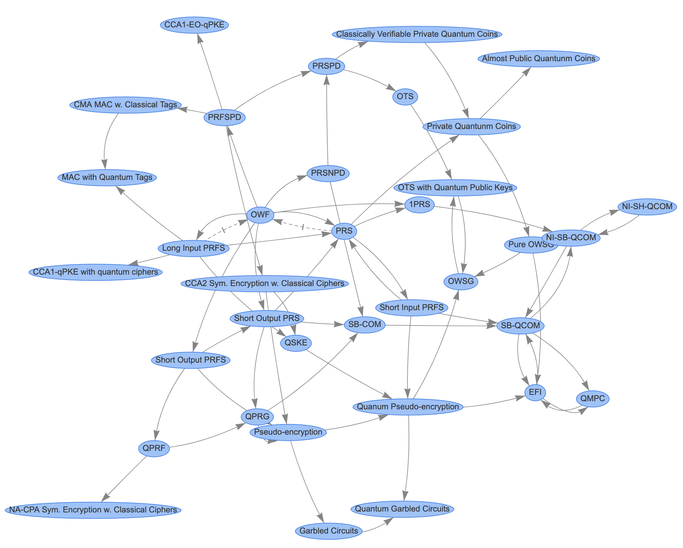
Appendix A Commitments in the CHRS model

This section describes an unconditional bit commitment protocol in the CHRSย model, and follows very closely the approach of [MNY23] to compile a ${\mathsf{1PRS}}$ into a commitment.

We adopt the definition of bit commitment with common reference state from [MNY23] with the slight modification that the reference state must be Haar random. We point out another subtlety about this definition in Remark A.2 below.

Definition A.1 (Bit commitment in the CHRSย model).

A non-interactive bit commitment scheme in the CHRSย model is given by a tuple of QPT algorithms: $C$ (the sender) and $R$ (the receiver). Let $\{\ket{\psi_{n}}\}_{n\in\mathbb{N}}$ denote the family of common Haar random states. The scheme consists of the following two phases.

  • โ€ข

    Commit phase: The sender $C$ takes polynomially many copies of $\ket{\psi_{n}}$ and a bit $b\in\left\{0,1\right\}$ as the input, generates a quantum state on registers $\mathsf{C}$ and $\mathsf{R}$, and sends register $\mathsf{C}$ to the receiver $R$.

  • โ€ข

    Reveal phase: $C$ sends $b$ and register $\mathsf{R}$ to R. R takes polynomially many copies of $\ket{\psi_{n}}$ and $(b,\mathsf{C},\mathsf{R})$ as input, and outputs either $b$ or $\perp$.

Remark A.2.

Note that in the above definition (which follows the style of [MNY23]), for a given security parameter $n$, parties only have access to copies of the Haar random state $\ket{\psi_{n}}$. In contrast, in the definition of CHRS model that we gave in Sectionย 4.1, the entire family $\{\ket{\psi_{n}}\}_{n\in\mathbb{N}}$ is available to all parties (who can request polynomially many copies, in the security parameter $n$). This distinction is important when proving an oracle separation, like our Theoremย 5.1, because there we want to argue about the existence of a primitive relative to a fixed oracle (rather than an oracle that changes for each value of the security parameter). However, this distinction is not as important in this section, given that our ${\mathsf{1PRS}}$ construction, and the resulting commitment scheme, does in fact use only the single state $\ket{\psi_{n}}$ when the security parameter is $n$. So, we elect to use the simpler Definitionย A.1 in this section for simplicity.

Next, we define the notions of hiding and sum-binding for a bit commitment in the CHRSย model, analogously to [CKR16] and [MNY23]. We consider statistical hiding with bounded access to the common Haar random state, and statistical sum-binding against adversaries that have even unbounded access to the state.

Definition A.3 (Polynomial-copy statistical hiding).

A quantum commitment scheme $(C,R)$ in the CHRSย model is said to be polynomial-copy statistically hiding if for any computationally unbounded uniform algorithm $\mathcal{A}$ and for any polynomial $t=t(n)$, there exists a negligible function ${\mathsf{negl}}$ such that, for all $n$,

$\displaystyle\Big{\lvert}\Pr_{\ket{\psi_{n}}\leftarrow\mu_{n}}\Big{[}$ $\displaystyle 1\leftarrow\mathcal{A}\left\lparen 1^{n},\ket{\psi_{n}}^{\otimes t},\operatorname{Tr}_{\mathsf{R}}[\sigma_{\mathsf{C},\mathsf{R}}]\right\rparen:\sigma_{\mathsf{C},\mathsf{R}}\leftarrow C_{\text{com}}(\ket{\psi_{n}}^{\otimes r},0)\Big{]}$
$\displaystyle-\Pr_{\ket{\psi_{n}}\leftarrow\mu_{n}}\left[1\leftarrow\mathcal{A}\left\lparen 1^{n},\ket{\psi_{n}}^{\otimes t},\operatorname{Tr}_{\mathsf{R}}[\sigma_{\mathsf{C},\mathsf{R}}]\right\rparen:\sigma_{\mathsf{C},\mathsf{R}}\leftarrow C_{\text{com}}(\ket{\psi_{n}}^{\otimes r},1)\right]\Big{\rvert}\leq{\mathsf{negl}}(n)$

where $C_{\text{com}}$ is the โ€œcommit phaseโ€ of the sender algorithm $C$, and $r=r(n)$ is the number of copies of the common Haar random state used by $C_{\text{com}}$.

Definition A.4 (Statistical sum-binding).

A commitment scheme $(C,R)$ in the CHRSย model satisfies statistical sum-binding if the following holds. Let $C_{0}^{*}$ and $C_{1}^{*}$ be any computationally unbounded malicious committers that take an unbounded number of copies of $\ket{\psi_{n}}$ as input, and behave identically in the โ€œcommit phaseโ€. Let $p_{b}$ be the probability that $R$ accepts the revealed bit $b$ in an interaction with $C_{b}^{*}$. Then, there exists a negligible function ${\mathsf{negl}}$ such that, for all $n$,

$$p_{0}+p_{1}\leq 1+{\mathsf{negl}}(n).$$

Following the approach in [MNY23], we will show that our commitment scheme satisfies a stronger binding condition, called โ€œextractor-based bindingโ€, first introduced in [AQY22].

Definition A.5 (Statistical extractor-based binding).

A commitment scheme in the CHRSย model $(C,R)$ satisfies statistical extractor-based binding if there is a computationally unbounded algorithm $\mathcal{E}=\left\{\mathcal{E}_{n}\right\}_{n\in\mathbb{N}}$, called the extractor, such that for any unbounded time malicious committer $C^{*}$, the experiments $\mathsf{Real}_{n}^{C^{*}}$ and $\mathsf{Ideal}_{n}^{C^{*},\mathcal{E}}$ are statistically indistinguishable, i.e.ย an unbounded-time distinguisher cannot distinguish the two with non-negligible advantage, where the experiments $\mathsf{Real}_{n}^{C^{*}}$ and $\mathsf{Ideal}_{n}^{C^{*},\mathcal{E}}$ are defined as follows. Let $\{\ket{\psi_{n}}\}_{n\in\mathbb{N}}$ denote the family of common Haar random states.

  • โ€ข

    ๐–ฑ๐–พ๐–บ๐—…nCโˆ—superscriptsubscript๐–ฑ๐–พ๐–บ๐—…๐‘›superscript๐ถ\mathsf{Real}_{n}^{C^{*}}: The malicious committer $C^{*}$ takes polynomially many copies of $\ket{\psi_{n}}$ as input, and interacts with the honest receiver $R$ in the commit and reveal phases. Let $b\in\left\{0,1,\perp\right\}$ be the output of $R$ and $\tau_{C^{*}}$ be the final state of $C^{*}$. The experiment outputs the pair $(\tau_{C^{*}},b)$.

  • โ€ข

    ๐–จ๐–ฝ๐–พ๐–บ๐—…nCโˆ—,โ„ฐsuperscriptsubscript๐–จ๐–ฝ๐–พ๐–บ๐—…๐‘›superscript๐ถโ„ฐ\mathsf{Ideal}_{n}^{C^{*},\mathcal{E}}: $C^{*}$ takes $\ket{\psi_{n}}$ as input and runs its commit phase to generate a commitment $\sigma_{\mathsf{C}}$ where $C^{*}$ may keep a state that is entangled with $\sigma_{\mathsf{C}}$. $\mathcal{E}_{n}$ takes the register $\mathsf{C}$ as input, outputs an extracted bit $b^{*}\in\left\{0,1\right\}$, and sends a post-execution state on $\mathsf{C}$ (which might be different from the original one) to R as a commitment. Then $C^{*}$ and $R$ run the reveal phase. Let $b$ be the output of $R$ and $\tau_{C^{*}}$ be the final state of $C^{*}$. If $b\notin\left\{\perp,b^{*}\right\}$, then the experiment outputs a symbol fail and otherwise outputs a tuple $(\tau_{C^{*}},b)$.

Morimae, Nehoran, and Yamakawa show the following result:

Lemma A.6 ([MNY23, Lemma 7.6]).

Statistical extractor-based binding implies statistical sum-binding.

Our commitment protocol in the CHRS model takes essentially the same form as that in [MNY23]. Let $\{\ket{\phi_{k}}\}_{k}$ be an ${\mathsf{1PRS}}$ in the CHRS model. Let $\mathsf{R}$ and $\mathsf{C}$ be registers of the same size as $\ket{\phi_{k}}$. Then, to commit to 00, the sender prepares

$$\sum_{k}(\ket{k}\ket{0})_{\mathsf{R}}\ket{\phi_{k}}_{\mathsf{C}}\,.$$

To commit to $1$, the sender prepares

$$\sum_{x}\ket{x}_{\mathsf{R}}\ket{x}_{\mathsf{C}}\,,$$

i.e.ย the maximally entangled state across $\mathsf{R}$ and $\mathsf{C}$.

Substituting our ${\mathsf{1PRS}}$ from Fig.ย 2, we get the following construction, where the base commitment is repeated in parallel, and the reveal phase is carried out by using SWAP tests.

Commitment phase: the sender takes as input a bit $b\in\left\{0,1\right\}$. Let $$\ket{\Psi_{0}}_{\mathsf{R},\mathsf{C}}=\sum_{a,b\in\left\{0,1\right\}^{0.45n}}\ket{ab\|0^{0.1n}}_{\mathsf{R}}X^{a}Z^{b}\ket{\psi_{n}}_{\mathsf{C}}\,,$$ and let $$\ket{\Psi_{1}}_{\mathsf{R},\mathsf{C}}=\sum_{x\in\{0,1\}^{n}}\ket{x}_{\mathsf{R}}\ket{x}_{\mathsf{C}}\,.$$ The sender prepares $\ket{\Psi_{b}}^{\otimes n}_{\mathsf{C}_{1}\ldots\mathsf{C}_{n},\mathsf{R}_{1}\ldots\mathsf{R}_{n}}$, and sends registers $\mathsf{C}_{1}\ldots\mathsf{C}_{n}$ to the receiver. Reveal phase: The sender sends $b$ and registers $\mathsf{R}_{1}\ldots\mathsf{R}_{n}$ to the receiver. The receiver prepares the state $\ket{\Psi_{b}}^{\otimes n}_{\mathsf{C}^{\prime}_{1}\ldots\mathsf{C}^{\prime}_{n},\mathsf{R}^{\prime}_{1}\ldots\mathsf{R}^{\prime}_{n}}$, and performs a SWAP test between registers $(\mathsf{C}_{1}\ldots\mathsf{C}_{n},\mathsf{R}_{1}\ldots\mathsf{R}_{n})$ and $(\mathsf{C}^{\prime}_{1}\ldots\mathsf{C}^{\prime}_{n},\mathsf{R}^{\prime}_{1}\ldots\mathsf{R}^{\prime}_{n})$, and accepts if and only if all of the SWAP tests output 1.
Figure 4: Quantum bit commitment scheme in the CHRSย model
Theorem A.7.

The protocol in Fig.ย 4 satisfies polynomial-copy statistical hiding (as in Definitionย A.3) and statistical extractor-based binding (as in Definitionย A.5).

Remark A.8.

Notice that, since a commitment scheme in the plain model cannot be both statistically binding and hiding [LC97, May97], we also cannot, in the CHRSย model, simultaneously achieve statistical binding and $t$-copy statistical hiding for $t$ exponentially large in $n$. This is because when $t$ is exponentially large, an unbounded adversary can learn the common Haar random state $\ket{\psi_{n}}$ entirely via tomography. Hence, in this case, $t$-copy statistical hiding is equivalent to statistical hiding in the plain model.

Proof of Theoremย A.7.

Polynomial-copy statistical hiding. The $\mathsf{C}$ registers of $\ket{\Psi_{0}}$ and $\ket{\Psi_{1}}$ are respectively in the state $\rho_{0}=\operatorname{Tr}_{\mathsf{R}}\ket{\Psi_{0}}\bra{\Psi_{0}}=\frac{1}{2^{0.9n}}\sum_{a,b}{X^{a}Z^{b}\ket{\psi_{n}}\bra{\psi_{n}}X^{a}Z^{b}}$ and $\rho_{1}=\operatorname{Tr}_{\mathsf{R}}\ket{\Psi_{1}}\bra{\Psi_{1}}=\frac{1}{2^{n}}\sum_{x}\ket{x}\bra{x}$. These two states are indistinguishable even to an adversary with a polynomial number of copies of $\ket{\psi_{n}}$. In fact, using Corollaryย 4.12, we have that for any $t=\operatorname{poly}(n)$, there is negligible function ${\mathsf{negl}}$, such that for all $n$,

$$\left\lVert{\rho_{0}^{\otimes n}\otimes\psi^{\otimes t}-\rho_{1}^{\otimes n}\otimes\psi^{\otimes t}}\right\rVert\leq n\left\lVert{\rho_{0}\otimes\psi^{\otimes t}-\rho_{1}\otimes\psi^{\otimes t}}\right\rVert={\mathsf{negl}}(n)$$

Statistical extractor-based binding.

$\mathsf{Real}_{n}^{C^{*}}$: 1. $C^{*}$ takes polynomially many copies of $\ket{\psi_{n}}$ as input and generates a state $\ket{\phi_{b}}$ over registers $(\mathsf{C},\mathsf{R},\mathsf{W})$ along with a bit $b\in\{0,1\}$ where $\mathsf{W}$ is the work register of $C^{*}$. 2. $C^{*}$ sends $\mathsf{C}$ to $R$ in the commit phase. 3. $C^{*}$ sends $(b,\mathsf{R})$ to $R$ in the reveal phase. 4. $R$ runs the verification in the reveal phase. That is, $R$ takes as input $\ket{\psi_{n}}^{\otimes n}_{\mathsf{C}^{\prime}}$, and $(b,\mathsf{C},\mathsf{R})$ from $C^{*}$; it prepares an ancilla register $\mathsf{V}$ in the state $\ket{0\dots 0}_{\mathsf{V}}$, applies the projective measurement $(P_{b},\mathds{1}-P_{b})$ on registers $(\mathsf{C}^{\prime},\mathsf{C},\mathsf{R},\mathsf{V})$. 5. If $R$ rejects (i.e.ย R๐‘…R obtains the outcome corresponding to $\mathds{1}-P_{b}$), $b$ is replaced by $\perp$. 6. The experiment outputs $(b,\mathsf{W})$. $\mathsf{Ideal}^{C^{*},\mathcal{E}}$: 1. $C^{*}$ takes polynomially many copies of $\ket{\psi_{n}}$ as input and generates a state $\ket{\phi_{b}}$ over registers $(\mathsf{C},\mathsf{R},\mathsf{W})$ along with a bit $b\in\{0,1\}$ where $\mathsf{W}$ is the work register of $C^{*}$. 2. $C^{*}$ sends $\mathsf{C}$ to $R$ in the commit phase. 3. The extractor $\mathcal{E}_{n}$ prepares the ancilla register $\mathsf{E}$ in the state $\ket{0\dots 0}_{\mathsf{E}}$, applies the projective measurement {ฮ ~0,ฮ ~1,ฮ ~โŸ‚}subscript~ฮ 0subscript~ฮ 1subscript~ฮ perpendicular-to\{\tilde{\Pi}_{0},\tilde{\Pi}_{1},\tilde{\Pi}_{\perp}\} on registers $\mathsf{C}$ and $\mathsf{E}$, and lets $b^{*}\in\{0,1,\perp\}$ be the outcome. $\mathcal{E}_{n}$ sends $\mathsf{C}$ to $R$. 4. $C^{*}$ sends $(b,\mathsf{R})$ to $R$. 5. $R$ runs the verification in the reveal phase. That is, $R$ takes as input $\ket{\psi_{n}}^{\otimes n}_{\mathsf{C}^{\prime}}$, and $(b,\mathsf{C},\mathsf{R})$ from $C^{*}$; it prepares an ancilla register $\mathsf{V}$ in the state $\ket{0\dots 0}_{\mathsf{V}}$, applies the projective measurement $(P_{b},\mathds{1}-P_{b})$ on registers $(\mathsf{C}^{\prime},\mathsf{C},\mathsf{R},\mathsf{V})$. 6. If $R$ accepts (i.e.ย R๐‘…R obtains the outcome corresponding to $P_{b}$) and bโ‰ bโˆ—๐‘superscript๐‘b\neq b^{*}, the experiment outputs the special symbol $\mathsf{fail}$ and halts. 7. If $R$ rejects (i.e.ย R๐‘…R obtains the outcome corresponding to $\mathds{1}-P_{b}$), $b$ is replaced by $\perp$. 8. The experiment outputs $(b,\mathsf{W})$.
Figure 5: $\mathsf{Real}_{n}^{C^{*}}$ and $\mathsf{Ideal}_{n}^{C^{*},\mathcal{E}}$

To show that the construction satisfies the statistical extractor-based binding property we need two technical lemmas.

Lemma A.9 ([HM13, Lemma 2]).

Let $m\in\mathbb{N}$. Let $\rho$ be a quantum state over $m$ registers ๐– 1,โ€ฆ,๐– msubscript๐– 1โ€ฆsubscript๐– ๐‘š\mathsf{A}_{1},\dots,\mathsf{A}_{m}. Let $\sigma$ be a quantum state over $m$ registers $\mathsf{B}_{1},\dots,\mathsf{B}_{m}$. Consider the following test, applied to $\rho\otimes\sigma$:

  1. 1.

    For each $i\in[m]$, do the SWAP test between ๐– isubscript๐– ๐‘–\mathsf{A}_{i} and $\mathsf{B}_{i}$.

  2. 2.

    Accept if all SWAP tests are successful

Then the success probability that the above test accepts is $\frac{1}{2^{m}}\sum_{S\subseteq[m]}\operatorname{Tr}[\rho_{S}\sigma_{S}]$, where $\rho_{S}$ is the state obtained by tracing out all registers ๐– isubscript๐– ๐‘–\mathsf{A}_{i} of $\rho$ such that $i\notin S$, and $\sigma_{S}$ is the state obtained by tracing out all registers $\mathsf{B}_{i}$ of $\sigma$ such that $i\notin S$.

Lemma A.10 ([Yan22, Lemma 31]).

Let $\ket{\Psi_{0}}_{\mathsf{X},\mathsf{Y}}$ and $\ket{\Psi_{1}}_{\mathsf{X},\mathsf{Y}}$ be pure states over registers $(\mathsf{X},\mathsf{Y})$ such that

$$F\left(\operatorname{Tr}_{\mathsf{Y}}[\ket{\Psi_{0}}\bra{\Psi_{0}}_{\mathsf{X},\mathsf{Y}}],\operatorname{Tr}_{\mathsf{Y}}[\ket{\Psi_{1}}\bra{\Psi_{1}}_{\mathsf{X}.\mathsf{Y}}]\right)=\epsilon$$

Then there is a projective measurement {ฮ 0,ฮ 1,ฮ โŸ‚โ‰”๐Ÿ™โˆ’ฮ 0โˆ’ฮ 1}โ‰”subscriptฮ 0subscriptฮ 1subscriptฮ perpendicular-to1subscriptฮ 0subscriptฮ 1\{\Pi_{0},\Pi_{1},\Pi_{\perp}\coloneqq\mathds{1}-\Pi_{0}-\Pi_{1}\} over registers $\mathsf{X}$ such that for each $b\in\{0,1\}$,

โˆฅ(ฮ b)๐–ทโŠ—๐Ÿ™๐–ธโ€‹|ฮจbโŸฉ๐–ท,๐–ธโˆฅ2โ‰ฅ1โˆ’2โ€‹ฯตsuperscriptdelimited-โˆฅโˆฅtensor-productsubscriptsubscriptฮ ๐‘๐–ทsubscript1๐–ธsubscriptketsubscriptฮจ๐‘๐–ท๐–ธ212italic-ฯต\left\lVert{(\Pi_{b})_{\mathsf{X}}\otimes\mathds{1}_{\mathsf{Y}}\ket{\Psi_{b}}_{\mathsf{X},\mathsf{Y}}}\right\rVert^{2}\geq 1-\sqrt{2\epsilon}

Recall that we defined the reduced state of the honest commitment states $\ket{\Psi_{0}}_{\mathsf{C}\mathsf{R}}$ and $\ket{\Psi_{1}}_{\mathsf{C}\mathsf{R}}$ on the $\mathsf{C}$ registers respectively as $\rho_{0}=\operatorname{Tr}_{\mathsf{R}}\ket{\Psi_{0}}\bra{\Psi_{0}}=\frac{1}{2^{0.9n}}\sum_{a,b}{X^{a}Z^{b}\ket{\psi_{n}}\bra{\psi_{n}}X^{a}Z^{b}}$ and $\rho_{1}=\operatorname{Tr}_{\mathsf{R}}[\ket{\Psi_{1}}\bra{\Psi_{1}}]=\frac{1}{2^{n}}\sum_{x}\ket{x}\bra{x}$.

Since the rank of $\rho_{0}$ does not exceed $2^{0.9n}$, while $\rho_{1}=\frac{\mathds{1}}{2^{n}}$, it is straightforward to show that $\left\lVert{\rho_{0}-\rho_{1}}\right\rVert\geq 1-\frac{2^{0.9n}}{2^{n}}=1-{\mathsf{negl}}(n)$ (by taking the eigendecomposition of $\rho_{0}$). Set $\epsilon=1-\left\lVert{\rho_{0}-\rho_{1}}\right\rVert={\mathsf{negl}}(n)$. According to Lemmaย A.10, there exists a family of orthogonal projectors {ฮ 0,ฮ 1,ฮ โŸ‚=๐Ÿ™โˆ’ฮ 0โˆ’ฮ 1}subscriptฮ 0subscriptฮ 1subscriptฮ perpendicular-to1subscriptฮ 0subscriptฮ 1\left\{\Pi_{0},\Pi_{1},\Pi_{\perp}=\mathds{1}-\Pi_{0}-\Pi_{1}\right\} on $\mathsf{C}$ such that for each $b\in\left\{0,1\right\}$, it holds that

โˆฅ(๐Ÿ™โˆ’ฮ b)๐–ขโŠ—๐Ÿ™๐–ฑโ€‹|ฮจbโŸฉโˆฅ2โ‰ค2โ€‹ฯต.superscriptdelimited-โˆฅโˆฅtensor-productsubscript1subscriptฮ ๐‘๐–ขsubscript1๐–ฑketsubscriptฮจ๐‘22italic-ฯต\left\lVert{(\mathds{1}-\Pi_{b})_{\mathsf{C}}\otimes\mathds{1}_{\mathsf{R}}\ket{\Psi_{b}}}\right\rVert^{2}\leq\sqrt{2\epsilon}\,. (17)

We define the extractor $\mathcal{E}_{n}$ as follows:

  • โ€ข

    Upon receiving the commitment register $\mathsf{C}=(\mathsf{C}_{1},\dots,\mathsf{C}_{n})$, for each $i\in[n]$, apply the projective measurement {ฮ 0,ฮ 1,ฮ โŸ‚}subscriptฮ 0subscriptฮ 1subscriptฮ perpendicular-to\left\{\Pi_{0},\Pi_{1},\Pi_{\perp}\right\} on $\mathsf{C}_{i}$ to obtain an outcome $b_{i}\in\left\{0,1,\perp\right\}$.

  • โ€ข
    • โ€“

      If $\left\lvert\left\{i\in[n]:b_{i}=0\right\}\right\rvert>2n/3$, output $b^{*}=0$.

    • โ€“

      If $\left\lvert\left\{i\in[n]:b_{i}=1\right\}\right\rvert>2n/3$, output $b^{*}=1$.

    • โ€“

      Otherwise, output $b^{*}=\perp$

We can equivalently describe $\mathcal{E}_{n}$ as some projective measurement {ฮ ~0,ฮ ~1,ฮ ~โŸ‚}subscript~ฮ 0subscript~ฮ 1subscript~ฮ perpendicular-to\left\{\tilde{\Pi}_{0},\tilde{\Pi}_{1},\tilde{\Pi}_{\perp}\right\} on register $\mathsf{C}$ and an ancilla register $\mathsf{E}$ initialized as $\ket{0\ldots 0}_{\mathsf{E}}$.

For $b\in\left\{0,1\right\}$, let $(P_{b},\mathds{1}-P_{b})$ be the projective measurement corresponding to the โ€œpurifiedโ€ verification performed by the receiver $R$ in the reveal phase. That is, $(P_{b},\mathds{1}-P_{b})$ is defined so that $R$ is described as follows: on input $\ket{\psi_{n}}^{\otimes n}_{\mathsf{C}^{\prime}}$, where $\mathsf{C}^{\prime}\coloneqq\mathsf{C}^{\prime}_{1}\ldots\mathsf{C}^{\prime}_{n}$, as well as $(b,\mathsf{C},\mathsf{R})$ from the sender, $R$ initializes an ancilla register $\mathsf{V}$ to $\ket{0\dots 0}_{\mathsf{V}}$, and applies the projective measurement $(P_{b},\mathds{1}-P_{b})$ to all previous registers. $R$ accepts if the outcome is the former, and rejects if its the latter.

Let $C^{*}$ be a malicious sender. Then, concretely, the experiments $\mathsf{Real}_{n}^{C^{*}}$ and $\mathsf{Ideal}_{n}^{C^{*},\mathcal{E}}$ are as in Fig.ย 5.

In what follows, for simplicity, we omit writing identities on registers were operators act trivially. Let $\ket{\phi_{b}}$ be defined as in Fig.ย 5. We define the mixed states $\rho_{\mathsf{real}}(b)$ and $\rho_{\mathsf{ideal}}(b)$ to correspond to the outputs of $\mathsf{Real}_{n}^{C*}$ and $\mathsf{Ideal}_{n}^{C^{*},\mathcal{E}}$ conditioned on the bit sent from $C^{*}$ being $b$. That is, we let252525To see that these are the correct definitions one can use the ciclicity of the partial trace.

$$\rho_{\mathsf{real}}(b)\coloneqq\operatorname{Tr}_{\mathsf{C}^{\prime},\mathsf{C},\mathsf{R},\mathsf{V},\mathsf{E}}[P_{b}\ket{\tilde{\phi_{b}}}\bra{\tilde{\phi_{b}}}]\otimes\ket{b}\bra{b}+\operatorname{Tr}_{\mathsf{C}^{\prime},\mathsf{C},\mathsf{R},\mathsf{V},\mathsf{E}}[(\mathds{1}-P_{b})\ket{\tilde{\phi_{b}}}\bra{\tilde{\phi_{b}}}]\otimes\ket{\perp}\bra{\perp}$$ (18)

and

$\displaystyle\rho_{\mathsf{ideal}}(b)\coloneqq$ $\displaystyle\operatorname{Tr}_{\mathsf{C}^{\prime},\mathsf{C},\mathsf{R},\mathsf{V},\mathsf{E}}[N_{b}\ket{\tilde{\phi_{b}}}\bra{\tilde{\phi_{b}}}]\otimes\ket{b}\bra{b}+\operatorname{Tr}_{\mathsf{C}^{\prime},\mathsf{C},\mathsf{R},\mathsf{V},\mathsf{E}}[N_{\perp}\ket{\tilde{\phi_{b}}}\bra{\tilde{\phi_{b}}}]\otimes\ket{\perp}\bra{\perp}$ (19)
$\displaystyle+\operatorname{Tr}_{\mathsf{C}^{\prime},\mathsf{C},\mathsf{R},\mathsf{V},\mathsf{E}}[N_{\texttt{fail}}\ket{\tilde{\phi_{b}}}\bra{\tilde{\phi_{b}}}]\otimes\ket{\texttt{fail}}\bra{\texttt{fail}}$

where

$$\ket{\tilde{\phi}_{b}}\coloneqq\ket{\phi_{b}}_{\mathsf{C},\mathsf{R},\mathsf{W}}\otimes\ket{\psi_{n}}_{\mathsf{C}^{\prime}}^{\otimes n}\otimes\ket{0\dots 0}_{\mathsf{V}}\otimes\ket{0\dots 0}_{\mathsf{E}}$$

and

Nbโ‰”ฮ ~bโ€‹Pbโ€‹ฮ ~b,Nfailโ‰”(๐Ÿ™โˆ’ฮ ~b)โ€‹Pbโ€‹(๐Ÿ™โˆ’ฮ ~b),NโŸ‚โ‰”๐Ÿ™โˆ’Nbโˆ’Nfail.formulae-sequenceโ‰”subscript๐‘๐‘subscript~ฮ ๐‘subscript๐‘ƒ๐‘subscript~ฮ ๐‘formulae-sequenceโ‰”subscript๐‘fail1subscript~ฮ ๐‘subscript๐‘ƒ๐‘1subscript~ฮ ๐‘โ‰”subscript๐‘perpendicular-to1subscript๐‘๐‘subscript๐‘failN_{b}\coloneqq\tilde{\Pi}_{b}P_{b}\tilde{\Pi}_{b},\,N_{\texttt{fail}}\coloneqq(\mathds{1}-\tilde{\Pi}_{b})P_{b}(\mathds{1}-\tilde{\Pi}_{b}),\,N_{\perp}\coloneqq\mathds{1}-N_{b}-N_{\texttt{fail}}.

Noting that the distribution of $b$ is identical in both experiments, it suffices to prove

$$\left\lVert{\rho_{\mathsf{real}}(b)-\rho_{\mathsf{ideal}}(b)}\right\rVert={\mathsf{negl}}(n)$$

for $b\in\left\{0,1\right\}$. We show the following lemma.

Lemma A.11.

For each $b\in\left\{0,1\right\}$, it holds that

โˆฅ(Pb)๐–ข,๐–ฑ,๐–ขโ€ฒ,๐–ตโ€‹(๐Ÿ™โˆ’ฮ ~b)๐–ข,๐–คโ€‹|ฯ•~bโŸฉโˆฅ2=๐—‡๐–พ๐—€๐—…โ€‹(n).superscriptdelimited-โˆฅโˆฅsubscriptsubscript๐‘ƒ๐‘๐–ข๐–ฑsuperscript๐–ขโ€ฒ๐–ตsubscript1subscript~ฮ ๐‘๐–ข๐–คketsubscript~italic-ฯ•๐‘2๐—‡๐–พ๐—€๐—…๐‘›\left\lVert{(P_{b})_{\mathsf{C},\mathsf{R},\mathsf{C}^{\prime},\mathsf{V}}(\mathds{1}-\tilde{\Pi}_{b})_{\mathsf{C},\mathsf{E}}\ket{\tilde{\phi}_{b}}}\right\rVert^{2}={\mathsf{negl}}(n)\,.
Proof.

By definition of $P_{b}$ and $\ket{\tilde{\phi}_{b}}$, โˆฅPbโ€‹(๐Ÿ™โˆ’ฮ ~b)โ€‹|ฯ•~bโŸฉโˆฅ2superscriptdelimited-โˆฅโˆฅsubscript๐‘ƒ๐‘1subscript~ฮ ๐‘ketsubscript~italic-ฯ•๐‘2\left\lVert{P_{b}(\mathds{1}-\tilde{\Pi}_{b})\ket{\tilde{\phi}_{b}}}\right\rVert^{2} is the probability that the bit extracted from $\ket{\tilde{\phi}_{b}}$ is not $b$ and the residual state passes the verification performed by $R$ with respect to $b$. Let ฯ๐–ข,๐–ฑโ‰”Tr๐–ถ,๐–คโก[(๐Ÿ™โˆ’ฮ ~b)๐–ข,๐–คโ€‹|ฯ•bโŸฉโ€‹โŸจฯ•b|๐–ข,๐–ฑ,๐–ถโŠ—|0โ€‹โ€ฆโ€‹0โŸฉโ€‹โŸจ0โ€‹โ€ฆโ€‹0|๐–ค]โ‰”subscript๐œŒ๐–ข๐–ฑsubscriptTr๐–ถ๐–คtensor-productsubscript1subscript~ฮ ๐‘๐–ข๐–คketsubscriptitalic-ฯ•๐‘subscriptbrasubscriptitalic-ฯ•๐‘๐–ข๐–ฑ๐–ถket0โ€ฆ0subscriptbra0โ€ฆ0๐–ค\rho_{\mathsf{C},\mathsf{R}}\coloneqq\operatorname{Tr}_{\mathsf{W},\mathsf{E}}\left[(\mathds{1}-\tilde{\Pi}_{b})_{\mathsf{C},\mathsf{E}}\ket{\phi_{b}}\bra{\phi_{b}}_{\mathsf{C},\mathsf{R},\mathsf{W}}\otimes\ket{0\dots 0}\bra{0\dots 0}_{\mathsf{E}}\right]. By Lemmaย A.9, this probability is equal to

$$\frac{1}{2^{n}}\sum_{S\subseteq[n]}\operatorname{Tr}[\rho_{S}\sigma_{S}]$$

where $\sigma\coloneqq\bigotimes_{i\in[n]}\ket{\Psi_{b}}\bra{\Psi_{b}}$. Here $\rho_{S}$ and $\sigma_{S}$ are the states obtained by tracing out all $\mathsf{C}_{i}\mathsf{R}_{i}$, respectively $\mathsf{C}^{\prime}_{i}\mathsf{R}^{\prime}_{i}$, for $i\notin S$. Notice that the latter expression for the probability takes into account the fact that $\rho$ is sub-normalized.

By the definition of ฮ ~bsubscript~ฮ ๐‘\tilde{\Pi}_{b}, we can write

ฯ=โˆ‘TโІ[n],|T|โ‰ค2โ€‹n/3Tr๐–ถโก[ฮ ^b(T)โ€‹|ฯ•bโŸฉโ€‹โŸจฯ•b|โ€‹ฮ ^b(T)]๐œŒsubscriptformulae-sequence๐‘‡delimited-[]๐‘›๐‘‡2๐‘›3subscriptTr๐–ถsuperscriptsubscript^ฮ ๐‘๐‘‡ketsubscriptitalic-ฯ•๐‘brasubscriptitalic-ฯ•๐‘superscriptsubscript^ฮ ๐‘๐‘‡\rho=\sum_{T\subseteq[n],|T|\leq 2n/3}\operatorname{Tr}_{\mathsf{W}}\left[{\hat{\Pi}_{b}^{(T)}}\ket{\phi_{b}}\bra{\phi_{b}}\hat{\Pi}_{b}^{(T)}\right]

where

ฮ ^b(T)=(โจ‚iโˆˆT(ฮ b)๐–ขi)โŠ—(โจ‚iโˆ‰T(๐Ÿ™โˆ’ฮ b)๐–ขi).superscriptsubscript^ฮ ๐‘๐‘‡tensor-productsubscripttensor-product๐‘–๐‘‡subscriptsubscriptฮ ๐‘subscript๐–ข๐‘–subscripttensor-product๐‘–๐‘‡subscript1subscriptฮ ๐‘subscript๐–ข๐‘–\hat{\Pi}_{b}^{(T)}=\left\lparen\bigotimes_{i\in T}(\Pi_{b})_{\mathsf{C}_{i}}\right\rparen\otimes\left\lparen\bigotimes_{i\notin T}(\mathds{1}-\Pi_{b})_{\mathsf{C}_{i}}\right\rparen\,.

We have

$\displaystyle\frac{1}{2^{n}}$ $\displaystyle\sum_{S\subseteq[n]}\operatorname{Tr}\left[\rho_{S}\sigma_{S}\right]$
=12nโ€‹โˆ‘SโІ[n]โˆ‘TโІ[n]:|T|โ‰ค2โ€‹n/3Trโก[(Tr{๐–ขi,๐–ฑi}iโˆ‰S,๐–ถโกฮ ^b(T)โ€‹|ฯ•bโŸฉโ€‹โŸจฯ•b|โ€‹ฮ b^(T))โ€‹(โจ‚iโˆˆS|ฮจbโŸฉโ€‹โŸจฮจb|๐–ขi,๐–ฑi)].absent1superscript2๐‘›subscript๐‘†delimited-[]๐‘›subscript:๐‘‡delimited-[]๐‘›๐‘‡2๐‘›3TrsubscriptTrsubscriptsubscript๐–ข๐‘–subscript๐–ฑ๐‘–๐‘–๐‘†๐–ถsuperscriptsubscript^ฮ ๐‘๐‘‡ketsubscriptitalic-ฯ•๐‘brasubscriptitalic-ฯ•๐‘superscript^subscriptฮ ๐‘๐‘‡subscripttensor-product๐‘–๐‘†ketsubscriptฮจ๐‘subscriptbrasubscriptฮจ๐‘subscript๐–ข๐‘–subscript๐–ฑ๐‘–\displaystyle=\frac{1}{2^{n}}\sum_{S\subseteq[n]}\sum_{T\subseteq[n]:|T|\leq 2n/3}\operatorname{Tr}\left[\left\lparen\operatorname{Tr}_{\left\{\mathsf{C}_{i},\mathsf{R}_{i}\right\}_{i\notin S},\mathsf{W}}\hat{\Pi}_{b}^{(T)}\ket{\phi_{b}}\bra{\phi_{b}}\hat{\Pi_{b}}^{(T)}\right\rparen\left\lparen\bigotimes_{i\in S}\ket{\Psi_{b}}\bra{\Psi_{b}}_{\mathsf{C}_{i},\mathsf{R}_{i}}\right\rparen\right]\,.

Now, for any $S$ and $T$, we have

Trโก[(Tr{๐–ขi,๐–ฑi}iโˆ‰S,๐–ถโกฮ ^b(T)โ€‹|ฯ•bโŸฉโ€‹โŸจฯ•b|โ€‹ฮ b^(T))โ€‹(โจ‚iโˆˆS|ฮจbโŸฉโ€‹โŸจฮจb|๐–ขi,๐–ฑi)]TrsubscriptTrsubscriptsubscript๐–ข๐‘–subscript๐–ฑ๐‘–๐‘–๐‘†๐–ถsuperscriptsubscript^ฮ ๐‘๐‘‡ketsubscriptitalic-ฯ•๐‘brasubscriptitalic-ฯ•๐‘superscript^subscriptฮ ๐‘๐‘‡subscripttensor-product๐‘–๐‘†ketsubscriptฮจ๐‘subscriptbrasubscriptฮจ๐‘subscript๐–ข๐‘–subscript๐–ฑ๐‘–\displaystyle\operatorname{Tr}\left[\left\lparen\operatorname{Tr}_{\left\{\mathsf{C}_{i},\mathsf{R}_{i}\right\}_{i\notin S},\mathsf{W}}\hat{\Pi}_{b}^{(T)}\ket{\phi_{b}}\bra{\phi_{b}}\hat{\Pi_{b}}^{(T)}\right\rparen\left\lparen\bigotimes_{i\in S}\ket{\Psi_{b}}\bra{\Psi_{b}}_{\mathsf{C}_{i},\mathsf{R}_{i}}\right\rparen\right]
$\displaystyle=$ Trโก[((๐Ÿ™โˆ’ฮ b){๐–ขi}iโˆˆS\TโŠ—|S\T|โ€‹(Tr{๐–ขi,๐–ฑi}iโˆ‰S,๐–ถโกฮ ^b(T)โ€‹|ฯ•bโŸฉโ€‹โŸจฯ•b|โ€‹ฮ b^(T))โ€‹(๐Ÿ™โˆ’ฮ b){๐–ขi}iโˆˆS\TโŠ—|S\T|)โ€‹(โจ‚iโˆˆS|ฮจbโŸฉโ€‹โŸจฮจb|๐–ขi,๐–ฑi)]Trsubscriptsuperscript1subscriptฮ ๐‘tensor-productabsent\๐‘†๐‘‡subscriptsubscript๐–ข๐‘–๐‘–\๐‘†๐‘‡subscriptTrsubscriptsubscript๐–ข๐‘–subscript๐–ฑ๐‘–๐‘–๐‘†๐–ถsuperscriptsubscript^ฮ ๐‘๐‘‡ketsubscriptitalic-ฯ•๐‘brasubscriptitalic-ฯ•๐‘superscript^subscriptฮ ๐‘๐‘‡subscriptsuperscript1subscriptฮ ๐‘tensor-productabsent\๐‘†๐‘‡subscriptsubscript๐–ข๐‘–๐‘–\๐‘†๐‘‡subscripttensor-product๐‘–๐‘†ketsubscriptฮจ๐‘subscriptbrasubscriptฮจ๐‘subscript๐–ข๐‘–subscript๐–ฑ๐‘–\displaystyle\operatorname{Tr}\left[\left\lparen(\mathds{1}-\Pi_{b})^{\otimes|S\backslash T|}_{\left\{\mathsf{C}_{i}\right\}_{i\in S\backslash T}}\left\lparen\operatorname{Tr}_{\left\{\mathsf{C}_{i},\mathsf{R}_{i}\right\}_{i\notin S},\mathsf{W}}\hat{\Pi}_{b}^{(T)}\ket{\phi_{b}}\bra{\phi_{b}}\hat{\Pi_{b}}^{(T)}\right\rparen(\mathds{1}-\Pi_{b})^{\otimes|S\backslash T|}_{\left\{\mathsf{C}_{i}\right\}_{i\in S\backslash T}}\right\rparen\left\lparen\bigotimes_{i\in S}\ket{\Psi_{b}}\bra{\Psi_{b}}_{\mathsf{C}_{i},\mathsf{R}_{i}}\right\rparen\right]
$\displaystyle=$ Trโก[(Tr{๐–ขi,๐–ฑi}iโˆ‰S,๐–ถโกฮ ^b(T)โ€‹|ฯ•bโŸฉโ€‹โŸจฯ•b|โ€‹ฮ b^(T))โ€‹(๐Ÿ™โˆ’ฮ b){๐–ขi}iโˆˆS\TโŠ—|S\T|โ€‹(โจ‚iโˆˆS|ฮจbโŸฉโ€‹โŸจฮจb|๐–ขi,๐–ฑi)โ€‹(๐Ÿ™โˆ’ฮ b){๐–ขi}iโˆˆS\TโŠ—|S\T|]TrsubscriptTrsubscriptsubscript๐–ข๐‘–subscript๐–ฑ๐‘–๐‘–๐‘†๐–ถsuperscriptsubscript^ฮ ๐‘๐‘‡ketsubscriptitalic-ฯ•๐‘brasubscriptitalic-ฯ•๐‘superscript^subscriptฮ ๐‘๐‘‡subscriptsuperscript1subscriptฮ ๐‘tensor-productabsent\๐‘†๐‘‡subscriptsubscript๐–ข๐‘–๐‘–\๐‘†๐‘‡subscripttensor-product๐‘–๐‘†ketsubscriptฮจ๐‘subscriptbrasubscriptฮจ๐‘subscript๐–ข๐‘–subscript๐–ฑ๐‘–subscriptsuperscript1subscriptฮ ๐‘tensor-productabsent\๐‘†๐‘‡subscriptsubscript๐–ข๐‘–๐‘–\๐‘†๐‘‡\displaystyle\operatorname{Tr}\left[\left\lparen\operatorname{Tr}_{\left\{\mathsf{C}_{i},\mathsf{R}_{i}\right\}_{i\notin S},\mathsf{W}}\hat{\Pi}_{b}^{(T)}\ket{\phi_{b}}\bra{\phi_{b}}\hat{\Pi_{b}}^{(T)}\right\rparen(\mathds{1}-\Pi_{b})^{\otimes|S\backslash T|}_{\left\{\mathsf{C}_{i}\right\}_{i\in S\backslash T}}\left\lparen\bigotimes_{i\in S}\ket{\Psi_{b}}\bra{\Psi_{b}}_{\mathsf{C}_{i},\mathsf{R}_{i}}\right\rparen(\mathds{1}-\Pi_{b})^{\otimes|S\backslash T|}_{\left\{\mathsf{C}_{i}\right\}_{i\in S\backslash T}}\right]
$\displaystyle\leq$ โˆฅฮ ^bโ€‹|ฯ•bโŸฉโˆฅ2โ€‹Trโก[(๐Ÿ™โˆ’ฮ b){๐–ขi}iโˆˆS\TโŠ—|S\T|โ€‹(โจ‚iโˆˆS|ฮจbโŸฉโ€‹โŸจฮจb|๐–ขi,๐–ฑi)โ€‹(๐Ÿ™โˆ’ฮ b){๐–ขi}iโˆˆS\TโŠ—|S\T|]superscriptdelimited-โˆฅโˆฅsubscript^ฮ ๐‘ketsubscriptitalic-ฯ•๐‘2Trsubscriptsuperscript1subscriptฮ ๐‘tensor-productabsent\๐‘†๐‘‡subscriptsubscript๐–ข๐‘–๐‘–\๐‘†๐‘‡subscripttensor-product๐‘–๐‘†ketsubscriptฮจ๐‘subscriptbrasubscriptฮจ๐‘subscript๐–ข๐‘–subscript๐–ฑ๐‘–subscriptsuperscript1subscriptฮ ๐‘tensor-productabsent\๐‘†๐‘‡subscriptsubscript๐–ข๐‘–๐‘–\๐‘†๐‘‡\displaystyle\left\lVert{\hat{\Pi}_{b}\ket{\phi_{b}}}\right\rVert^{2}\operatorname{Tr}\left[(\mathds{1}-\Pi_{b})^{\otimes|S\backslash T|}_{\left\{\mathsf{C}_{i}\right\}_{i\in S\backslash T}}\left\lparen\bigotimes_{i\in S}\ket{\Psi_{b}}\bra{\Psi_{b}}_{\mathsf{C}_{i},\mathsf{R}_{i}}\right\rparen(\mathds{1}-\Pi_{b})^{\otimes|S\backslash T|}_{\left\{\mathsf{C}_{i}\right\}_{i\in S\backslash T}}\right]
$\displaystyle\leq$ โˆฅฮ ^bโ€‹|ฯ•bโŸฉโˆฅ2โ€‹โˆฅ(๐Ÿ™โˆ’ฮ b)โ€‹|ฮจbโŸฉโˆฅ2โ€‹|S\T|superscriptdelimited-โˆฅโˆฅsubscript^ฮ ๐‘ketsubscriptitalic-ฯ•๐‘2superscriptdelimited-โˆฅโˆฅ1subscriptฮ ๐‘ketsubscriptฮจ๐‘2\๐‘†๐‘‡\displaystyle\left\lVert{\hat{\Pi}_{b}\ket{\phi_{b}}}\right\rVert^{2}\left\lVert{(\mathds{1}-\Pi_{b})\ket{\Psi_{b}}}\right\rVert^{2|S\backslash T|}
$\displaystyle\leq$ โˆฅฮ ^bโ€‹|ฯ•bโŸฉโˆฅ2โ€‹(2โ€‹ฯต)|S\T|,superscriptdelimited-โˆฅโˆฅsubscript^ฮ ๐‘ketsubscriptitalic-ฯ•๐‘2superscript2italic-ฯต\๐‘†๐‘‡\displaystyle\left\lVert{\hat{\Pi}_{b}\ket{\phi_{b}}}\right\rVert^{2}(\sqrt{2\epsilon})^{|S\backslash T|}\,,

where the final inequality follows from Eq.ย 17, where $\epsilon={\mathsf{negl}}(n)$.

Thus for any $T$ such that $|T|\leq 2n/3$, we have

12nโ€‹โˆ‘SโІ[n]Trโก[(Tr{๐–ขi,๐–ฑi}iโˆ‰S,๐–ถโกฮ ^b(T)โ€‹|ฯ•bโŸฉโ€‹โŸจฯ•b|โ€‹ฮ b^(T))โ€‹(โจ‚iโˆˆS|ฮจbโŸฉโ€‹โŸจฮจb|๐–ขi,๐–ฑi)]1superscript2๐‘›subscript๐‘†delimited-[]๐‘›TrsubscriptTrsubscriptsubscript๐–ข๐‘–subscript๐–ฑ๐‘–๐‘–๐‘†๐–ถsuperscriptsubscript^ฮ ๐‘๐‘‡ketsubscriptitalic-ฯ•๐‘brasubscriptitalic-ฯ•๐‘superscript^subscriptฮ ๐‘๐‘‡subscripttensor-product๐‘–๐‘†ketsubscriptฮจ๐‘subscriptbrasubscriptฮจ๐‘subscript๐–ข๐‘–subscript๐–ฑ๐‘–\displaystyle\frac{1}{2^{n}}\sum_{S\subseteq[n]}\operatorname{Tr}\left[\left\lparen\operatorname{Tr}_{\left\{\mathsf{C}_{i},\mathsf{R}_{i}\right\}_{i\notin S},\mathsf{W}}\hat{\Pi}_{b}^{(T)}\ket{\phi_{b}}\bra{\phi_{b}}\hat{\Pi_{b}}^{(T)}\right\rparen\left\lparen\bigotimes_{i\in S}\ket{\Psi_{b}}\bra{\Psi_{b}}_{\mathsf{C}_{i},\mathsf{R}_{i}}\right\rparen\right]
$\displaystyle\leq$ 12nโ€‹โˆ‘SโІ[n]โˆฅฮ ^b(T)โ€‹|ฯ•bโŸฉโˆฅ2โ€‹(2โ€‹ฯต)|S\T|1superscript2๐‘›subscript๐‘†delimited-[]๐‘›superscriptdelimited-โˆฅโˆฅsuperscriptsubscript^ฮ ๐‘๐‘‡ketsubscriptitalic-ฯ•๐‘2superscript2italic-ฯต\๐‘†๐‘‡\displaystyle\,\,\frac{1}{2^{n}}\sum_{S\subseteq[n]}\left\lVert{\hat{\Pi}_{b}^{(T)}\ket{\phi_{b}}}\right\rVert^{2}(\sqrt{2\epsilon})^{|S\backslash T|}
$\displaystyle\leq$ โˆฅฮ ^b(T)โ€‹|ฯ•bโŸฉโˆฅ2โ‹…12nโ€‹(โˆ‘SโІ[n]:SโІT1+โˆ‘SโІ[n]:SโŠˆT2โ€‹ฯต)โ‹…superscriptdelimited-โˆฅโˆฅsuperscriptsubscript^ฮ ๐‘๐‘‡ketsubscriptitalic-ฯ•๐‘21superscript2๐‘›subscript:๐‘†delimited-[]๐‘›๐‘†๐‘‡1subscript:๐‘†delimited-[]๐‘›not-subset-of-or-equals๐‘†๐‘‡2italic-ฯต\displaystyle\,\,\left\lVert{\hat{\Pi}_{b}^{(T)}\ket{\phi_{b}}}\right\rVert^{2}\cdot\frac{1}{2^{n}}\left\lparen\sum_{S\subseteq[n]:S\subseteq T}1+\sum_{S\subseteq[n]:S\not\subseteq T}\sqrt{2\epsilon}\right\rparen
$\displaystyle\leq$ $\displaystyle\,\,\,2^{-n/3}+\sqrt{2\epsilon}\,.$

where the final inequality follows directly from $|\left\{S\subseteq[n]:S\subseteq T\right\}|=2^{|T|}\leq 2^{2n/3}$.

Therefore, we have

$$\frac{1}{2^{n}}\sum_{S\subseteq[n]}\operatorname{Tr}[\rho_{S}\sigma_{S}]\leq 2^{-n/3}+\sqrt{2\epsilon}\leq{\mathsf{negl}}(n)\,.$$

โˆŽ

Recall the definitions of $\rho_{\mathsf{real}}(b)$ and $\rho_{\mathsf{ideal}}(b)$ from Equations (18) and (19) respectively. Let $\tau_{\mathsf{real}}^{(b)}$ and $\tau_{\mathsf{real}}^{(\perp)}$ be such that

$$\rho_{\mathsf{real}}(b)=\tau_{\mathsf{real}}^{(b)}\otimes\ket{b}\bra{b}+\tau_{\mathsf{real}}^{(\perp)}\otimes\ket{\perp}\bra{\perp}\,,$$

and let $\tau_{\mathsf{ideal}}^{(b)},\tau_{\mathsf{ideal}}^{(\perp)},\tau_{\mathsf{ideal}}^{(\texttt{fail})}$ be such that

$$\rho_{\mathsf{ideal}}(b)=\tau_{\mathsf{ideal}}^{(b)}\otimes\ket{b}\bra{b}+\tau_{\mathsf{ideal}}^{(\perp)}\otimes\ket{\perp}\bra{\perp}+\tau_{\mathsf{ideal}}^{(\texttt{fail})}\otimes\ket{\texttt{fail}}\bra{\texttt{fail}}\,.$$

We can now use Lemmaย A.11 to show the following fact.

Lemma A.12.

For each $b\in\left\{0,1\right\}$, the following hold:

  1. 1.

    $\operatorname{Tr}\left[\tau_{\mathsf{ideal}}^{(\texttt{fail})}\right]={\mathsf{negl}}(n)$

  2. 2.

    $\left\lVert{\tau_{\mathsf{ideal}}^{(b)}-\tau_{\mathsf{real}}^{(b)}}\right\rVert={\mathsf{negl}}(n)$

  3. 3.

    $\left\lVert{\tau_{\mathsf{ideal}}^{(\perp)}-\tau_{\mathsf{real}}^{(\perp)}}\right\rVert={\mathsf{negl}}(n)$ โ€‰.

Proof.

For the first item, we have

Trโก[ฯ„๐—‚๐–ฝ๐–พ๐–บ๐—…(fail)]=Trโก[N๐–ฟ๐–บ๐—‚๐—…โ€‹|ฯ•~bโŸฉโ€‹โŸจฯ•~b|]=โŸจฯ•~b|(๐Ÿ™โˆ’ฮ ~b)โ€‹Pbโ€‹(๐Ÿ™โˆ’ฮ ~b)|ฯ•~bโŸฉ=โˆฅPbโ€‹(๐Ÿ™โˆ’ฮ ~b)โ€‹|ฯ•~bโŸฉโˆฅ2=๐—‡๐–พ๐—€๐—…โ€‹(n),Trsuperscriptsubscript๐œ๐—‚๐–ฝ๐–พ๐–บ๐—…failTrsubscript๐‘๐–ฟ๐–บ๐—‚๐—…ketsubscript~italic-ฯ•๐‘brasubscript~italic-ฯ•๐‘quantum-operator-productsubscript~italic-ฯ•๐‘1subscript~ฮ ๐‘subscript๐‘ƒ๐‘1subscript~ฮ ๐‘subscript~italic-ฯ•๐‘superscriptdelimited-โˆฅโˆฅsubscript๐‘ƒ๐‘1subscript~ฮ ๐‘ketsubscript~italic-ฯ•๐‘2๐—‡๐–พ๐—€๐—…๐‘›\operatorname{Tr}[\tau_{\mathsf{ideal}}^{(\texttt{fail})}]=\operatorname{Tr}[N_{\mathsf{fail}}\ket{\tilde{\phi}_{b}}\bra{\tilde{\phi}_{b}}]=\braket{\tilde{\phi}_{b}}{(\mathds{1}-\tilde{\Pi}_{b})P_{b}(\mathds{1}-\tilde{\Pi}_{b})}{\tilde{\phi}_{b}}=\left\lVert{P_{b}(\mathds{1}-\tilde{\Pi}_{b})\ket{\tilde{\phi}_{b}}}\right\rVert^{2}={\mathsf{negl}}(n)\,,

where the last equality is by Lemmaย A.11.

For the second item, we have

$\displaystyle\left\lVert{\tau_{\mathsf{ideal}}^{(b)}-\tau_{\mathsf{real}}^{(b)}}\right\rVert$ โ‰คโˆฅPbโ€‹|ฯ•~bโŸฉโ€‹โŸจฯ•~b|โ€‹Pbโˆ’Pbโ€‹ฮ ~bโ€‹|ฯ•~bโŸฉโ€‹โŸจฯ•~b|โ€‹ฮ ~bโ€‹Pbโˆฅabsentdelimited-โˆฅโˆฅsubscript๐‘ƒ๐‘ketsubscript~italic-ฯ•๐‘brasubscript~italic-ฯ•๐‘subscript๐‘ƒ๐‘subscript๐‘ƒ๐‘subscript~ฮ ๐‘ketsubscript~italic-ฯ•๐‘brasubscript~italic-ฯ•๐‘subscript~ฮ ๐‘subscript๐‘ƒ๐‘\displaystyle\leq\left\lVert{P_{b}\ket{\tilde{\phi}_{b}}\bra{\tilde{\phi}_{b}}P_{b}-P_{b}\tilde{\Pi}_{b}\ket{\tilde{\phi}_{b}}\bra{\tilde{\phi}_{b}}\tilde{\Pi}_{b}P_{b}}\right\rVert
=2โ€‹maxQโกTrโก[Qโ€‹(Pbโ€‹|ฯ•~bโŸฉโ€‹โŸจฯ•~b|โ€‹Pbโˆ’Pbโ€‹ฮ ~bโ€‹|ฯ•~bโŸฉโ€‹โŸจฯ•~b|โ€‹ฮ ~bโ€‹Pb)]absent2subscript๐‘„Tr๐‘„subscript๐‘ƒ๐‘ketsubscript~italic-ฯ•๐‘brasubscript~italic-ฯ•๐‘subscript๐‘ƒ๐‘subscript๐‘ƒ๐‘subscript~ฮ ๐‘ketsubscript~italic-ฯ•๐‘brasubscript~italic-ฯ•๐‘subscript~ฮ ๐‘subscript๐‘ƒ๐‘\displaystyle=2\max_{Q}\operatorname{Tr}\left[Q\left\lparen P_{b}\ket{\tilde{\phi}_{b}}\bra{\tilde{\phi}_{b}}P_{b}-P_{b}\tilde{\Pi}_{b}\ket{\tilde{\phi}_{b}}\bra{\tilde{\phi}_{b}}\tilde{\Pi}_{b}P_{b}\right\rparen\right]
โˆ’[Trโก(Pbโ€‹|ฯ•~bโŸฉโ€‹โŸจฯ•~b|โ€‹Pb)โˆ’Trโก(Pbโ€‹ฮ ~bโ€‹|ฯ•~bโŸฉโ€‹โŸจฯ•~b|โ€‹ฮ ~bโ€‹Pb)]delimited-[]Trsubscript๐‘ƒ๐‘ketsubscript~italic-ฯ•๐‘brasubscript~italic-ฯ•๐‘subscript๐‘ƒ๐‘Trsubscript๐‘ƒ๐‘subscript~ฮ ๐‘ketsubscript~italic-ฯ•๐‘brasubscript~italic-ฯ•๐‘subscript~ฮ ๐‘subscript๐‘ƒ๐‘\displaystyle\quad-\left[\operatorname{Tr}(P_{b}\ket{\tilde{\phi}_{b}}\bra{\tilde{\phi}_{b}}P_{b})-\operatorname{Tr}(P_{b}\tilde{\Pi}_{b}\ket{\tilde{\phi}_{b}}\bra{\tilde{\phi}_{b}}\tilde{\Pi}_{b}P_{b})\right]
=2โ€‹maxQโก(โˆฅQโ€‹Pbโ€‹|ฯ•~bโŸฉโˆฅ2โˆ’โˆฅQโ€‹Pbโ€‹ฮ ~bโ€‹|ฯ•~bโŸฉโˆฅ2)โˆ’(โˆฅPbโ€‹|ฯ•~bโŸฉโˆฅ2โˆ’โˆฅPbโ€‹ฮ ~bโ€‹|ฯ•~bโŸฉโˆฅ2)absent2subscript๐‘„superscriptdelimited-โˆฅโˆฅ๐‘„subscript๐‘ƒ๐‘ketsubscript~italic-ฯ•๐‘2superscriptdelimited-โˆฅโˆฅ๐‘„subscript๐‘ƒ๐‘subscript~ฮ ๐‘ketsubscript~italic-ฯ•๐‘2superscriptdelimited-โˆฅโˆฅsubscript๐‘ƒ๐‘ketsubscript~italic-ฯ•๐‘2superscriptdelimited-โˆฅโˆฅsubscript๐‘ƒ๐‘subscript~ฮ ๐‘ketsubscript~italic-ฯ•๐‘2\displaystyle=2\max_{Q}\big{(}\left\lVert{QP_{b}\ket{\tilde{\phi}_{b}}}\right\rVert^{2}-\left\lVert{QP_{b}\tilde{\Pi}_{b}\ket{\tilde{\phi}_{b}}}\right\rVert^{2}\big{)}-\big{(}\left\lVert{P_{b}\ket{\tilde{\phi}_{b}}}\right\rVert^{2}-\left\lVert{P_{b}\tilde{\Pi}_{b}\ket{\tilde{\phi}_{b}}}\right\rVert^{2})

where the maximum is taken over all projectors $Q$ on $(\mathsf{W},\mathsf{C}^{\prime},\mathsf{C},\mathsf{R},\mathsf{V},\mathsf{E})$, and the first inequality follows from the fact that trace distance is decreasing under taking a partial trace. For any projector $Q$, we have

$\displaystyle\bigg{|}\big{\|}QP_{b}$ |ฯ•~bโŸฉโˆฅ2โˆ’โˆฅQPbฮ ~b|ฯ•~bโŸฉโˆฅ|2|\displaystyle\ket{\tilde{\phi}_{b}}\|^{2}-\big{\|}QP_{b}\tilde{\Pi}_{b}\ket{\tilde{\phi}_{b}}\big{\|}|^{2}\bigg{|}
$\displaystyle=$ |โˆฅQโ€‹Pbโ€‹(ฮ ~b+(๐Ÿ™โˆ’ฮ ~b))โ€‹|ฯ•~bโŸฉโˆฅ2โˆ’โˆฅQโ€‹Pbโ€‹ฮ ~bโ€‹|ฯ•~bโŸฉโˆฅ2|superscriptdelimited-โˆฅโˆฅ๐‘„subscript๐‘ƒ๐‘subscript~ฮ ๐‘1subscript~ฮ ๐‘ketsubscript~italic-ฯ•๐‘2superscriptdelimited-โˆฅโˆฅ๐‘„subscript๐‘ƒ๐‘subscript~ฮ ๐‘ketsubscript~italic-ฯ•๐‘2\displaystyle\left\lvert\left\lVert{QP_{b}(\tilde{\Pi}_{b}+(\mathds{1}-\tilde{\Pi}_{b}))\ket{\tilde{\phi}_{b}}}\right\rVert^{2}-\left\lVert{QP_{b}\tilde{\Pi}_{b}\ket{\tilde{\phi}_{b}}}\right\rVert^{2}\right\rvert
$\displaystyle=$ |โŸจฯ•~b|Pbโ€‹Qโ€‹Pbโ€‹(๐Ÿ™โˆ’ฮ ~b)|ฯ•~bโŸฉ+โŸจฯ•~b|(๐Ÿ™โˆ’ฮ ~b)โ€‹Pbโ€‹Qโ€‹Pbโ€‹ฮ ~b|ฯ•~bโŸฉ|quantum-operator-productsubscript~italic-ฯ•๐‘subscript๐‘ƒ๐‘๐‘„subscript๐‘ƒ๐‘1subscript~ฮ ๐‘subscript~italic-ฯ•๐‘quantum-operator-productsubscript~italic-ฯ•๐‘1subscript~ฮ ๐‘subscript๐‘ƒ๐‘๐‘„subscript๐‘ƒ๐‘subscript~ฮ ๐‘subscript~italic-ฯ•๐‘\displaystyle\left\lvert\braket{\tilde{\phi}_{b}}{P_{b}QP_{b}(\mathds{1}-\tilde{\Pi}_{b})}{\tilde{\phi}_{b}}+\braket{\tilde{\phi}_{b}}{(\mathds{1}-\tilde{\Pi}_{b})P_{b}QP_{b}\tilde{\Pi}_{b}}{\tilde{\phi}_{b}}\right\rvert
$\displaystyle\leq$ โ€‰โ€‰2โ€‹โˆฅPbโ€‹(๐Ÿ™โˆ’ฮ ~b)โˆฅ=๐—‡๐–พ๐—€๐—…โ€‹(n),2delimited-โˆฅโˆฅsubscript๐‘ƒ๐‘1subscript~ฮ ๐‘๐—‡๐–พ๐—€๐—…๐‘›\displaystyle\,\,2\left\lVert{P_{b}(\mathds{1}-\tilde{\Pi}_{b})}\right\rVert={\mathsf{negl}}(n)\,,

where the last equality is by Lemmaย A.11.

Finally, for the third item, we have

$\displaystyle\left\lVert{\tau_{\mathsf{real}}^{(\perp)}-\tau_{\mathsf{ideal}}^{(\perp)}}\right\rVert=$ $\displaystyle\left\lVert{\operatorname{Tr}_{\mathsf{C}^{\prime},\mathsf{C},\mathsf{R},\mathsf{V},\mathsf{E}}\left[(\mathds{1}-P_{b})\ket{\tilde{\phi}_{b}}\bra{\tilde{\phi}_{b}}\right]-\operatorname{Tr}_{\mathsf{C}^{\prime},\mathsf{C},\mathsf{R},\mathsf{V},\mathsf{E}}\left[(\mathds{1}-N_{b}-N_{\mathsf{fail}})\ket{\tilde{\phi}_{b}}\bra{\tilde{\phi}_{b}}\right]}\right\rVert$
$\displaystyle=$ $\displaystyle\left\lVert{\operatorname{Tr}_{\mathsf{C}^{\prime},\mathsf{C},\mathsf{R},\mathsf{V},\mathsf{E}}\left[(N_{b}+N_{\mathsf{fail}}-P_{b})\ket{\tilde{\phi}_{b}}\bra{\tilde{\phi}_{b}}\right]}\right\rVert$
$\displaystyle\leq$ $\displaystyle\left\lVert{\operatorname{Tr}_{\mathsf{C}^{\prime},\mathsf{C},\mathsf{R},\mathsf{V},\mathsf{E}}\left[(N_{b}-P_{b})\ket{\tilde{\phi}_{b}}\bra{\tilde{\phi}_{b}}\right]}\right\rVert+\operatorname{Tr}\left[(N_{\mathsf{fail}}\ket{\tilde{\phi}_{b}}\bra{\tilde{\phi}_{b}}\right]={\mathsf{negl}}(n)\,,$

where the last line follows from the triangle inequality, as well as the first and second item. โˆŽ

We can now bound the distance between $\rho_{\mathsf{real}}(b)$ and $\rho_{\mathsf{ideal}}(b)$ as

$$\left\lVert{\rho_{\mathsf{real}}(b)-\rho_{\mathsf{ideal}}(b)}\right\rVert=\left\lVert{\tau_{\mathsf{real}}^{(b)}-\tau_{\mathsf{ideal}}^{(b)}}\right\rVert+\left\lVert{\tau_{\mathsf{real}}^{(\perp)}-\tau_{\mathsf{ideal}}^{(\perp)}}\right\rVert+\operatorname{Tr}\left[\tau_{\mathsf{ideal}}^{(\texttt{fail})}\right]={\mathsf{negl}}(n)$$

where the last equality follows from Lemmaย A.12. This yields the desired statistical binding property, and completes the proof of Theoremย A.7. โˆŽ