Learning-to-Optimize with PAC-Bayesian Guarantees: Theoretical Considerations and Practical Implementation
Abstract
We use the PAC-Bayesian theory for the setting of learning-to-optimize. To the best of our knowledge, we present the first framework to learn optimization algorithms with provable generalization guarantees (PAC-Bayesian bounds) and explicit trade-off between convergence guarantees and convergence speed, which contrasts with the typical worst-case analysis. Our learned optimization algorithms provably outperform related ones derived from a (deterministic) worst-case analysis. The results rely on PAC-Bayesian bounds for general, possibly unbounded loss-functions based on exponential families. Then, we reformulate the learning procedure into a one-dimensional minimization problem and study the possibility to find a global minimum. Furthermore, we provide a concrete algorithmic realization of the framework and new methodologies for learning-to-optimize, and we conduct four practically relevant experiments to support our theory. With this, we showcase that the provided learning framework yields optimization algorithms that provably outperform the state-of-the-art by orders of magnitude.
1 Introduction
Typically, optimization algorithms are derived by considering a class of problems, which consists of three ingredients: First, the model, which summarizes the imposed assumptions and common properties of the problems within that class. Second, the oracle, which describes the information the algorithm actually receives during run-time. And third, the stopping criterion, that specifies when the algorithm terminates. For example, consider all convex and continuously differentiable functions with Lipschitz continuous gradient (model), a first-order method that has access to the function value and its gradient in each iteration (oracle), with the overall goal to decrease the residual in function values up to a certain threshold (stopping-criterion).
Based on this class, one can perform a worst-case analysis to make sure that in any case a sufficient descent property, for example in function values, does hold along the iterations, which allows to prove convergence and derive corresponding convergence rates. Thus, such a worst-case analysis allows for theoretical guarantees by being applicable to any case in question. However, often this comes at the cost of slower convergence in the typical case, as considering the worst-case only is inevitably accompanied by a negligence of information and thus, an overly conservative estimation in most of the cases. Hence, there is an inherent trade-off between applicability in terms of imposed assumptions, theoretical guarantees and practical performance. A worst-case analysis aims for one of the extremes: Strong theoretical guarantees at the cost of potentially strong assumptions and practical performance. Doing so, we get an uniform upper bound on the performance. Yet, if the worst-case is actually equally likely as any other problem in that class, this indeed is the best one can hope for, as there are simple examples for which this upper bound then also matches the best possible lower bound, yielding the notion of an optimal algorithm. Therefore, to improve the performance of an optimization algorithm, one needs to have access to more information about the problems at hand. This can be done analytically, that is, by imposing further restrictive assumptions, or statistically under the assumption that the single problem instances are not equally likely to be observed. Here, the first approach boils down to reducing the class of functions in question, hence a change of the model. That means that one might get a faster algorithm, yet at the expense of less applicability. Therefore, it does not alter the underlying trade-off effectively. The second approach, however, rather aims for a change of the oracle and tries to use structure in the given class of functions, which is explicitly not analytically tractable, that is, not already encoded in the model. This means that, if there is actually more structure in the class of functions than the model describes analytically (the model is larger than the problem class at hand), fast algorithms can be obtained without making further restrictive assumptions. The premise for this is that one actually manages to access and use this structure in other ways than by pen and paper, for example, statistically.
One particular way to do this is to learn the optimization algorithm on a given data set. For this, the oracle gets enriched by access to a data set that can be used for a training phase. By doing so, the algorithm becomes data-dependent and can in turn enrich its oracle by the statistical structure of the class of problems. Hence, learning actually alleviates the bounds of analytical tractability by introducing data-dependency. Furthermore, it also allows for new algorithms, which cannot be analyzed (or even derived) analytically and therefore were not tractable before. The whole process can be automated, such that, in total, one can access more information and train more complicated algorithms with actually less hand-crafting. Hence, there is a huge potential up-side to learning optimization algorithms. However, there is no free-lunch. Indeed, there is also a down-side: Since one insists on using structure and algorithms that are explicitly not analytically tractable, one looses some theoretical guarantees that were built upon exactly these analytic features. Hence, while learning alleviates the bounds of analytical tractability, it does it at the cost of loosing the typical theoretical guarantees. Since the practical usefulness of an optimization algorithm without convergence guarantees is at least questionable, this is a major problem, and poses the first central question:
What kind of theoretical guarantees can be given for such a learned optimization algorithm? Are we able to ensure its usefulness?
Hence, in the first part of this paper we provide a theoretical framework for learning an optimization algorithm based on its performance on the training set, that is, based on the empirical risk together with a generalization bound for the (true) risk. A popular framework that provides such generalization bounds is the PAC-Bayesian approach to learning, which we apply to the setting of learning-to-optimize. This yields the following informal version of our main theoretical result (compare Theorem 4.1 together with Corollary 3.5):
Theorem 1.1 (Informal)
Under mild boundedness assumptions on the optimization algorithm, the -average population loss of the last iterate can be bounded by the -average empirical loss of the last iterate plus some remainder term that vanishes with the size of the data set, that is, for all :
This result states that it is unlikely to observe a data set for which the given bound on the risk of the last iterate would not hold uniformly in or . Especially, the uniformity in allows for learning such a distribution . To proof this result, in Theorem 3.3 we provide a general PAC-Bayesian theorem for data-dependent exponential families, which holds under mild assumptions, thus being widely applicable. Then, in Corollary 3.5, by specifying the natural parameters and the sufficient statistics, that is, by choosing a specific exponential family, we directly deduce a PAC-Bayesian generalization bound. Here, since these two results are widely applicable and constructive in nature, they might be of independent interest. Finally, to be able to apply Theorem 3.3 and Corollary 3.5 to the setting of learning-to-optimize we identified suitable properties of optimization algorithms, such that the corresponding assumptions are satisfied (compare Theorem 4.1 and Theorem 4.9).
Taken together, this provides one possible answer to the central question posed above about the theoretical guarantees. However, while being a generalization bound, these guarantees are a statement about relative values, that is, how the true risk compares to the empirical risk. Though, they do not directly imply that these have to be small absolute values. Thus, one still has to train the optimization algorithm in such a way that the empirical risk is indeed small enough to be worth the effort. Hence, the second central question that arises is of a more practical nature and pertains to the actual training of such an algorithm:
How do we learn an optimization algorithm, so that its performance is clearly superior to the one achieved by a worst-case analysis?
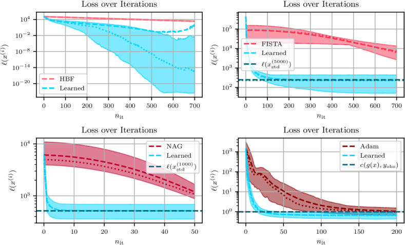
Therefore, in the second part of this work, we develop a concrete algorithmic realization, which allows for learning an optimization algorithm and evaluating the corresponding theoretical guarantee. This involves several design choices and tricks that have not been used before and which are of interest in their own right. Furthermore, as empirical evaluation of our claims, we conduct four practically relevant experiments, all dealing with very different classes of functions, thereby demonstrating the wide applicability and strong practical performance of our approach. Examples are shown in Figure 1. Each subplot compares the performance of the learned algorithm to that of a standard algorithm on different problems: a smooth and strongly convex quadratic toy problem (upper left), a high-dimensional, smooth and convex image processing problem (upper right), a non-smooth and convex LASSO problem (lower left), and a non-smooth and non-convex problem of training a neural network (lower right). Since the learned algorithm is clearly superior in each case, this provides a possible answer to the question about how to train optimization algorithms. Taken together, we provide a complete framework to train optimization algorithms with theoretical guarantees that are (in a certain sense) provably faster than their worst-case optimal counterparts. With this, we get closer to the ideal case of wide applicability, strong practical performance and sufficient theoretical guarantees. In particular, this work is a far reaching extension of our conference paper (Sucker and Ochs, 2023) by extending and clarifying the theoretical results in Sections 3, and by the algorithmic realization together with its evaluation in Sections 5 and 6, which additionally includes a probabilistic constraining procedure for sampling algorithms in Sections 5.2.
1.1 Related Work
The literature on both learning-to-optimize and the PAC-Bayes learning approach is vast. Hence, the discussion of learning-to-optimize will mainly focus on learning procedures for optimization algorithms and on approaches that provide some theoretical guarantees. Especially, this excludes many model-free approaches, which replace the whole update step with a learnable mapping such as a neural network. Chen et al. (2021) provide a good overview about the variety of approaches in learning-to-optimize, and good introductory references for the PAC-Bayesian approach are given by Guedj (2019) and Alquier (2021).
Broader Context of Learning-to-Optimize.
Solving optimization problems is an integral part of machine learning. Thus, learning-to-optimize has significant overlap with the areas of meta-learning (or “learning-to-learn”) and AutoML. The first one is a subset of learning-to-optimize, as, while learning-to-optimize applies to general optimization problems, meta-learning is mostly concerned with determining parameters of machine learning models, that is, minimizing a training loss (Vilalta and Drissi, 2002; Hospedales et al., 2021). AutoML, however, more broadly refers to automating all steps necessary to create a machine learning application, which thus also involves the choice of an optimization algorithm and its hyperparameters (Yao et al., 2018; Hutter et al., 2019; He et al., 2021). Hence, most relevant for this work is model selection.
Learning-to-Optimize with Guarantees.
Chen et al. (2021) point out that learned optimization methods may lack theoretical guarantees for the sake of convergence speed. That being said, there are applications where a convergence guarantee is of highest priority. To underline this, Moeller et al. (2019) provide an example where a purely learning-based approach fails to reconstruct the crucial details in a medical image. Also, they prove convergence of their method by restricting the output to descent directions, for which mathematical guarantees exist. The basic idea is to trace the learned object back to, or constrain it to, a mathematical object with convergence guarantees. Similarly, Sreehari et al. (2016) provide sufficient conditions under which the learned mapping is a proximal mapping. Related schemes, under different assumptions and guarantees, are given by Chan et al. (2016), Teodoro et al. (2017), Tirer and Giryes (2018), Buzzard et al. (2018), Ryu et al. (2019), Sun et al. (2019), Terris et al. (2021) and Cohen et al. (2021). A major advantage of these methods is the fact that the number of iterations is not restricted a priori. However, a major drawback is their restriction to specific algorithms and problems. Another approach, which limits the number of iterations, yet in principle can be applied to every iterative optimization algorithm, is unrolling, pioneered by Gregor and LeCun (2010). Xin et al. (2016) study the IHT algorithm and show that it is, under some assumptions, able to achieve a linear convergence rate. Likewise, Chen et al. (2018) establish a linear convergence rate for the unrolled ISTA. However, a difficulty in the theoretical analysis of unrolled algorithms is actually the notion of convergence itself, such that one rather has to consider the generalization performance. Only few works have addressed this: Either directly by means of Rademacher complexity (Chen et al., 2020b), or indirectly in form of a stability analysis (Kobler et al., 2020), as algorithmic stability is linked to generalization (Bousquet and Elisseeff, 2000, 2002; Shalev-Shwartz et al., 2010). We consider a mixture of the iterative approach and the unrolling approach: The theoretical analysis corresponds to the approach of unrolling, that is, a fixed number of iterations, and the resulting PAC-Bayesian generalization bound applies to this particular number osubsubsectionf iterations only. However, in our implementation and experiments, we stay more closely to the iterative approach of learning an update step that can be applied for an arbitrary number of iterations. Further, while the resulting algorithms do include neural networks in their update step, the construction is closely related to the model-based approach, as it is inspired by analytical algorithms.
Typical Problems and Tricks in Learning-to-Optimize.
The literature contains a vast amount of approaches, tricks and problems about learning procedures for optimization algorithms. We only touch briefly upon the ones that are most relevant for the present work:
Besides the actual optimizer, a typical design choice is that of the loss function. Here, either the final loss or a weighted sum of the losses incurred along the iterations is typically being used (Chen et al., 2021). This extends to choices about the computational graph, as one has to decide which gradients are computed during training. An assumption already made by Andrychowicz et al. (2016) and widely adopted thereafter, is to neglect higher-order derivatives. Importantly, if the theoretical analysis is coherent with the computational graph, one is allowed to do whatever works here.
A major problem of many learned optimization algorithms, especially the ones based on recurrent neural networks, is their restriction to a certain number of iterations, that is, they cannot be trained for an arbitrary number of iterations due to instabilities, such as vanishing or exploding gradients, and memory bottlenecks. Further, often they do not generalize well to more iterations (Andrychowicz et al., 2016; Chen et al., 2017; Lv et al., 2017; Chen et al., 2021). A typical way to mitigate this problem is to split the whole trajectory into smaller parts, for which the vanishing/exploding gradient phenomenon does not occur, which effectively also solves the memory problem. However, this often does not lead to fully satisfactory results either, such that other approaches have been proposed: Lv et al. (2017) introduce random scaling of the coordinates and the addition of a convex function to the objective. Metz et al. (2019) propose not to model the recurrent nature of optimization algorithms directly, and therefore to replace the recurrent neural network with a multilayer perceptron, to “smooth” the loss, and to dynamically use two unbiased gradient estimators instead of one. Doing so they manage to train algorithms that are faster in wall-clock time than standard ones like Adam. Wichrowska et al. (2017) introduce a hierarchical RNN architecture consisting of three RNNs, and additionally draw the number of unrollings and the unrolling length from a heavy-tailed exponential distribution. While achieving the needed generalization, this approach is computationally costly and does not achieve the same wall-clock time as simple optimization algorithms. Chen et al. (2020a) consider improved training techniques in general, and they introduce a progressive scheme that gradually increases the unrolling length, and an imitation learning approach by learning from analytic optimizers first. We will introduce a new loss function for training optimization algorithms, motivated by an intuitive theoretical argument. To our best knowledge, this loss function is new. Here, we will typically also ignore higher-order derivatives in the computational graph, as the algorithms performance is analyzed independently of this step in the learning procedure. Further, we found that a combination of many of the above mentioned approaches works well: 1) We use a single learned update based on MLPs and analytic algorithms instead of an RNN. 2) We split the trajectory into subtrajectories and randomize its total length, however, in a different and new way, again motivated by theoretical considerations. 3) We start the learning procedure with imitation learning to find an initialization that performs similar to analytic algorithms.
PAC-Bounds through Change-of-Measure.
The PAC-Bayesian framework allows for giving high probability bounds on the risk, either as an oracle or as an empirical bound. The key ingredients are so-called change-of-measure inequalities. The choice of such an inequality strongly influences the corresponding bound. The one used most often is based on a variational representation of the Kullback–Leibler divergence due to Donsker and Varadhan (1975), employed, for example, by Catoni (2004, 2007). Yet, not all bounds are based on a variational representation, that is, holding uniformly over all posterior distributions (Rivasplata et al., 2020). However, most bounds involve the Kullback–Leibler divergence as measure of proximity, for example, those by McAllester (2003a, b), Seeger (2002), Langford and Shawe-Taylor (2002), or the general PAC-Bayes bound of Germain et al. (2009). More recently, other divergences have been used: Honorio and Jaakkola (2014) prove an inequality for the -divergence, which is also used by London (2017). Bégin et al. (2016) and Alquier and Guedj (2018) use the Renyi-divergence (-divergence). Ohnishi and Honorio (2021) propose several PAC-bounds based on general f-divergences, which include the Kullback–Leibler-, - and -divergences. Even more recently, Amit et al. (2022) propose to replace the Kullback-Leibler divergence by so-called “integral probability metrics”, which encompass, for example, the Wasserstein distance that obeys many favorable properties and also captures the geometry of the underlying space (see Villani et al., 2009). Motivated by this, Haddouche and Guedj (2023) also investigate PAC-Bayesian generalization bounds for the Wasserstein distance and their interplay with the output of optimization algorithms. A major advantage of using the Wasserstein distances instead of the Kullback-Leibler divergence is the fact that it does not constrain the support of the distribution a-priori through the choice of the prior. On the other hand, it demands assumptions on the loss function, which are not necessarily satisfied in learning-to-optimize. We give a general PAC-Bayesian theorem based on exponential families. Here, the role of prior, posterior, divergence and data dependence will be given naturally. Moreover, this approach allows us to implement a more abstract learning framework that can be applied to a wide variety of algorithms.
Boundedness of the Loss Function.
A major drawback of many of the existing PAC-Bayes bounds is the assumption of a bounded loss-function. However, this assumption is mainly there to apply some exponential moment inequality like the Hoeffding- or Bernstein-inequality (Rivasplata et al., 2020; Alquier, 2021). Several ways have been developed to solve this problem: Germain et al. (2009) explicitly include the exponential moment in the bound, Alquier et al. (2016) use so-called Hoeffding- and Bernstein-assumptions, Catoni (2004) restricts to the sub-Gaussian or sub-Gamma case. Another possibility to ensure the generalization or exponential moment bounds is to use properties of the algorithm in question. London (2017) uses algorithmic stability to provide PAC-Bayes bounds for SGD. We consider suitable properties of optimization algorithms aside from algorithmic stability to ensure the exponential moment bounds. To the best of our knowledge, this is new.
Minimization of the PAC-Bound.
The PAC-bound relates the true risk to other terms such as the empirical risk. Yet, it does not directly say anything about the absolute numbers. Thus, in learning procedures based on the PAC-Bayesian theory one typically aims to minimize this bound: Langford and Caruana (2001) compute non-vacuous numerical generalization bounds through a combination of PAC-bounds with a sensitivity analysis. Dziugaite and Roy (2017) extend this by minimizing the PAC-bound directly. Pérez-Ortiz et al. (2021) also consider learning as minimization of the PAC-Bayes bound and provide tight generalization bounds. Thiemann et al. (2017) are able to solve the minimization problem resulting from their PAC-bound by alternating minimization. Further, they provide sufficient conditions under which the resulting minimization problem is quasi-convex. We also follow this approach and consider learning as minimization of the PAC-Bayesian upper-bound, however, applied to the context of learning-to-optimize.
Choice of the Prior.
A common difficulty in learning with PAC-Bayesian bounds is the choice of the prior distribution, as it heavily influences the performance of the learned models and the generalization bound (Catoni, 2004; Dziugaite et al., 2021; Pérez-Ortiz et al., 2021). In part, and especially for the Kullback-Leibler divergence, this is due to the fact that the divergence term can dominate the bound, keeping the posterior close to the prior. This leads to the idea of choosing a data- or distribution-dependent prior (Seeger, 2002; Parrado-Hernández et al., 2012; Lever et al., 2013; Dziugaite and Roy, 2018; Pérez-Ortiz et al., 2021), which, by using an independent subset of the data set, gets optimized to yield a good performance. The choice of the prior distribution is crucial for the performance of our learned algorithms. Thus, we use a data-dependent prior. Further, we show how the prior is essential in preserving crucial properties during learning. It is key to control the trade-off between convergence guarantee and convergence speed. Based on these insights, a major part of our algorithmic realization is concerned with constructing such a prior distribution.
More Generalization Bounds.
There are many areas of machine learning research that study generalization bounds and have not been discussed here. Importantly, the vast field of “stochastic optimization” (SO) provides generalization bounds for specific algorithms. The main differences to our setting are the learning approach and the assumptions made:
-
•
In most of the cases, the concrete algorithms studied in SO generate a single point estimate by either minimizing the (regularized) empirical risk functional over a possibly large data set, or by repeatedly updating the point estimate based on a newly drawn (small) batch of samples. Then, one studies the properties of this point in terms of the stationarity measure of the true risk functional (Bottou et al., 2018; Davis and Drusvyatskiy, 2022; Bianchi et al., 2022). In our case, as we consider the PAC-Bayesian learning approach, the final object to be studied is a distribution over hyperparameters.
-
•
As the setting in SO is more explicit, more assumptions have to be made. Typical assumptions are (weak) convexity (Shalev-Shwartz et al., 2009; Davis and Drusvyatskiy, 2019), bounded gradients (Défossez et al., 2022), bounded noise (Davis and Drusvyatskiy, 2022), or smoothness (Kavis et al., 2022). Since we consider an abstract optimization algorithm, and the problem of finding a distribution over its hyperparameters, all of these assumptions cannot be made without severely limiting the applicability of our results.
We provide a principled way to learn a distribution over general hyperparameters of an abstract algorithm under weak assumptions and go explicitly beyond analytically tractable quantities. Therefore, the methodology is independent of the chosen implementation.
2 Problem Setup & Assumptions
In this section we establish the notation, formalize the setting, and state the main assumptions that are used throughout the remainder of the text.
Notation.
We will endow every topological space with the corresponding Borel--algebra , and, given a product space of two measurable spaces and , we endow it with the product--algebra . To denote the product space of a larger number of spaces , we will use as the shorthand for and for the product--algebra. Further, if , we also use . If we are given a multivariate function , then denotes the function with fixed element . Similarly, for a set we denote the section of for fixed by . In general, generic sets are denoted in the typewriter font, for example , and denotes the function that is equal to one for and zero else, while denotes the function that is equal to zero for and else.111We omit the name here, as both and are called “indicator function”. The former in probability theory, the latter in optimization. For a measure on a measurable space , and a measurable function on , denotes the integral of w.r.t. , while, if , denotes the measure given by , that is, and . Hence, by definition, the measure is absolutely continuous w.r.t. , written as , with being the corresponding density. Here, the set of all measures on a measurable space will be denoted by , and the set of all probability measures that are absolutely continuous w.r.t. are denoted by . Here, the Kullback-Leibler divergence between two measures and is defined as
If is actually the specific probability measure of the underlying probability space , the corresponding expectation is denoted by . Random variables, that is, measurable functions on , are written in Fraktur-font, for example . Given two random variables, say and , integration of a function on w.r.t. the induced probability measure is specified by the subscript , that is:
If we are given a regular version of the conditional distribution of , given , denoted by , their joint distribution can be disintegrated into the product of the marginal and the probability kernel , which allows us to use the notation:
Note that, in this case, naively changing the order of integration is not allowed. However, if and are independent, their joint distribution is given by the product measure for which Fubini’s theorem is applicable, and the iterated integration is clarified by the corresponding subscripts :
Furthermore, we will denote the extended real numbers by . Since it holds that , any -measurable function can be identified with a -measurable function (Klenke, 2013, p. 38, Corollary 1.87). Finally, our theoretical results will rely on the notions of probability kernels, Polish spaces, and exponential families, whose definitions are recalled in Appendix A.
2.1 Main Assumptions and Definitions
We assume that, inside the class of functions that is encoded analytically in the model, we are given a distribution over loss-functions with a specific structure, which is modelled by a random variable:
Assumption 2.1
We are given a probability space and, for some fixed , we are given random variables , where is a Polish space. Further, we are given a non-negative and measurable loss-function .
Remark 2.2
The assumption of a Polish space is not restrictive, yet suffices to ensure the existence of regular versions of the conditional probability distribution, that is, for the disintegration of a joint distribution into a marginal and a corresponding probability kernel (see Kallenberg, 2021, Thm. 8.5).
Then, ideally, we would like to find a solution to each realization of the random objective:
| Find , s.t. | (1) |
However, we will only solve a relaxed version of (1) and provide generalization bounds for the average performance. Implicitly, we assume that we are given several realizations with similar structure, as . This is close to the “standard” learning problem, where an algorithm gets trained on a data set and then applied to unseen data. For this, we need to have a data set:
Definition 2.3
The measurable function is called a data set. Here, is called the data-space. If the induced distribution factorizes into the product of the marginals, that is, if , it is called independent and if, additionally, it satisfies , it is called i.i.d.
PAC-Bayesian generalization bounds involve a so-called posterior distribution, which usually is a “data-dependent distribution”. Often, this term is left unspecified. Yet, as also pointed out by Rivasplata et al. (2020), this is an instance of a probability kernel (also called a “stochastic”- or “Markov kernel”). Another commonly used name is “regular conditional probability”, following the definition of a regular conditional distribution through probability kernels (Catoni, 2004; Alquier, 2008). In our opinion, the notion of a probability kernel is the least ambiguous one, leading to the following definition:
Definition 2.4
Let be a data set with data-space , and let be a measurable space. A probability kernel from to is called a data-dependent distribution on .
For solving problem (1), for every realization of , we apply an optimization algorithm to . For this, we consider a similar setting as London (2017), that is, randomized algorithms are considered as deterministic algorithms with randomized hyperparameters:
Definition 2.5
Let be a Polish space and . A measurable function
is called a parametric algorithm and is called the hyperparameter space of . is the space of the optimization variable, the space of the parameters of the problem instance, and the space of the hyperparameters of the algorithm.
Remark 2.6
corresponds to the whole algorithm, that is, its output is the final iterate of the optimization procedure, which has to be stopped after some iteration , and could be contrasted with the notion of an estimator in statistics. However, one can also model a single update-step, and recover as k-fold concatenation of this update-step.
Here, learning refers to finding a distribution on based on its performance on a data set . In the PAC-Bayesian approach to learning and generalization, one needs a reference distribution, which can (and should) encode prior knowledge about suitable choices of hyperparameters, called the prior:
Assumption 2.7
We are given a parametric optimization algorithm with Polish hyperparameter space , and a (prior) distribution on that is induced by a random variable , which is independent of the data set and . Further, the initialization is given and fixed.
Notation 2.8
We will refer to the random variable as the parameters of the loss-function and to as the hyperparameters of the algorithm . Further, to simplify the notation, we also use the short-hand . Furthermore, if not needed explicitly, and will not be mentioned anymore in the following.
Now, we define the risk of a randomized parametric optimization algorithm as usual:
Definition 2.9
The following theory is based on exponential families (see Definition A.4). This is a class of distributions on some space , which is mainly build upon three parts: a function on some index set , a function on , and a distribution on . Since we want to have a distribution over hyperparameters , we will choose . However, then, the exponential family is not data-dependent. Therefore, we will define data-dependent exponential families by extending the domain of from to .
Definition 2.10
Let be a data set with data-space , and let be a non-empty index set. A family of probability measures on a measurable space is called an data-dependent exponential family (in and ), if there is a dominating probability measure , that is, , functions , , and measurable functions , , such that we have for every , , that is, , .
Remark 2.11
If describes a lower-dimensional manifold in , is called a curved exponential family (Efron, 1975), whose properties might differ from the ones for linear exponential families (), for example, convexity of the map .
We introduce data-dependency through , since it strongly affects the shape of the distribution and, contrary to , is defined on the underlying space . Since we want to learn a distribution over hyperparameters , we make the following assumption:
Assumption 2.12
On the hyperparameter space , we are given a data-dependent exponential family in and with dominating probability measure , such that the map is non-trivial and integrable w.r.t. for every , , that is, .
Remark 2.13
-
(i)
In PAC-Bayes, the dominating measure is usually referred to as prior and every distribution is referred to as a posterior. This deviates from the standard definitions of prior and posterior in Bayesian statistics.
-
(ii)
The integrability assumption is slightly restrictive, as it affects the choice of and . However, in Section 4 we will construct and such that this holds anyway.
The last integral in Assumption 2.12 will be of great interest in the following. Here, we will use a similar notation as in Barndorff–Nielsen (2014) and denote
| (2) |
or for short, . With this notation, it holds that . Through this, as shown in Lemma B.1, every member of the data-dependent exponential family is indeed a data-dependent distribution on in the sense of Definition 2.4. Finally, we will restrict the space to a compact set. This is needed to get a uniform bound in , and such ideas appeared in the literature (see Langford and Caruana, 2001; Catoni, 2007; Alquier, 2021).
Assumption 2.14
is a compact set with finite covering , that is, , such that there is a constant , which, for every , allows for the bound .
Remark 2.15
The existence of a general finite covering for is a consequence of the compactness. However, the existence of the constant is non-trivial. It does hold, for example, if is a finite set (, ), or, if is a compact metric space and is Lipschitz-continuous in (uniformly in ) with Lipschitz constant L, such that , where the diameter of a set is given by .
3 General PAC-Bayesian Theorem
In this section we prove the following general PAC-Bayesian bound for data-dependent exponential families, which then can be specialized into a generalization bound of the learned parametric optimization algorithm . It is based on the following two lemmas, whose proofs can be found in Appendix C and D, respectively. The first lemma is a form of the Donsker–Varadhan variational formulation and yields uniformity in the distributions :
Lemma 3.1
Similarly, the second lemma yields uniformity in . For this, we need to be able to cover , and to control for every , as specified in Assumption 2.14.
Lemma 3.2
Suppose that Assumption 2.14 holds and assume that for all and . Then .
Taken together, these two lemmas allow us to state the PAC-Bayesian theorem in its general form:
Theorem 3.3
Proof For every , is a non-negative random variable, and is monotonically increasing. Thus, Markov’s inequality yields for :
Thus, , because is equivalent to . Hence, Lemma 3.2 is applicable and gives:
Using Lemma 3.1 gives:
Simply rearranging and reformulating yields the result.
Remark 3.4
-
(i)
Note that the statement is still true for a data-dependent prior : Denoting the additional data set by , one needs to assume that . Also Lemma 3.1 still applies “pointwise” (with the appropriate notational adjustments). Intuitively, this is due to the fact that the PAC-bound is a statement about relative, and not absolute values.
-
(ii)
In Section 4 we provide sufficient conditions s.t. holds for all .
-
(iii)
bears the intrinsic dimension of and thus, in full generality, might be large. For our generalization bound, however, it has only a minor influence, since there , and the the empirical risk is typically much larger.
For the rest of the paper, we will have , such that . The following corollary, whose proof is given in Appendix E, shows how to transform Theorem 3.3 into a high-probability bound on the risk.
Corollary 3.5 (PAC-Bayesian Generalization Bound)
Denote the coordinates of and by and . If and , the following are equivalent for any , , :
-
(i)
,
-
(ii)
In particular, if Theorem 3.3 applies, we can replace (i) with (ii).
4 Learning-to-Optimize with Guarantees
Here, we consider properties of optimization algorithms, that assert the necessary condition for all to employ the PAC-Bayesian bound from Section 3.
4.1 Guaranteed Convergence
In the next theorem, the additional assumption on is sufficient to ensure the assumptions of Theorem 3.3. Essentially, it requires the loss of the algorithm’s output to be bounded. Yet, as shown in Section 4.2, it is too restrictive to learn hyperparameters that allow for a significant acceleration compared to the standard choices from a worst-case analysis.
Theorem 4.1
Suppose that and satisfy Assumption 2.1, and suppose that satisfies Assumption 2.7. Further, assume that there is a constant and a measurable function , such that for every it holds that -a.s. Furthermore, let be a corresponding i.i.d. data set of size . Finally, assume that , and define and through:
Then it holds that for all .
Proof Since and are independent, their joint distribution is given by the product measure . Further, , such that Fubini’s theorem is applicable and allows to do the integration iteratively, that is:
Hence, first consider the inner integral for a fixed . Then, by definition and the i.i.d. assumption one gets:
The loss-function is non-negative and ,by assumption, can be bounded -a.s. Thus, for every , is a non-negative random variable with finite second-moment, as . Thus, by Lemma B.2, the boundedness assumption on , and the monotonicity of the exponential function, one gets the bound:
Therefore we have the following bound:
This can be rearranged into , as the right-hand side does not depend on . Since and are independent, and was arbitrary, this inequality does hold -a.s. Therefore, one directly gets the bound . Now, again by Fubini’s theorem, one can also switch the order of integration to get:
Inserting the definition of and gives . Here, the inner term is the same as
. Hence, this is the same as .
Remark 4.2
The argument still works for a data-dependent prior, if the corresponding data sets and are independent: While interchanging the integration w.r.t. and is not allowed, an interchange w.r.t. and is still valid (under the integral), that is, for a function it would hold , and the inner term is in any case. The premise here is that the boundedness assumption on holds.
4.2 Conditioning on Convergence
Most of the time, the previous approach learns hyperparameters that ensure convergence, since the boundedness assumption on implicitly requires weak theoretical worst-case estimates almost surely. If, for example, the considered class of functions is that of general quadratic functions, the convergence behaviour is accurately represented by analytic quantities from a worst-case analysis. Thereby, the boundedness prevents “aggressive” step-size parameters that lie outside the worst-case convergence regime, as they would lead to a diverging behaviour, which increases the incurred empirical risk dramatically. Thus, to motivate the upcoming discussion, consider the following thought-experiment:
Example 4.3
Consider and assume that the chosen algorithm is gradient descent, that is . For a given , the optimal step-size is , which gives convergence in one step. However, if is given by samples from the distribution , a worst-case analysis would suggest to take . In this case, we would have an algorithm that converges in a single step for 1% of the problem instances, while having a linear convergence rate of for the other 99%. Another choice is to take , which leads to an algorithm that does converge in a single step for 99% of the problem instances, but diverges in 1% of the cases. By restricting to the 99% of the cases where convergence does occur, the overall difference in speed is drastic.
Hence, in this section, a different approach is taken: We actually allow for divergence, if it only occurs in rare cases with a controllable probability, that is, “almost surely” is relaxed to “with a sufficiently large probability”. Essentially, we only consider the loss for all those hyperparameters, where the loss is bounded by a certain constant, as well as the probability for that to occur. Then, in Section 4.2.1, we develop a technique that allows the user to actually control this probability. Clearly, a stronger guarantee trades for convergence speed.
Definition 4.4
Given a measurable function , the (parametric) sublevel set is defined as . The sections of for fixed will be denoted by .
Remark 4.5
The concrete choice of will influence the PAC-Bayesian bound. Again, for proving the result, the essential property is that the loss after applying can be bounded.
In Lemma B.3 we show that is indeed a measurable set. This is not obvious, as the loss function and the algorithm are composed in a non-standard way. This result further implies that the sections are measurable, too. Since and are Polish spaces, the product is again Polish. Hence, there exists a regular version of the conditional probability of , given , that is, a kernel . By Witting (2013, Thm. 1.122, p.124), this determines a regular version of the conditional probability of , given , through . Here, for any measurable function for which exists, it holds -a.s.:
| (3) |
Thus, we get -a.s. the equality . In particular, this applies to the sublevel set , and the map is measurable.
Definition 4.6
Let be a parametric sublevel set. Define the sublevel probability as the measurable function .
Lemma 4.7
Suppose Assumption 2.7 holds, and let for every . Then we have -a.s.:
-
(i)
,
-
(ii)
.
Proof
By (3) and the independence of and , we have -a.s., which shows the first equality of (ii). Since , the elementary conditional expectation is defined as . Again by independence we have -a.s. the equality , which shows (i) and the second equality of (ii).
This construction allows us to give a more fine-grained analysis of the algorithm, as it allows to trade the boundedness assumption for the sublevel probability. This basically extends a worst-case analysis, which would correspond to an uniform upper bound. Motivated by Lemma 4.7, to actually analyze the algorithm in this setting, we define the sublevel risk and its empirical counterpart as the expect loss conditioned on the sublevel set:
Definition 4.8
Let be a parametric sublevel set. Then the sublevel risk is defined as the conditional expectation of the loss given :
Given a data set , the empirical sublevel risk is defined as .
The following theorem is a direct generalization of Theorem 4.1. Especially, note that the additional assumption on is not needed anymore.
Theorem 4.9
Proof The proof is very similar to the proof of Theorem 4.1 and basically uses the same reasoning. Let . Since and are independent, and , one gets from Fubini’s theorem:
Thus, first consider a fixed with . Then, by definition and the i.i.d. assumption, it holds that:
is non-negative, and by definition of the parametric sublevel set has a finite second-moment, that is . Hence, by Lemma B.2 we have the inequality . Thus:
This can be rearranged into , since the right-hand side is independent of . As this holds for any with , which in turn does hold -a.s., we get . Changing the order of integration with Fubini’s theorem, we get:
Using the definition of and , this is the same as
The inner term can be rewritten as . Hence, in total we get .
Remark 4.10
4.2.1 Implementing the Non-divergence – Speed Trade-Off
In Section 4.2, care has to be taken in the choice of the prior : Just minimizing the upper bound as much as possible can lead to a neglection of a high sublevel probability, that is, the algorithm is especially fast on a small subset of the parameters, while it diverges for the rest, because the term might not compensate for the smaller sublevel risk. Thus, if a certain sublevel probability has to be ensured, one has to enforce it. We propose to use absolute continuity:
Lemma 4.11
Let and assume that a.s. Then, for every we have .
Proof
Since , we have . Thus, the result follows by definition of absolute continuity.
Though the proof is trivial, this lemma has a very important consequence, which we want to stress: If one can guarantee that a required property is satisfied for the prior, it will be preserved during the PAC-Bayesian learning process, that is, if the prior only puts mass on hyperparameters that ensure a certain sublevel probability, the posterior will do the same. We will enforce this constraint in the learning procedure, which is discussed next.
5 Learning Procedure
This section deals with the learning procedure, that is, how the abstract framework discussed in Sections 3 and 4 is actually implemented. Hence, this is also the beginning of the second part of the paper, which is of a more practical kind and less theoretical. The resulting learning procedure is visualized in Figure 2 and consists of four steps:
-
(i)
Find an initialization that is trainable in a stable way: This is due to the fact that one might include, for example, a neural network in the update step of , which, if initialized randomly, might predict points at the very beginning, that are so far off that one encounters numerical instabilities. Hence, we first train the algorithm to “follow” another algorithm , just for the purpose of non-divergence.
-
(ii)
Locate the prior by finding a point that satisfies the constraint in Subsection 4.2 and yields a good performance. For this, we perform a constrained version of stochastic empirical risk minimization with a new, specifically designed loss function.
-
(iii)
Starting from , construct the prior distribution by running a constrained version of a sampling algorithm.
-
(iv)
Compute the posterior distribution by finding the optimal and performing the reweighting with the closed form for .
Hence, first, in Subsection 5.1 we will identify the optimal posterior in the abstract setting. Second, in Section 5.2, we realize the constraining procedure, which allows to keep an optimization or sampling procedure inside an abstractly defined set . Lastly, we put things together in Section 5.3 and finalize the learning procedure by concretizing each single step: Section 5.3.1 deals with the pre-computation phase in (i), Section 5.3.2 deals with the initialization in (ii), Section 5.3.3 provides the concrete choice of prior distribution in (iii), and Section 5.3.4 finally yields the posterior distribution in (iv).
5.1 Minimization of the PAC-Bound
Because learning is phrased as minimizing the PAC-Bayesian upper-bound, this is the first thing to do. Hence, in this subsection we consider , and item from Corollary 3.5. We seek for and that minimize the upper-bound in Corollary 3.5 , that is, we want to solve:
By factoring out again, this is actually the same as:
where . Since is a constant, Lemma 3.1 shows that the term inside the brackets is given by , where corresponds to the exponential family built upon and (with ). Furthermore, it shows that the (in this sense) optimal posterior distribution is given by the corresponding member of the data-dependent exponential family , usually called the Gibbs posterior (Alquier, 2021). By denoting , one is left with solving the following problem:
| (4) |
which for is one-dimensional. Based on Theorem 4.1 and Theorem 4.9, we have to restrict to , such that the solution to (4) can be seen as an approximation to the global minimum . For the latter one, one can show that the solution set lies in a compact interval , with , since as or . Under our assumptions, is continuously differentiable. Hence, since is compact, is Lipschitz-continuous on and the minimum in (4) is attained. For a finite , the optimization reduces to grid search. For , we employ grid search as initialization for gradient-based optimization. However, we still might get stuck in a (close to optimal) local minimum. The computational bottleneck is given by evaluating . In Sections 5.3.3 and 5.3.4 we will ensure that this is cheap.
5.2 Sampling under Probabilistic Constraints
In this section, we describe a methodology that allows for sampling from a distribution that is probabilistically constrained in the following sense: We are given two independent random variables , taking values in the Polish spaces and , with joint and marginal distributions , and , respectively. Further, we consider a measurable set , and we want to generate samples , such that the probability of lying in , given , takes values in a certain interval:
By independence of and , this is -almost surely the same as , and we will use the later formulation from now on. While having an abstract description of , we do not have any explicit information about its geometrical or topological properties, let alone access to a distance or a projection onto it, and the marginal can only be accessed via samples , . However, since we are able to evaluate, for every and , whether , this allows to define a function , given by:
Then is indeed a measurable function, taking values in . Thus, for with , we can define a measurable set , which yields a new measure on by restricting to , that is, for a measurable set it holds:
Therefore, as stated before, we have the following goal:
| Goal: Sample from , that is, get , such that . |
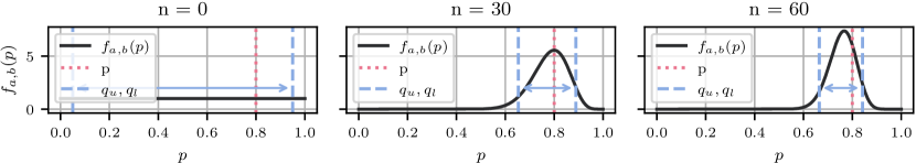
This construction is depicted in Figure 3: The left figure visualizes the sections of the set , while the right figure shows the corresponding construction of the support of . Here, we assume that the imposed constraint is realizable.
Assumption 5.1
The measure has a non-empty support.
Remark 5.2
Assumption 5.1 includes two things: (i) There have to be points (hyperparameters) for which the property in does hold, that is, it has to be realizable. (ii) The support of (prior) has to have a non-empty intersection with this region.
Example 5.3
5.2.1 Incorporation into a Sampling Procedure
By definition it holds that on . Hence, the only distinction between samples from and samples from is the restriction to the set . Therefore, since many sampling algorithms sample from unnormalized measures anyways, it suffices to be able to sample from , if the restriction to can be satisfied in other ways. Thus, we have to integrate this constraint into a sampling procedure for . Because we do not have any geometrical or topological information about the set , we have to resort to statistical information: We have access to i.i.d. samples , and, for a given , we are able to evaluate the i.i.d. Bernoulli-distributed random variables , . These have the parameter . Thus, by estimating with an estimator , we can approximate the constraint with :
Given a sample , we resort to a simple accept-reject mechanism as in Metropolis-Hastings-type algorithms (Robert and Casella, 2004), to decide whether , that is, whether can actually be regarded as a sample from .
Remark 5.4
We believe that this is the only reasonable choice here, which keeps an iterative algorithm inside . However, it does not provide a way into , let alone .
We estimate in a Bayesian way, as it allows us to balance accuracy against computational complexity through uncertainty-quantification, which we use as a stopping criterion: We place a Beta-prior over the interval . As we do not have prior knowledge, and the map can be discontinuous222Consider learning the step-size parameter for gradient descent on quadratic functions with largest eigenvalue : The algorithm converges for () and diverges for () ., we use a noninformative prior (Berger, 1985, Ch. 3.3), that is, . Since the Beta distribution is the conjugate prior for the Bernoulli distribution (Berger, 1985, p.130), that is, the posterior is again a Beta-distribution, after observing a sample , the parameters get updated as:
Hence, we can perform the estimation iteratively: We only draw a new sample as long as , where denotes the quantile-function of the distribution , and are parameters that specify the accuracy of the estimation. Finally, one can use the posterior mean or posterior mode (provided ) as point estimate . This procedure is summarized in Algorithm 1 and depicted in Figure 4.
Remark 5.5
By adjusting or , one can balance between accuracy and computational complexity. Yet, the number of iterations needed also depends crucially on the true probability: For or , the uncertainty decreases significantly faster than for .
5.2.2 Broader Context
Different, yet conceptually similar ideas have appeared in the context of cutting the computational cost of Bayesian Markov Chain Monte Carlo algorithms through subsampling: Korattikara et al. (2014) introduce sequential hypothesis tests to reach the binary accept-reject decision in the Metropolis-Hastings algorithm on subsamples of the data set. Similarly, Bardenet et al. (2014) estimate the accept-reject step on a random subset of the data, in a way that guarantees to coincide with the true accept-reject step with a user-specified probability. Maclaurin and Adams (2014) introduce an auxiliary binary variable , which allows to query only a subset of the data for the computation of the exact likelihood. And Quiroz et al. (2018) use a subsampling and bias-correction strategy to speed-up the sampling procedure. Here, Bardenet et al. (2017) provides a summary and discussion of different approximations and their biases (and errors). We leave the corresponding analysis for our proposed approximation to future work.
5.2.3 Choice of the Sampling Procedure
Often, the hyperparameters of the learned algorithm are high-dimensional. Thus, we resort to using stochastic gradient Langevin dynamics (Welling and Teh, 2011) as the underlying sampling algorithm, which gets constrained to the set by use of the previously described procedure. This is summarized in Algorithm 2. However, if it fits the application, other sampling algorithms can be used, too. The computational overhead of the additional estimation depends on the cost of evaluating . In our case it is rather expensive, as every sample requires to run the algorithm . However, this is to be expected, as the “prediction” of an optimization algorithm corresponds to approximating the solution of a minimization problem.
Remark 5.6
Algorithm 2 requires to start in the set . If such a point is not known, one can still run the algorithm and just “start” the accept-reject mechanism as soon as one has found a point . However, it is not guaranteed that such a point will actually be found.
5.3 Putting Things Together
In the abstract learning procedure described in Sections 3 and 4 everything relies on the existence of a prior distribution that a) gives a good performance of the algorithm in terms of a small risk, and b) ensures the user-specified sublevel probability. Both a) and b) have to be enforced through the construction of the prior , which is why often a data-dependent prior is used (Parrado-Hernández et al., 2012; Lever et al., 2013; Dziugaite and Roy, 2017, 2018; Dziugaite et al., 2021). Note that a) and b) are qualitatively different: a) asks for a certain location and concentration of , while b) puts hard constraints on its support, that is, it excludes many frequently used distributions with unconstrained support. Therefore, a significant part of the learning procedure deals with the construction of this prior only. Since the prior will be data-dependent, yet has to be independent of the data set that is used in the PAC-Bayesian learning procedure in Section 5.3.4, we have to split the data set into independent parts , , and , where and are used for the construction of the prior distribution, is used for the PAC-Bayesian learning step, and is the test set to evaluate the performance, that is, it is only needed for the experiments. Nevertheless, for notational simplicity, we will use the generic , implicitly assuming the above partitioning. As the data set is fixed now, it will be described by the corresponding realization of the random variable .
Remark 5.7
Through the choice of the sampling algorithm, the concrete learning procedure described here mainly applies to the case , . Nevertheless, the general methodology is still applicable to other Polish spaces, if this choice can be adjusted accordingly.
5.3.1 Finding a Trainable Initialization
To increase numerical stability, we start with “imitation learning” (Chen et al., 2020a), that is, the algorithm should “follow” another algorithm , for example, gradient descent. For this, we minimize the mean squared error between the iterates of the two algorithms: Given a starting point , an iteration number , and a parameter , denote the first iterates of by and the ones of by . Then, define the loss as the mean squared error over these iterations:
In each iteration, that is, each prediction of tuples , the parameters , and are randomized as described in Section 5.3.2. We postpone the discussion of this step, as it is an integral part of the learning step described there, while being less important here. We terminate the process as soon as the average loss over iterations reaches a certain level of accuracy , that is, as soon as . The choice of and depends on the problem at hand. Usually, rough estimates suffice (), as the purpose is to prevent divergence, and not actual imitation of . The procedure is summarized in Algorithm 3.
5.3.2 Locating the Prior
Empirically, the performance of the learned algorithm is significantly improved by the following two design choices, namely randomizing the trajectory length and using the ratio of successive losses. The motivation is to prevent overfitting and to learn a scale-independent contraction of the loss:
1) Ratio of Losses: Since the algorithm should achieve a small risk , yet minimizing is intractable, the canonical loss function to be minimized is . As might be high-dimensional, we resort to stochastic empirical risk minimization, that is, in each iteration the observed loss would be of the form . While this kind of loss was used extensively before, for learning-to-optimize it has a strong disadvantage: The overall outcome gets penalized only after the application of the whole algorithm, that is, after iterations of the update-step. Thus, it does not take the trajectory into account. Further, often it is hard to minimize and does not lead to the desired performance. To circumvent this, Andrychowicz et al. (2016) proposed to use the sum over the incurred losses, that is, to consider . Again, this formulation has a decisive flaw: Under most objectives, if the algorithm performs reasonably well, the loss at the beginning is several orders of magnitude larger than the loss at the end, that is, . Hence, mainly penalizes the loss at the beginning, leading to an algorithm that minimizes the loss very fast in early iterations, but slows down a lot in later iterations. This is due to being scale-sensitive. Additionally, the incurred loss might vary strongly with the initialization alone, thereby introducing ambiguity into the incurred losses. We propose to use the ratio of losses of successive iterates:
This has several advantages: First, the loss is not scale-sensitive anymore, such that it favours hyperparameters that yield a good performance in each iteration. Second, there is no ambiguity in the observed loss through the initialization, as the only criterion is a strong contraction of the loss (instead of a small loss). Intuitively, the algorithm gets trained to have a fast convergence rate. Third, the incurred losses do not vary too much, which empirically makes it easier to choose hyperparameters of the learning procedure. However, it also has a disadvantage: If the function values do indeed converge in a setting where the optimal loss is strictly greater than zero, this gets fully penalized, as then . For now, we do not know how to get rid off this problem (apart from just stopping the iterations in case of convergence) while keeping the advantages, yet we (successfully) combat it with a decreasing step-size during training.
2) Randomized Trajectory Length: Training with fixed initialization and fixed trajectory length , leads to overfitting, that is, applying at another starting point , or applying it for more than iterations typically leads to divergence. To get rid off this, we propose the following randomization: Given , set and .
-
0)
Sample a parameter uniformly at random from .
-
1)
Compute with and the loss , and update .
-
2)
Sample . If , set and go to step 1). If , set and go to step 0).
The random variable decides whether the algorithm gets restarted from with a new parameter , or if one continuous the current trajectory. To update , we use backpropagation and Adam. The choice ensures that the expected trajectory-length equals : Define . Then, is a geometrically distributed with expectation . Therefore, the actual length of the trajectory is (basically) a geometrically distributed random variable with .
Remark 5.8
-
(i)
Similarly to Andrychowicz et al. (2016), during training we omit the computation of second order derivatives. Additionally, and surprisingly, it usually suffices to consider single iterates, that is , where the iterates are treated independently in the computational graph. That amounts to learning an update step that is agnostic to the recurrent nature of the optimization algorithm and just learns to adapt to the local geometry of the loss function along the iterations.
-
(ii)
Splitting the trajectory into several parts has been used before, especially in model-free approaches based on recurrent neural networks (Andrychowicz et al., 2016; Chen et al., 2017; Metz et al., 2019), where the main motivation are training instabilities and memory bottlenecks. Similarly, randomizing the trajectory length did appear in Wichrowska et al. (2017). Yet, to our knowledge, our specific randomization is new, theoretically motivated, and solves the problem of generalizing to more iterations quite effectively.
Empirically, by using these design choices we are able to train in a way such that it performs equally well on several orders of magnitude of the loss function, and that it can be used for more iterations than it was actually trained for. The procedure is summarized in Algorithm 4 and consists of three steps:
-
1)
Given and , compute a new proposal by performing one step of Adam on , corresponding to iterations of .
-
2)
Check for the constraint by estimating it with Algorithm 1. If the constraint is satisfied (or one did not find any point inside the constraint so far), accept . Otherwise, reject it and sample a new problem instance .
-
3)
If got accepted, update and by randomizing the length of the trajectory.
5.3.3 Constructing the Prior
Besides the performance and the sublevel guarantees, the only assumption on the prior is its independence of . Further, by Lemma 3.1 the functional form of the posterior is fully specified, namely it is of the form:
| (5) |
where the potential is given by . Hence, for mathematical convenience, we will construct by approximating the distribution given by
where denotes another measure on , which allows to sample from (possibly unnormalized). In our experiments it holds and we choose , where is the -dimensional Lebesgue measure. For sampling, we use (in principal) the Stochastic Gradient Langevin Dynamics algorithm. However, for ease of implementation and its practicability, we use the output of the backpropagation algorithm as proxy for the (sub)gradient, which is an element of a so-called conservative set-valued field (Bolte and Pauwels, 2021), which can be shown (under mild assumptions) to be -almost everywhere the same as the true gradient (Bianchi et al., 2022). Since we have to resort to a sampling algorithm to get points , , we define the prior distribution directly as a discrete distribution, that is . Thus, is the suitable normalized discrete measure on corresponding to , where the coefficients and the normalization constant are given by with . When are given, the corresponding probabilities can equivalently be expressed with the so-called softmax function : Define the potential as to get:
Hence, the prior distribution is given by evaluating the softmax-function, where the potentials have to be computed only once for every , . This is summarized in Algorithm 5. Note that for sampling , the loss function is used again.
Remark 5.9
As one would approximate the intractable integrals with Monte-Carlo estimates anyway, choosing a discrete measure is less restrictive than it seems, and it has the additional advantage of allowing for exact instead of approximate inference.
5.3.4 Computing the Posterior
Given a discrete prior , every posterior is also discrete with the same support . Then, by the closed-form solution (5) for the supremum, for every the optimal posterior is given by:
with the potential . Thus, to get the distribution as a function of , one has to compute only once for every , such that it can be evaluated with the softmax function. Hence, the only missing ingredient is the optimal , which is found as described in Section 5.1. After evaluating the potentials , which has to be done anyways, evaluating in is cheap. The process is summarized in Algorithm 6.
6 Experiments
We consider the smooth and strongly convex problem of minimizing quadratic functions with varying strong convexity and smoothness constants, a high-dimensional image processing problem, the non-smooth Lasso problem, and the non-smooth and non-convex problem of training a neural network. We use the following training procedure in all experiments: denotes the total number of datapoints, and we use . (Sub)Gradients are defined by the output of backpropagation as it is implemented in PyTorch (Paszke et al., 2019), and we use , , to define the sublevel set . In Algorithm 1, we use , , , , and . Thus, the algorithm should reach in at least 95% of the cases, and for the estimation of the sublevel probability it should concentrate 98% of the mass within a distance of 0.075. In Algorithm 2, we use stochastic gradient Langevin dynamics to draw samples, where we decay the step-size starting from . In Algorithm 3, we use Adam with an initial step-size of , which gets reduced by a factor of 0.5 every 200 iterations, until an accuracy of is reached, or for at most iterations. In Algorithm 4, we use Adam with an initial step-size of , which gets reduced by a factor of 0.5 every iterations, for a total of iterations. We use a trajectory length of , that is, only single points, and update the constraint only every iterations (with a reset to previous iterates, if we have left the set ). In Algorithm 6, we use a finite with , and an accuracy (of the PAC-bound) of . As we contrast the learned algorithm to first-order methods, in each iteration has access to iterates, (sub)gradients, and function values, and the update is solely based on these. Here, we perform preprocessing: The (sub)gradient is split into its norm and the corresponding unit vector . Further, the norm is transformed to to be less scale-sensitive. The iterates are combined into the momentum term , which also is split into the unit vector and the transformed norm . In the evaluation, we will always show the loss over the iterations in the upper left plot, the performance in terms of computation time in the upper right plot, the loss histogram with predicted PAC-bound in the lower left plot, and the final estimate for the sublevel probability, that is, whether the probabilistically constrained optimization/sampling procedure did work correctly, in the lower right plot. Finally, note that we always show the performance of a single sample , and not the mean performance.
Remark 6.1
-
(i)
We always use the output of the backpropagation algorithm instead of exact (sub-)gradients, that is, the learned algorithms do not rely on smoothness.
-
(ii)
We use 100 samples only, as they are very costly: To evaluate the potentials and on a single sample , one has to compute all losses , , that is, “solving” optimization problems.
6.1 Quadratics
As first problem we consider strongly convex quadratic functions with varying strong convexity, varying smoothness and varying right-hand side, that is, each optimization problem is of the form:
Thus, the parameters are given by , while the optimization variable is , where we use .
Construction of the Parameters.
To control the strong-convexity and smoothness of , we specify intervals , and sample , . Then, the matrices , , are created as diagonal matrices with entries , , that is, we linearly interpolate from to . Hence, the matrix has smallest and largest eigenvalue and , respectively. To change the relative position between the ellipsoid of the quadratic and the initialization, we randomize the right-hand side by sampling , where we create and by sampling , .

Baseline.
Assuming that it is not feasible to compute and for each problem instance separately, the given class of functions is -smooth and -strongly convex. Hence, as baseline we use heavy-ball with friction (HBF) (Polyak, 1964), whose update is given by , where the optimal worst-case convergence rate is attained for (Nesterov, 2018).
Algorithm.
The algorithmic update of the learned algorithm is visualized in Figure 5 and consists of two blocks: The update-block combines the gradient direction , the momentum direction , and their “interaction” into the new update-direction , while the other block computes a step-size based on the corresponding logarithmically transformed norms and . Interestingly, the theoretically redundant concatenation of two linear layers (1x1 convolutional layers, resp.) does seem to increase training stability.
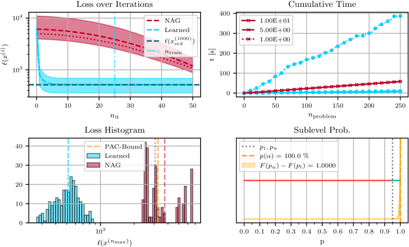
Results.
The upper left plot of Figure 6 shows that the learned algorithm outperforms HBF by orders of magnitude and, despite being trained for iterations, one can use it for at least 700 iterations in most cases (). However, the mean indicates that there are single instances for which instabilities occur, and, by comparing it to the median, one observes that the mean is far from being representative of the “typical” performance. Further, the algorithm performs well on very different orders of magnitude, ranging from to . The upper right plot confirms that also in terms of computation time the learned algorithm is way faster than heavy-ball, and the lower left plot shows that the predicted PAC-bound is quite tight. Lastly, the lower right plot shows that the algorithm will not converge in all of the cases, yet satisfies the specified constraints and .
6.2 Image Processing
We consider (gray-scale) image denoising/deblurring with a regularizer given as smooth approximation to the -norm of the image derivative, that is, problems of the form:
The matrix describes the “blurring” of the image, while and are the discrete image derivatives in h- and w-direction, respectively, which are used to penalize local changes in the image. We use images of height and width . Thus, the dimension of the optimization space is given by . Further, as parameters we use the observed image and the regularization parameter, that is, .
Construction of the Parameters.
Throughout, we use . For computational efficiency, the matrices are implemented through the convolution of the image with a corresponding kernel (with reflective boundary conditions). For , we use a standard -Gaussian kernel, while and are given through the kernels:
Additionally, after blurring an image with , we add centered Gaussian noise with standard deviation to each pixel, that is, with , , . The regularization parameters , , are given by sampling uniformly, that is, , where we use and .
Baseline.
Since the problem is smooth and convex, yet not strongly convex, the baseline algorithm is given by the accelerated gradient descent algorithm due to Nesterov (1983). Its update is given by first computing followed by setting . We use the optimal choices and . Here, the smoothness constant is given by the largest eigenvalue of , where is given by “stacking” and , that is, .
Algorithm.
The algorithmic update of is visualized in Figure 7 and consists of an update-block, which combines , and their “interaction” into the new update direction , and a block to compute a step-size from the norms of the gradient and momentum term. Note that we use -convolutions this time, that is, we incorporate the knowledge about an image-processing problem into the design of the optimization algorithm.
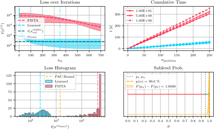
Results.
The results of this experiment are summarized in Figure 8. The upper left plot shows that the learned algorithm is much faster than NAG in terms of the loss over the iterations, reaching a loss close to the ground-truth after only 5 iterations. The upper right plot confirms this finding also in terms of computation time. Yet, one can observe a strong increase in computation time for the dotted line (loss per pixel of about ), indicating that the learned algorithm often is not able to reach this accuracy. In the lower left plot, one can observe that the predicted PAC-bound is not perfectly tight, yet provides the guarantee to outperform NAG. Finally, the lower right plot shows that the probabilistically constraint optimization/sampling procedure did work correctly, as the point estimate is equal to one, that is, the algorithm did reach the sublevel set in of the test cases.
6.3 Lasso-Problem
Here we consider the Lasso problem (Tibshirani, 1996), that is, a non-smooth problem of the form:
with . Thus, we are solving an overdetermined system of linear equations with an additional -regularization term, which promotes sparsity in the solution (see Hastie et al., 2009). Hence, the optimization variable is given by .
Construction of the Parameters.
The same matrix with dimensions and is used for all problem instances. Here, we sample each entry uniformly, that is, , , . Thus, the parameters are given by the right-hand side and the regularization parameter, that is, . For this, the regularization parameter is also sampled uniformly, that is, , , with and , while the right-hand side is sampled from a multivariate normal distribution, that is, , , where we first construct and by sampling each entry of and uniformly at random in .
Baseline.
We use the FISTA algorithm (Beck and Teboulle, 2009) as baseline, which performs an extrapolation step followed by a proximal gradient step, that is, abbreviating and , the update is given by first computing followed by setting . Here, the proximal mapping is defined as , and can be computed efficiently in closed-form yielding the so-called soft-thresholding operator:
We choose , where is the largest eigenvalue of , that is, the smoothness parameter of , while is set to with .
Algorithm.
The algorithmic update of the learned algorithm for this experiment is visualized in Figure 9 and consists of three blocks: First, an update-block, which combines the directions , , their interaction , and the direction (of the -norm) into an update direction . Second, a block to compute a step-size based on the norms of the gradient, subgradient and momentum term. And a final block, which is able to scale the single coordinates of a given point down, and, together with the proximal map, is used to promote sparsity in the solution. However, by appropriate scaling afterwards we ensure that the proximal map does not change the norm of the given point, to avoid that the network reduces the loss by just putting coordinates to zero.
Results.
The results of this experiment are summarized in Figure 10. The upper left plot shows that the learned algorithm outperforms FISTA by several orders of magnitude, achieving a loss that is slightly smaller than the one of after only 200 iterations, and one can observe that the learned algorithm can be used for more iterations than it was trained for. The upper right plot confirms that it is also way faster in terms of computation time. Yet, the increase in computation time for the dotted line indicates an increased difficulty to reach the level of accuracy, that is, might not reach arbitrary levels of accuracy. The lower left plot shows that the predicted PAC-bound is not perfectly tight here, yet guarantees that will outperform FISTA on average. And the lower right plot indicates that the probabilistically constrained optimization/sampling procedure did work as intended, since the algorithm did reach the sublevel set in all of the test cases.
6.4 Training Neural Networks
This experiment considers the problem of training a neural network on a regression problem, that is, is trained to predict the parameters of a neural network , which then is used to predict a function . Hence, the optimization variable is given by .
Construction of the Parameters.
We assume that the neural network should learn a function from noisy observations , that is with . For this, we construct polynomials , , of degree as follows: For every function , we sample points (here: ) uniformly in , that is, , , . Then, we sample the coefficients of uniformly in , that is, , , . Lastly, we get the values as:
For every function the neural network is trained on the data set with and . Hence, the data set will serve as the parameter of the loss function , such that the parameter space can be identified as the space of these data sets, that is, .
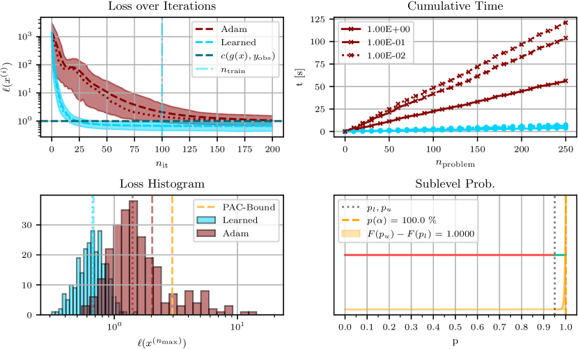
Loss Function.
Since the mean square error is the standard choice for training models on regression tasks, the loss is given by .
Architecture.
As model we use a fully-connected two layer neural network with ReLU-activation functions. To have more features in the input layer, the input is transformed into the vector . Hence, the parameters are given by the weights and biases of the two fully-connected layers. Therefore, the optimization space is of dimension .
Baseline.
As baseline we use Adam (Kingma and Ba, 2015) (as it is implemented in PyTorch), which is a widely used optimization algorithms for training neural networks. For tuning, we perform a grid search over 100 step-size parameters, such that its performance is best for the given iterations. Note that originally Adam was introduced for stochastic optimization, while we use it in the “full-batch setting” here, that is, without stochasticity.
Algorithm.
The algorithmic update in Figure 11 consists of two blocks: A weighting block, which computes four weights based on the norms , the losses , and the scalar product . Each of these gets multiplied with , or the “pre-conditioned” versions, which we compute by pointwise multiplication with the learned vectors and . Then, additionally to the and , these weighted directions get fed into an update-block, which computes the final update direction .
Results.
The upper left plot of Figure 12 shows that the learned algorithm clearly outperforms Adam, reaching the ground-truth loss after about 25 iterations, while Adam is not able to reach it within 200 iterations. Further, while the algorithm was trained for 100 iterations, it can be applied for more. The upper right plot confirms that also in terms of computation time is way faster in training the neural network than Adam, and, as the learned algorithm goes below the ground-truth loss at around 25 iterations, all three levels of accuracy are reached similarly fast. The lower left plot shows that the predicted PAC-bound is not perfectly tight, yet yields a reasonable bound on the average performance, and guarantees to perform at least as good as Adam (on average). The lower right plot indicates that the probabilistically constrained optimization/sampling procedure did work correctly, as the algorithm did reach the sublevel set in all test cases.
7 Discussion and Limitations
The motivation for this paper was to use more structure in a given problem than is analytically tractable. For this, we considered a distribution over parametric loss functions and formulated the (ultimate) goal in (1), that is, to find a solution to each realization from this distribution. Under reasonable assumptions, this problem is too general to be solved. This led to the formulation of the performance of an algorithm in terms of its risk. However, since this is intractable, we derived PAC-Bayesian generalization bounds relating the risk to the empirically observable performance on a data set. This resulted in the formulation of a training objective, which relies heavily on the existence of a prior distribution satisfying our assumptions and yielding a good performance. As such a distribution is typically not known, we derived a procedure to construct it. This involved several key choices, including the loss-function, specific randomization steps, and, especially, the probabilistic constraints. Finally, we validated the resulting learning procedure on four practically relevant problems and showed that it yields a superior performance. While these experimental results are promising, we nevertheless see four main limitations of our work. First, the only guarantee that is provided by the PAC-Bayesian bound is an upper bound on the function value after a specified number of iterations. In particular, it does not guarantee that the function values, the iterates, or the gradient norm actually do converge. Second, our learning procedure is not guaranteed to work and still involves many design choices. Third, one still has to find a good architecture for each given problem, which can be time-consuming. Fourth, the presented algorithmic procedure is quite elaborate, and its implementation is tedious. Additionally, the training procedure (offline) has a high computational cost, which, at least in part, however, is due to the nature of learning-to-optimize. All these are promising directions of research that we leave to a future work.
Acknowledgments and Disclosure of Funding
M. Sucker and P. Ochs acknowledge funding by the German Research Foundation under Germany’s Excellence Strategy – EXC number 2064/1 – 390727645. Furthermore, J. Fadili and P. Ochs are supported by the ANR-DFG joint project TRINOM-DS under the numbers ANR-20-CE92-0037-01 and OC150/5-1.
Appendix A Supplementary Definitions
Definition A.1 (Probability Kernel)
Let , be measurable spaces. A function is called a kernel from to , written as , if for every set , the map is measurable, and for every point , the map is a measure. Furthermore, is called a probability kernel from to , if for every .
Definition A.2 (Polish space)
A topological space is said to be Polish if it is separable and admits a complete metrization.
Remark A.3
Examples of Polish spaces are countable discrete spaces, with the standard topology, separable Banach spaces with the norm toplogy, or countable products of Polish spaces.
Definition A.4 (Exponential Family)
Let be a non-empty index set. A family of probability measures on a measurable space is called an exponential family (in and ), if there is a dominating probability measure , that is, , functions , , and measurable functions , , such that for every we have , that is, , .
Definition A.5 (Support of a Measure)
Let be a topological space, and let be a measure on . The support of is defined as:
Remark A.6
The support of a measure is closed, that is, Borel measurable, and satisfies .
Appendix B Supplementary Lemmas
Lemma B.1
Under Assumption 2.12, is a data-dependent distribution for every .
Proof
Denote the density of w.r.t. by . The map is measurable, as is measurable w.r.t. the product--algebra and is a finite measure (Kallenberg, 2021, Lemma 1.28, p.25). Hence, is measurable w.r.t. , since . Thus, it holds that is a kernel from from to (Kallenberg, 2021, Lem. 3.2, p.56). Finally, is actually a probability kernel, since is the corresponding normalization constant.
Since the loss-function is neither assumed to be bounded nor to satisfy any self-bounding or bounded-difference property, the following result is needed. It states that non-negative random variables with finite second moment satisfy a one-sided sub-Gaussian inequality. It can be found as Exercise 2.9 on page 47 in Boucheron et al. (2013).
Lemma B.2
Let be a non-negative random variable with finite second moment. Then, for every it holds .
Lemma B.3
The sublevel set is measurable.
Proof
As is assumed to be measurable, it suffices to show that the specific composition of and is measurable, that is, is measurable w.r.t. and . Since is measurable, there exists a sequence of simple333A function is called simple, if it is of the form with disjoint sets . functions with . Thus, since limits of measurable functions are measurable, it suffices to consider the case of a simple function . Then, however, since addition and multiplication are measurable, it suffices to consider characteristic functions of the form for a measurable set . Since the product--algebra is generated by cylinder sets of the form with , , it actually suffices to consider the case , that is, . The second term is obviously measurable, and the first term is measurable as a (standard) composition of two measurable functions. Therefore, the conclusion follows.
Appendix C Proof of Lemma 3.1
Proof Take any and . First, let be arbitrary. By the Radon-Nikodym theorem, there exists a measurable function , s.t. . Since the convention applies throughout measure theory, one has:
Hence, w.l.o.g. we can assume that -a.s. Then, by Jensen’s inequality, one gets:
Hence, we have for any probability measure . Now consider the member of the exponential family:
Rearranging yields .
Appendix D Proof of Lemma 3.2
Proof W.l.o.g. assume that and choose , . Then, for every , it holds that:
Thus, in total one gets for :
Taking gives .
Appendix E Proof of Corollary 3.5
Proof The two forumlas are simply rewritings of each other: By assumption, bilinearity and definition of the euclidean scalar product, and linearity of the integral, the term can be split up as:
Simply rearranging the terms then yields the result, as .
References
- Alquier (2008) Pierre Alquier. PAC-Bayesian bounds for randomized empirical risk minimizers. Mathematical Methods of Statistics, 17(4):279–304, 2008.
- Alquier (2021) Pierre Alquier. User-friendly introduction to PAC-Bayes bounds. arXiv preprint arXiv:2110.11216, 2021.
- Alquier and Guedj (2018) Pierre Alquier and Benjamin Guedj. Simpler PAC-Bayesian bounds for hostile data. Machine Learning, 107(5):887–902, 2018.
- Alquier et al. (2016) Pierre Alquier, James Ridgway, and Nicolas Chopin. On the properties of variational approximations of Gibbs posteriors. Journal of Machine Learning Research, 17(1):8374–8414, 2016.
- Amit et al. (2022) Ron Amit, Baruch Epstein, Shay Moran, and Ron Meir. Integral probability metrics PAC-Bayes bounds. Advances in Neural Information Processing Systems, 35:3123–3136, 2022.
- Andrychowicz et al. (2016) Marcin Andrychowicz, Misha Denil, Sergio Gomez, Matthew W Hoffman, David Pfau, Tom Schaul, Brendan Shillingford, and Nando De Freitas. Learning to learn by gradient descent by gradient descent. Advances in neural information processing systems, 29, 2016.
- Bardenet et al. (2014) Rémi Bardenet, Arnaud Doucet, and Chris Holmes. Towards scaling up markov chain monte carlo: an adaptive subsampling approach. In International conference on machine learning, pages 405–413. PMLR, 2014.
- Bardenet et al. (2017) Rémi Bardenet, Arnaud Doucet, and Chris Holmes. On Markov chain Monte Carlo methods for tall data. Journal of Machine Learning Research, 18(47), 2017.
- Barndorff–Nielsen (2014) Ole Barndorff–Nielsen. Information and exponential families: in statistical theory. John Wiley & Sons, 2014.
- Beck and Teboulle (2009) Amir Beck and Marc Teboulle. A fast iterative shrinkage-thresholding algorithm for linear inverse problems. SIAM journal on imaging sciences, 2(1):183–202, 2009.
- Bégin et al. (2016) Luc Bégin, Pascal Germain, François Laviolette, and Jean-Francis Roy. PAC-Bayesian bounds based on the Rényi divergence. In Artificial Intelligence and Statistics, pages 435–444. PMLR, 2016.
- Berger (1985) James O. Berger. Statistical decision theory and Bayesian analysis. Springer-Verlag, 1985.
- Bianchi et al. (2022) Pascal Bianchi, Walid Hachem, and Sholom Schechtman. Convergence of constant step stochastic gradient descent for non-smooth non-convex functions. Set-Valued and Variational Analysis, pages 1–31, 2022.
- Bolte and Pauwels (2021) Jérôme Bolte and Edouard Pauwels. Conservative set valued fields, automatic differentiation, stochastic gradient methods and deep learning. Mathematical Programming, 188(1):19–51, 2021.
- Bottou et al. (2018) Leon Bottou, Frank E Curtis, and Jorge Nocedal. Optimization methods for large-scale machine learning. Siam Review, 60(2):223–311, 2018.
- Boucheron et al. (2013) Stephane Boucheron, Gabor Lugosi, and Pascal Massart. Concentration inequalities: A nonasymptotic theory of independence. Oxford university press, 2013.
- Bousquet and Elisseeff (2000) Olivier Bousquet and André Elisseeff. Algorithmic stability and generalization performance. Advances in Neural Information Processing Systems, 13, 2000.
- Bousquet and Elisseeff (2002) Olivier Bousquet and André Elisseeff. Stability and generalization. Journal of Machine Learning Research, 2:499–526, 2002.
- Buzzard et al. (2018) Gregery T Buzzard, Stanley H Chan, Suhas Sreehari, and Charles A Bouman. Plug-and-play unplugged: Optimization-free reconstruction using consensus equilibrium. SIAM Journal on Imaging Sciences, 11(3):2001–2020, 2018.
- Catoni (2004) Olivier Catoni. Statistical learning theory and stochastic optimization: Ecole d’Eté de Probabilités de Saint-Flour, XXXI-2001, volume 1851. Springer Science & Business Media, 2004.
- Catoni (2007) Olivier Catoni. PAC-Bayesian supervised classification: The thermodynamics of statistical learning. Lecture Notes-Monograph Series, 56:i–163, 2007.
- Chan et al. (2016) Stanley H Chan, Xiran Wang, and Omar A Elgendy. Plug-and-play ADMM for image restoration: Fixed-point convergence and applications. IEEE Transactions on Computational Imaging, 3(1):84–98, 2016.
- Chen et al. (2020a) Tianlong Chen, Weiyi Zhang, Zhou Jingyang, Shiyu Chang, Sijia Liu, Lisa Amini, and Zhangyang Wang. Training stronger baselines for learning to optimize. Advances in Neural Information Processing Systems, 33:7332–7343, 2020a.
- Chen et al. (2021) Tianlong Chen, Xiaohan Chen, Wuyang Chen, Howard Heaton, Jialin Liu, Zhangyang Wang, and Wotao Yin. Learning to optimize: A primer and a benchmark. arXiv preprint arXiv:2103.12828, 2021.
- Chen et al. (2018) Xiaohan Chen, Jialin Liu, Zhangyang Wang, and Wotao Yin. Theoretical linear convergence of unfolded ISTA and its practical weights and thresholds. Advances in Neural Information Processing Systems, 31, 2018.
- Chen et al. (2020b) Xinshi Chen, Yufei Zhang, Christoph Reisinger, and Le Song. Understanding deep architecture with reasoning layer. Advances in Neural Information Processing Systems, 33:1240–1252, 2020b.
- Chen et al. (2017) Yutian Chen, Matthew W Hoffman, Sergio Gómez Colmenarejo, Misha Denil, Timothy P Lillicrap, Matt Botvinick, and Nando Freitas. Learning to learn without gradient descent by gradient descent. In International Conference on Machine Learning, pages 748–756. PMLR, 2017.
- Cohen et al. (2021) Regev Cohen, Michael Elad, and Peyman Milanfar. Regularization by denoising via fixed-point projection. SIAM Journal on Imaging Sciences, 14(3):1374–1406, 2021.
- Davis and Drusvyatskiy (2019) Damek Davis and Dmitriy Drusvyatskiy. Stochastic model-based minimization of weakly convex functions. SIAM Journal on Optimization, 29(1):207–239, 2019.
- Davis and Drusvyatskiy (2022) Damek Davis and Dmitriy Drusvyatskiy. Graphical convergence of subgradients in nonconvex optimization and learning. Mathematics of Operations Research, 47(1):209–231, 2022.
- Défossez et al. (2022) Alexandre Défossez, Leon Bottou, Francis Bach, and Nicolas Usunier. A simple convergence proof of adam and adagrad. Transactions on Machine Learning Research, 2022. ISSN 2835-8856.
- Donsker and Varadhan (1975) Monroe D Donsker and SR Srinivasa Varadhan. Asymptotic evaluation of certain Markov process expectations for large time, i. Communications on Pure and Applied Mathematics, 28(1):1–47, 1975.
- Dziugaite and Roy (2017) Gintare Karolina Dziugaite and Daniel M. Roy. Computing nonvacuous generalization bounds for deep (stochastic) neural networks with many more parameters than training data. In Proceedings of the Thirty-Third Conference on Uncertainty in Artificial Intelligence, UAI 2017, Sydney, Australia, August 11-15, 2017. AUAI Press, 2017.
- Dziugaite and Roy (2018) Gintare Karolina Dziugaite and Daniel M Roy. Data-dependent PAC-Bayes priors via differential privacy. Advances in neural information processing systems, 31, 2018.
- Dziugaite et al. (2021) Gintare Karolina Dziugaite, Kyle Hsu, Waseem Gharbieh, Gabriel Arpino, and Daniel Roy. On the role of data in PAC-Bayes bounds. In International Conference on Artificial Intelligence and Statistics, pages 604–612. PMLR, 2021.
- Efron (1975) Bradley Efron. Defining the curvature of a statistical problem (with applications to second order efficiency). The Annals of Statistics, pages 1189–1242, 1975.
- Germain et al. (2009) Pascal Germain, Alexandre Lacasse, François Laviolette, and Mario Marchand. PAC-Bayesian learning of linear classifiers. In Proceedings of the 26th Annual International Conference on Machine Learning, pages 353–360, 2009.
- Gregor and LeCun (2010) Karol Gregor and Yann LeCun. Learning fast approximations of sparse coding. In Proceedings of the 27th international conference on international conference on machine learning, pages 399–406, 2010.
- Guedj (2019) Benjamin Guedj. A primer on PAC-Bayesian learning. In Proceedings of the second congress of the French Mathematical Society, volume 33, 2019.
- Haddouche and Guedj (2023) Maxime Haddouche and Benjamin Guedj. Wasserstein PAC-Bayes learning: Exploiting optimisation guarantees to explain generalisation, 2023.
- Hastie et al. (2009) Trevor Hastie, Robert Tibshirani, and Jerome Friedman. The elements of statistical learning: data mining, inference and prediction. Springer, 2 edition, 2009.
- He et al. (2021) Xin He, Kaiyong Zhao, and Xiaowen Chu. Automl: A survey of the state-of-the-art. Knowledge-Based Systems, 212:106622, 2021.
- Honorio and Jaakkola (2014) Jean Honorio and Tommi Jaakkola. Tight bounds for the expected risk of linear classifiers and PAC-Bayes finite-sample guarantees. In Artificial Intelligence and Statistics, pages 384–392. PMLR, 2014.
- Hospedales et al. (2021) Timothy Hospedales, Antreas Antoniou, Paul Micaelli, and Amos Storkey. Meta-learning in neural networks: A survey. IEEE transactions on pattern analysis and machine intelligence, 44(9):5149–5169, 2021.
- Hutter et al. (2019) Frank Hutter, Lars Kotthoff, and Joaquin Vanschoren. Automated machine learning: methods, systems, challenges. Springer Nature, 2019.
- Kallenberg (2021) O. Kallenberg. Foundations of Modern Probability. Probability theory and stochastic modelling. Springer, 2021. ISBN 9783030618728.
- Kavis et al. (2022) Ali Kavis, Kfir Yehuda Levy, and Volkan Cevher. High probability bounds for a class of nonconvex algorithms with adagrad stepsize. In International Conference on Learning Representations, 2022. URL https://openreview.net/forum?id=dSw0QtRMJkO.
- Kingma and Ba (2015) Diederik P. Kingma and Jimmy Ba. Adam: A method for stochastic optimization. In 3rd International Conference on Learning Representations, ICLR 2015, 2015.
- Klenke (2013) Achim Klenke. Wahrscheinlichkeitstheorie. Springer Spektrum, 2013.
- Kobler et al. (2020) Erich Kobler, Alexander Effland, Karl Kunisch, and Thomas Pock. Total deep variation: A stable regularizer for inverse problems. arXiv preprint arXiv:2006.08789, 2020.
- Korattikara et al. (2014) Anoop Korattikara, Yutian Chen, and Max Welling. Austerity in MCMC land: Cutting the Metropolis-Hastings budget. In International conference on machine learning, pages 181–189. PMLR, 2014.
- Langford and Caruana (2001) John Langford and Rich Caruana. (Not) bounding the true error. In T. Dietterich, S. Becker, and Z. Ghahramani, editors, Advances in Neural Information Processing Systems, volume 14. MIT Press, 2001.
- Langford and Shawe-Taylor (2002) John Langford and John Shawe-Taylor. PAC-Bayes and margins. Advances in neural information processing systems, 15, 2002.
- Lever et al. (2013) Guy Lever, François Laviolette, and John Shawe-Taylor. Tighter PAC-Bayes bounds through distribution-dependent priors. Theoretical Computer Science, 473:4–28, 2013.
- London (2017) Ben London. A PAC-Bayesian analysis of randomized learning with application to stochastic gradient descent. Advances in Neural Information Processing Systems, 30, 2017.
- Lv et al. (2017) Kaifeng Lv, Shunhua Jiang, and Jian Li. Learning gradient descent: Better generalization and longer horizons. In International Conference on Machine Learning, pages 2247–2255. PMLR, 2017.
- Maclaurin and Adams (2014) Dougal Maclaurin and Ryan P Adams. Firefly Monte Carlo: Exact MCMC with subsets of data. In 30th Conference on Uncertainty in Artificial Intelligence, UAI 2014, pages 543–552. AUAI Press, 2014.
- McAllester (2003a) David McAllester. Simplified PAC-Bayesian margin bounds. In Learning theory and Kernel machines, pages 203–215. Springer, 2003a.
- McAllester (2003b) David McAllester. PAC-Bayesian stochastic model selection. Machine Learning, 51(1):5–21, 2003b.
- Metz et al. (2019) Luke Metz, Niru Maheswaranathan, Jeremy Nixon, Daniel Freeman, and Jascha Sohl-Dickstein. Understanding and correcting pathologies in the training of learned optimizers. In Proceedings of the 36th International Conference on Machine Learning, volume 97 of Proceedings of Machine Learning Research, pages 4556–4565. PMLR, 2019.
- Moeller et al. (2019) Michael Moeller, Thomas Mollenhoff, and Daniel Cremers. Controlling neural networks via energy dissipation. In Proceedings of the IEEE/CVF International Conference on Computer Vision, pages 3256–3265, 2019.
- Nesterov (1983) Yurii Nesterov. A method for solving the convex programming problem with convergence rate . Proceedings of the USSR Academy of Sciences, 269:543–547, 1983.
- Nesterov (2018) Yurii Nesterov. Lectures on convex optimization, volume 137. Springer, 2018.
- Ohnishi and Honorio (2021) Yuki Ohnishi and Jean Honorio. Novel change of measure inequalities with applications to PAC-Bayesian bounds and Monte Carlo estimation. In International Conference on Artificial Intelligence and Statistics, pages 1711–1719. PMLR, 2021.
- Parrado-Hernández et al. (2012) Emilio Parrado-Hernández, Amiran Ambroladze, John Shawe-Taylor, and Shiliang Sun. PAC-Bayes bounds with data dependent priors. Journal of Machine Learning Research, 13(1):3507–3531, 2012.
- Paszke et al. (2019) Adam Paszke, Sam Gross, Francisco Massa, Adam Lerer, James Bradbury, Gregory Chanan, Trevor Killeen, Zeming Lin, Natalia Gimelshein, Luca Antiga, Alban Desmaison, Andreas Kopf, Edward Yang, Zachary DeVito, Martin Raison, Alykhan Tejani, Sasank Chilamkurthy, Benoit Steiner, Lu Fang, Junjie Bai, and Soumith Chintala. Pytorch: An imperative style, high-performance deep learning library. In Advances in Neural Information Processing Systems, volume 32. Curran Associates, Inc., 2019.
- Pérez-Ortiz et al. (2021) María Pérez-Ortiz, Omar Rivasplata, John Shawe-Taylor, and Csaba Szepesvári. Tighter risk certificates for neural networks. Journal of Machine Learning Research, 22(227):1–40, 2021.
- Polyak (1964) Boris T Polyak. Some methods of speeding up the convergence of iteration methods. USSR Computational Mathematics and Mathematical Physics, 4(5):1–17, 1964.
- Quiroz et al. (2018) Matias Quiroz, Robert Kohn, Mattias Villani, and Minh-Ngoc Tran. Speeding up MCMC by efficient data subsampling. Journal of the American Statistical Association, 2018.
- Rivasplata et al. (2020) Omar Rivasplata, Ilja Kuzborskij, Csaba Szepesvári, and John Shawe-Taylor. PAC-Bayes analysis beyond the usual bounds. Advances in Neural Information Processing Systems, 33:16833–16845, 2020.
- Robert and Casella (2004) C.P. Robert and G. Casella. Monte Carlo statistical methods. Springer New York, 2004.
- Ryu et al. (2019) Ernest Ryu, Jialin Liu, Sicheng Wang, Xiaohan Chen, Zhangyang Wang, and Wotao Yin. Plug-and-play methods provably converge with properly trained denoisers. In International Conference on Machine Learning, pages 5546–5557. PMLR, 2019.
- Seeger (2002) Matthias Seeger. PAC-Bayesian generalisation error bounds for Gaussian process classification. Journal of Machine Learning Research, 3:233–269, 2002.
- Shalev-Shwartz et al. (2009) Shai Shalev-Shwartz, Ohad Shamir, Nathan Srebro, and Karthik Sridharan. Stochastic convex optimization. In COLT, volume 2, page 5, 2009.
- Shalev-Shwartz et al. (2010) Shai Shalev-Shwartz, Ohad Shamir, Nathan Srebro, and Karthik Sridharan. Learnability, stability and uniform convergence. Journal of Machine Learning Research, 11:2635–2670, 2010.
- Sreehari et al. (2016) Suhas Sreehari, S Venkat Venkatakrishnan, Brendt Wohlberg, Gregery T Buzzard, Lawrence F Drummy, Jeffrey P Simmons, and Charles A Bouman. Plug-and-play priors for bright field electron tomography and sparse interpolation. IEEE Transactions on Computational Imaging, 2(4):408–423, 2016.
- Sucker and Ochs (2023) Michael Sucker and Peter Ochs. PAC-Bayesian learning of optimization algorithms. In International Conference on Artificial Intelligence and Statistics, pages 8145–8164. PMLR, 2023.
- Sun et al. (2019) Yu Sun, Brendt Wohlberg, and Ulugbek S Kamilov. An online plug-and-play algorithm for regularized image reconstruction. IEEE Transactions on Computational Imaging, 5(3):395–408, 2019.
- Teodoro et al. (2017) Afonso M Teodoro, José M Bioucas-Dias, and Mário AT Figueiredo. Scene-adapted plug-and-play algorithm with convergence guarantees. In 2017 IEEE 27th International Workshop on Machine Learning for Signal Processing (MLSP), pages 1–6. IEEE, 2017.
- Terris et al. (2021) Matthieu Terris, Audrey Repetti, Jean-Christophe Pesquet, and Yves Wiaux. Enhanced convergent PNP algorithms for image restoration. In 2021 IEEE International Conference on Image Processing (ICIP), pages 1684–1688. IEEE, 2021.
- Thiemann et al. (2017) Niklas Thiemann, Christian Igel, Olivier Wintenberger, and Yevgeny Seldin. A strongly quasiconvex PAC-Bayesian bound. In International Conference on Algorithmic Learning Theory, pages 466–492. PMLR, 2017.
- Tibshirani (1996) Robert Tibshirani. Regression shrinkage and selection via the LASSO. Journal of the Royal Statistical Society Series B: Statistical Methodology, 58(1):267–288, 1996.
- Tirer and Giryes (2018) Tom Tirer and Raja Giryes. Image restoration by iterative denoising and backward projections. IEEE Transactions on Image Processing, 28(3):1220–1234, 2018.
- Vilalta and Drissi (2002) Ricardo Vilalta and Youssef Drissi. A perspective view and survey of meta-learning. Artificial intelligence review, 18:77–95, 2002.
- Villani et al. (2009) Cédric Villani et al. Optimal transport: old and new, volume 338. Springer, 2009.
- Welling and Teh (2011) Max Welling and Yee W Teh. Bayesian learning via stochastic gradient Langevin dynamics. In Proceedings of the 28th international conference on machine learning (ICML), pages 681–688, 2011.
- Wichrowska et al. (2017) Olga Wichrowska, Niru Maheswaranathan, Matthew W Hoffman, Sergio Gomez Colmenarejo, Misha Denil, Nando Freitas, and Jascha Sohl-Dickstein. Learned optimizers that scale and generalize. In International conference on machine learning, pages 3751–3760. PMLR, 2017.
- Witting (2013) Hermann Witting. Mathematische Statistik I: Parametrische Verfahren bei festem Stichprobenumfang. Springer-Verlag, 2013.
- Xin et al. (2016) Bo Xin, Yizhou Wang, Wen Gao, David Wipf, and Baoyuan Wang. Maximal sparsity with deep networks? Advances in Neural Information Processing Systems, 29, 2016.
- Yao et al. (2018) Quanming Yao, Mengshuo Wang, Yuqiang Chen, Wenyuan Dai, Yu-Feng Li, Wei-Wei Tu, Qiang Yang, and Yang Yu. Taking human out of learning applications: A survey on automated machine learning. arXiv preprint arXiv:1810.13306, 2018.