MMSE Channel Estimation in Large-Scale MIMO: Improved Robustness with Reduced Complexity

Abstract

Large-scale MIMO systems with a massive number $N$ of individually controlled antennas pose significant challenges for minimum mean square error (MMSE) channel estimation, based on uplink pilots. The major ones arise from the computational complexity, which scales with $N^{3}$, and from the need for accurate knowledge of the channel statistics. This paper aims to address both challenges by introducing reduced-complexity channel estimation methods that achieve the performance of MMSE in terms of estimation accuracy and uplink spectral efficiency while demonstrating improved robustness in practical scenarios where channel statistics must be estimated. This is achieved by exploiting the inherent structure of the spatial correlation matrix induced by the array geometry. Specifically, we use a Kronecker decomposition for uniform planar arrays and a well-suited circulant approximation for uniform linear arrays. By doing so, a significantly lower computational complexity is achieved, scaling as $N\sqrt{N}$ and $N\log N$ for squared planar arrays and linear arrays, respectively.

Sect. I Introduction and motivation

Communications theorists are always looking for new technologies to improve the speed and reliability of wireless communications. Among these technologies, the multiple antenna technology has made significant advances, with the latest implementation being massive multiple-input multiple-output (MIMO) [2], introduced with the advent of 5G [3]. Researchers are now exploring improved deployment methods for massive MIMO, incorporating more antennas and optimized signal processing algorithms to take advantage of its potential benefits. This evolution of massive MIMO has been referred to as massive MIMO 2.0 [4], leading to the exploration of MIMO systems with extremely larger antenna arrays. This is referred to as X-MIMO in industry terminology. Various terms, such as extremely large aperture arrays [3], extremely large-scale MIMO (XL-MIMO) [5], and ultra-massive MIMO (UM-MIMO) [6], have also been suggested in academic literature. In this paper, we simply use the large-scale MIMO terminology.

Accurate channel state information (CSI) is crucial for the efficient use of large-scale MIMO, enabling precise transmission beamforming in downlink (DL) and coherent signal combining in uplink (UL). The basic way to acquire CSI in time-division duplexing systems is to transmit a predefined pilot sequence and estimate the channel coefficients at the base station (BS). However, performing MMSE channel estimation in a large-scale MIMO system with a massive number $N$ of antennas (e.g., in the order of thousands) poses critical challenges in the implementation of the MMSE estimator (whose computational complexity may scale as $N^{3}$ due to matrix inversion, e.g., [7, 8]) and in the acquisition of the channel statistics, i.e., the spatial correlation matrices. In practical communication scenarios, the latter are not known a priori and must be estimated based on observed channel measurements [2]. This is crucial for designing robust and efficient large-scale MIMO systems [4]. An alternative is to use the least-squares (LS) estimator [9], which requires neither matrix inversion nor statistical information. However, its performance is significantly inferior to MMSE, e.g., [2]. The objective of this paper is to tackle this challenge by developing channel estimation schemes that achieve accuracy levels comparable to the MMSE estimator, while also offering reduced complexity and enhanced robustness to the imperfect knowledge of channel statistics.

I-A Related work

A variety of schemes exists in the literature to achieve the same performance of MMSE while handling complexity that scales with the number of antennas. These include for example methods based on exhaustive search [10], hierarchical search [11, 12, 13], and compressed sensing (CS) [14, 15, 16]. The exhaustive method in [10] exploits a sequence of training symbols, whose overhead becomes prohibitively as the number $N$ of antennas increases. To overcome this issue, a hierarchical search based on a predefined codebook is proposed in [11, 12, 13]. However, while significantly reducing the complexity, the limited codebook size severely affects the estimation accuracy. Alternative methods to reduce the pilot overhead take advantage of CS techniques, which exploit the fact that the propagation channels of most practical communication scenarios can be sparsely represented in the angular domain. A parametric approach is used in [16] for line-of-sight (LoS) communications. A different approach is pursued in [17], which exploits the high rank deficiency observed in the spatial correlation matrices caused by the large-scale MIMO geometry [18], to derive a subspace-based channel estimation approach. The complexity saving is due to a compact eigenvalue decomposition, which lets the proposed reduced-subspace (RS-LS) estimator attain the MMSE performance when the pilot signal-to-noise ratio (SNR) becomes significantly large. However, this might not hold true, especially for practical transmitter-receiver distances.

The vast majority of the aforementioned literature assumes that the channel statistics are perfectly known. However, this assumption is questionable because the matrix dimensions grow with $N$ and the statistics change over time (e.g., due to mobility). Practical covariance estimates are imperfect because the number of observations may be comparable to $N$. One promising approach to estimating a large-dimensional covariance matrix with a small number of observations is to regularize the sample covariance matrix [19, 2]. This makes it scenario-dependent.

I-B Main contributions

This paper focuses on the development of channel estimation schemes that, compared to the optimal MMSE estimator, offer both lower computational complexity and improved robustness in the presence of imperfect knowledge of channel statistics. This is accomplished by exploiting the inherent structure of the spatial correlation matrix shaped by the array geometry, which is known in a given deployment scenario. For a uniform planar array (UPA), we use the Kronecker product decomposition [20, 21] to effectively separate the horizontal and vertical components within the array. For a uniform linear array (ULA), we use an appropriate circulant approximation [22, 23, 24], which allows the application of the discrete Fourier transform (DFT). Numerical results are used to evalute the effectiveness of the proposed methods in terms of normalized mean square estimation error (NMSE) and spectral efficiency (SE) in the uplink with different combining schemes. The results show that the proposed schemes achieve performance levels comparable to those with the MMSE estimator, while significantly reducing computational complexity. Specifically, the overall computational load, including the estimation of the spatial correlation matrices, scales as $N\sqrt{N}$ and $N\log N$ for squared planar arrays and linear arrays, respectively. Moreover, the schemes exhibit improved robustness in scenarios with imperfect knowledge of channel statistics, making them more suitable for dynamic environments. Remarkably, this is achieved without any regularization factor, making the schemes applicable without the need for fine-tuning according to the specific scenarios.

I-C Paper outline and notation

The remainder of the paper is structured as follows. Sect. II presents the system and channel models, whereas Sect. III revises the channel estimation problem in the presence of perfect knowledge of the channel statistics. Sects. IV and V derive low-complexity schemes for UPA and ULA scenarios, respectively. Sect. VI addresses the problem of estimating the channel statistics. Sects. VII and VIII investigate the complexity and the performance of the proposed schemes in terms of achievable SE in the uplink. Sect. IX concludes the paper.

Matrices and vectors are denoted by boldface uppercase and lowercase letters, respectively. The notation $\boldsymbol{\mathbf{A}}_{i,k}$ is used to indicate the $(i,k)$th entry of the enclosed matrix $\boldsymbol{\mathbf{A}}$, and $\boldsymbol{\mathbf{A}}=\mathrm{diag}\left({a(n);n=1,\dots,N}\right)$ denotes an $N\times N$ diagonal matrix with entries along its main diagonal. $\|\boldsymbol{\mathbf{x}}\|$ denotes the Euclidean norm of vector $\boldsymbol{\mathbf{x}}$, $\|\boldsymbol{\mathbf{A}}\|$ denotes the induced norm of matrix $\boldsymbol{\mathbf{A}}$, and $\|\boldsymbol{\mathbf{A}}\|_{\mathsf{F}}$ denotes the Frobenius norm of matrix $\boldsymbol{\mathbf{A}}$. Trace and rank of a matrix $\boldsymbol{\mathbf{A}}$ are denoted by $\mathrm{tr}\left({\boldsymbol{\mathbf{A}}}\right)$ and $\mathrm{rank}\left({\boldsymbol{\mathbf{A}}}\right)$, respectively, whereas $\boldsymbol{\mathbf{A}}^{\mathsf{T}}$ and $\boldsymbol{\mathbf{A}}^{\mathsf{H}}$ are the transpose and the conjugate transpose of $\boldsymbol{\mathbf{A}}$, respectively, with $\mathsf{j}$ denoting the imaginary unit. The $N\times N$ identity matrix and the all-zero vector with $N$ elements are denoted by $\boldsymbol{\mathbf{I}}_{N}$ and $\boldsymbol{\mathbf{0}}_{N}$, respectively. We use $\delta(\cdot)$ to denote the Dirac delta function, $\mathrm{mod}\left({\cdot,\cdot}\right)$ to denote the modulus operation, and $\lfloor\cdot\rfloor$ to truncate the argument, and $\otimes$ to indicate the Kronecker product.

I-D Reproducible research

The MatLab code used to obtain the simulation results will be made available upon completion of the review process.

Sect. II System and channel model

We consider a large-scale MIMO system with $K$ active user equipments. The BS is equipped with a UPA located in the $yz$ plane, and consisting of $N$ antennas, arranged into $N_{\mathsf{V}}$ rows, each hosting $N_{\mathsf{H}}$ radiating elements: $N=N_{\mathsf{H}}N_{\mathsf{V}}$. As illustrated in Figure 1, the inter-element spacing across horizontal and vertical directions is $\Delta_{\mathsf{H}}$ and $\Delta_{\mathsf{V}}$, respectively [25, Figure 1]. The location of the $n$th antenna, with $1\leq n\leq N$, with respect to the origin is $\boldsymbol{\mathbf{u}}_{n}=[0,i(n)\Delta_{\mathsf{H}},j(n)\Delta_{\mathsf{V}}]^{\mathsf{T}}$, where $i(n)=\mathrm{mod}\left({n-1,N_{\mathsf{H}}}\right)$ and $j(n)=\left\lfloor\left(n-1\right)/N_{\mathsf{H}}\right\rfloor$ are the horizontal and vertical indices of element $n$.

We call $\boldsymbol{\mathbf{h}}_{k}\in\mathbb{C}^{N}$ the channel vector between the single-antenna UE $k$ and the BS, and model it as [26]

$$\boldsymbol{\mathbf{h}}_{k}=\iint_{-\pi/2}^{\pi/2}g_{k}(\varphi,\theta)\boldsymbol{\mathbf{a}}(\varphi,\theta)d\varphi d\theta$$ (1)

where $\boldsymbol{\mathbf{a}}(\varphi,\theta)$ is the array response vector [2, Sect. 7.3]

$$\boldsymbol{\mathbf{a}}(\varphi,\theta)=\left[e^{\mathsf{j}\boldsymbol{\mathbf{k}}(\varphi,\theta)^{\mathsf{T}}\boldsymbol{\mathbf{u}}_{1}},\dots,e^{\mathsf{j}\boldsymbol{\mathbf{k}}(\varphi,\theta)^{\mathsf{T}}\boldsymbol{\mathbf{u}}_{N}}\right]^{\mathsf{T}}$$ (2)

of the UPA from azimuth angle $\varphi$ and elevation angle $\theta$, where $\boldsymbol{\mathbf{k}}(\varphi,\theta)=\frac{2\pi}{\lambda}\left[\cos(\theta)\cos(\varphi),\,\cos(\theta)\sin(\varphi),\,\sin(\theta)\right]^{\mathsf{T}}$ is the wave vector at wavelength $\lambda$. Also, $g_{k}(\varphi,\theta)$ is the angular spreading function.

\begin{overpic}[width=390.25534pt]{figures_final/fig01} \put(6.0,4.0){\footnotesize{$x$}} \put(92.0,24.0){\footnotesize{$y$}} \put(23.0,76.0){\footnotesize{$z$}} \put(43.0,73.0){\small{$N_{\mathsf{H}}$ columns}} \put(72.0,16.0){\footnotesize{$\Delta_{\mathsf{H}}$}} \put(13.0,39.0){\rotatebox{90.0}{\small{$N_{\mathsf{V}}$ rows}}} \put(91.0,55.0){\rotatebox{90.0}{\footnotesize{$\Delta_{\mathsf{V}}$}}} \put(62.0,12.0){\small{\acs{UE}}} \put(29.0,10.0){\footnotesize{$\varphi$}} \put(47.5,15.0){\footnotesize{$\theta$}} \put(2.0,13.0){\footnotesize{$\boldsymbol{\mathbf{u}}_{1}$}} \put(88.0,71.0){\footnotesize{$\boldsymbol{\mathbf{u}}_{N}$}} \end{overpic}

Figure 1: Diagram of the UPA located in the $yz$-plane, with a planar wave impinging with elevation $\theta$ and azimuth $\varphi$.

We consider the conventional block-fading model, where the channel $\boldsymbol{\mathbf{h}}_{k}$ is constant within one time-frequency block and takes independent realizations across blocks from a stationary stochastic distribution. In accordance with [26], we model $g_{k}(\varphi,\theta)$ as a spatially uncorrelated circularly symmetric Gaussian stochastic process with cross-correlation

$$\mathbb{E}\left\{{g_{k}(\varphi,\theta)g_{k}^{*}(\varphi^{\prime},\theta^{\prime})}\right\}=\beta_{k}f_{k}(\varphi,\theta)\delta(\varphi-\varphi^{\prime})\delta(\theta-\theta^{\prime})$$ (3)

where $\beta_{k}$ is the average channel gain and $f_{k}(\varphi,\theta)$ is the normalized spatial scattering function [26] such that $\iint f_{k}(\varphi,\theta)d\theta d\varphi=1$. By using (2), the elements of $\boldsymbol{\mathbf{R}}_{k}=\mathbb{E}\{\boldsymbol{\mathbf{h}}_{k}\boldsymbol{\mathbf{h}}_{k}^{\mathsf{H}}\}$ are computed as [2, Sect. 7.3.2]

$$[\boldsymbol{\mathbf{R}}_{k}]_{m,l}=\beta_{k}\iint_{-\pi/2}^{\pi/2}e^{\mathsf{j}\boldsymbol{\mathbf{k}}(\varphi,\theta)^{\mathsf{T}}\left(\boldsymbol{\mathbf{u}}_{m}-\boldsymbol{\mathbf{u}}_{l}\right)}f_{k}(\varphi,\theta)d\varphi d\theta.$$ (4)

In particular, the elements of $\boldsymbol{\mathbf{R}}_{k}$ are affected by the 3D local scattering model, that determines the typical values for azimuth and elevation angles, and their respective angular spreads. Measurements indicate that the range of interest in typical cellular scenarios is given by $\left[5^{\circ},15^{\circ}\right]$, e.g.,[27].

Sect. III Channel estimation

We assume that channel estimation is performed by using orthogonal pilot sequences of length $\tau_{p}\geq K$. We call $\boldsymbol{\mathbf{\phi}}_{k}\in\mathbb{C}^{\tau_{p}}$ the pilot sequence used by UE $k$ and assume that $|[\boldsymbol{\mathbf{\phi}}_{k}]_{i}|^{2}=1$ and $\boldsymbol{\mathbf{\phi}}_{k}^{\mathsf{T}}\boldsymbol{\mathbf{\phi}}_{k}^{*}=\tau_{p}$. In the absence of pilot contamination, the observation vector is [2, Sect. 3]

$$\boldsymbol{\mathbf{y}}_{k}=\tau_{p}\sqrt{\rho}\boldsymbol{\mathbf{h}}_{k}+\boldsymbol{\mathbf{w}}$$ (5)

where $\rho$ is the transmit power and $\boldsymbol{\mathbf{w}}\sim\mathcal{CN}(\boldsymbol{\mathbf{0}}_{N},\tau_{p}\sigma^{2}{\boldsymbol{\mathbf{I}}}_{N})$.

An arbitrary linear estimator of $\mathbf{h}_{k}$ based on $\boldsymbol{\mathbf{y}}_{k}$ takes the form [2, Sect. 3]

$$\widehat{\boldsymbol{\mathbf{h}}}_{k}=\boldsymbol{\mathbf{A}}_{k}\boldsymbol{\mathbf{y}}_{k}$$ (6)

for some deterministic matrix $\mathbf{A}_{k}\in\mathbb{C}^{N\times N}$ that specifies the estimation scheme. The NMSE of the estimation error $\widetilde{\boldsymbol{\mathbf{h}}}_{k}\triangleq\boldsymbol{\mathbf{h}}_{k}-\widehat{\boldsymbol{\mathbf{h}}}_{k}$ can be computed as

$$\!\!\mathsf{NMSE}\!=\!1-\frac{2\sqrt{\rho}\tau_{p}\Re\left(\mathrm{tr}(\boldsymbol{\mathbf{R}}_{k}\boldsymbol{\mathbf{A}}_{k})\right)+\rho\tau_{p}^{2}\mathrm{tr}\left(\boldsymbol{\mathbf{A}}_{k}\boldsymbol{\mathbf{Q}}_{k}\boldsymbol{\mathbf{A}}_{k}^{\mathsf{H}}\right)}{\mathrm{tr}(\boldsymbol{\mathbf{R}}_{k})}\!\!$$ (7)

where

$$\boldsymbol{\mathbf{Q}}_{k}=\frac{1}{\rho\tau_{p}^{2}}\mathbb{E}\left\{{\boldsymbol{\mathbf{y}}_{k}\boldsymbol{\mathbf{y}}_{k}^{\mathsf{H}}}\right\}=\boldsymbol{\mathbf{R}}_{k}+\frac{1}{\gamma}\boldsymbol{\mathbf{I}}_{N}$$ (8)

with $\gamma=\tau_{p}\rho/\sigma^{2}$ being the transmit SNR (i.e., measured at the UE side), during the channel estimation phase.

III-A MMSE and LS estimators

The scheme that minimizes (7) is the MMSE estimator, according to which

$$\boldsymbol{\mathbf{A}}_{k}^{\mathsf{MMSE}}=\frac{1}{\tau_{p}\sqrt{\rho}}{\boldsymbol{\mathbf{R}}}_{k}\boldsymbol{\mathbf{Q}}_{k}^{-1}.$$ (9)

The MMSE estimator is optimal but requires the following operations:

1. Estimation of the spatial covariance matrix ${\boldsymbol{\mathbf{R}}}_{k}$;

2. Computation of the inverse of $\boldsymbol{\mathbf{Q}}_{k}$;

3. Computation of the channel estimate

   $$\widehat{\boldsymbol{\mathbf{h}}}_{k}^{\mathsf{MMSE}}=\boldsymbol{\mathbf{A}}_{k}^{\mathsf{MMSE}}\boldsymbol{\mathbf{y}}_{k}.$$ (10)

The main computational cost comes from the inversion of $\boldsymbol{\mathbf{Q}}_{k}$, which scales as $\mathcal{O}(N^{3})$ if structural properties of the matrix are not exploited. Therefore, an intense computational effort is required when $N$ is large, as envisioned in large-scale MIMO [6].

An alternative is the LS estimator with

$$\boldsymbol{\mathbf{A}}_{k}^{\mathsf{LS}}=\frac{1}{\tau_{p}\sqrt{\rho}}\boldsymbol{\mathbf{I}}_{N}$$ (11)

which utilizes no prior information on the channel statistics and array geometry. Unlike the MMSE channel estimator, its computational complexity is $\mathcal{O}(N)$, due to the multiplication with the diagonal matrix $\boldsymbol{\mathbf{A}}_{k}^{\mathsf{LS}}$ and $\boldsymbol{\mathbf{y}}_{k}$. However, this efficiency comes at the cost of reduced accuracy.

III-B Two alternative estimators for low and rich scattering

Two alternatives with less complexity than MMSE are described below. Both take advantage of the array geometry, but apply to two different channel propagation conditions. The first one assumes that the propagation takes place in a LoS scenario with a single plane-wave arriving from $\theta_{k}$ and $\varphi_{k}$. Under this hypothesis, $\boldsymbol{\mathbf{h}}_{k}=g_{k}(\varphi_{k},\theta_{k})\boldsymbol{\mathbf{a}}(\varphi_{k},\theta_{k})$ and ${\boldsymbol{\mathbf{R}}}^{\mathsf{LoS}}_{k}=\beta_{k}\boldsymbol{\mathbf{a}}(\varphi_{k},\theta_{k})\boldsymbol{\mathbf{a}}(\varphi_{k},\theta_{k})^{\mathsf{H}}$. Replacing $\boldsymbol{\mathbf{R}}_{k}$ with ${\boldsymbol{\mathbf{R}}}^{\mathsf{LoS}}_{k}$ into (9) yields $\widehat{\boldsymbol{\mathbf{h}}}_{k}^{\mathsf{LoS}}=\boldsymbol{\mathbf{A}}_{k}^{\mathsf{LoS}}\boldsymbol{\mathbf{y}}_{k}$, where

$$\boldsymbol{\mathbf{A}}_{k}^{\mathsf{LoS}}=\frac{1}{\tau_{p}\sqrt{\rho}}\frac{\beta_{k}\gamma}{1+N\beta_{k}\gamma}\boldsymbol{\mathbf{a}}(\varphi_{k},\theta_{k})\boldsymbol{\mathbf{a}}(\varphi_{k},\theta_{k})^{\mathsf{H}}$$ (12)

whose complexity is $\mathcal{C}_{\mathsf{LoS}}=\mathcal{O}(N)$, due to the evaluation of the product between $\boldsymbol{\mathbf{A}}_{k}^{\mathsf{LoS}}$ in (12) and ${\boldsymbol{\mathbf{y}}}_{k}$ (no pre-computation phase is required). However, the LoS-based estimator works well only when the channel vector is generated by a single plane-wave arriving from $(\varphi_{k},\theta_{k})$, whose knowledge must be perfect at the BS.

Conversely, when the propagation scenario is highly scattered, and planar waves arrive uniformly within the angular domain in front of the UPA, we can make use of the isotropic (ISO) approximation proposed in [17]. According to [17], ${\boldsymbol{\mathbf{R}}}^{\mathsf{ISO}}_{k}=\overline{\boldsymbol{\mathbf{U}}}\,\overline{\boldsymbol{\mathbf{\Lambda}}}\,\overline{\boldsymbol{\mathbf{U}}}^{\mathsf{H}}$, where $\overline{\boldsymbol{\mathbf{U}}}$ is the (reduced-order) eigenvector matrix corresponding to the non-zero eigenvalues in $\overline{\boldsymbol{\mathbf{\Lambda}}}$, obtained through the compact eigenvalue decomposition of ${\boldsymbol{\mathbf{R}}}^{\mathsf{ISO}}_{k}$ whose $(m,l)$th entry is

$$[{\boldsymbol{\mathbf{R}}}^{\mathsf{ISO}}_{k}]_{m,l}=\mathrm{sinc}\left(2\sqrt{\delta^{2}_{\mathsf{H},ml}+\delta^{2}_{\mathsf{V},ml}}\right)$$ (13)

with

$$\delta_{\mathsf{H},ml} =\left[i(m)-i(l)\right]\Delta_{\mathsf{H}}/\lambda$$ (14)

$$\delta_{\mathsf{V},ml} =\left[j(m)-j(l)\right]\Delta_{\mathsf{V}}/\lambda$$ (15)

and $\mathrm{sinc}(x)=\sin(\pi x)/(\pi x)$ [25]. Replacing $\boldsymbol{\mathbf{R}}_{k}$ with ${\boldsymbol{\mathbf{R}}}_{k}^{\mathsf{ISO}}$ into (6) yields $\widehat{\boldsymbol{\mathbf{h}}}_{k}^{\mathsf{ISO}}=\boldsymbol{\mathbf{A}}_{k}^{\mathsf{ISO}}\boldsymbol{\mathbf{y}}_{k}$, with

$$\boldsymbol{\mathbf{A}}_{k}^{\mathsf{ISO}}=\frac{1}{\tau_{p}\sqrt{\rho}}\overline{\boldsymbol{\mathbf{U}}}\,\overline{\boldsymbol{\mathbf{U}}}^{\mathsf{H}}.$$ (16)

Compared to (9), the main advantage of (16) is that no matrix estimation and inversion is required, since $\overline{\boldsymbol{\mathbf{U}}}$ is known and does not depend on UE $k$. Therefore, it can be used to precompute and store $\overline{\boldsymbol{\mathbf{U}}}\,\overline{\boldsymbol{\mathbf{U}}}^{\mathsf{H}}$. Accordingly, the complexity of $\widehat{\boldsymbol{\mathbf{h}}}_{k}^{\mathsf{ISO}}$ is only due to the matrix-vector product computation between $\boldsymbol{\mathbf{A}}_{k}^{\mathsf{ISO}}$ and $\boldsymbol{\mathbf{y}}_{k}$ and is $\mathcal{C}_{\mathsf{ISO}}=\mathcal{O}(N^{2})$.

Sect. IV Reduced-complexity method for UPA

We first consider a UPA and develop a channel estimator that exploits the array geometry and makes use of a Kronecker product approximation of $\boldsymbol{\mathbf{R}}_{k}$, in the form

$$\boldsymbol{\mathbf{R}}_{k}\approx\boldsymbol{\mathbf{K}}_{1}\otimes\boldsymbol{\mathbf{K}}_{2}$$ (17)

where $\boldsymbol{\mathbf{K}}_{1}\in\mathbb{C}^{N_{\mathsf{V}}\times N_{\mathsf{V}}}$ and $\boldsymbol{\mathbf{K}}_{2}\in\mathbb{C}^{N_{\mathsf{H}}\times N_{\mathsf{H}}}$ are suitable matrices. The main advantage of using (17) is the computational savings in calculating ${\boldsymbol{\mathbf{R}}}_{k}\boldsymbol{\mathbf{Q}}_{k}^{-1}$. In fact, replacing $\boldsymbol{\mathbf{R}}_{k}$ with $\boldsymbol{\mathbf{K}}_{1}\otimes\boldsymbol{\mathbf{K}}_{2}$ leads to the following approximation of $\boldsymbol{\mathbf{A}}_{k}^{\mathsf{MMSE}}$ in (9):

$$\boldsymbol{\mathbf{A}}_{k}^{\mathsf{MMSE}} \approx\boldsymbol{\mathbf{A}}_{k}^{\mathsf{Kron}}=\frac{1}{\tau_{p}\sqrt{\rho}}\left(\boldsymbol{\mathbf{U}}_{1}\otimes\boldsymbol{\mathbf{U}}_{2}\right)\left(\boldsymbol{\mathbf{\Lambda}}_{1}\otimes\boldsymbol{\mathbf{\Lambda}}_{2}\right)$$

$$\times\left(\boldsymbol{\mathbf{\Lambda}}_{1}\otimes\boldsymbol{\mathbf{\Lambda}}_{2}+\frac{1}{\gamma}\boldsymbol{\mathbf{I}}_{N}\right)^{-1}\left(\boldsymbol{\mathbf{U}}^{\mathsf{H}}_{1}\otimes\boldsymbol{\mathbf{U}}^{\mathsf{H}}_{2}\right)$$ (18)

where $\boldsymbol{\mathbf{U}}_{1}$ ($\boldsymbol{\mathbf{U}}_{2}$, respectively) and $\boldsymbol{\mathbf{\Lambda}}_{1}$ ($\boldsymbol{\mathbf{\Lambda}}_{2}$, respectively) are the eigenvector and eigenvalue matrices obtained by the spectral decomposition of $\boldsymbol{\mathbf{K}}_{1}$ ($\boldsymbol{\mathbf{K}}_{2}$, respectively), i.e., ${\boldsymbol{\mathbf{K}}}_{1}=\boldsymbol{\mathbf{U}}_{1}\boldsymbol{\mathbf{\Lambda}}_{1}\boldsymbol{\mathbf{U}}_{1}^{\mathsf{H}}$ and ${\boldsymbol{\mathbf{K}}}_{2}=\boldsymbol{\mathbf{U}}_{2}\boldsymbol{\mathbf{\Lambda}}_{2}\boldsymbol{\mathbf{U}}_{2}^{\mathsf{H}}$. Compared to the spectral decomposition of $\boldsymbol{\mathbf{R}}_{k}$ or the inversion of $\boldsymbol{\mathbf{Q}}_{k}$, the spectral decomposition of $\boldsymbol{\mathbf{K}}_{1}$ and $\boldsymbol{\mathbf{K}}_{2}$ requires much fewer operations, as will be discussed in Sect. VII.

IV-A Kronecker-based approximation

We begin by rewriting (4) as

$$\boldsymbol{\mathbf{R}}_{k} =\beta_{k}\iint_{-\pi/2}^{\pi/2}f_{k}(\varphi,\theta)\boldsymbol{\mathbf{B}}_{\mathsf{V}}(\theta)\otimes\boldsymbol{\mathbf{B}}_{\mathsf{H}}(\varphi,\theta)d\varphi d\theta,$$ (19)

where $\boldsymbol{\mathbf{B}}_{\mathsf{H}}(\varphi,\theta)\in\mathbb{C}^{N_{\mathsf{H}}\times N_{\mathsf{H}}}$ and $\boldsymbol{\mathbf{B}}_{\mathsf{V}}(\theta)\in\mathbb{C}^{N_{\mathsf{V}}\times N_{\mathsf{V}}}$ are Hermitian Toeplitz matrices given by

$$[\boldsymbol{\mathbf{B}}_{\mathsf{H}}(\varphi,\theta)]_{m,l} =e^{\mathsf{j}2\pi(\Delta_{\mathsf{H}}/\lambda)[i(m)-i(l)]\sin\varphi\cos\theta},$$ (20)

$$[\boldsymbol{\mathbf{B}}_{\mathsf{V}}(\theta)]_{m,l} =e^{\mathsf{j}2\pi(\Delta_{\mathsf{V}}/\lambda)[j(m)-j(l)]\sin\theta}.$$ (21)

Computing the integral (19) with respect to $\varphi$ yields

$$\boldsymbol{\mathbf{R}}_{k}=\beta_{k}\int_{-\pi/2}^{\pi/2}\boldsymbol{\mathbf{B}}_{\mathsf{V}}(\theta)\otimes\widetilde{\boldsymbol{\mathbf{R}}}_{\mathsf{H},k}(\theta)d\theta$$ (22)

where

$$\widetilde{\boldsymbol{\mathbf{R}}}_{\mathsf{H},k}(\theta)=\int_{-\pi/2}^{\pi/2}f_{k}(\varphi,\theta)\boldsymbol{\mathbf{B}}_{\mathsf{H}}(\varphi,\theta)d\varphi.$$ (23)

In general, the integral expression of $\boldsymbol{\mathbf{R}}_{k}$ given in (22) cannot be simplified as a Kronecker product of two matrices. However, in the specific case where all the plane waves are impinging from the same elevation angle $\overline{\theta}$, i.e., when $f_{k}(\varphi,\theta)=\tilde{f}_{k}(\varphi)\delta(\theta-\overline{\theta})$ (which means no angular spread across the elevation angle), we have the equality

$$\boldsymbol{\mathbf{R}}_{k}=\widetilde{\boldsymbol{\mathbf{R}}}_{\mathsf{V},k}(\overline{\theta})\otimes\widetilde{\boldsymbol{\mathbf{R}}}_{\mathsf{H},k}(\overline{\theta})$$ (24)

where

$$\widetilde{\boldsymbol{\mathbf{R}}}_{\mathsf{H},k}(\overline{\theta}) =\int_{-\pi/2}^{\pi/2}\tilde{f}_{k}(\varphi)\boldsymbol{\mathbf{B}}_{\mathsf{H}}(\varphi,\overline{\theta})d\varphi$$ (25)

$$\widetilde{\boldsymbol{\mathbf{R}}}_{\mathsf{V},k}(\overline{\theta}) =\beta_{k}\boldsymbol{\mathbf{B}}_{\mathsf{V}}(\overline{\theta}).$$ (26)

Note that the representation of $\boldsymbol{\mathbf{R}}_{k}$ in (24) is not unique. Indeed, taking ${\boldsymbol{\mathbf{R}}}_{\mathsf{H},k}=\alpha\widetilde{\boldsymbol{\mathbf{R}}}_{\mathsf{H},k}(\overline{\theta})$ and ${\boldsymbol{\mathbf{R}}}_{\mathsf{V},k}=\alpha^{-1}\widetilde{\boldsymbol{\mathbf{R}}}_{\mathsf{V},k}(\overline{\theta})$, we have $\boldsymbol{\mathbf{R}}_{k}=\boldsymbol{\mathbf{R}}_{\mathsf{H},k}\otimes\boldsymbol{\mathbf{R}}_{\mathsf{V},k}$ for any $\alpha\in\mathbb{C}$. We select

$$\boldsymbol{\mathbf{R}}_{\mathsf{H},k} =[\boldsymbol{\mathbf{R}}_{k}]_{1:1:N_{\mathsf{H}},1:1:N_{\mathsf{H}}}$$ (27)

$$\boldsymbol{\mathbf{R}}_{\mathsf{V},k} =[\boldsymbol{\mathbf{R}}_{k}]_{1:N_{\mathsf{H}}:N,1:N_{\mathsf{H}}:N}/[\boldsymbol{\mathbf{R}}_{k}]_{1,1}$$ (28)

where we have adopted the well-known “colon notation” used by MatLab. In the remainder of this paper, the Kronecker decomposition of $\boldsymbol{\mathbf{R}}_{k}$ by $\boldsymbol{\mathbf{R}}_{\mathsf{H},k}$ and $\boldsymbol{\mathbf{R}}_{\mathsf{V},k}$ will be referred to as the Kronecker-based approximation (KBA) of the covariance matrix. The Kronecker product of (27) and (28) provides an exact representation of $\boldsymbol{\mathbf{R}}_{k}$ only when $\sigma_{\theta}=0^{\circ}$. To assess its robustness for $\sigma_{\theta}>0^{\circ}$, Figure 2(a) shows the normalized squared approximation error (NSAE), defined as

$$\mathsf{NSAE}_{\mathbf{R}}=\frac{\left\|\boldsymbol{\mathbf{R}}_{k}-\boldsymbol{\mathbf{R}}_{\mathsf{V},k}\otimes\boldsymbol{\mathbf{R}}_{\mathsf{H},k}\right\|^{2}_{\mathsf{F}}}{\|\boldsymbol{\mathbf{R}}_{k}\|^{2}_{\mathsf{F}}}$$ (29)

as a function of $\sigma_{\theta}$. We consider a UPA with $N_{\mathsf{H}}=N_{\mathsf{V}}=16$ elements, using $\Delta_{\mathsf{H}}=\Delta_{\mathsf{V}}=\lambda/4$ at $3\,\mathrm{GHz}$ and assume an azimuth angle $\overline{\varphi}=0^{\circ}$ with angular spread $\sigma_{\varphi}=10^{\circ}$. Both azimuth and elevation angles follow a Gaussian distribution. For simplicity, we assume $\beta_{k}=1$. Two different values of $\overline{\theta}$ are considered: $\overline{\theta}=0^{\circ}$ and $\overline{\theta}=60^{\circ}$. As expected, the approximation worsens as $\sigma_{\theta}$ increases. Furthermore, the NSAE increases as $\overline{\theta}$ increases, owing to the reduced UPA directivity (and hence larger fluctuations in the KBA), and, albeit not reported here for the sake of brevity, it also increases as the UPA size increases (due to a larger size of the covariance matrix $\boldsymbol{\mathbf{R}}_{k}$, which impacts the accuracy of the approximation).

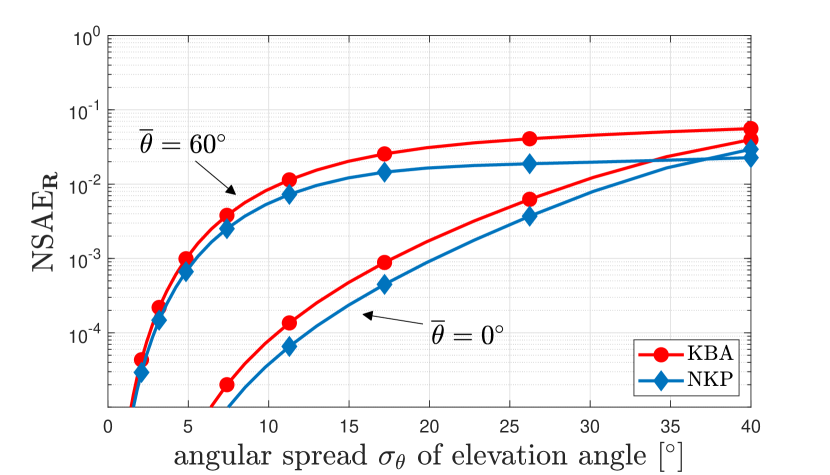
(a) $\mathsf{NSAE}_{\mathbf{R}}$ in (29).

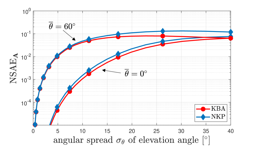
(b) $\mathsf{NSAE}_{\mathbf{A}}$ in (31).

Figure 2: NSAE of the correlation matrix as a function of the elevation angular spread for KBA and NKP. We consider a UPA with $N_{\mathsf{H}}=N_{\mathsf{V}}=16$ elements, using $\Delta_{\mathsf{H}}=\Delta_{\mathsf{V}}=\lambda/4$ at $3\,\mathrm{GHz}$. The azimuth angle is $\overline{\varphi}=0^{\circ}$ with angular spread $\sigma_{\varphi}=10^{\circ}$. Both azimuth and elevation angles follow a Gaussian distribution.

In Figure 2(a), comparisons are made with the nearest Kronecker product (NKP), derived in [20] by minimizing the NSAE. According to NKP, the matrix $\boldsymbol{\mathbf{R}}_{k}$ is approximated by $\boldsymbol{\mathbf{R}}^{\star}_{\mathsf{V},k}\otimes\boldsymbol{\mathbf{R}}^{\star}_{\mathsf{H},k}$, where $\boldsymbol{\mathbf{R}}^{\star}_{\mathsf{H},k}$ and $\boldsymbol{\mathbf{R}}^{\star}_{\mathsf{V},k}$ are obtained as

$$\left(\boldsymbol{\mathbf{R}}^{\star}_{\mathsf{H},k},\boldsymbol{\mathbf{R}}^{\star}_{\mathsf{V},k}\right)=\arg\underset{\left(\boldsymbol{\mathbf{X}},\boldsymbol{\mathbf{Y}}\right)}{\min}\left\|\boldsymbol{\mathbf{R}}_{k}-\boldsymbol{\mathbf{Y}}\otimes\boldsymbol{\mathbf{X}}\right\|^{2}_{\mathsf{F}}.$$ (30)

The NKP solution can be found following the steps detailed in [21]. From Figure 2(a), we see that difference between NKP and KBA is relatively small for all the considered values of $\sigma_{\theta}$. Notice that, despite (30) is the solution that best approximates $\boldsymbol{\mathbf{R}}_{k}$, KBA performs better than NKP as far as the approximation of $\boldsymbol{\mathbf{A}}^{\mathsf{MMSE}}_{k}$ in (9) is concerned. This can be appreciated with the help of Figure 2(b), which reports

$$\mathsf{NSAE}_{\mathbf{A}}=\frac{\left\|\boldsymbol{\mathbf{A}}^{\mathsf{MMSE}}_{k}-\boldsymbol{\mathbf{A}}_{k}\right\|^{2}_{\mathsf{F}}}{\|\boldsymbol{\mathbf{A}}^{\mathsf{MMSE}}_{k}\|^{2}_{\mathsf{F}}}$$ (31)

as a function of $\sigma_{\theta}$ for $\gamma=10\,\mathrm{dB}$. The matrix $\boldsymbol{\mathbf{A}}_{k}$ in (31) is obtained from (9) by replacing $\boldsymbol{\mathbf{R}}_{k}$ with either $\boldsymbol{\mathbf{R}}_{\mathsf{V},k}\otimes\boldsymbol{\mathbf{R}}_{\mathsf{H},k}$ (KBA curves) or $\boldsymbol{\mathbf{R}}^{\star}_{\mathsf{V},k}\otimes\boldsymbol{\mathbf{R}}^{\star}_{\mathsf{H},k}$ (NKP curves). We see that KBA yields a lower $\mathsf{NSAE}_{\mathbf{A}}$, which results in a superior estimation accuracy when implementing (6), as shown next.

IV-B NMSE evaluation

Consider a square UPA with $N_{\mathsf{H}}=N_{\mathsf{V}}=\sqrt{N}$ and all the other relevant parameters listed in Table I. Figure 3 shows the NMSE in (7) as a function of $N=N_{\mathsf{H}}N_{\mathsf{V}}$. The matrix $\boldsymbol{\mathbf{A}}_{k}$ in (7) depends on the specific channel estimation scheme. We consider: MMSE, LS, LoS, ISO, and the approximate MMSE based on KBA. We evaluate the average NMSE for a UE randomly placed in the simulation setup detailed in Table II, in which the received SNR is $\beta_{k}\tau_{p}\rho/\sigma^{2}$. The path loss $\beta_{k}$ is computed following [2, Sect. 2], i.e.,

$$\beta_{k}=-148.1\,\mathrm{dB}-37.6\log_{10}\left(\frac{d_{k}}{1\,\mathrm{km}}\right)\qquad\textrm{[dB]}$$ (32)

where $d_{k}$ is the distance of UE $k$. The results of Figure 3 show that the accuracy of the KBA-based estimator attains that of the optimal MMSE, irrespective of the size $N$. This happens despite the error in the approximation of $\boldsymbol{\mathbf{R}}_{k}$. The accuracy of the NKP-based estimator, not reported in Figure 3, overlaps both the MMSE and the KBA ones. Similar results can be obtained with a UPA with a rectangular shape.

Table I: UPA parameters.

Parameter	Value
Carrier frequency	$f_{0}=3\,\mathrm{GHz}$
Wavelength	$\lambda=10\,\mathrm{cm}$
Vertical inter-element spacing	$\Delta_{\mathsf{V}}=\lambda/4=2.5\,\mathrm{cm}$
Horizontal inter-element spacing	$\Delta_{\mathsf{H}}=\lambda/4=2.5\,\mathrm{cm}$
Height	$b=10\,\mathrm{m}$

Table II: Simulation parameters.

Parameter	Value
Minimum distance from UPA $\underline{d}$	$5\,\mathrm{m}$
Maximum distance from UPA $\overline{d}$	$100\,\mathrm{m}$
Azimuth range $\varphi$	$\left[-60^{\circ},+60^{\circ}\right]$
Azimuth spreading $\sigma_{\varphi}$	$10^{\circ}$
Elevation range $\theta$	$\left[-63.4^{\circ},-5.7^{\circ}\right]$
Elevation spreading $\sigma_{\theta}$	$10^{\circ}$
Azimuth/elevation scattering distribution	Gaussian
Path loss reference distance	$1\,\mathrm{km}$
Channel gain at reference distance	$-148.1\,\mathrm{dB}$
Path loss exponent	$3.76$
Communication bandwidth $B$	$100\,\mathrm{MHz}$
Transmit power $\rho$	$20\,\mathrm{dBm}$
Noise power	$-87\,\mathrm{dBm}$
Length of pilot sequence $\tau_{p}$	$10$
Length of coherence block $\tau_{c}$	$200$

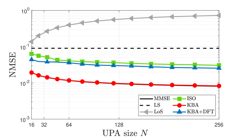
Figure 3: NMSE for a square UPA with $N_{\mathsf{H}}=N_{\mathsf{V}}=\sqrt{N}$. The UPA parameters are reported in Table I. The simulation parameters are those of Table II.

Figure 4: Average NMSE as a function of the angular spread $\sigma_{\theta}$ of the elevation angle for the UPA with parameters reported in Table I and $N_{\mathsf{H}}=N_{\mathsf{V}}=16$. The simulation parameters are those of Table II.

The impact of the angular spread $\sigma_{\theta}$ is evaluated in Figure 4. The same simulation setup of Figure 3 is considered. Also, we assume $N_{\mathsf{H}}=N_{\mathsf{V}}=16$ and set $\sigma_{\varphi}=10^{\circ}$. The results show that the KBA-based estimator achieves the best accuracy. For $10^{\circ}\leq\sigma_{\theta}\leq 40^{\circ}$, the difference between KBA and NKP increases, thus confirming the findings of Figure 2.

Sect. V Reduced-complexity methods for ULA

The UPA model introduced in Sect. II is general enough to encompass both vertical and horizontal configurations, obtained by either $N_{\mathsf{H}}=1$ or $N_{\mathsf{V}}=1$, respectively. In those cases, the KBA-based approach has exactly the same complexity of the optimal MMSE one. This is due to the fact that, when $N_{\mathsf{H}}$ (respectively, $N_{\mathsf{V}}$) is equal to $1$, based on (27) [respectively, (28)], the matrix $\boldsymbol{\mathbf{R}}_{\mathsf{H},k}(\overline{\theta})$ [respectively, $\boldsymbol{\mathbf{R}}_{\mathsf{V},k}(\overline{\theta})$] is exactly the scalar $1$, and hence $\boldsymbol{\mathbf{R}}_{k}=\boldsymbol{\mathbf{R}}_{\mathsf{V},k}(\overline{\theta})$ [respectively, $\boldsymbol{\mathbf{R}}_{k}=\boldsymbol{\mathbf{R}}_{\mathsf{H},k}(\overline{\theta})$]. For this reason, not only the complexity, but also the channel estimation performance of the KBA-based method coincides with the MMSE one.

In this section, we develop a channel estimation scheme for a horizontal ULA (i.e., $N=N_{\mathsf{H}}$) that exploits the correlation induced by the array geometry and propagation conditions to approach MMSE performance, while having a computational complexity that scales log-linearly with $N$. The adaptation to the vertical ULA configuration (with $N=N_{\mathsf{V}}$) is straightforward and not reported here for the sake of brevity.

V-A DFT-based approximation

If a ULA is used, the covariance matrix $\boldsymbol{\mathbf{R}}_{k}$ is Hermitian Toeplitz, and it can be approximated with a suitable circulant matrix $\boldsymbol{\mathbf{C}}_{k}$ [22, 23, 24], whose first row $\boldsymbol{\mathbf{c}}_{k}=[c_{k}(0),c_{k}(1),\cdots,c_{k}(N-1)]$ is related to the first row $\boldsymbol{\mathbf{r}}_{k}=[r_{k}(0),r_{k}(1),\cdots,r_{k}(N-1)]$ of $\boldsymbol{\mathbf{R}}_{k}$ by [24]

$$c_{k}(n)=\begin{cases}r_{k}(0)&\text{$n=0$},\\ \dfrac{(N-n)r_{k}(n)+nr^{*}_{k}(N-n)}{N}&\text{$n=1,\ldots,N-1$}.\end{cases}$$ (33)

Any circulant matrix can be unitarily diagonalized using the discrete Fourier transform (DFT) matrix, i.e., ${\boldsymbol{\mathbf{C}}}_{k}={\boldsymbol{\mathbf{F}}}{\boldsymbol{\mathbf{\Lambda}}}_{k}{\boldsymbol{\mathbf{F}}}^{\mathsf{H}}$ where ${\boldsymbol{\mathbf{F}}}=[{\boldsymbol{\mathbf{f}}}_{0}\,{\boldsymbol{\mathbf{f}}}_{1}\,\cdots\,{\boldsymbol{\mathbf{f}}}_{N-1}]$ is the inverse DFT matrix, with $[{\boldsymbol{\mathbf{f}}}_{n}]_{m}=\frac{1}{\sqrt{N}}e^{\mathsf{j}2\pi mn/N}$ for $0\leq m,n\leq N-1$, and ${\boldsymbol{\mathbf{\Lambda}}}_{k}$ is the diagonal matrix containing the eigenvalues of ${\boldsymbol{\mathbf{C}}}_{k}$, i.e.,

$$[{\boldsymbol{\mathbf{\Lambda}}}_{k}]_{n,n}=\sum\limits_{m=0}^{N-1}c_{k}(m)e^{-\mathsf{j}2\pi mn/N}$$ (34)

which are obtained by taking the DFT of the first row of $\boldsymbol{\mathbf{C}}_{k}$. Replacing $\boldsymbol{\mathbf{R}}_{k}$ with $\boldsymbol{\mathbf{C}}_{k}$ into (9) yields $\widehat{\boldsymbol{\mathbf{h}}}_{k}^{\mathsf{DFT}}={\bf A}_{k}^{\mathsf{DFT}}\boldsymbol{\mathbf{y}}_{k}$, with

$$\boldsymbol{\mathbf{A}}_{k}^{\mathsf{DFT}}=\frac{1}{\tau_{p}\sqrt{\rho}}{\boldsymbol{\mathbf{F}}}\,{\boldsymbol{\mathbf{\Lambda}}_{k}}\left({\boldsymbol{\mathbf{\Lambda}}_{k}}+\frac{1}{\gamma}{\boldsymbol{\mathbf{I}}}_{N}\right)^{-1}{\boldsymbol{\mathbf{F}}}^{\mathsf{H}}.$$ (35)

We call it the DFT-based channel estimator. Its complexity derives from the pre-computation phase, which is $\mathcal{O}(N\log N)$ due to the computation of ${\boldsymbol{\mathbf{\Lambda}}}_{k}$ through (34), and from the computation of the matrix-vector product, which is again $\mathcal{O}(N\log N)$, since the DFT matrix $\boldsymbol{\mathbf{F}}$ and its inverse are involved. Hence, the complexity of the DFT-based estimator is $\mathcal{C}_{\mathsf{DFT}}=\mathcal{O}(N\log N)$. Note that, similarly to the KBA case, the DFT-based estimator depends on the true covariance matrix ${\boldsymbol{\mathbf{R}}}_{k}$, which must be estimated as with the MMSE estimator.

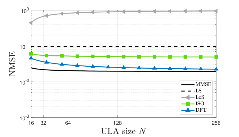
Figure 5: NMSE as a function of the ULA size $N$.

V-B NMSE analysis

Consider a horizontal ULA, using the relevant parameters listed in Tables I and II. Figure 5 shows the NMSE in (7) as a function of $N$. We see that the accuracy of the DFT-based estimator is comparable with the MMSE, and the difference decreases as $N$ increases. This is due to the fact that the circulant approximation $\boldsymbol{\mathbf{C}}_{k}$ of the covariance matrix $\boldsymbol{\mathbf{R}}_{k}$ improves as $N$ grows. Interestingly, the circulant approximation is already quite tight for $N=64$ (which means $L=N\Delta_{\mathsf{H}}=1.6\,\mathrm{m}$). More importantly, this is obtained with a complexity of $\mathcal{O}(N\log N)$, instead of $\mathcal{O}(N^{3})$. If $N=64$, this corresponds to two orders of magnitude of computational saving compared to MMSE. Please refer to [1] for numerical results of vertical ULAs in terms of performance as a function of the ULA size and of the angular spreads.

V-C The failure of the combination with KBA

Inspired by the circulant approximation that exploits the Toeplitz structure of $\boldsymbol{\mathbf{R}}_{k}$ in a ULA, one might be tempted to adopt the same approach for the matrices $\boldsymbol{\mathbf{R}}_{\mathsf{H},k}$ and $\boldsymbol{\mathbf{R}}_{\mathsf{V},k}$ in (24) since as they are both Hermitian Toeplitz. This means applying (33) to the first row of either matrix $\boldsymbol{\mathbf{R}}_{\mathsf{H},k}$ or $\boldsymbol{\mathbf{R}}_{\mathsf{V},k}$.

Unfortunately, since the covariance matrix $\boldsymbol{\mathbf{R}}_{k}$ in a UPA is Hermitian block-Toeplitz (and not simply Toeplitz), this approach does not yield the sufficient accuracy. To showcase this, Figure 6 illustrates the NSAE as a function of $\sigma_{\theta}$ for the following configurations: $(N_{\mathsf{H}}=N_{\mathsf{V}}=16)$ (solid lines), $(N_{\mathsf{H}}=1,N_{\mathsf{V}}=256)$ (dashed lines), and $(N_{\mathsf{H}}=4,N_{\mathsf{V}}=64)$ (dotted lines). We consider $\overline{\varphi}=\overline{\theta}=0^{\circ}$, and the scattering of both angles is modeled as Gaussian, with $\sigma_{\theta}=\sigma_{\varphi}=10^{\circ}$. Red lines with circular markers represent the results by combining the KBA and DFT approaches described above, whereas blue lines with diamond markers report the NKP solution introduced in Sect. IV-A. As can be seen, keeping the UPA size $N$ constant, the performance gap for all configurations is significant, especially for moderate values of $\sigma_{\theta}$, which are of particular interest in practical working conditions.

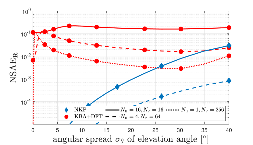
Figure 6: NSAE of the correlation matrix as a function of the elevation spreading for the combined KBA/DFT approach and the NKP solution.

The impact in terms of channel estimation accuracy can be seen in Figure 3 (blue curve), which confirms the poor accuracy achieved by the KBA/DFT combined method – the accuracy is significantly worse than that achieved by the KBA estimator.

Sect. VI Channel estimation with imperfect knowledge of covariance matrices

So far, we have assumed perfect knowledge of $\boldsymbol{\mathbf{R}}_{k}$. This may not be the case in practical scenarios since $\boldsymbol{\mathbf{R}}_{k}$ changes for various reasons [4]. Measurements suggest about orders of magnitude slower than the fast variations of the channel vectors. Therefore, it is reasonable to assume that they do not change over $\tau_{s}$ coherence blocks, where $\tau_{s}$ can be on the order of thousands [4]. Suppose the BS has the pilot symbols $\boldsymbol{\mathbf{\phi}}_{k}$ in $M\leq\tau_{s}$ coherence blocks. We denote the corresponding observations by $\boldsymbol{\mathbf{y}}_{k}[1],\ldots,\boldsymbol{\mathbf{y}}_{k}[M]$. An estimate of ${\boldsymbol{\mathbf{Q}}}_{k}$ can be obtained by computing the sample correlation matrix given by

$$\widehat{\boldsymbol{\mathbf{Q}}}_{k}^{\mathsf{sample}}=\frac{1}{M}\sum_{m=1}^{M}\frac{\boldsymbol{\mathbf{y}}_{k}[m]\boldsymbol{\mathbf{y}}_{k}^{\mathsf{H}}[m]}{\rho\tau_{p}^{2}}.$$ (36)

The computation of $\widehat{\boldsymbol{\mathbf{Q}}}_{k}^{\mathsf{sample}}$ requires $\mathcal{O}(MN^{2})$ operations, as it involves $MN^{2}$ complex multiplications.

A better estimation is typically obtained through matrix regularization by computing the convex combination [4]:

$$\widehat{\boldsymbol{\mathbf{Q}}}_{k}(\eta)=\eta\widehat{\boldsymbol{\mathbf{Q}}}_{k}^{\mathsf{sample}}+(1-\eta)\widehat{\boldsymbol{\mathbf{Q}}}_{k}^{\mathsf{diag}},\quad\eta\in[0,1]$$ (37)

where $\widehat{\boldsymbol{\mathbf{Q}}}_{k}^{\mathsf{diag}}$ contains the main diagonal of $\widehat{\boldsymbol{\mathbf{Q}}}_{k}^{\mathsf{sample}}$. The regularization makes $\widehat{\boldsymbol{\mathbf{Q}}}_{k}(\eta)$ a full-rank matrix for any $\eta\in[0,1)$, and $\eta$ can be tuned (for example by using numerical methods) to purposely underestimate the off-diagonal elements when these are considered unreliable. Once $\widehat{\boldsymbol{\mathbf{Q}}}_{k}(\eta)$ is computed, an estimate of ${\boldsymbol{\mathbf{R}}}_{k}$ follows:

$$\widehat{\boldsymbol{\mathbf{R}}}_{k}(\eta)=\widehat{\boldsymbol{\mathbf{Q}}}_{k}(\eta)-\frac{1}{\gamma}{\boldsymbol{\mathbf{I}}}_{N}$$ (38)

which requires only knowledge of $\gamma$, i.e., the SNR during the pilot transmission phase.

VI-A Improved estimation of ${\boldsymbol{\mathbf{Q}}}_{k}$ and ${\boldsymbol{\mathbf{R}}}_{k}$

We now develop an improved estimation scheme of the correlation matrix $\boldsymbol{\mathbf{Q}}_{k}$ that can be used with UPAs. For the ease of notation, we will drop the subscript $k$ from now on.

To accomplish this task, we notice that $\boldsymbol{\mathbf{Q}}$ is Hermitian block-Toeplitz with $N_{\mathsf{V}}\times N_{\mathsf{V}}$ blocks with size $N_{\mathsf{H}}\times N_{\mathsf{H}}$, i.e.,

$$\boldsymbol{\mathbf{Q}}=\begin{bmatrix}\boldsymbol{\mathbf{Q}}_{1,1}&\boldsymbol{\mathbf{Q}}_{1,2}&\boldsymbol{\mathbf{Q}}_{1,3}&\ldots&\boldsymbol{\mathbf{Q}}_{1,N_{\mathsf{V}}}\\ \boldsymbol{\mathbf{Q}}_{1,2}^{\mathsf{H}}&\boldsymbol{\mathbf{Q}}_{1,1}&\boldsymbol{\mathbf{Q}}_{1,2}&\ldots&\boldsymbol{\mathbf{Q}}_{1,N_{\mathsf{V}}-1}\\ \boldsymbol{\mathbf{Q}}_{1,3}^{\mathsf{H}}&\boldsymbol{\mathbf{Q}}_{1,2}^{\mathsf{H}}&\boldsymbol{\mathbf{Q}}_{1,1}&\ldots&\boldsymbol{\mathbf{Q}}_{1,N_{\mathsf{V}}-2}\\ \vdots&\vdots&\vdots&\ddots&\vdots\\ \boldsymbol{\mathbf{Q}}_{1,N_{\mathsf{V}}}^{\mathsf{H}}&\boldsymbol{\mathbf{Q}}_{1,N_{\mathsf{V}}-1}^{\mathsf{H}}&\boldsymbol{\mathbf{Q}}_{1,N_{\mathsf{V}}-2}^{\mathsf{H}}&\ldots&\boldsymbol{\mathbf{Q}}_{1,1}\end{bmatrix},$$ (39)

where $\boldsymbol{\mathbf{Q}}_{1,j}$ denotes the $N_{\mathsf{H}}\times N_{\mathsf{H}}$ block obtained by $\boldsymbol{\mathbf{Q}}$ as (using MatLab colon notation)

$$\boldsymbol{\mathbf{Q}}_{1,j}=\left[\boldsymbol{\mathbf{Q}}\right]_{1:1:N_{\mathsf{H}},\left(j-1\right)N_{\mathsf{H}}+1:1:jN_{\mathsf{H}}}.$$ (40)

This means that, due to the block-Toeplitz structure,

$$\boldsymbol{\mathbf{Q}}_{1+m,j+m}=\boldsymbol{\mathbf{Q}}_{1,j}$$ (41)

for $j=1,\dots,N_{\mathsf{V}}-1$ and $m=1,\dots,N_{\mathsf{V}}-j$, and that

$$\boldsymbol{\mathbf{Q}}_{j,1}=\boldsymbol{\mathbf{Q}}_{1,j}^{\mathsf{H}},$$ (42)

because of the Hermitian symmetry of the covariance matrix.

To proceed with the estimation, we denote by $\widehat{\boldsymbol{\mathbf{Q}}}_{1,j}$ the estimate of $\boldsymbol{\mathbf{Q}}_{1,j}$ that takes the block-Toeplitz structure (39) into account, i.e., by averaging the blocks of $\widehat{\boldsymbol{\mathbf{Q}}}^{\mathsf{sample}}$ over the same (block) diagonal:

$$\widehat{\boldsymbol{\mathbf{Q}}}_{1,j}=\frac{1}{N_{\mathsf{V}}-j+1}\sum_{m=1}^{N_{\mathsf{V}}-j+1}{\widehat{\boldsymbol{\mathbf{Q}}}^{\mathsf{sample}}_{m,j+m-1}},$$ (43)

for $j=1,\dots,N_{\mathsf{V}}$, where ${\widehat{\boldsymbol{\mathbf{Q}}}^{\mathsf{sample}}_{m,j+m-1}}$ is the $N_{\mathsf{H}}\times N_{\mathsf{H}}$ block corresponding to the rows $(m-1)N_{\mathsf{H}}+1,\ldots,mN_{\mathsf{H}}-1$ and to the columns $(j+m-2)N_{\mathsf{H}}+1,\ldots,(j+m-1)N_{\mathsf{H}}-1$ of $\widehat{\boldsymbol{\mathbf{Q}}}^{\mathsf{sample}}$ in (36).

It is worth noting that $\boldsymbol{\mathbf{Q}}_{1,j}$ is an $N_{\mathsf{H}}\times N_{\mathsf{H}}$ Toeplitz (but not Hermitian) matrix, and we can thus improve the estimation further, by adapting the matrix-based criterion (43) to the elements of $\boldsymbol{\mathbf{Q}}_{1,j}$. In particular, the estimate ${\widehat{\boldsymbol{\mathbf{Q}}}^{\mathsf{toe}}_{1,j}}$ can be obtained as follows: the first row is computed as

$$\left[\widehat{\boldsymbol{\mathbf{Q}}}^{\mathsf{toe}}_{1,j}\right]_{1,\ell}=\frac{1}{N_{\mathsf{H}}-\ell+1}\sum_{m=1}^{N_{\mathsf{H}}-\ell+1}{\left[\widehat{\boldsymbol{\mathbf{Q}}}_{1,j}\right]_{m,\ell+m-1}}$$ (44)

for $\ell=1,\dots,N_{\mathsf{H}}$, whereas the first column can be computed as

$$\left[\widehat{\boldsymbol{\mathbf{Q}}}^{\mathsf{toe}}_{1,j}\right]_{\ell,1}=\frac{1}{N_{\mathsf{H}}-\ell+1}\sum_{m=1}^{N_{\mathsf{H}}-\ell+1}{\left[\widehat{\boldsymbol{\mathbf{Q}}}_{1,j}\right]_{\ell+m-1,m}}$$ (45)

for $\ell=1,\dots,N_{\mathsf{H}}$. Exploiting the Toeplitz structure, the remaining elements of $\widehat{\boldsymbol{\mathbf{Q}}}^{\mathsf{toe}}_{i,j}$ can be found as

$$\left[\widehat{\boldsymbol{\mathbf{Q}}}^{\mathsf{toe}}_{1,j}\right]_{1+m,\ell+m} =\left[\widehat{\boldsymbol{\mathbf{Q}}}^{\mathsf{toe}}_{1,j}\right]_{1,\ell}$$ (46)

$$\left[\widehat{\boldsymbol{\mathbf{Q}}}^{\mathsf{toe}}_{1,j}\right]_{\ell+m,1+m} =\left[\widehat{\boldsymbol{\mathbf{Q}}}^{\mathsf{toe}}_{1,j}\right]_{\ell,1}$$ (47)

for $\ell=1,\dots,N_{\mathsf{H}}-1$ and $m=1,\dots,N_{\mathsf{H}}-\ell$.

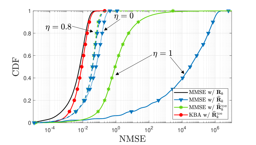
Figure 7: CDF of the NMSE as a function of the estimation technique using $M=50$ (black: MMSE with perfect knowledge of $\boldsymbol{\mathbf{R}}_{k}$; red: KBA using $\widehat{\boldsymbol{\mathbf{R}}}^{\mathsf{toe}}_{k}$ (48); blue: MMSE using $\widehat{\boldsymbol{\mathbf{R}}}_{k}(\eta)$ (38) in (9) as a function of $\eta$; green: MMSE using $\widehat{\boldsymbol{\mathbf{R}}}^{\mathsf{toe}}_{k}(\eta)$ (48) in (9) as a function of $\eta$).

Once $\boldsymbol{\mathbf{Q}}_{1,j}$ is available for $j=1,...,N_{\mathsf{V}}$, the estimate $\widehat{\boldsymbol{\mathbf{Q}}}^{\mathsf{toe}}$ of the covariance matrix $\boldsymbol{\mathbf{Q}}$ can be found by the same structure as in (39), using $\widehat{\boldsymbol{\mathbf{Q}}}^{\mathsf{toe}}_{1,j}$ instead of ${\boldsymbol{\mathbf{Q}}}_{1,j}$. An estimate of $\boldsymbol{\mathbf{R}}$ is finally obtained as

$$\widehat{\boldsymbol{\mathbf{R}}}^{\mathsf{toe}}=\widehat{\boldsymbol{\mathbf{Q}}}^{\mathsf{toe}}-\frac{\boldsymbol{\mathbf{I}}_{N}}{\gamma}.$$ (48)

The complexity of the estimator above is mainly due to the computation of $\widehat{\boldsymbol{\mathbf{Q}}}^{\mathsf{sample}}$, and thus is comparable to the one not exploiting the Toeplitz structure, as shown in Sect. VII.

To implement the MMSE estimation scheme, we can replace $\boldsymbol{\mathbf{R}}$ and $\boldsymbol{\mathbf{Q}}$ in (9) with $\widehat{\boldsymbol{\mathbf{R}}}^{\mathsf{toe}}$ and $\widehat{\boldsymbol{\mathbf{Q}}}^{\mathsf{toe}}$, respectively. We can also adopt the KBA- and the DFT-based methods, for the UPA and ULA cases, respectively, by considering $\widehat{\boldsymbol{\mathbf{R}}}^{\mathsf{toe}}$ in (24) and (33), instead of $\boldsymbol{\mathbf{R}}$.

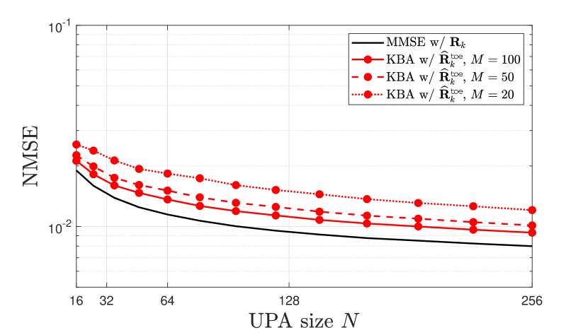
Figure 8: NMSE as a function of the size $N$ (square UPA, with $N_{\mathsf{H}}=N_{\mathsf{V}}$) with imperfect statistical knowledge (KBA-based estimator).

VI-B Performance analysis

We now evaluate the accuracy of the different estimators, using the system setup detailed in Table II, assuming a square UPA with parameters listed in Table I. Figure 7 reports the cumulative distribution function (CDF) of NMSE in (7) asssuming that $M=50$ observations are used for the estimation of the channel covariance matrix. In particular, the red line with circular markers corresponds to the KBA estimator that uses $\widehat{\boldsymbol{\mathbf{R}}}^{\mathsf{toe}}_{k}$ in (48), whereas blue and green lines correspond to the MMSE estimator when using (38) and (48), respectively. Solid, dashed, and dotted lines report the results obtained with the regularization parameter $\eta$ introduced in (37) with values $\{1,0.8,0\}$, respectively. For comparison, we also report the NMSE achieved by the MMSE estimator with perfect knowledge of $\boldsymbol{\mathbf{R}}_{k}$ (black line).

The KBA estimator performs close to the MMSE estimator with perfect knowledge of channel statistics, whereas the MMSE estimator with imperfect knowledge of channel statistics shows a gap that depends on $\eta$, and thus confirming the benefits yielded by the regularization technique (37). Note also that the MMSE estimator using (48) outperforms the one using (38). For this reason, in the remainder of the paper, we will adopt (48) with a regularization factor $\eta=0.8$. Additional simulations, not reported for the sake of clarity, show that: i) regularizing the KBA estimator does not provide additional benefits, as the performance is already tight to the optimal one; and ii) using (38) instead of (48) produces poorer performance of the KBA estimator. Hence, in the remainder of the paper we will use (48) when considering KBA.

Figure 8 reports the average as a function of the size $N$ for a square UPA, obtained by averaging over all possible UE positions in the system setup detailed in Table II. As can be seen, an estimation accuracy comparable to that obtained with perfect knowledge of $\boldsymbol{\mathbf{R}}_{k}$ is already achieved with $M=20$. Similar trends are observed for different array sizes and/or scattering scenarios. The results concerning ULA configurations are reported in [1].

Sect. VII Complexity analysis

Next, we assess the computational burden in terms of complex operations (additions and/or multiplications), required by the entire channel estimation procedure of the investigated estimators. Without loss of generality, next we consider $N_{\mathsf{H}}\geq N_{\mathsf{V}}$. The analysis can be simply extended to the case $N_{\mathsf{H}}<N_{\mathsf{V}}$.

VII-A Computation of ${\widehat{\boldsymbol{\mathbf{Q}}}_{k}^{\mathsf{toe}}}$

From (43), the calculation of $\widehat{\boldsymbol{\mathbf{Q}}}_{1,j}$, for $j=1,\dots,N_{\mathsf{V}}$, requires a total of approximately $N^{2}/2$ additions and $N_{\mathsf{H}}N$ multiplications. Analogously, the evaluation of ${\widehat{\boldsymbol{\mathbf{Q}}}^{\mathsf{toe}}_{1,j}}$ in (44), with $j=1,\dots,N_{\mathsf{V}}$, requires a total of $NN_{\mathsf{H}}/2$ additions and $N$ multiplications. Thanks to Toeplitz-block Toeplitz structure, the computation of ${\widehat{\boldsymbol{\mathbf{Q}}}_{k}^{\mathsf{toe}}}$ has a complexity order of $\mathcal{O}(MN^{2}+N^{2}/2+N_{\mathsf{H}}N)\approx\mathcal{O}(MN^{2})$. No additional complexity is incurred compared to the unstructured $\widehat{\boldsymbol{\mathbf{Q}}}_{k}^{\mathsf{sample}}$.

VII-B Computation of matrix $\boldsymbol{\mathbf{A}}_{k}$ via ${\widehat{\boldsymbol{\mathbf{R}}}_{k}^{\mathsf{toe}}}$ and ${\widehat{\boldsymbol{\mathbf{Q}}}_{k}^{\mathsf{toe}}}$

The MMSE estimator is characterized by the matrix

$$\widehat{\boldsymbol{\mathbf{A}}}_{k}^{\mathsf{MMSE}}=\frac{1}{\tau_{p}\sqrt{\rho}}{\widehat{\boldsymbol{\mathbf{R}}}}^{\mathsf{toe}}_{k}\left(\widehat{\boldsymbol{\mathbf{Q}}}_{k}^{\mathsf{toe}}\right)^{-1}$$ (49)

obtained from (9) by replacing the true covariance matrix $\boldsymbol{\mathbf{R}}_{k}$ with its estimate $\widehat{\boldsymbol{\mathbf{R}}}^{\mathsf{toe}}_{k}$. Once ${\widehat{\boldsymbol{\mathbf{Q}}}_{k}^{\mathsf{toe}}}$ is available, $\widehat{\boldsymbol{\mathbf{R}}}^{\mathsf{toe}}_{k}$ can easily be obtained through (48) with $N$ additions. As for the computation of $(\widehat{\boldsymbol{\mathbf{Q}}}^{\mathsf{toe}}_{k})^{-1}$, an efficient algorithm for the inversion of a Toeplitz-block Toeplitz matrix can be found in [28]. It has a complexity $\mathcal{O}(N^{2}N_{\mathsf{V}})$. The maximum complexity occurs for square UPAs, where $N_{\mathsf{H}}=N_{\mathsf{V}}=\sqrt{N}$, resulting in $\mathcal{O}(N^{2.5})$.

Table III: Complexity of channel estimation schemes.

Scheme	${\widehat{\boldsymbol{\mathbf{Q}}}^{\mathsf{toe}}}$	$\boldsymbol{\mathbf{A}}_{k}$	$\boldsymbol{\mathbf{A}}_{k}\boldsymbol{\mathbf{y}}_{k}$
LS	–	–	$\mathcal{O}(N)$
LoS	–	–	$\mathcal{O}(N)$
ISO	–	–	$\mathcal{O}(N^{2})$
MMSE	$\mathcal{O}(MN^{2})$	$\mathcal{O}(N^{2}N_{\mathsf{V}})$	$\mathcal{O}(N^{2})$
KBA	$\mathcal{O}(MN^{2})$	$\mathcal{O}(N_{\mathsf{H}}^{3})$	$\mathcal{O}((N_{\mathsf{H}}+N_{\mathsf{V}})N)$
DFT	$\mathcal{O}(N^{2})$	$\mathcal{O}(N\log N)$	$\mathcal{O}(N\log N)$

The KBA estimator is obtained by approximating $\widehat{\boldsymbol{\mathbf{R}}}_{k}^{\mathsf{toe}}$ with the Kronecker product $\widehat{\boldsymbol{\mathbf{R}}}^{\mathsf{toe}}_{\mathsf{V},k}\otimes\widehat{\boldsymbol{\mathbf{R}}}^{\mathsf{toe}}_{\mathsf{H},k}$. The matrix $\widehat{\boldsymbol{\mathbf{A}}}_{k}^{\mathsf{KBA}}$ is derived from (IV) by replacing

$${\boldsymbol{\mathbf{K}}}_{1} =\boldsymbol{\mathbf{U}}_{1}\boldsymbol{\mathbf{\Lambda}}_{1}\boldsymbol{\mathbf{U}}_{1}^{\mathsf{H}}$$ (50)

$${\boldsymbol{\mathbf{K}}}_{2} =\boldsymbol{\mathbf{U}}_{2}\boldsymbol{\mathbf{\Lambda}}_{2}\boldsymbol{\mathbf{U}}_{2}^{\mathsf{H}}$$ (51)

with

$$\widehat{\boldsymbol{\mathbf{R}}}^{\mathsf{toe}}_{\mathsf{V},k} =\widehat{\boldsymbol{\mathbf{U}}}_{\mathsf{V},k}^{\mathsf{toe}}\widehat{\boldsymbol{\mathbf{\Lambda}}}_{\mathsf{V},k}^{\mathsf{toe}}(\widehat{\boldsymbol{\mathbf{U}}}_{\mathsf{V},k}^{\mathsf{toe}})^{\mathsf{H}}$$ (52)

$$\widehat{\boldsymbol{\mathbf{R}}}^{\mathsf{toe}}_{\mathsf{H},k} =\widehat{\boldsymbol{\mathbf{U}}}_{\mathsf{H},k}^{\mathsf{toe}}\widehat{\boldsymbol{\mathbf{\Lambda}}}_{\mathsf{H},k}^{\mathsf{toe}}(\widehat{\boldsymbol{\mathbf{U}}}_{\mathsf{H},k}^{\mathsf{toe}})^{\mathsf{H}}$$ (53)

respectively. By utilizing the algorithm proposed in [29], the computation of (52) and (53) has a complexity of $\mathcal{O}(N_{\mathsf{H}}^{3})$ and $\mathcal{O}(N_{\mathsf{V}}^{3})$, respectively. Consequently, the factorization of $\widehat{\boldsymbol{\mathbf{A}}}_{k}^{\mathsf{KBA}}$ can be achieved with a complexity of $\mathcal{O}(N_{\mathsf{H}}^{3})$, which amounts to $\mathcal{O}(N^{1.5})$ for square UPAs.

VII-C Computation of channel estimate $\widehat{\boldsymbol{\mathbf{h}}}_{k}$

All estimation schemes are linear of the form given in (6), based on $\boldsymbol{\mathbf{y}}_{k}$. The complexity associated with the computation of $\boldsymbol{\mathbf{y}}_{k}$ is $\mathcal{O}(N)$, since it requires $(\tau_{p}-1)N$ complex sums and $\tau_{p}N$ complex products.

The LS estimator simply multiplies $\boldsymbol{\mathbf{y}}_{k}$ and the real diagonal matrix in (11). Accordingly, it has an overall complexity $\mathcal{O}(N)$. The MMSE estimator multiplies $\boldsymbol{\mathbf{y}}_{k}$ by the matrix (49). From the Appendix, it follows that it exhibits a computational complexity of $\mathcal{O}(N^{2})$. This is because computing $(\widehat{\boldsymbol{\mathbf{Q}}}_{k}^{\mathsf{toe}})^{-1}\boldsymbol{\mathbf{y}}_{k}$ requires $N^{2}$ multiplications and (approximately) $N^{2}$ additions, and the same number of operations is needed to compute $\widehat{\boldsymbol{\mathbf{R}}}_{k}^{\mathsf{toe}}(\widehat{\boldsymbol{\mathbf{Q}}}_{k}^{\mathsf{toe}})^{-1}\boldsymbol{\mathbf{y}}_{k}$.

The KBA scheme makes use of the matrix $\widehat{\boldsymbol{\mathbf{A}}}_{k}^{\mathsf{KBA}}$. From the Appendix, based on (IV) and exploiting the structure of KBA due to the Kronecker products, the complexity associated with the computation of $\widehat{\boldsymbol{\mathbf{A}}}_{k}^{\mathsf{KBA}}\boldsymbol{\mathbf{y}}_{k}$ is $\mathcal{O}((N_{\mathsf{H}}+N_{\mathsf{V}})N)$. If $N_{\mathsf{H}}=N_{\mathsf{V}}=\sqrt{N}$, the complexity is $\mathcal{O}(N\sqrt{N})$.

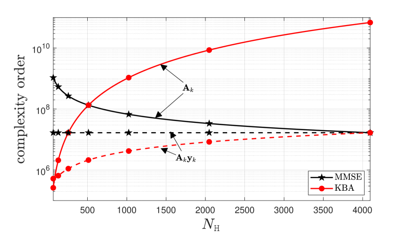
Figure 9: Complexity order as a function of the UPA shape (fixed size $N=4096$).

VII-D Summary

The above results are summarized in Table III, which also contains the complexity for the DFT-based method derived in Sect. V (please refer to [1] for more details on the complexity associated to this technique). Each column contains the complexity associated to each of the three phases in the channel estimation process. In particular, we focus on the computation of $\boldsymbol{\mathbf{A}}_{k}$ and $\boldsymbol{\mathbf{A}}_{k}\boldsymbol{\mathbf{y}}_{k}$, which are the two phases in which the MMSE and the KBA differ. To better illustrate the impact of the UPA size on the computational burden, Figure 9 reports the complexity as a function of $N_{\mathsf{H}}$ in an UPA with size $N=4096$. We see that the complexity for the computation of $\boldsymbol{\mathbf{A}}_{k}\boldsymbol{\mathbf{y}}_{k}$ is always lower with KBA, regardless of the shape of the array. Different conclusions hold for the computation of $\boldsymbol{\mathbf{A}}_{k}$. In particular, for nearly square UPA configurations (especially when $N^{0.25}\leq N_{\mathsf{H}}\leq N^{0.75}$ – e.g., $8\leq N_{\mathsf{H}}\leq 512$ when $N=4096$), the KBA-based approach (red line) provides less complexity than the MMSE one (black line), while the situation is reversed for near ULA configurations: In particular, when $N_{\mathsf{V}}$ is equal to $1$, the gap is at its maximum; in this case, however, we can resort to the DFT-based approach, which gives a significant complexity saving (more than three orders of magnitude with $N=4096$). Interestingly, when $N_{\mathsf{H}}=\sqrt{N}$, the complexity saving provided by KBA is maximal and equal to $N$, thus supporting scalability for square UPAs with a very large number of antennas. Moreover, since the update interval of $\boldsymbol{\mathbf{A}}_{k}$ is of the same order of magnitude as the channel coherence time, this strengthens the conclusions drawn in Sect. VI-B regarding the suitability of the proposed method in highly time-varying scenarios. Conversely, there are (few) situations where the KBA-based approach requires a larger number of operations: in the example above, when $N=4096$, this situation occurs for $N_{\mathsf{H}}=1024$ and $N_{\mathsf{H}}=2048$.

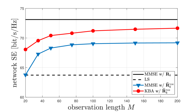
(a) RZF combining.

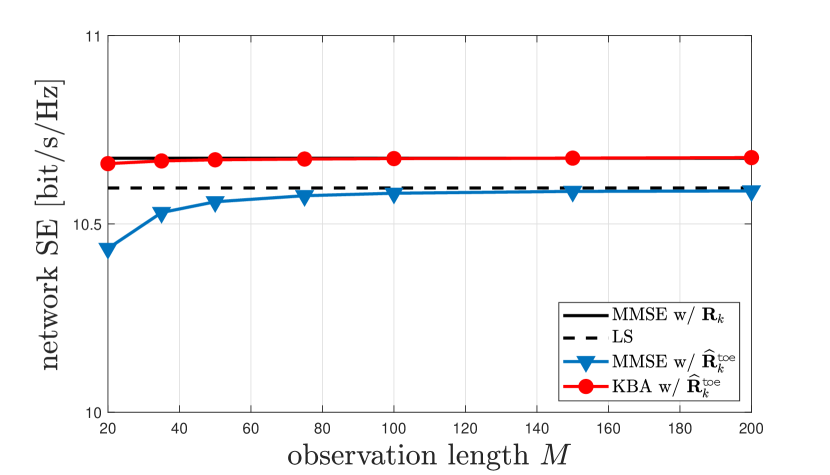
(b) MR combining.

Figure 10: Sum-SE as a function of the observation length $M$ with MR and RZF combining.

Sect. VIII Uplink spectral efficiency evaluation

Channel estimation is the ancillary task to support data detection, which is the ultimate goal of a communication system. Hence, we now compare the investigated solutions in terms of achievable uplink SE. This is obtained with the well-known use-and-then-forget bound [2, Sect. 4.2], which yields

$$\underline{\mathsf{SE}}_{k}=\left(1-\frac{\tau_{p}}{\tau_{c}}\right)\mathbb{E}\left\{{\log_{2}\left(1+\underline{\gamma}_{k}\right)}\right\}\qquad\textrm{[bit/s/Hz]},$$ (54)

where the factor ${\tau_{p}}/{\tau_{c}}$ accounts for the fraction of samples per coherence block used for channel estimation, with $\tau_{c}$ being the length of each coherence block, and $\underline{\gamma}_{k}$ is given by

$$\frac{\left|\mathbb{E}\left\{{\boldsymbol{\mathbf{v}}_{k}^{\mathsf{H}}\boldsymbol{\mathbf{h}}_{k}}\right\}\right|^{2}}{\sum_{i=1}^{K}{\mathbb{E}\left\{{\left|\boldsymbol{\mathbf{v}}_{k}^{\mathsf{H}}\boldsymbol{\mathbf{h}}_{i}\right|^{2}}\right\}}-\left|\mathbb{E}\left\{{\boldsymbol{\mathbf{v}}_{k}^{\mathsf{H}}\boldsymbol{\mathbf{h}}_{k}}\right\}\right|^{2}+\frac{\sigma^{2}}{\rho}\mathbb{E}\left\{{\left\|\boldsymbol{\mathbf{v}}_{k}\right\|^{2}}\right\}},$$ (55)

with $\boldsymbol{\mathbf{v}}_{k}\in\mathbb{C}^{N}$ being the receive combining vector associated to UE $k$. Notice that the expectations are computed with respect to all sources of randomness. We consider both regularized zero forcing (RZF) combining, according to which

$$\boldsymbol{\mathbf{v}}_{k}=\left(\sum_{i=1}^{K}{\widehat{\boldsymbol{\mathbf{h}}}_{i}\widehat{\boldsymbol{\mathbf{h}}}_{i}^{\mathsf{H}}}+\frac{\sigma^{2}}{\rho}\boldsymbol{\mathbf{I}}_{N}\right)^{-1}\widehat{\boldsymbol{\mathbf{h}}}_{k}$$ (56)

and maximum ratio (MR) combining $\boldsymbol{\mathbf{v}}_{k}=\widehat{\boldsymbol{\mathbf{h}}}_{k}$.

Figure 10 shows the network SE, given by

$$\underline{\mathsf{SE}}=\sum_{k=1}^{K}\underline{\mathsf{SE}}_{k}\qquad\textrm{[bit/s/Hz].}$$ (57)

as a function of the observations $M$ used to estimate the channel statistics. The RZF combining scheme (56) is used in Figure 10(a), while MR is adopted in Figure 10(b). The network parameters are detailed in Tables I and II, with $K=10$ randomly placed UEs. The black solid line corresponds to the MMSE estimator using perfect knowledge of the channel statistics $\boldsymbol{\mathbf{R}}_{k}$ for both the combining and the estimation schemes (i.e., the estimation makes use of true $\boldsymbol{\mathbf{R}}_{k}$), whereas the black dashed line depicts the results using the LS estimator (11); blue and red lines correspond to the results obtained assuming imperfect channel statistics for the MMSE and the KBA methods, respectively, and thus $\boldsymbol{\mathbf{R}}_{k}$ (used for both estimation and combining) is estimated using the methods introduced in Sect. VI: more in detail, the MMSE estimator uses (38) with $\eta=0.8$, whereas the KBA-based estimator uses (48) (without any regularization parameter $\eta$).

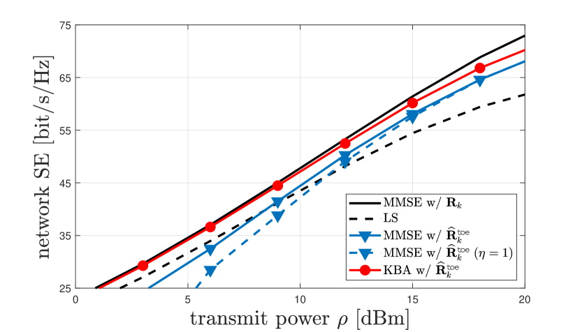
Figure 11: Sum-SE with RZF as a function of the transmit power $\rho$.

We notice that, while the gap between the imperfect-knowledge MMSE estimator (blue line) and the benchmark curves remains significant even for large values of $M$, the performance of the KBA-based scheme (red line) is very close to the optimal one (black curve), even for moderately low values of $M$ (for MR combining, there is no difference, whereas the MMSE shows some gap, yet much smaller than that provided by the MMSE estimator with imperfect knowledge, and decreasing with $M$). This confirms the results presented in Sect. VI-B, in which the KBA-based method, thanks to a simpler structure, introduces more robustness compared to the MMSE counterpart for the same observation length $M$, and makes it more suitable for more dynamic scenarios, in which the coherence time is reduced (and hence $M$ needs to be kept as low as possible). In addition, the KBA-based method does not call for any numerical optimization of the regularization parameter $\eta$ (unlike the MMSE estimator – see comments to Figure 7), and it can thus be universally adopted, irrespectively of the network setup (including UPA parameters).

Figure 11 shows the network SE with RZF as a function of the transmit power $\rho$. The network setup is identical to the one considered for Figure 10(a), assuming $M=50$ channel observations for the covariance matrix estimation task. As can be seen, when $\rho=20\,\mathrm{dBm}$ (i.e., the same parameter setup considered for Figure 10(a)), the KBA-based method outperforms the MMSE one by $1.7\,\textrm{bit/s/Hz}$. Only when increasing $\rho$, in particular when $\rho\geq 26\,\mathrm{dBm}$ (not reported here in the figure), in this simulation setup the two methods provide approximately the same performance. This means that the proposed KBA method is particularly suitable in low-SNR regimes, in which the link budget does not guarantee sufficient accuracy for the MMSE counterpart. Similar trends, not reported here for the sake of brevity, are observed for MR combining.

Sect. IX Conclusion

We developed channel estimation schemes for large-scale MIMO systems that achieve accuracy levels comparable to the optimal MMSE estimator, while also offering reduced complexity and enhanced robustness to the imperfect knowledge of channel statistics. Both UPAs and ULAs were studied. In the case of UPAs, we exploited the inherent structure of the spatial correlation matrix to approximate it by a Kronecker product, and in the case of ULAs, we used a circulant approximation to further reduce the computational complexity. Comparisons were made with the optimal MMSE estimator and other alternatives with less complexity (e.g., the LS estimator). Numerical results confirmed the effectiveness of the proposed methods in terms of UL SE with various combining schemes, approaching MMSE performance while significantly reducing computational complexity. Specifically, the computational load scales as $N\sqrt{N}$ and $N\log N$ for squared planar arrays and linear arrays, respectively. Furthermore, the proposed schemes exhibited improved robustness in scenarios with imperfect channel statistics and low-to-medium SNR scenarios.

Appendix

The estimation of $\boldsymbol{\mathbf{h}}_{k}$ calls for the product between $\boldsymbol{\mathbf{A}}_{k}$ and $\boldsymbol{\mathbf{y}}_{k}$. Accordingly, when $\boldsymbol{\mathbf{A}}_{k}$ is written as a product of matrices (as occurs, for instance, with the MMSE or the KBA estimators), it is convenient not to perform the products. Indeed, assume that we have to compute $\boldsymbol{\mathbf{B}}_{1}\boldsymbol{\mathbf{B}}_{2}\boldsymbol{\mathbf{b}}$, where $\boldsymbol{\mathbf{B}}_{1}$ and $\boldsymbol{\mathbf{B}}_{2}$ are $N\times N$ matrices and $\boldsymbol{\mathbf{b}}$ is an $N$-dimensional vector. If we first multiply $\boldsymbol{\mathbf{B}}_{1}$ and $\boldsymbol{\mathbf{B}}_{2}$, and then the resulting matrix and $\boldsymbol{\mathbf{b}}$, we have to perform $N^{3}+N^{2}$ multiplications and $(N-1)N^{2}+(N-1)N$ additions. On the other hand, if we first compute the product between $\boldsymbol{\mathbf{B}}_{2}$ and $\boldsymbol{\mathbf{b}}$, and then the product between $\boldsymbol{\mathbf{B}}_{1}$ and the resulting vector, $2N^{2}$ multiplications and $2(N-1)N$ additions are needed. This means, for example, that when considering the MMSE estimator it is better to compute first $(\widehat{\boldsymbol{\mathbf{Q}}}_{k}^{\mathsf{toe}})^{-1}\boldsymbol{\mathbf{y}}_{k}$ and then $\widehat{\boldsymbol{\mathbf{R}}}^{\mathsf{toe}}_{k}\left[(\widehat{\boldsymbol{\mathbf{Q}}}_{k}^{\mathsf{toe}})^{-1}\boldsymbol{\mathbf{y}}_{k}\right]$. An analogous approach can be conveniently used with the KBA estimator. Another useful result, that can be exploited to reduce the complexity of the KBA estimator, concerns the computation of the product $(\boldsymbol{\mathbf{C}}_{1}\otimes\boldsymbol{\mathbf{C}}_{2})\boldsymbol{\mathbf{b}}$, where $\boldsymbol{\mathbf{C}}_{1}$ is $m\times m$, $\boldsymbol{\mathbf{C}}_{2}$ is $n\times n$, and $\boldsymbol{\mathbf{b}}$ is an $mn$-dimensional vector. The evaluation of $(\boldsymbol{\mathbf{C}}_{1}\otimes\boldsymbol{\mathbf{C}}_{2})\boldsymbol{\mathbf{b}}$ can efficiently be performed with $(m+n)mn$ floating-point operations instead of $m^{2}n^{2}$ [30].

References

- [1] A. A. D’Amico, G. Bacci, and L. Sanguinetti, “DFT-based channel estimation for holographic MIMO,” in Proc. Asilomar Conf. Signals, Systems, and Computers, Pacific Grove, CA, Oct.-Nov. 2023.
- [2] E. Björnson, J. Hoydis, and L. Sanguinetti, “Massive MIMO networks: Spectral, energy, and hardware efficiency,” Foundations and Trends® in Signal Processing, vol. 11, no. 3-4, pp. 154–655, 2017.
- [3] E. Björnson, L. Sanguinetti, H. Wymeersch, J. Hoydis, and T. L. Marzetta, “Massive MIMO is a reality – What is next?” Digit. Signal Process., vol. 94, no. C, pp. 3–20, nov 2019. [Online]. Available: https://doi.org/10.1016/j.dsp.2019.06.007
- [4] L. Sanguinetti, E. Björnson, and J. Hoydis, “Toward massive MIMO 2.0: Understanding spatial correlation, interference suppression, and pilot contamination,” IEEE Trans. Commun., vol. 68, no. 1, pp. 232–257, 2020.
- [5] Z. Wang, J. Zhang, H. Du, W. E. I. Sha, B. Ai, D. Niyato, and M. Debbah, “Extremely large-scale MIMO: Fundamentals, challenges, solutions, and future directions,” IEEE Wireless Communications, pp. 1–9, 2023.
- [6] E. Björnson, C.-B. Chae, R. W. Heath, T. L. Marzetta, A. Mezghani, L. Sanguinetti, F. Rusek, M. R. Castellanos, D. Jun, and O. T. Demir, “Towards 6G MIMO: Massive spatial multiplexing, dense arrays, and interplay between electromagnetics and processing,” 2024.
- [7] J. An, C. Yuen, C. Huang, M. Debbah, H. V. Poor, and L. Hanzo, “A tutorial on holographic MIMO communications – part I: Channel modeling and channel estimation,” IEEE Commun. Letters, vol. 27, no. 7, pp. 1664–1668, 2023.
- [8] J. An, C. Xu, L. Gan, and L. Hanzo, “Low-complexity channel estimation and passive beamforming for RIS-assisted MIMO systems relying on discrete phase shifts,” IEEE Trans. Commun., vol. 70, no. 2, pp. 1245–1260, 2022.
- [9] Y. Liu, Z. Tan, H. Hu, L. J. Cimini, and G. Y. Li, “Channel estimation for OFDM,” IEEE Commun. Surv. Tut., vol. 16, no. 4, pp. 1891–1908, 2014.
- [10] F. Dai and J. Wu, “Efficient broadcasting in ad hoc wireless networks using directional antennas,” IEEE Trans. Parallel Distrib. Syst., vol. 17, no. 4, pp. 335–347, 2006.
- [11] Z. Xiao, T. He, P. Xia, and X.-G. Xia, “Hierarchical codebook design for beamforming training in millimeter-wave communication,” IEEE Trans. Wireless Commun., vol. 15, no. 5, pp. 3380–3392, 2016.
- [12] J. Zhang, Y. Huang, Q. Shi, J. Wang, and L. Yang, “Codebook design for beam alignment in millimeter wave communication systems,” IEEE Trans. Commun., vol. 65, no. 11, pp. 4980–4995, 2017.
- [13] S. Noh, M. D. Zoltowski, and D. J. Love, “Multi-resolution codebook and adaptive beamforming sequence design for millimeter wave beam alignment,” IEEE Trans. Wireless Commun., vol. 16, no. 9, pp. 5689–5701, 2017.
- [14] Z. Wan, Z. Gao, F. Gao, M. Di Renzo, and M.-S. Alouini, “Terahertz massive MIMO with holographic reconfigurable intelligent surfaces,” IEEE Trans. Commun., vol. 69, no. 7, pp. 4732–4759, 2021.
- [15] M. Cui and L. Dai, “Channel estimation for extremely large-scale MIMO: Far-field or near-field?” IEEE Trans. Commun., vol. 70, no. 4, pp. 2663–2677, 2022.
- [16] M. Ghermezcheshmeh and N. Zlatanov, “Parametric channel estimation for LoS dominated holographic massive MIMO systems,” IEEE Access, pp. 44 711–44 724, 2023.
- [17] Ö. T. Demir, E. Björnson, and L. Sanguinetti, “Channel modeling and channel estimation for holographic massive MIMO with planar arrays,” IEEE Wireless Commun. Lett., vol. 11, no. 5, pp. 997–1001, 2022.
- [18] A. Pizzo, L. Sanguinetti, and T. L. Marzetta, “Fourier plane-wave series expansion for holographic MIMO communications,” IEEE Trans. Wireless Commun., vol. 21, no. 9, pp. 6890–6905, 2022.
- [19] E. Björnson, L. Sanguinetti, and M. Debbah, “Massive MIMO with imperfect channel covariance information,” in Proc. Asilomar Conf. Signals, Systems and Computers, Pacific Grove, CA, USA, 2016, pp. 974–978.
- [20] C. Van Loan and N. Pitsianis, “Approximation with Kronecker products,” in Linear Algebra for Large Scale and Real Time Applications, M. S. Moonen and G. H. Golub, Eds. Dordrecht, The Netherlands: Kluwer Publications, 1992, pp. 293–314.
- [21] C. F. Van Loan, “The ubiquitous Kronecker product,” J. Computational and Applied Mathematics, vol. 123, pp. 85–100, 2000.
- [22] J. Pearl, “Basis-restricted transformations and performance measures for spectral representations (corresp.),” IEEE Trans. Information Theory, vol. 17, no. 6, pp. 751–752, 1971.
- [23] ——, “On coding and filtering stationary signals by discrete fourier transforms (corresp.),” IEEE Trans. Information Theory, vol. 19, no. 2, pp. 229–232, 1973.
- [24] Z. Zhu and M. B. Wakin, “On the asymptotic equivalence of circulant and Toeplitz matrices,” IEEE Trans. Information Theory, vol. 63, no. 5, pp. 2975–2992, 2017.
- [25] E. Björnson and L. Sanguinetti, “Rayleigh fading modeling and channel hardening for reconfigurable intelligent surfaces,” IEEE Wireless Commun. Letters, vol. 10, no. 4, pp. 830–834, 2021.
- [26] A. Sayeed, “Deconstructing multiantenna fading channels,” IEEE Trans. Signal Process., vol. 50, no. 10, pp. 2563–2579, 2002.
- [27] R. Zhang, X. Lu, J. Zhao, L. Cai, and J. Wang, “Measurement and modeling of angular spreads of three-dimensional urban street radio channels,” IEEE Trans. Veh. Technol., pp. 3555–3570, 2017.
- [28] M. Wax and T. Kailath, “Efficient inversion of Toeplitz-block Toeplitz matrix,” IEEE Trans. Acoustics, Speech, and Signal Process., vol. 31, no. 5, pp. 1218–1221, 1983.
- [29] F. W. Trench, “Numerical solution of the eigenvalue problem for Hermitian Toeplitz matrices,” SIAM J. Matrix Analysis and Applications, vol. 10, no. 2, pp. 135–146, 1989.
- [30] T. Dayar and M. C. Orhan, “On vector-kronecker product multiplication with rectangular factors,” SIAM J. Scientific Computing, vol. 37, no. 5, pp. S526–S543, 2015. [Online]. Available: https://doi.org/10.1137/140980326