Matrix-Free Geometric Multigrid Preconditioning Of Combined Newton-GMRES For Solving Phase-Field Fracture With Local Mesh Refinement

Abstract

In this work, the matrix-free solution of quasi-static phase-field fracture problems is further investigated. More specifically, we consider a quasi-monolithic formulation in which the irreversibility constraint is imposed with a primal-dual active set method. The resulting nonlinear problem is solved with a line-search assisted Newton method. Therein, the arising linear equation systems are solved with a generalized minimal residual method (GMRES), which is preconditioned with a matrix-free geometric multigrid method including geometric local mesh refinement. Our solver is substantiated with a numerical test on locally refined meshes.

1 Introduction

This work is devoted to the efficient linear solution within the nonlinear solver of quasi-static phase-field fracture problems. Phase-field fracture remains a timely topic with numerous applications. Therein, vector-valued displacements and a scalar-valued phase-field variable couple. Moreover, the phase-field variable is subject to a crack irreversibility constraint. Due to nonlinear couplings, nonlinear constitutive laws and the previously mentioned irreversibility constraint, the overall coupled problem is nonlinear. Here, a line-search assisted Newton method is employed. Therein, the linear solution often is a point of concern.

Based on prior work [14], a GMRES (generalized minimal residual method) iterative linear solver is employed. This is preconditioned with a matrix-free geometric multigrid (GMG) method. In the matrix-free context, the system matrix is not fully assembled [19] and reduces the memory consumption. At the same time, this limits the choice of available smoothers for the multigrid preconditioner. Here, a Chebyshev-Jacobi smoother is employed as it only requires matrix-vector products and an estimate of the largest eigenvalue. Moreover, the inverse diagonal of the system matrix is required, which however can be obtained from the local assembly without required the entire matrix. With these ingredients a matrix-free solution can be set up. Recent works of matrix-free solvers include problems in finite-strain hyperelasticity [7], phase-field fracture [15, 14], Stokes [16], generalized Stokes [29], fluid-structure interaction [30], discontinuous Galerkin [20], compressible Navier-Stokes equations [10], incompressible Navier-Stokes and Stokes equations [9] as well as sustainable open-source code developments [24, 6], matrix-free implementations on locally refined meshes [23], implementations on graphics processors [21], and performance-portable methods on CPUs and GPUs applied to solid mechanics [5]. The main contribution of this work is that we combine a GMG preconditioner with locally refined meshes and primal-dual active set for the inequality constraint of phase-field fracture using local smoothing [13]. Our overall numerical solver is applied to one numerical test, namely Sneddon’s example that is nowadays considered as a benchmark [26]. The outline of these conference proceedings is as follows. In Section 2 the phase-field problem is stated. Then, in Section 3, the numerical solutions are explained, namely the nonlinear solution via a combined Newton method and the linear solution with GMRES and matrix-free geometric multigrid preconditioning. Finally, in Section 4 a numerical test substantiates our developements.

2 Problem Formulation: The Phase-Field Model

This section introduces the problem formulation for phase-field fracture which was originally formulated as an energy minimization problem [8]. However, our starting point are the variational Euler-Lagrange equations. For this, we provide basic notations: given a sufficiently smooth material $\Omega\subset\mathbb{R}^{d}$, $d=2$, the scalar-valued and vector-valued $L^{2}$-products over a smooth bounded domain $G\subset\Omega$ are defined by

$$(x,y)_{L^{2}(G)}\coloneqq\int_{G}x\cdot ydG,\quad(X,Y)_{L^{2}(G)}\coloneqq\int_{G}X:YdG,$$ (1)

where $X:Y$ denote the Frobenius product of two vector fields. If there is no subscript provided, $L^{2}$-product over the whole material domain $\Omega$ is meant. Energy minimization problems in the phase-field fracture context (e.g. [4, 22]) usually consist of a displacement variable $u:\Omega\rightarrow\mathbb{R}^{d}$ and a phase-field variable $\varphi:\Omega\rightarrow[0,1]$. The phase-field variable $\varphi$ can be understood as an indicator function: It is defined such that $\varphi=0$ where the material is fully broken and $\varphi=1$ where it is intact. Only allowing a fully broken or a completely intact domain leads to discontinuities, which is treated by the Ambrosio-Tortorelli approximation [1, 2]. With this, we introduce a transition zone where $0<\varphi<1$ of width $2l$. In the following $l$ is called the length-scale parameter. Deriving the Euler-Langrange equations from computing directional derivatives, the solution sets on the continuous level are given by $\mathcal{V}\coloneqq H^{1}_{0}(\Omega),\mathcal{K}^{n}\coloneqq\{\psi\in\mathcal{W}\,|\,\psi-\varphi^{n-1}\leq 0\text{ a.e. in }\Omega\}$, where $\mathcal{W}\coloneqq H^{1}(\Omega)$. The function space $\mathcal{K}^{n}$ is a convex set arising from the crack irreversibility constraint $\partial_{t}\varphi\leq 0$. In the quasi-static setting, this translates to $\varphi^{n}\leq\varphi^{n-1}$ with $\varphi^{n}:=\varphi(t_{n})$ and $\varphi^{n-1}:=\varphi(t_{n-1})$. This results in an incremental grid $t_{0},\dots t_{N}$ with the step-size $k_{n}=t_{n}-t_{n-1}$, where $t_{0}$ is the initial configuration and $t_{N}$ the end-time configuration. The Euler-Lagrange equations are then given by [22, 31, 18]:

Problem 1.

For some given initial value $\varphi^{0}$ and for the incremental steps $t_{n}$ with $n=1,...,N$, find $(u^{n},\varphi^{n})\in\mathcal{V}\times\mathcal{K}^{n}$ such that for all $\psi^{u}\in\mathcal{V}$ and $\psi^{\varphi}\in\mathcal{K}^{n}\cap L^{\infty}(\Omega)$

$$\begin{split}\left(g(\varphi^{n})\sigma(u^{n}),e(\psi^{u})\right)+((\varphi^{n})^{2}p^{n},\operatorname{div}\psi^{u})&=0,\end{split}$$ (2)

$$\begin{split}(1-\kappa)(\varphi^{n}\sigma(u^{n}):e(u^{n}),\psi^{\varphi}-\varphi^{n})+2(\varphi^{n}p^{n}\operatorname{div}u^{n},\psi^{\varphi}-\varphi^{n})&\quad\\ \qquad+G_{C}\left(\frac{1}{l}(1-\varphi^{n},\psi^{\varphi}-\varphi^{n})+l(\nabla\varphi^{n},\nabla(\psi^{\varphi}-\varphi^{n}))\right)&\geq 0,\end{split}$$ (3)

where $p\in L^{\infty}(\Omega)$ is a given pressure, $G_{C}>0$ is the critical energy release rate and $\kappa>0$ is a regularization parameter. A study on how to find a proper setting for $\kappa$ and the length-scale parameter $l$ is given in [17]. The classical stress tensor of linearized elasticity $\sigma(u)$ and the symmetric strain tensor $e(u)$ are given by

$$\sigma(u)\coloneqq 2\mu e(u)+\lambda\operatorname{tr}(e(u))I,\quad e(u)\coloneqq\frac{1}{2}\left(\nabla u+\nabla u^{T}\right),$$ (4)

with the Lamé parameters $\mu>0$ and $\lambda$ with $3\lambda+2\mu>0$ and the identity Matrix $I$. Lastly, the degradation function $g(\varphi^{n})$ is defined by $g(\varphi^{n}):=(1-\kappa)(\varphi^{n})^{2}+\kappa$.

To enhance the robustness of the nonlinear solution, we linearize the degradation function following [11, 18]. Therein, the phase-field $\varphi^{n}$ is replaced by the old incremental step solution or an extrapolation using previous incremental step solutions. Equation (2) reads then

$$\left(g(\tilde{\varphi}^{n})\sigma(u^{n}),e(\psi^{u})\right)+((\tilde{\varphi}^{n})^{2}p^{n},\operatorname{div}\psi^{u})=0.$$ (5)

The second difficulty of the above problem is the fact that we have to deal with a constraint variational inequality system (CVIS). This inequality system can be equivalently formulated as an equality constraint system with an additional complementarity equation [18]:

Problem 2.

For a given initial condition $\varphi^{0}$ and for the incremental steps $t_{n}$ with $n=1,...,N$, find $U^{n}=\{u^{n},\varphi^{n}\}\in\mathcal{V}\times\mathcal{W}$ and $\lambda^{n}\in\mathcal{N}_{+}$ such that

$$A(U^{n})(\Psi)+(\lambda^{n},\psi^{\varphi}) =0\quad\forall\Psi=\{\psi^{u},\psi^{\varphi}\}\in\mathcal{V}\times\mathcal{W}\cap L^{\infty},$$

$$C(\varphi^{n},\lambda^{n}) =0\quad\text{a.e.\ in }\Omega,$$

with

$$\begin{split}A(U^{n})(\Psi)&\coloneqq\left(g(\tilde{\varphi}^{n})\sigma^{+}(u^{n}),e(\psi^{u})\right)+((\tilde{\varphi}^{n})^{2}p^{n},\operatorname{div}\psi^{u})\\ &\quad+(1-\kappa)(\varphi^{n}\sigma^{+}(u^{n}):e(u^{n}),\psi^{\varphi}-\varphi^{n})+2(\varphi^{n}p^{n}\operatorname{div}u^{n},\psi^{\varphi})\\ &\quad+G_{C}\left(\frac{1}{l}(1-\varphi^{n},\psi^{\varphi}-\varphi^{n})+l(\nabla\varphi^{n},\nabla(\psi^{\varphi}))\right),\end{split}$$ (6)

and

$$C(\varphi^{n},\lambda^{n})\coloneqq\lambda^{n}-\max\{0,\,\lambda^{n}+c(\varphi^{n}-\varphi^{n-1})\}.$$ (7)

The solution set $\mathcal{N}_{+}$ for the Lagrange multiplier is defined by

$$\mathcal{N}_{+}\coloneqq\left\{\mu\in L^{2}(\Omega)\,|\,(\mu,v)_{L^{2}(\Omega)}\leq 0\quad\forall v\in L^{2}_{-}(\Omega)\right\}.$$ (8)

This formulation is the starting point for a primal-dual active set (PDAS) method, which we use to treat the irreversibility condition. The idea is to split the domain, based on the structure of the complementarity condition, into two subdomains: The active set $\mathcal{A}$, where the constraint is active, i.e. the phase-field variable does not change, and the inactive set $\mathcal{I}$, where the constraint is inactive. In the latter, the problem can be treated and solved as an unconstrained problem. The active and inactive sets at each incremental step are defined such as

$$\lambda^{n}+c(\varphi^{n}-\varphi^{n-1}) \leq 0\text{ a.e.\ in }\mathcal{I}^{n},$$ (9)

$$\lambda^{n}+c(\varphi^{n}-\varphi^{n-1}) >0\text{ a.e.\ in }\mathcal{A}^{n}.$$ (10)

The active set constant $c$ can be chosen arbitrarily. However, in other contributions [12, 25, 27], the authors state that it can have an influence on the performance. Following our prior work [18], we set $c$ as

$$c=c^{k}\coloneqq 2\left|\frac{\lambda_{h,i}^{k}}{(\varphi_{h,i}^{k}-\varphi_{h,i}^{\operatorname{old}})}\right|.$$ (11)

3 Nonlinear Solution With Inner Linear GMRES Iterative Solver And Matrix-Free Geometric Multigrid Preconditioning

This section describes the numerical methods we use to solve the introduced variational phase-field fracture problem. As discretization, we employ a finite element method with $H^{1}$-conforming bilinear finite elements for both the displacement and the phase-field, as an outer solver, we employ a combined Newton active set method and as an inner linear solver, we utilize a GMRES algorithm together with a geometric multigrid preconditioner. The newly developed code is implemented in a matrix-free framework using the finite element library deal.II [3]. Related work having deal.II as well as basis was done in [14, 15].

3.1 A Combined Newton Type Algorithm

In each incremental step, the Newton iteration to solve for $U^{n}\coloneqq\{u^{n},\varphi^{n}\}\in\mathcal{V}\times\mathcal{W}$ and $\lambda^{n}\in\mathcal{N}_{+}$ is given by

$$A^{\prime}(U^{n,k})(\delta U^{n,k+1},\Psi)+(\lambda^{n,k},\psi^{\varphi})=-A(U^{n,k})(\Psi)\quad\forall\Psi\in\mathcal{V}\times\mathcal{W},$$

which is solved with respect to

$$C(\varphi^{n,k}+\delta\varphi^{n,k+1},\lambda^{n,k})=0\quad\text{ a.e.\ in }\Omega,$$

for the Newton update $\delta U^{n,k+1}$ and the Lagrange multiplier $\lambda^{n,k+1}$. The solution is then updated via

$$U^{n,k+1}=U^{n,k}+\delta U^{n,k+1}.$$

The Jacobian $A^{\prime}(U^{n,k})(\delta U^{n,k+1},\Phi)$ is given by

$$\begin{split}A^{\prime}(U^{n,k})&(\delta U^{n,k+1},\Psi)=\left(g(\tilde{\varphi}^{n})\sigma(\delta u^{n,k+1}),e(\psi^{u})\right)\\ &+(1-\kappa)\left(\delta\varphi^{n,k+1}\sigma(u^{n,k}):e(u^{n,k})+2\varphi^{n,k}\sigma(\delta u^{n,k+1}):e(u^{n,k}),\psi^{\varphi}\right)\\ &+2p\left(\delta\varphi^{n,k+1}\operatorname{div}u^{n,k}+\varphi^{n,k}\operatorname{div}\delta u^{n,k+1},\psi^{\varphi}\right)\\ &+G_{C}\left(\frac{1}{l}(\delta\varphi^{n,k+1},\psi^{\varphi})+l(\nabla\delta\varphi^{n,k+1},\nabla\psi^{\varphi})\right).\end{split}$$

In combination with an iteration on the active set, we obtain scheme outlined in Algorithm 1.

Algorithm 1 (Primal-dual active set method)

1:Set iteration index $k=0$

2:while $\mathcal{A}^{n,k}\neq\mathcal{A}^{n,k+1}$ do

3:     Determine the active set $\mathcal{A}^{n,k}$ and inactive set $\mathcal{I}^{n,k}$ with (9), (10)

4:     Find $\delta U^{n,k+1}\in\mathcal{V}\times\mathcal{W}$ and $\lambda^{n,k+1}\in\mathcal{N}_{+}$ with solving

$$A^{\prime}(U^{n,k})(\delta U^{n,k+1},\Phi)+(\lambda^{n,k+1},\psi) =-A(U^{n,k})(\Phi),\quad\forall\Phi\coloneqq\{v,\psi\}\in\mathcal{V}\times\mathcal{W},$$

$$\delta\varphi^{n,k+1} =0\quad\text{ on }\mathcal{A}^{k},$$

$$\lambda^{n,k+1} =0\quad\text{ on }\mathcal{I}^{k}.$$

5:     Update the solution to obtain $U^{n,k+1}$ via

$$U^{n,k+1}=U^{n,k}+\delta U^{n,k+1}.$$

6:     Update iteration index $k=k+1$

The combined Newton active Fracture With set algorithm has two stopping criteria which have to be fulfilled: On one hand, the Newton residual has to be small enough while on the other hand the active set has to remain unchanged over two consecutive iterations. With the active set convergence, we ensure that we indeed applied the constraints in the right way.

3.2 A Geometric Multigrid Block Preconditioner For GMRES

In a matrix-free framework, only iterative methods which solely rely on matrix-vector products are applicable as smoothers. We choose a Chebyshev-accelerated polynomial Jacobi smoother. This method requires to precompute the inverse diagonal entries of the system matrix (i.e. the Jacobian) and an estimate for the eigenvalues. The latter can be obtained by employing a conjugate gradient method. On the finer grid, we are mainly interested in smoothing out the highly oscillating error parts, thus it suffices to compute the maximal eigenvalue and then approximate the smoothing range by $[\lambda_{\min},\lambda_{\max}]\approx[\rho\lambda_{\min},1.2\lambda_{\max}]$ with $\rho<1$. On the coarse grid, we then compute both the maximal and the minimal eigenvalue for indeed solving the problem. We apply the preconditioner on the whole block system by performing 1 V-cycle on each of the symmetric positive definite diagonal blocks as follows. On locally refined meshes, we employ local smoothing, where the smoothing on each level is restricted to the interior of the level domains. We want to solve the following preconditioned inner linear system arising from finite element discretization and Newton’s method

$$P^{-1}\tilde{G}\delta U=P^{-1}\tilde{R},$$ (12)

with

$$G\coloneqq\begin{bmatrix}\tilde{G}^{uu}&0\\ \tilde{G}^{u\varphi}&\tilde{G}^{\varphi\varphi}\end{bmatrix}.$$ (13)

The preconditioner $P^{-1}$ is then constructed as

$$P^{-1}\coloneqq\begin{bmatrix}MG(\tilde{G}^{uu})&0\\ 0&MG(\tilde{G}^{\varphi\varphi})\end{bmatrix},$$ (14)

with the mentioned Jacobi-Block smoother applied to each diagonal block. One challenge of the multigrid preconditioner is to transfer the information of possible constraints onto the coarser grids. In our case, we have to deal with 3 different types of constraints: Boundary conditions, active set constraints and hanging node constraints. The latter arise may arise in the case of the adaptive mesh refinement. The constraints can be transferred to coarser grid in a canonical way. For instance, for the active set, those degrees of freedom which are constrained on finer grids are also constrained on coarser grids.

3.3 The Matrix-Free Approach And Final Algorithm

The full Algorithm 2 is realized in a matrix-free framework to reduce the memory consumption. From the implementation point of view, the concept is simple: Instead of assembling and storing the system matrix, we implement a linear operator which represents the application of the matrix to a vector. For this, the global matrix-vector-product can be split into local matrix-vector-products corresponding to the underlying finite elements. As previously mentioned, the implementation is realized with deal.II, which offers a toolbox of functionalities considering matrix-free finite-element approaches [19].

Algorithm 2 full algorithm

1:Setup the system $\triangleright$ initialize grid $\mathcal{T}_{h}$, parameters, etc.

2:for $n=1,2,...$ do$\triangleright$ timestep loop

3:     while $\left(\mathcal{A}^{n,k-1}\neq\mathcal{A}^{n,k}\right)$ or $\left(\tilde{R}(U_{h}^{n,k})>\text{TOL}_{N}\right)$ do

4:         Compute the active set $\mathcal{A}^{n,k}=\left\{x_{i}\bigg{|}\left[B\right]_{ii}^{-1}\left[R(U_{h}^{n,k})\right]_{i}+c(\varphi_{h,i}^{n,k}-\varphi_{h,i}^{n-1})>0\right\}$

5:         Set the active set constraints for the Newton update: $\delta\varphi_{i}^{n,k+1}=\varphi_{i}^{n-1}-\varphi_{i}^{n,k}$

6:         Set constraints for Newton update and assemble the residual $R(U_{h}^{n,k})$

7:         Setup the Multigrid preconditioner

8:         Solve the inner linear system with GMRES and GMG preconditioner

9:         Distribute the constraints on the Newton update

10:         Choose maximum number of line search iterations $l_{\max}$

11:         Choose line search damping parameter $0<\omega\leq 1$

12:         for $l=1:l_{\max}$ do

13:              Update the solution with $U_{h}^{n,k+1}=U_{h}^{n,k}+\delta U_{h}^{n,k+1}$

14:              Assemble the new residual $\tilde{R}(U_{h}^{n,k+1})$

15:              if $\lVert\tilde{R}(U_{h}^{n,k+1})\rVert_{2}<\lVert\tilde{R}(U_{h}^{n,k})\rVert_{2}$ then

16:                  break

17:              else

18:                  Adjust the Newton update with $\delta U_{h}^{n,k+1}:=\omega^{l}\delta U_{h}^{n,k+1}$                        

19:         Update iteration index $k=k+1$      

4 Numerical Test: Sneddon’s Benchmark

In this section, we present numerical results for a stationary two dimensional benchmark test, where a one dimensional crack is prescribed in the center of the domain and a constant pressure is applied in the inner of the fracture. This test is also called the Sneddon benchmark test [28]. The two dimensional domain is given by $\Omega=(-10,10)^{2}$ as depicted in Figure 1.

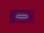
Figure 1: Left: Geometry two dimensional Sneddon test. Right: Geometrically locally refined mesh.

The fracture has a constant half length of $l_{0}=1.0$ and a varying width depending on the minimal element diameter. The parameters are given in Table 1.

Table 1: The setting of the material and numerical parameters for the Sneddon 2d test.

Parameter	Definition	Value
$\Omega$	Domain	$(-10,10)^{2}$
$h$	Diagonal cell diameter	test-dependent
$l_{0}$	Half crack length	$1.0$
$G_{C}$	Material toughness	$1.0$
$E$	Young’s modulus	$1.0$
$\mu$	Lamé parameter	$0.42$
$\lambda$	Lamé parameter	$0.28$
$\nu$	Poisson’s ratio	$0.2$
$p$	Applied pressure	$10^{-3}$
$l$	length scale parameter	$2h$
$\kappa$	Regularization parameter	$10^{-12}$
	Number of global refinements	$3-6$
$\operatorname{TOL}_{N}$	Tolerance outer Newton solver	$10^{-7}$

The quantities of interest in this test case are given by the so-called total crack volume

$$\operatorname{TCV}\coloneqq\int_{\Omega}u(x,y)\nabla\varphi(x,y)\,d(x,y)$$

and the crack opening displacement

$$\operatorname{COD}(x)\coloneqq[u\cdot n](x)\approx\int_{-\infty}^{\infty}u(x,y)\cdot\nabla\varphi(x,y)\,dy.$$

The analytical solutions [28] are given by

$$\operatorname{TCV}_{\operatorname{ref}}=\frac{2\pi\rho l_{0}^{2}}{E^{\prime}}$$

and

$$\operatorname{COD}_{\operatorname{ref}}=2\frac{pl}{E^{\prime}}\left(1-\frac{x^{2}}{l_{0}^{2}}\right)^{\frac{1}{2}}.$$

Table 2: The TCV-error on five different refinement levels and the average number of GMRES iterations over all incremental steps and Newton steps.

$h$	# DoFs	TCV	exact TCV	TCV-error [$\%$]	$\varnothing$ lin. iter.
$0.088$	$30669$	$0.00716698$	$0.0063186$	$18.8\%$	$2.96$
$0.044$	$62037$	$0.00650211$	$0.0063186$	$7.78\%$	$4.8$
$0.022$	$182325$	$0.00621216$	$0.0063186$	$2.99\%$	$16.13$
$0.011$	$653253$	$0.00607532$	$0.0063186$	$0.72\%$	$28.56$
$0.0055$	$2516661$	$0.00600751$	$0.0063186$	$0.4\%$	$50.97$

Figure 2: Visualization of the $\operatorname{COD}$-values for different $h$. The corresponding exact $\operatorname{TCV}$ values are given in Table 2.

In Table 2 and Figure 2, the results of the TCV and the COD on five different refinement levels are depicted and compared to the reference solution. We can clearly observe that the numerical solution tends to the reference solution under grid refinement.

References

- [1] L. Ambrosio and V. M. Tortorelli. Approximation of functional depending on jumps by elliptic functional via t-convergence. Comm. Pure Appl. Math, 43(8):999–1036, 1990.
- [2] L. Ambrosio and V. M. Tortorelli. On the approximation of free discontinuity problems. Boll. Un. Mat. Ital. B (7), 6(1):105–123, 1992.
- [3] D. Arndt, W. Bangerth, M. Feder, M. Fehling, R. Gassmöller, T. Heister, L. Heltai, M. Kronbichler, M. Maier, P. Munch, J.-P. Pelteret, S. Sticko, B. Turcksin, and D. Wells. The deal.II library, version 9.4. J. Numer. Math., 30(3):231–246, 2022.
- [4] B. Bourdin, G. A. Francfort, and J.-J. Marigo. Numerical experiments in revisited brittle fracture. J. Mech. Phys. Solids, 48(4):797–826, 2000.
- [5] J. Brown, V. Barra, N. Beams, L. Ghaffari, M. Knepley, W. Moses, R. Shakeri, K. Stengel, J. L. Thompson, and J. Zhang. Performance portable solid mechanics via matrix-free -multigrid, 2022.
- [6] T. C. Clevenger, T. Heister, G. Kanschat, and M. Kronbichler. A flexible, parallel, adaptive geometric multigrid method for FEM. ACM Trans. Math. Softw., 47(1):1–27, 2021.
- [7] D. Davydov, J. Pelteret, D. Arndt, M. Kronbichler, and P. Steinmann. A matrix-free approach for finite-strain hyperelastic problems using geometric multigrid. Int. J. Numer. Methods. Eng., 121(13):2874–2895, 2020.
- [8] G. Francfort and J.-J. Marigo. Revisiting brittle fracture as an energy minimization problem. J. Mech. Phys. Solids, 46(8):1319–1342, 1998.
- [9] M. Franco, J.-S. Camier, J. Andrej, and W. Pazner. High-order matrix-free incompressible flow solvers with GPU acceleration and low-order refined preconditioners. Comput. Fluids, 203:104541, 2020.
- [10] J.-L. Guermond, M. Kronbichler, M. Maier, B. Popov, and I. Toma. On the implementation of a robust and efficient finite element-based parallel solver for the compressible Navier-Stokes equations. Comput. Methods Appl. Mech. Eng., 389:114250, 2022.
- [11] T. Heister, M. F. Wheeler, and T. Wick. A primal-dual active set method and predictor-corrector mesh adaptivity for computing fracture propagation using a phase-field approach. Comput. Methods Appl. Mech. Engrg., 290:466–495, 2015.
- [12] S. Hüeber and B. Wohlmuth. A primal–dual active set strategy for non-linear multibody contact problems. Comput. Methods Appl. Mech. Engrg., 194(27):3147–3166, 2005.
- [13] B. Janssen and G. Kanschat. Adaptive Multilevel Methods with Local Smoothing for - and -Conforming High Order Finite Element Methods. SIAM Journal on Scientific Computing, 33(4):2095–2114, 2011.
- [14] D. Jodlbauer, U. Langer, and T. Wick. Matrix-free multigrid solvers for phase-field fracture problems. Comput. Methods Appl. Mech. Engrg., 372:113431, 2020.
- [15] D. Jodlbauer, U. Langer, and T. Wick. Parallel matrix-free higher-order finite element solvers for phase-field fracture problems. Math. Comp. Appl., 25(3):40, 2020.
- [16] D. Jodlbauer, U. Langer, T. Wick, and W. Zulehner. Matrix-free Monolithic Multigrid Methods for Stokes and Generalized Stokes Problems. SIAM Journal on Scientific Computing, 2024. accepted for publication.
- [17] L. Kolditz and K. Mang. On the relation of gamma-convergence parameters for pressure-driven quasi-static phase-field fracture. Ex. Count., 2:100047, 2022.
- [18] L. Kolditz, K. Mang, and T. Wick. A modified combined active-set newton method for solving phase-field fracture into the monolithic limit. Comput. Methods Appl. Mech. Engrg., 414:116170, 2023.
- [19] M. Kronbichler and K. Kormann. A generic interface for parallel cell-based finite element operator application. Computers & Fluids, 63:135–147, 2012.
- [20] M. Kronbichler and K. Kormann. Fast matrix-free evaluation of discontinuous Galerkin finite element operators. ACM Trans. Math. Softw., 45(3):1–40, 2019.
- [21] M. Kronbichler and K. Ljungkvist. Multigrid for matrix-free high-order finite element computations on graphics processors. ACM Trans. Parallel Comput., 6(1), 2019.
- [22] A. Mikelić, M. F. Wheeler, and T. Wick. Phase-field modeling through iterative splitting of hydraulic fractures in a poroelastic medium. GEM - International Journal on Geomathematics, 10(1), Jan 2019.
- [23] P. Munch, T. Heister, L. P. Saavedra, and M. Kronbichler. Efficient distributed matrix-free multigrid methods on locally refined meshes for FEM computations, 2022.
- [24] P. Munch, K. Kormann, and M. Kronbichler. hyper.deal: An efficient, matrix-free finite-element library for high-dimensional partial differential equations. ACM Trans. Math. Softw., 47(4):1–34, 2021.
- [25] A. Popp, M. W. Gee, and W. A. Wall. A finite deformation mortar contact formulation using a primal–dual active set strategy. Int. J. Numer. Meth. Engng., 79(11):1354–1391, 2009.
- [26] J. Schröder, T. Wick, S. Reese, and et al. A selection of benchmark problems in solid mechanics and applied mathematics. Arch. Comput. Methods Eng., 28(2):713–751, 2021.
- [27] B. Schröder and D. Kuhl. A semi-smooth Newton method for dynamic multifield plasticity. PAMM, 16(1):767–768, 2016.
- [28] I. N. Sneddon and M. Lowengrub. Crack problems in the classical theory of elasticity. SIAM Ser. Appl. Meth. John Wiley and Sons, Philadelphia, 1969.
- [29] M. Wichrowski and P. Krzyzanowski. A matrix-free multilevel preconditioner for the generalized stokes problem with discontinuous viscosity. Journal of Computational Science, 63:101804, 2022.
- [30] M. Wichrowski, P. Krzyżanowski, L. Heltai, and S. Stupkiewicz. Exploiting high-contrast stokes preconditioners to efficiently solve incompressible fluid-structure interaction problems, 2023.
- [31] T. Wick. Multiphysics Phase-Field Fracture: Modeling, Adaptive Discretizations, and Solvers, volume 28. Walter de Gruyter GmbH & Co KG, 2020.