Quantum aggregation with temporal delay

Abstract

Advanced quantum networking systems rely on efficient quantum error correction codes for their optimal realization. The rate at which the encoded information is transmitted is a fundamental limit that affects the performance of such systems. Quantum aggregation allows one to increase the transmission rate by adding multiple paths connecting two distant users. Aggregating channels of different paths allows more users to simultaneously exchange the encoded information. Recent work has shown that quantum aggregation can also reduce the number of physical resources of an error correction code when it is combined with the quantum multiplexing technique. However, the different channel lengths across the various paths means some of the encoded quantum information will arrive earlier than others and it must be stored in quantum memories. The information stored will then deteriorate due to decoherence processes leading to detrimental effects for the fidelity of the final quantum state. Here, we explore the effects of a depolarization channel that occurs for the quantum Reed-Solomon code when quantum aggregation involving different channel lengths is used. We determine the best distribution of resources among the various channels connecting two remote users. Further we estimate the coherence time required to achieve a certain fidelity. Our results will have a significant impact on the ways physical resources are distributed across a quantum network.

I Introduction

Future quantum networks will allow one to exchange information over large distances connecting multiple remote users Childress and Hanson (2013); Blok et al. (2015); Kimble (2008). This can be accomplished by sending high-quality quantum states, which can then be used for a variety of tasks, for instance, improving the security of the communication channels using quantum cryptographic protocols Bennett and Brassard (2014); Sangouard et al. (2011); Ekert (1991); Qiu (2014); Lo (1999); Hwang (2003); Munro et al. (2015), accelerating the computational time with quantum computers Nielsen and Chuang (2000); Bennett and DiVincenzo (2000); Devitt et al. (2013); Raussendorf and Briegel (2001); Knill (2005); Duan and Raussendorf (2005), and improving the precision of measurements with quantum sensing and imaging methods Dogen et al. (2017); Lugiato et al. (2002); Simon et al. (2014). However, due to the fragile nature of these quantum states errors and device imperfections will affect the performance of those approaches cancelling the advantages that these technologies have on their classical counterparts.

One method that allows the transmission of high fidelity states involves the use of quantum error correction (QEC) codes Ralph et al. (2005); Fowler et al. (2010a); Gottesman et al. (2001); Munro et al. (2012); Fowler et al. (2010b); Azuma et al. (2015); Mulidharan et al. (2014); Jiang et al. (2009). Information is now encoded in a more complex quantum system, which protect it from the errors occurring during transmission and recovered when needed. The complexity of such code requires a large number of physical resources for the encoding. Communication channels with low capacities Fanizza et al. (2020); Rosati et al. (2018); Shirokov (2017) and insufficient resources within a node will reduce the number of resources that can be transmitted over a single path, greatly affecting the communication rate. For instance, when several users are connected by the same path (or part of it), the number of channels of the path can be insufficient for an efficient communication between two users, decreasing thus their communication rate. Alternatively one can think of a single channel connecting two users. The communication rate, in this case, will be strictly limited by the repetition rate at which the photons are sent.

One way to alleviate these issues is to connect the users with more paths using quantum aggregation, in which the encoded states are distributed over the channels of those distinct paths Lo Piparo et al. (2020). In Lo Piparo et al. (2020) it was shown that using two paths for exchanging information using the quantum Reed-Solomon Grassl et al. (1999) (QRS) code leads to a drastic reduction of the transmittivity of the channels of that path while increasing only slightly the transmittivity of the other channels of the second path. Moreover, when higher-dimensional photonic encodings are used Lo Piparo et al. (2019) quantum aggregation shows a drastic reduction of the physical resources required to reach a threshold fidelity Lo Piparo et al. (2020). However, in the aggregation scenario a fundamental issue arises due to the different length of the two paths. In fact, part of the encoded information that arrives early at the remote site must be stored in a quantum memory, which will undergo a dephasing process affecting the final fidelity of the state ref . Once the delayed piece of encoded state reaches the far end, it can be used with the one retrieved from the quantum memory to correct the errors. The coherence time of the quantum memories used can play therefore a fundamental role in determining the performance of the QEC code when quantum aggregation is in use. A too large difference in the length of the two paths or a too short coherence time can be detrimental in recovering the information sent making the communication among users impossible. In this work we analyze the impact of temporal delays caused by the path length differences (i.e., the time interval in which a piece of an encoded quantum state is stored and that one in which it is retrieved) on the fidelity of the final decoded state in a quantum aggregation scenario. To this end, we consider two users that exchange information using the QRS code connected by two and three communication paths of different lengths. We determine the performance of such a system with delay for several configurations in which the information can be distributed and we determine the coherence times the quantum memories must have for an optimal performance.

The paper is divided as following: in Section II we analyze a quantum aggregation system applied to the smallest QRS code with a temporal delay in one path. Then in Section III we extend our analysis to higher dimensional QRS codes and show several different and interesting configuration arise. We conclude in Section IV.

II quantum aggregation with delay

Figure 1: Quantum aggregation over two paths of length $L_{2}>L_{1}$ containing each $N_{1},$ $N_{2}$ channels, respectively. Alice distributes her encoded state over the channels and send it through the two paths. Bob stores the received early qudits into quantum memories and decodes the state once the delayed qudits have arrived.

Let us begin by exploring the effect of temporal delay in quantum aggregation using the $[[n,1,d]]_{D}$ QRS code, where $n$ is the number of physical qudits of dimension $D$ used to encode one logical qudit and capable of correcting the loss of $d-1$ qudits, with $d$ being the code distance. In the general quantum aggregation scenario two users, Alice and Bob, are connected by two lossy paths having different length, $L_{1}$ and $L_{2},$ as shown in Fig. 1. In the following we assume that $D=n$ and $L_{2}>L_{1}$ with $N_{1}$ and $N_{2}$ being the number of channels inside path 1 and path 2, respectively ref . Alice encodes her state using a $[[n,1,d]]_{D}$ QRS code and distributes $N_{1}$ qudits in the channels of path 1 and $N_{2}$ qudits in the channels of path 2, respectively. We denoted such a configuration as $N_{1}+N_{2}.$ Then Bob decodes the received states if the number of the transmitted qudits arriving earlier ($N_{1}^{{}^{\prime}})$ is enough for retrieving the information sent by Alice ($N_{1}^{{}^{\prime}}\geq d)$, otherwise, when $N_{1}^{{}^{\prime}}<d$, he stores those qudits in quantum memories (QMs). We assume that the density matrix, $\rho,$ of these stored qudits undergo a depolarizing channel given by $\rho\rightarrow\rho^{\prime}=(1-p_{d})\rho+p_{d}I/D^{\prime},$ where $I$ is the $D^{\prime}$ dimensional identity operator and $p_{d}$ is the depolarization error probability given by $p_{d}=1-e^{-t/T_{2}},$ with $t=\left(L_{2}-L_{1}\right)/c$ and $T_{2}$ being the coherence time of the QMs. Next when $N_{1}^{{}^{\prime}}<d$ while the number of qudits transmitted over path 2 ($N_{2}^{{}^{\prime}})$ satisfies $N_{2}^{{}^{\prime}}\geq d,$ Bob uses the $N_{2}^{{}^{\prime}}$ qudits to recover the initial information discarding the stored qudits associated with the transmission through path $L_{1}.$ Now when both $N_{1}^{{}^{\prime}}<d$ and $N_{2}^{{}^{\prime}}<d$ but with $N_{1}^{{}^{\prime}}+N_{2}^{{}^{\prime}}\geq d$ Bob, retrieves the qudits stored into the QMs and applies a decoding procedure on all transmitted qudits. This latter case will affect the fidelity of the decoded state due to the $temporal$ $delay$ of the qudits traveling in path 2. Finally, when $N_{1}^{{}^{\prime}}+N_{2}^{{}^{\prime}}<d$ we assume for simplicity the state shared by Alice and Bob is a completely mixed state (the worst case) and all the information has been lost. We assume that the local gates errors are negligible compared to the memory depolarization errors.

Now let us explore the impact of the temporal delay in a quantum aggregation scenario using the smallest QRS code the $[[3,1,2]]_{3}$ code capable of correcting one error in which one logic qutrit is created using three physical qutrits. In the $[[3,1,2]]_{3}$ QRS code protocol Alice encodes her initial qutrit $\left.|\psi\right\rangle_{A}=\left.\alpha_{0}|0\right\rangle+\left.\alpha_{1}|1\right\rangle+\left.\alpha_{2}|2\right\rangle$ into the logic state $\left.|\psi\right\rangle_{L}=\left.\alpha_{0}|0\right\rangle_{L}+\left.\alpha_{1}|1\right\rangle_{L}+\left.\alpha_{2}|2\right\rangle_{L},$ where $\left.|0\right\rangle_{L}=\left(\left.|000\right\rangle+\left.|111\right\rangle+\left.|222\right\rangle\right)/\sqrt{3};$ $\left.|1\right\rangle_{L}=\left(\left.|012\right\rangle+\left.|120\right\rangle+\left.|201\right\rangle\right)/\sqrt{3}$ and $\left.|2\right\rangle_{L}=\left(\left.|021\right\rangle+\left.|102\right\rangle+\left.|210\right\rangle\right)/\sqrt{3}.$ She sends this encoded state over a lossy path to Bob. Upon a successful transmission of the state sent by Alice, Bob applies a decoding procedure described in Muralidharam et al. (2017) to retrieve the initial state. In the quantum aggregation scenario, we have two configurations; the $2+1$ configuration and the $1+2$ configuration, in which $2(1)$ qudits are traveling in the channels of path 1 having a transmissivity $p_{1}=e^{-L_{1}/L_{\mathrm{att}}}$ while $1(2)$ qutrits are sent via path 2 with transmission probability $p_{2}=e^{-L_{2}/L_{\mathrm{att}}},$ respectively. Here $L_{\mathrm{att}}=22$ km is the attenuation length of the optical fiber channels.

In the 2+1 configuration the fidelity, $F_{2+1},$ of the state received and decoded by Bob is

$$F_{2+1} =p_{1}^{2}p_{2}+2p_{1}p_{2}(1-p_{1})\left(1-\frac{2}{3}p_{d}\right)$$ (1)

$$+p_{1}^{2}(1-p_{2})+(1-P_{s_{1}})/27$$

where $P_{s_{1}}=p_{1}^{2}p_{2}+2p_{1}p_{2}(1-p_{1})+p_{1}^{2}(1-p_{2})$ is the probability of the successful transmission of information from Alice to Bob. Let us give an intuitive derivation of Eq. (1) that can be easily extended to derive the fidelity of higher dimensional QRS codes. The no-loss term, which is the first and dominant term in Eq. (1), and the loss of the qudit traveling in path 2 (third term in Eq. (1)) do not depend on the depolarization error $p_{d}$ because Bob applies immediately the decoding procedure on the two qutrits traveling in the channels of path 1. Then, in the case in which one of the two qudits traveling in path 1 is lost, the temporal delay due to the storage of the transmitted qudit contributes to the fidelity with a term proportional to $\left(1-\frac{2}{3}p_{d}\right),$ which has been derived in Appendix A. To gain an understanding of the behavior of the fidelity we plot in Fig. 2(a) the fidelity $F_{2+1}$ versus the memories coherence time for $L_{1}=1$ km and $L_{2}=3$ km (solid blue curve). We see that the coherence time of the QM only affects the fidelity when $T_{2}<0.1$ ms and noting that for no memory $(T_{2}=0)$ $F_{2+1}\sim 0.94.$ This is due to the fact that the the no-loss term does not depend on $p_{d}.$ Therefore, even when there are no QMs in the system the transmitted state can be used to extract some information. A similar explanation can be given to the case in which $L_{2}\rightarrow\infty,$ (see the left graph of the inset of Fig. 2(a)). Here we plot the fidelity versus $L_{2}$ with $L_{1}=1$ km for $T_{2}=$ 1 ms (blue curve), $T_{2}=$ 0.1 ms (red curve) and $T_{2}=0.01$ ms, respectively. We observe that the fidelity decreases at lower coherence times while reaching an asymptotic value of $\sim 0.92$ at large values of $L_{2},$ from which information can partially be extracted. This can be explained considering that, for this configuration, the no-loss term corresponds to the case in which two qudits are successfully transmitted and one is lost with very high probability. Therefore, since this code can correct the loss of one qudit, the transmitted state containing two qudits with probability ($\sim p_{1}^{2})$, still has sufficient information sallowing the fidelity to exceed $50\%.$

The alternate 1+2 configuration changes quite drastically. It is straight forward to show that $F_{1+2}$ is

$$F_{1+2} =p_{2}^{2}p_{1}+2p_{1}p_{2}(1-p_{2})\left(1-\frac{2}{3}p_{d}\right)$$ (2)

$$+p_{2}^{2}(1-p_{1})+(1-P_{s_{2}})/27$$

where $P_{s_{2}}=p_{2}^{2}p_{1}+2p_{1}p_{2}(1-p_{2})+p_{2}^{2}(1-p_{1}).$ Even in this configuration the dominant term is the no-loss term, which does not depend on $p_{d}$ because, although the two qudits arrive later, they can be immediately be used to decode the state while discarding the early qudit transmitted over the path 1. The second term in Eq. (2) refers to the lost of a qudit traveling in path 2. Therefore, Bob needs to retrieve the stored qudit from the QM to decode the state together with the single qudit transmitted over path 2. The contribution to the fidelity from the depolarization channel applied to the stored qudit is equal to the previous configuration. Finally, the third term in Eq. (2) does not depend on $p_{d}$ because Bob can use the two qudits transmitted over path 2 to decode the state. To visualize this we plot $F_{2+1}$ (solid red line) versus $T_{2}$ at the same numerical values of the previous configuration, as shown in Fig. 2(a). As expected, the fidelity in this case has much lower values because the no-loss term suffers the loss of two qudits with higher probability, hence the second term in Eq. (2) is more relevant in this case. In other words the coherence time in this case affect the fidelity more than the other case. This can also be seen from the graph in the right side of the inset of Fig. 2(a). Here, we plot the fidelity versus $L_{2}$ for different coherence times. In this case the probability of losing two qudits traveling in path 2 increases with $L_{2},$ (mathematically, the first term in Eq. (2) decreases), hence, the contribution to the fidelity from the second term is more significant. In this case one can see that $T_{2}$ determines a threshold value for $L_{2}$ after which the fidelity is below $50\%$ (see the crossing points of the curves with the $x$ axis in the graph in the right side of the inset of Fig. 2(a)). From this considerations we conclude (as expected) that distributing more qudits in the shorter channel gives a significant advantage in terms of having higher fidelities and being slightly affected by the coherence time. Please see Appendix B for the full derivation of Eq. (1) and (2).

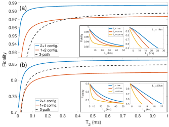
Figure 2: Fidelity of the decoded state received by Bob versus the coherence time, $T_{2},$ of the QM used to store the qutrits transmitted through path 1, in the 2+1 configuration (solid blue lines) and 1+2 configuration (solid red lines) for (a) $L_{1}=1$ km, $L_{2}=3$ km and (b) $L_{1}=5$ km, $L_{2}=8$ km. In the insets we depict the fidelity versus $L_{2}$ at (a) $L_{1}=1$ km and (b) $L_{1}=5$ km for both configurations. Also shown for the 3-path configuration as the black dashed curves (a) with $L_{1}=1$ km, $L_{2}=2$ km, $L_{3}=3$ km and (b) with $L_{1}=5$ km, $L_{2}=6$ km, $L_{3}=8$ km.

We expect that for higher values of $L_{1}$ all the results described above are worse for both configurations. This scenario is shown in Fig. 2(b), where we plot the fidelities of the configurations versus $T_{2}$ at $L_{1}=5$ km and $L_{2}=$ 8 km and in the inset where we plot the fidelities of both configurations versus $L_{2}$ at $L_{1}=5$ km. Even in this case the fidelity in the $2+1$ configuration reaches an asymptotic value as $L_{2}$ increases, which is much lower than the previous case.

It is interesting now to add one more path (path 3), with transmission probability $p_{3}=e^{-L_{3}/L_{\mathrm{att}}},$ to the previous scheme, such that $L_{3}>L_{2}>L_{1}$ while maintaining the same highest distance separating Alice and Bob. In this case, each qutrit travels across a channel in the corresponding path. This can be referred to as the 1+1+1 configuration. The fidelity of Bob’s decoded state is

$$\begin{array}[]{c}\begin{aligned} F_{1+1+1}&=p_{1}p_{2}p_{3}\left(1-\frac{2}{3}p_{d_{12}}\right)\\ &+p_{2}p_{3}(1-p_{1})\left(1-\frac{2}{3}p_{d_{23}}\right)\\ &+p_{1}p_{3}(1-p_{2})\left(1-\frac{2}{3}p_{d_{13}}\right)\\ &+p_{1}p_{2}(1-p_{3})\left(1-\frac{2}{3}p_{d_{12}}\right)\\ &+(1-P_{s})1/27,\end{aligned}\end{array}$$ (3)

where $p_{d_{ij}}=1-e^{-T_{ij}/T_{2}},$ with $T_{ij}=|L_{i}-L_{j}|/c$ and $P_{s}=p_{1}p_{2}p_{3}+p_{2}p_{3}(1-p_{1})+p_{1}p_{3}(1-p_{2})+p_{1}p_{2}(1-p_{3}).$ In this case, the no-loss term of Eq. (3) depends on $p_{d}$ because the qutrit traveling in the channel of path 1 arrives first and needs to be stored in a QM before Bob can apply a decoding process with a second qudit. One can also see that all the other terms in Eq. (3) depends on $p_{d}$ because in the loss event of any qudit, Bob needs to wait for another one to start the decoding process. Figure 2(a) shows the fidelity of Eq. (3) (black dashed line) at $L_{1}=1$ km, $L_{2}=2$ km and $L_{3}=3$ km. One can see that for small values of $T_{2}$ ($T_{2}<0.1$ ms) the no loss term greatly affects the fidelity whereas for higher values of $T_{2}$ the fidelity of the 3-path case increases until it crosses the 1+2 configuration of the 2-path case at a crossing point $T_{2}^{c}\simeq 0.3$ ms. This is due to the fact that the expression of the fidelity of the state received by Bob in the 3-path case is more affected by the coherence time than $1+2$ case as one can see comparing Eq. (1) with Eq. (3). Therefore we expect that for large values of $T_{2}$ the no-loss term of Eq. (3) becomes higher than the no-loss term of Eq. (1) because when $T_{2}\rightarrow\infty$ the qudit in path 2 travels over a smaller distance than the qudits of the 1+2 configuration. At $L_{1}=5$ km and $L_{2}=8$ km the 3-path case has also a lower fidelity as shown from the dashed curve in Fig. 2(b). However, in this case the crossing point of this curve with the one corresponding to the $1+2$ configuration is slightly lower than the crossing point shows in Fig. 2(a). This can be explained by considering that for larger distances the main source of error is the channel loss, hence, the coherence time affects less the fidelity of the decoded state. In fact we can see that at very low values of $T_{2}$ the fidelity of the 3-path case is very similar to the $1+2$ case.

III temporal delay for higher dimensional codes

So far we have considered the smallest QRS code that can correct 1 loss errors. What happens as we increase the code size? We analyze the effects of the temporal delay in a quantum aggregation scenario for the $[[5,1,3]]_{5}$ and the $[[7,1,4]]_{7},$ QRS codes, which can fix the loss of 2 and 3 qudits, respectively. Let us begin with the $[[5,1,3]]_{5}$ code. Here there are 4 possible configurations: 4+1, 3+2, 2+3 and 1+4.

III.1 The 4+1 and 1+4 configurations

In these configurations for the $[[5,1,3]]_{5}$ code, the fidelity of the state decoded by Bob is:

$$\begin{array}[]{c}\begin{aligned} F_{4+1}&=p_{1}^{4}p_{2}+4p_{1}^{3}p_{2}(1-p_{1})+p_{1}^{4}(1-p_{2})+\\ &+6p_{1}^{2}p_{2}(1-p_{1})^{2}f_{1}(p_{d})\\ &+4p_{1}^{3}(1-p_{1})(1-p_{2})+(1-P_{s_{1}})/5^{5}\end{aligned}\end{array}$$ (4)

and

$$\begin{array}[]{c}\begin{aligned} F_{1+4}&=p_{2}^{4}p_{1}+4p_{2}^{3}p_{1}(1-p_{2})+p_{2}^{4}(1-p_{1})\\ &+6p_{2}^{2}p_{1}(1-p_{2})^{2}f_{2}(p_{d})\\ &+4p_{2}^{3}(1-p_{2})(1-p_{1})+(1-P_{s_{2}})/5^{5}.\end{aligned}\end{array}$$ (5)

where $P_{s_{1(2)}}=p_{1(2)}^{4}p_{2(1)}+4p_{1(2)}^{3}p_{2(1)}(1-p_{1(2)})+p_{1(2)}^{4}(1-p_{2(1)})+6p_{1(2)}^{2}p_{2(1)}(1-p_{1(2)})^{2}+4p_{1(2)}^{3}(1-p_{1(2)})(1-p_{2(1)})$ and $f_{1(2)}(p_{d})$ being a contribution to the fidelity when 2 or 1 qudits are dephasing, respectively.

Comparing Eq. (4) with Eq. (5) one can see that the expressions of the two fidelities are almost identical except for the 4th term, which is multiplied by $f_{1,2}(p_{d}),$ respectively, whose analytical expression is given in Appendix B. What however is important is that $f_{1}(p_{d})\leq f_{2}(p_{d})$ and only equal at $p_{d}=0,$ $1.$ This is due to the fact that the term $f_{1}(p_{d})$ can be considered as the fidelity of a density matrix in which 2 qudits are dephasing whereas $f_{1}(p_{d})$ takes into account the dephasing of a single qudit. Hence in this latter case, less information has been lost. However, the dominant term in both Eq. (4) and Eq. (5) is the no-loss term, hence,

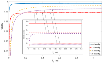
Figure 3: Fidelity of the state decoded by Bob when Alice encodes her state using the $[[5,1,3]]_{5}$ QRS code in a quantum aggregation scenario for $L_{1}=$ 1 km and $L_{2}=3$ km. The blue solid curve (red dash-dotted curve) refers to the 4+1 (1+4) configuration in which Alice distribute four (one) qudits into the shorter channels and one (four) qudits in the longer channels, respectively, whereas the dashed yellow curve (dotted purple curve) refers to the 3+2 configuration in which Alice distributes three (two) qudits into the shorter channels and three(two) qudits in the longer ones respectively. In the inset, we plot the contributions to the fidelity of the probability of losing zero (solid curves), one (dashed curves) and two (dotted curves) qudits for the 1+4 and 2+3 configurations.

$F_{1}$ is higher than $F_{2}$ for any value of the dephasing time $T_{2},$ as shown in Fig. Fig. 3. Therefore it is more advantageous to distribute more qudits into the shorter path as well as we obtained for the three dimensional code.

III.2 The 3+2 and 2+3 configurations

It is now interesting to analyze the 3+2 and 2+3 configurations of the $[[5,1,3]]_{5}$ QRS code. The respective fidelities are

$$\begin{array}[]{c}\begin{aligned} F_{3+2}&=p_{1}^{3}p_{2}^{2}+3p_{1}^{2}p_{2}^{2}(1-p_{1})f_{3}(p_{d})+2p_{1}^{3}p_{2}(1-p_{2})\\ &+3p_{1}p_{2}^{2}(1-p_{1})^{2}f_{2}(p_{d})+p_{1}^{3}(1-p_{2})^{2}\\ &+6p_{1}^{2}p_{2}(1-p_{1})(1-p_{2})f_{1}(p_{d})+(1-P_{s_{1}})/5^{5}\end{aligned}\end{array}$$ (6)

and

$$\begin{array}[]{c}\begin{aligned} F_{2+3}&=p_{2}^{3}p_{1}^{2}+3p_{2}^{2}p_{1}^{2}(1-p_{2})f_{3}(p_{d})+2p_{2}^{3}p_{1}(1-p_{1})\\ &+3p_{2}p_{1}^{2}(1-p_{2})^{2}f_{1}(p_{d})+p_{2}^{3}(1-p_{1})^{2}\\ &+6p_{2}^{2}p_{1}(1-p_{2})(1-p_{1})f_{2}(p_{d})+(1-P_{s_{2}})/5^{5},\end{aligned}\end{array}$$ (7)

where $P_{s}=p_{1(2)}^{3}p_{2(1)}^{2}+3p_{1(2)}^{2}p_{2(1)}^{2}(1-p_{1(2)})+2p_{1(2)}^{3}p_{2(1)}(1-p_{2(1)})+3p_{1(2)}p_{2(1)}^{2}(1-p_{1(2)})^{2}+p_{1(2)}^{3}(1-p_{2(1)})^{2}+6p_{1(2)}^{2}p_{2(1)}(1-p_{1(2)})(1-p_{2(1)}).$

Figure 3 shows that, even in this configuration, it is more convenient to use more qudits in the shorter path. In fact, $F_{1}$ (dashed yellow curve) is higher than $F_{2}$ (dotted purple curve) for any value of $T_{2}.$ Further, Fig. 3 shows that at $T_{2}\geq 0.16$ ms the fidelity of the $2+3$ configuration outperforms the fidelity of the $1+4$ configuration. This can be explained with the fact that some terms of Eq. (7) are much more affected by the dephasing channel than Eq. (5). In fact, in the inset of Fig. 3 we plot for those two configurations, the contributions to the fidelity coming from the probability of losing zero (solid curves), one (dashed curves) and two (dotted curves) qudits. We expect that that for large values of $T_{2}$ the probability of not losing any qudit is higher in the 2+3 configuration (purple solid curve of the inset) because less qudits are traveling in the longer channel compared to the 1+4 configuration (red solid curve of the inset) whereas the loss terms must be smaller. On the other hand, at lower values of $T_{2}$, the contribution of losing one qudit for the 2+3 configuration is strongly affected by dephasing whereas the one of the 1+4 configuration does not depend on it. As regards the probability of losing two qudits, the dephasing channel affects both configurations with the 2+3 being slightly lower.

III.3 The $[[7,1,4]]_{7}$ QRS code

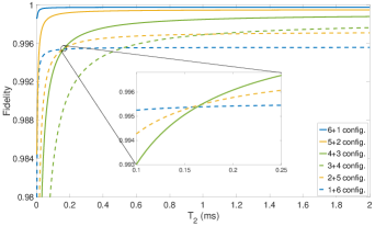
Figure 4: Fidelity of the state received by Bob when Alice encodes her state using the $[[7,1,4]]_{7}$ QRS code in a quantum aggregation scenario for $L_{1}=1$ km and $L_{2}=3$ km. The blue solid curve (blue dashed curve) refers to the 6+1 (1+6) configuration in which Alice distribute six (one) qudits into the shorter channels and one (six) qudits in the longer channels, respectively; the solid yellow curve (dashed yellow curve) refers to the 5+2 configuration in which Alice distribute five (two) qudits into the shorter channels and two (five) qudits in the longer ones, respectively; the solid green curve (dashed green curve) refers to the 4+3 configuration in which Alice distribute four (three) qudits into the shorter channels and three (four) qudits in the longer ones, respectively. In the inset we plot the portion of the graph in which the 1+6, 2+5 and 4+3 configurations cross.

In this subsection we show the results of the $[[7,1,4]]_{7}$ QRS code. The analytical expression of the fidelities for all possible configurations are listed in Appendix C. Figure 4 shows the fidelities of all configurations of the $[[7,1,4]]_{7}$ QRS code, where the solid curves refer to the case in which a higher number of qudits travel in the shorter channels whereas the dashed curves refer to the case in which the smaller number of qudits travel in longer channels. One can notice the following common features shared with the $[[5,1,3]]_{5}$ QRS case illustrated above. Firstly the case in which more qudits travel in the shorter path has higher fidelity than the other case for any value of $T_{2}.$ This is mainly due to the contribution of the no-loss term, which is the dominant term in the expressions of the fidelities. Then, when the qudits are almost equally distributed between the two channels (for instance the 3+2 configuration of the $[[5,1,3]]_{5}$ QRS code, or the 4+3 configuration of the $[[7,1,4]]_{7}$ QRS code) the fidelities are much more affected by the dephasing. As a consequence, these fidelities will reach the asymptotic limit of $T_{2}\rightarrow\infty$ at higher values of $T_{2}$ as shown in Fig. 4 (for instance, the purple curve in Fig. 3 and the green curves in Fig. 4). Then, as well as the this case of the $[[5,1,3]]_{5}$ QRS code, there is a crossing point in which the fidelities of different configurations intersect. The inset of Fig. 4 shows that this dephasing crossing point, $T_{2}^{c},$ occurs at $T_{2}^{c}=0.16$ ms. This can be explained with a very similar motivation given in the $[[5,1,3]]_{5}$ QRS code case. In fact, the loss terms in the fidelity’s expressions of the configurations in which the qudits are more evenly distributed depend on the dephasing channel much more than the loss terms of the uneven distributions, as one can see in Eqs. (14) - (16) compared to Eq. (12). Hence, the corresponding fidelities assume high values at $T_{2}\rightarrow\infty$ and very low values at $T_{2}\rightarrow 0$ for the even distribution cases leading to a crossing point with the fidelity of the uneven case. This is an interesting feature of the aggregation network because one user can achieve a faster communication rate, sending more qudits simultaneously the more even is the distribution, while having better fidelities than the more uneven distribution case for certain values of $T_{2}.$ On the other hand, when the highest value of fidelity is required, then a more uneven distribution is preferred. This aspect can play an important role for some quantum communication systems in which a trade-off between fidelity of the transmitted states and transmission rate is the key factor, such as in several quantum key distribution schemes Ekert (1991); Lo (1999); Hwang (2003); Qiu (2014).

IV Conclusion and discussion

Distributing physical resources over multiple channels of different length in a quantum aggregation scenario will require the use of quantum memories to store the states arriving earlier. The decoherence process occurring in the memories will partially destroy the stored information before the delayed state arrives. Here we analyze the effect of such a delay time in a QRS code having dimension three, five and seven, respectively. For these codes, we analytically calculate the fidelity of the final state as function of the channel loss and the dephasing time for different configurations in which the resources are evenly or unevenly distributed over two paths of different length. We obtain that for a coherence times $T_{2}>1$ ms the fidelities of all the configurations asymptotically reach their optimal value. This threshold for the coherence time is vastly reachable with today’s technology using, for instance, ion qubits Wang et al. (2021), superconducting cavities Milul et al. (2023), nuclear qubits of NV centers Nemoto et al. (2016) and ensemble-based quantum memories Chen et al. (2016). We also analyze the behavior of such fidelities at a fixed value of the coherence time when the length difference between the two paths increases. In this case we obtain an asymptotic value for the fidelity when the majority of the qudits travels across the shorter path regardless the value of the coherence time.

On the other hand, when most of the qudits travel in the longer path we determine the largest achievable distance of such a path, which is strongly affected by the coherence time. We show that while quantum aggregation allows users in a quantum network to exchange information faster, the impact of a temporal delay in the received states can have a detrimental effect on the quality of the transmitted information. The secret key bit rate can be a good figure of merit to estimate the performance of a quantum network since it takes into account both the repetition rate at which bits are shared between two remote parties as well as the quality of the density matrix shared by them. Optimizing the secret key rate using quantum aggregation can therefore be a valid route to follow for the evaluation of the performance of tomorrow’s quantum networks. Besides the configurations analyzed in this work can potentially provide a guideline on the architecture of quantum networks. Future works might consider using other error correction codes with quantum aggregation due to its versatility as well as adding more paths connecting users.

Appendix A Decoding procedures

In this Appendix we illustrate the procedure to recover the state sent by Alice for the $[[5,1,3]]_{5}$ and $[[7,1,4]]_{7}$ QRS codes, respectively, in a lossy channel. Figure 5 shows the circuit that Bob applies to the encoded state sent by Alice when (a) illustrates the situation involving the loss of a single qudit and (b) the loss of two qudits. The gates represent a sum modulo $5$ between two qudits of dimension $5.$ After these gates are applied the remaining qudits except the first one are measured in the computational basis. These measurements will ideally project the first qudit into the state $\left.|\psi\right\rangle_{A}=\alpha_{0}\left.|0\right\rangle+\alpha_{1}\left.|1\right\rangle+\alpha_{2}\left.|2\right\rangle+\alpha_{3}\left.|3\right\rangle+\alpha_{4}\left.|4\right\rangle.$ Similarly, it is possible to retrieve the initial state of Alice for the $[[7,1,4]]_{7}$ QRS code with the decoding circuits shown in Fig. 6(a, b, c), which correspond to the loss of one, two and three qudits, respectively.

Appendix B Fidelities after dephasing

Figure 5: Decoding circuit of the $[[5,1,3]]_{5}$ QRS code when (a) one qudit and (b) two qudits are lost, respectively. The dashed lines refer to the loss of a qudit. The symbol “+” refers to the sum mod 5 gate.

Figure 6: Decoding circuit of the $[[7,1,4]]_{7}$ QRS code when (a) one qudit, (b) two qudits and (c) three qudits are lost, respectively. The dashed lines refer to the loss of a qudit. The symbol “+” refers to the sum mod 7 gate.

Here, we derive the general approach we use to calculate the fidelity of the $[[3,1,2]]_{3}$ QRS code when the density matrix of the state undergoes a dephasing channel. We then derive the terms that depend on the dephasing for the $[[5,1,3]]_{5}$ and $[[7,1,4]]_{7}$ QRS codes.

Alice initially encodes her physical state $\left.|\psi\right\rangle_{A}=\alpha_{0}\left.|0\right\rangle+\alpha_{1}\left.|1\right\rangle+\alpha_{2}\left.|2\right\rangle$ into the logical state $\rho_{L}=\left.|\psi\right\rangle_{L}\left\langle\psi|_{L}\right.$ and sends it to Bob over lossy channels, having transmission probability $p_{1}$ and $p_{2},$ respectively. After the channel loss, the mixed density matrix can be expressed as a sum of density matrices multiplied by the loss probability, i.e.,:

$$\begin{array}[]{c}\begin{aligned} \rho_{L}\rightarrow\rho^{\prime}&=p_{1}^{2}p_{2}\rho_{0}+p_{1}p_{2}(1-p_{1})\rho_{1}+p_{1}p_{2}(1-p_{1})\rho{}_{2}\\ &+p_{1}^{2}(1-p_{2})\rho_{3}+(1-P_{s})I_{3}\end{aligned}\end{array}$$ (8)

where $\rho_{0},$ $\rho_{1},$ $\rho_{2}$ and $\rho_{3}$ are the density matrices resulting from the loss of no qudit, the first qudit, the second or the third qudit, respectively, while $I_{3}$ is the normalized identity operator of the Hilbert space spanned by the three qudits. We assume that the terms of the density matrix $\rho^{{}^{\prime}}$ corresponding to the loss of two and three qudits are given by $I_{3}.$ The fidelity of the state given by Eq. (8) is therefore a lower bound of the total fidelity. Now, the density matrices, $\rho_{1}$ and $\rho_{2},$ undergo to a depolarization channel given by $\rho_{1,2}\rightarrow\rho^{\prime}_{1,2}=(1-p_{d})\rho_{1,2}+p_{d}I_{1,2}Tr_{12}\left(\rho_{1,2}\right),$ where $I_{1,2}$ is the identity of the Hilbert space spanned by qudit 1 and 2, respectively. Substituting $\rho^{\prime}_{1,2}$ in Eq. (8) we obtain:

$$\begin{array}[]{c}\begin{aligned} \rho^{\prime}\rightarrow\rho(p_{d})&=p_{1}^{2}p_{2}\rho_{0}+p_{1}p_{2}(1-p_{1})\rho^{\prime}_{1}\\ &+p_{1}p_{2}(1-p_{1})\rho^{\prime}_{2}+p_{1}^{2}(1-p_{2})\rho_{3}+(1-P_{s})I_{3}.\end{aligned}\end{array}$$ (9)

Bob applies the decoding procedure described in Muralidharam et al. (2017), which ideally restore the initial state of Alice $\left.|\psi\right\rangle_{A}.$ The fidelity, $F,$ is given by $F=_{A}\left\langle\psi|\rho(p_{d})\left.|\psi\right\rangle_{A}.\right.$

We now sh ow the derivation of the term $f_{1}(p_{d})$ of Eq. 4. To this end, let us assume that the encoded state of the $[[5,1,3]]_{5}$ QRS code losses the first two qudits. The resulting state is then given by $\rho_{l}=\sum_{i=0}^{5}\left.|\psi\right\rangle_{i}\left\langle\psi|_{i},\right.$ where

$\begin{aligned} \left.|\psi\right\rangle_{0}&\text{$\left.\,=\alpha_{0}|000\right\rangle$+$\left.\alpha_{1}|341\right\rangle$+$\left.\alpha_{2}|132\right\rangle$+$\left.\alpha_{3}|423\right\rangle$}+\left.\alpha_{4}|214\right\rangle,\\ \left.|\psi\right\rangle_{1}&=\left.\alpha_{0}|111\right\rangle+\left.\alpha_{1}|402\right\rangle+\left.\alpha_{2}|243\right\rangle+\left.\alpha_{3}|034\right\rangle+\left.\alpha_{4}|320\right\rangle,\\ \left.|\psi\right\rangle_{2}&=\left.\alpha_{0}|222\right\rangle+\left.\alpha_{1}|013\right\rangle+\left.\alpha_{2}|304\right\rangle+\left.\alpha_{3}|140\right\rangle+\left.\alpha_{4}|431\right\rangle,\\ \left.|\psi\right\rangle_{3}&=\left.\alpha_{0}|333\right\rangle+\left.\alpha_{1}|124\right\rangle+\left.\alpha_{2}|410\right\rangle+\left.\alpha_{3}|201\right\rangle+\left.\alpha_{4}|042\right\rangle,\\ \left.|\psi\right\rangle_{4}&=\left.\alpha_{0}|444\right\rangle+\left.\alpha_{1}|230\right\rangle+\left.\alpha_{2}|021\right\rangle+\left.\alpha_{3}|312\right\rangle+\left.\alpha_{4}|103\right\rangle.\end{aligned}$

We now apply a depolarization channel to $\rho_{l}$ and we obtain $\rho_{l}\rightarrow\rho^{\prime}_{l}=(1-p_{d})^{2}\rho_{l}+p_{d}(1-p_{d})I_{1}Tr_{1}(\rho_{l})+p_{d}(1-p_{d})I_{2}Tr_{2}(\rho_{l})+p_{d}^{2}I_{12}Tr_{12}(\rho_{l})$, where $I_{1(2)}$ is the identity operator of the Hilbert space spanned by the qudit 1(2) and $I_{12}=I_{1}\otimes I_{2}.$ Bob will apply the decoding procedure of Fig. 5 to the state $\rho^{\prime}_{l}$ obtaining a decoded state $\rho^{\prime\prime}_{l}$. The contribution of $\rho^{\prime\prime}_{l}$ to the fidelity of Eq. (4), $f_{1}(p_{d})$ will be:

$$\begin{array}[]{c}\begin{aligned} f_{1}(p_{d})&=_{A}\left\langle\psi|\rho^{\prime\prime}_{l}\left.|\psi\right\rangle_{A}=\right.\left\langle\psi|_{A}\rho(p_{d})\left.|\psi\right\rangle_{A}\right.\\ &=\frac{1}{20(\frac{5}{4}-2p_{d}+p_{d}^{2})}\left[4\left(4\sum_{i=0}^{4}\alpha_{i}^{4}+13\sum_{i,j=0}^{4}\alpha_{i}^{2}\alpha_{j}^{2}\right)p_{d}^{2}\right.\\ &\left.-20\left(2\sum_{i=0}^{4}\alpha_{i}^{4}+5\sum_{i,j=0}^{4}\alpha_{i}^{2}\alpha_{j}^{2}\right)p_{d}+25\right].\end{aligned}\end{array}$$ (10)

It is straightforward to see that $f_{1}(p_{d})$ has a minimum at $\alpha_{0}=\alpha_{1}=\alpha_{2}=\alpha_{3}=\alpha_{4}=1/\sqrt{5}$ , which is the numerical value we have used to find the fidelities of Eq. (4) and (5). The derivation of all the other terms due to dephasing follow a similar approach, hence, we only give here the final result:

$f_{2}(p_{d})=\frac{1}{5-4p_{d}}\left[5-2\left(2\sum_{i=0}^{4}\alpha_{i}^{4}+5\sum_{i,j=0}^{4}\alpha_{i}^{2}\alpha_{j}^{2}\right)p_{d}\right],$

$\begin{array}[]{c}\begin{aligned} f_{3}(p_{d})&=\frac{1}{(5-4p_{d})^{2}}\left[2\left(8\sum_{i=0}^{4}\alpha_{i}^{4}+25\sum_{i,j=0}^{4}\alpha_{i}^{2}\alpha_{j}^{2}\right)p_{d}^{2}\right.\\ &\left.-20\left(2\sum_{i=0}^{4}\alpha_{i}^{4}+5\sum_{i,j=0}^{4}\alpha_{i}^{2}\alpha_{j}^{2}\right)p_{d}+25\right]\end{aligned}\end{array}.$ The contributions to the fidelity that depend on $p_{d}$ of the $[[7,1,4]]_{7}$ QRS code are:

$\begin{array}[]{c}\begin{aligned} g_{1}(p_{d})&=\frac{342(\frac{7}{6}-p_{d})}{7(49-30p_{d}^{3}+108p_{d}^{2}-126p_{d})}\left[\frac{2}{19}\left(6\sum_{i=0}^{4}\alpha_{i}^{4}\right.\right.\\ &\left.+19\sum_{i,j=0}^{4}\alpha_{i}^{2}\alpha_{j}^{2}\right)p_{d}^{2}-42\left(2\sum_{i=0}^{4}\alpha_{i}^{4}\right.\\ &\left.+5\sum_{i,j=0}^{4}\alpha_{i}^{2}\alpha_{j}^{2}p_{d}+\frac{49}{57}\right],\end{aligned}\end{array}$

$g_{2}(p_{d})=\frac{1}{6\left(\frac{7}{6}-p_{d}\right)}\left[7-2\left(3\sum_{i=0}^{4}\alpha_{i}^{4}+7\sum_{i,j=0}^{4}\alpha_{i}^{2}\alpha_{j}^{2}\right)p_{d}\right],$

$\begin{array}[]{c}\begin{aligned} g_{3}(p_{d})&=\frac{1}{(6p_{d}-7)^{3}}\left[2\left(108\sum_{i=0}^{4}\alpha_{i}^{4}+343\sum_{i,j=0}^{4}\alpha_{i}^{2}\alpha_{j}^{2}\right)p_{d}^{3}\right.\\ &-42\left(18\sum_{i=0}^{4}\alpha_{i}^{4}+49\sum_{i,j=0}^{4}\alpha_{i}^{2}\alpha_{j}^{2}\right)p_{d}^{2}\\ &\left.+294\left(3\sum_{i=0}^{4}\alpha_{i}^{4}+7\sum_{i,j=0}^{4}\alpha_{i}^{2}\alpha_{j}^{2}\right)p_{d}-343\right],\end{aligned}\end{array}$

$\begin{aligned} g_{4}(p_{d})&=\frac{1}{(49-35p_{d}+49p_{d}^{2})}\left[p_{d}^{2}-7\left(5\sum_{i=0}^{4}\alpha_{i}^{4}\right.\right.\\ &\left.\left.+14\sum_{i,j=0}^{4}\alpha_{i}^{2}\alpha_{j}^{2}\right)p_{d}+49\right],\end{aligned}$

$\begin{array}[]{c}\begin{aligned} g_{5}(p_{d})&=\frac{1}{(6p_{d}-7)^{2}}\left[3\left(18\sum_{i=0}^{4}\alpha_{i}^{4}+49\sum_{i,j=0}^{4}\alpha_{i}^{2}\alpha_{j}^{2}\right)p_{d}^{2}\right.\\ &\left.-28\left(3\sum_{i=0}^{4}\alpha_{i}^{4}+7\sum_{i,j=0}^{4}\alpha_{i}^{2}\alpha_{j}^{2}\right)p_{d}+49\right].\end{aligned}\end{array}$

Appendix C Fidelities of the $[[7,1,4]]_{7},$ QRS code

Here we give the analytical expressions of the fidelities of the $[[7,1,4]]_{7},$ QRS code case and shows in Fig. 6. We label $F_{1(2)}$ the fidelity of the state decoded by Bob when a larger (smaller) number of qudits is traveling across path 1 (2).

C.1 The 6+1 and 1+6 configurations

$$\begin{array}[]{c}\begin{aligned} F_{6+1}&=p_{1}^{6}p_{2}+6p_{1}^{5}p_{2}(1-p_{1})+p_{1}^{6}(1-p_{2})\\ &+15p_{1}^{4}p_{2}(1-p_{1})^{2}+6p_{1}^{5}(1-p_{1})(1-p_{2})\\ &+20p_{1}^{3}p_{2}(1-p_{1})^{3}g_{1}(p_{d})\\ &+15p_{1}^{4}(1-p_{1})^{2}(1-p_{2})+(1-P_{s_{1}})/7^{7}\end{aligned}\end{array}$$ (11)

and

$$\begin{array}[]{c}\begin{aligned} F_{1+6}&=p_{2}^{6}p_{1}+6p_{2}^{5}p_{1}(1-p_{2})+p_{2}^{6}(1-p_{1})\\ &+15p_{2}^{4}p_{1}(1-p_{2})^{2}+6p_{2}^{5}(1-p_{2})(1-p_{1})\\ &+20p_{2}^{3}p_{1}(1-p_{2})^{3}g_{2}(p_{d})\\ &+15p_{2}^{4}(1-p_{2})^{2}(1-p_{1})+(1-P_{s_{2}})/7^{7},\end{aligned}\end{array}$$ (12)

where $P_{s_{1(2)}}=p_{1(2)}^{6}p_{2(1)}+6p_{1(2)}^{5}p_{2(1)}(1-p_{1(2)})+p_{1(2)}^{6}(1-p_{2(1)})+15p_{1(2)}^{4}p_{2(1)}(1-p_{1(2)})^{2}+6p_{1(2)}^{5}(1-p_{1})(1-p_{2})+20p_{1(2)}^{3}p_{2(1)}(1-p_{1(2)})^{3}+15p_{1(2)}^{4}(1-p_{1(2)})^{2}(1-p_{2(1)}).$

C.2 The 5+2 and 2+5 configurations

$$\begin{array}[]{c}\begin{aligned} F_{5+2}&=p_{1}^{5}p_{2}^{2}+5p_{1}^{4}p_{2}^{2}(1-p_{1})+2p_{1}^{5}p_{2}(1-p_{2})\\ &+10p_{1}^{3}p_{2}^{2}(1-p_{1})^{2}g_{3}(p_{d})+p_{1}^{5}(1-p_{2})^{2}\\ &+10p_{1}^{4}p_{2}(1-p_{1})(1-p_{2})\\ &+10p_{1}^{2}p_{2}^{2}(1-p_{1})^{3}g_{4}(p_{d})\\ &+10p_{1}^{3}p_{2}(1-p_{1})^{2}(1-p_{2})g_{1}(p_{d})\\ &+5p_{1}^{4}(1-p_{1})(1-p_{2})^{2}+(1-P_{s_{1}})/7^{7}\end{aligned}\end{array}$$ (13)

and

$$\begin{array}[]{c}\begin{aligned} F_{2+5}&=p_{2}^{5}p_{1}^{2}+5p_{2}^{4}p_{1}^{2}(1-p_{2})+2p_{2}^{5}p_{1}(1-p_{1})\\ &+10p_{2}^{3}p_{1}^{2}(1-p_{2})^{2}g_{5}(p_{d})+p_{2}^{5}(1-p_{1})^{2}\\ &+10p_{2}^{4}p_{1}(1-p_{2})(1-p_{1})\\ &+10p_{2}^{2}p_{1}^{2}(1-p_{2})^{3}g_{4}(p_{d})\\ &+10p_{2}^{3}p_{1}(1-p_{2})^{2}(1-p_{1})g_{2}(p_{d})\\ &+5p_{2}^{4}(1-p_{2})(1-p_{1})^{2}+(1-P_{s_{2}})/7^{7},\end{aligned}\end{array}$$ (14)

where $P_{s_{1(2)}}=p_{1(2)}^{5}p_{2(1)}^{2}+5p_{1(2)}^{4}p_{2(1)}^{2}(1-p_{1(2)})+2p_{1(2)}^{5}p_{2(1)}(1-p_{2(1)})+10p_{1(2)}^{3}p_{2(1)}^{2}(1-p_{1(2)})^{2}+p_{1(2)}^{5}(1-p_{2(1)})^{2}+10p_{1(2)}^{4}p_{2(1)}(1-p_{1})(1-p_{2})+10p_{1}^{2}p_{2}^{2}(1-p_{1(2)})^{3}+10p_{1(2)}^{3}p_{2(1)}(1-p_{1(2)})^{2}(1-p_{2(1)})+5p_{1(2)}^{4}(1-p_{1(2)})(1-p_{2(1)})^{2}.$

C.3 The 4+3 and 3+4 configurations

$$\begin{array}[]{c}\begin{aligned} F_{4+3}&=p_{1}^{4}p_{2}^{3}+4p_{1}^{3}p_{2}^{3}(1-p_{1})g_{3}(p_{d})\\ &+6p_{1}^{2}p_{2}^{3}(1-p_{1})^{2}g_{5}(p_{d})+3p_{1}^{4}p_{2}(1-p_{2})^{2}\\ &+12p_{1}^{3}p_{2}^{2}(1-p_{1})(1-p_{2})g_{3}(p_{d})\\ &+4p_{1}p_{2}^{3}(1-p_{1})^{3}g_{2}(p_{d})+p_{1}^{4}(1-p_{2})^{3}\\ &+18p_{1}^{2}p_{2}^{2}(1-p_{1})^{2}(1-p_{2})g_{4}(p_{d})\\ &+12p_{1}^{3}p_{2}(1-p_{1})(1-p_{2})^{2}g_{1}(p_{d})\\ &+3p_{1}^{4}p_{2}^{2}(1-p_{2})+(1-P_{s_{1}})/7^{7}\end{aligned}\end{array}$$ (15)

and

$$\begin{array}[]{c}\begin{aligned} F_{3+4}&=p_{2}^{4}p_{1}^{3}+4p_{1}^{3}p_{2}^{3}(1-p_{2})g_{3}(p_{d})\\ &+6p_{2}^{2}p_{1}^{3}(1-p_{2})^{2}g_{3}(p_{d})+3p_{2}^{4}p_{1}(1-p_{1})^{2}\\ &+12p_{2}^{3}p_{1}^{2}(1-p_{2})(1-p_{1})g_{5}(p_{d})\\ &+4p_{2}p_{1}^{3}(1-p_{2})^{3}g_{1}(p_{d})+p_{2}^{4}(1-p_{1})^{3}\\ &+18p_{2}^{2}p_{1}^{2}(1-p_{2})^{2}(1-p_{1})g_{4}(p_{d})\\ &+12p_{2}^{3}p_{1}(1-p_{2})(1-p_{1})^{2}g_{2}(p_{d})\\ &+3p_{2}^{4}p_{1}^{2}(1-p_{1})+(1-P_{s_{2}})/7^{7},\end{aligned}\end{array}$$ (16)

where $P_{s_{1(2)}}=p_{1(2)}^{4}p_{2(1)}^{3}+4p_{1}^{3}p_{2}^{3}(1-p_{1(2)})+6p_{1(2)}^{2}p_{2(1)}^{3}(1-p_{1(2)})^{2}+3p_{1(2)}^{4}p_{2(1)}(1-p_{2(1)})^{2}+12p_{1(2)}^{3}p_{2(1)}^{2}(1-p_{1})(1-p_{2})+4p_{(2)1}p_{2(1)}^{3}(1-p_{1(2)})^{3}+p_{1(2)}^{4}(1-p_{2(1)})^{3}+18p_{1}^{2}p_{2}^{2}(1-p_{1(2)})^{2}(1-p_{2(1)})+12p_{1(2)}^{3}p_{2(1)}(1-p_{1(2)})(1-p_{2(1)})^{2}+3p_{1(2)}^{4}p_{2(1)}^{2}(1-p_{2(1)}).$

References

• Childress and Hanson (2013) L. Childress and R. Hanson, MRS Bulletin 38, 134 (2013).
• Blok et al. (2015) M. S. Blok, N. Kalb, A. Reiserer, T. H. Taminiau,  and R. Hanson, Faraday Discuss. 184, 173 (2015).
• Kimble (2008) H. J. Kimble, Nature 453, 1023 (2008).
• Bennett and Brassard (2014) C. H. Bennett and G. Brassard, Theoretical computer science 560, 7 (2014).
• Sangouard et al. (2011) N. Sangouard, C. Simon, C. De Riedmatten,  and N. Gisin, Rev. Mod. Phys. 83, 33 (2011).
• Ekert (1991) A. K. Ekert, Phys. Rev. Lett. 67, 661 (1991).
• Qiu (2014) J. Qiu, Nature 508, 441 (2014).
• Lo (1999) H. Lo, Science 283, 2050 (1999).
• Hwang (2003) W.-Y. Hwang, Phys. Rev. Lett. 91, 057901 (2003).
• Munro et al. (2015) W. J. Munro, K. Azuma, K. Tamaki,  and K. Nemoto, IEEE Journal of Selected Topics in Quantum Electronics 21, 6400813 (2015).
• Nielsen and Chuang (2000) M. Nielsen and I. Chuang, Quantum Computation and Quantum Information (Cambridge University Press, Cambridge, 2000).
• Bennett and DiVincenzo (2000) C. Bennett and D. DiVincenzo, Nature 404, 247 (2000).
• Devitt et al. (2013) S. J. Devitt, A. M. Stephens, W. J. Munro,  and K. Nemoto, Nature Communications 4, 2524 (2013).
• Raussendorf and Briegel (2001) R. Raussendorf and H. J. Briegel, Phys. Rev. Lett. 86, 5188 (2001).
• Knill (2005) E. Knill, Nature 434, 39 (2005).
• Duan and Raussendorf (2005) L.-M. Duan and R. Raussendorf, Phys. Rev. Lett. 95, 080503 (2005).
• Dogen et al. (2017) C. L. Dogen, F. Reinhard,  and P. Cappellaro, Rev. Mod. Phys. 89, 035002 (2017).
• Lugiato et al. (2002) L. A. Lugiato, A. Gatti,  and E. Brambilla, J. Opt. B 4, 176 (2002).
• Simon et al. (2014) D. S. Simon, G. Jaeger,  and A. V. Sergienko, Int. J. Quantum Inform. 12, 1430004 (2014).
• Ralph et al. (2005) T. C. Ralph, A. J. F. Hayes,  and A. Gilchrist, Phys. Rev. Lett. 95, 100501 (2005).
• Fowler et al. (2010a) A. G. Fowler, D. S. Wang, C. D. Hill, T. D. Ladd, R. Van Meter,  and L. C. L. Hollenberg, Phys. Rev. Lett. 104, 180503 (2010a).
• Gottesman et al. (2001) D. Gottesman, A. Kitaev,  and J. Preskill, Phys. Rev. A 64, 012310 (2001).
• Munro et al. (2012) W. J. Munro, A. M. Stephens, S. J. Devitt, K. A. Harrison,  and K. Nemoto, Nature Photonics 6, 777 (2012).
• Fowler et al. (2010b) A. G. Fowler, D. S. Wang, C. H. Hill, T. D. Ladd, R. Van Meter,  and C. L. Hollenberg, Phys. Rev. Lett. 104, 180503 (2010b).
• Azuma et al. (2015) K. Azuma, K. Tamaki,  and H. K. Lo, Nat. Commun. 6, 6787 (2015).
• Mulidharan et al. (2014) S. Mulidharan, J. Kim, N. Lutkenhaus, M. D. Lucian,  and L. Jiang, Phys. Rev. Lett. 112, 250501 (2014).
• Jiang et al. (2009) L. Jiang, J. M. Taylor, K. Nemoto, W. J. Munro, R. Van Meter,  and M. D. Lukin, Phys. Rev. A , 032325 (2009).
• Fanizza et al. (2020) M. Fanizza, F. Kianvash,  and V. Giovannetti, Phys. Rev. Lett. 125, 020503 (2020).
• Rosati et al. (2018) M. Rosati, A. Mari,  and V. Giovannetti, Nat. Commun. 9, 4339 (2018).
• Shirokov (2017) M. E. Shirokov, Journal of Mathematical Physics 58, 102202 (2017).
• Lo Piparo et al. (2020) N. Lo Piparo, M. Hanks, N. K.,  and W. J. Munro, Physics. Rev. A 102, 052613 (2020).
• Grassl et al. (1999) M. Grassl, W. Geiselmann,  and T. Beth, International Symposium on Applied Algebra, Algebraic Algorithms, and Error-Correcting Codes, , 231 (1999).
• Lo Piparo et al. (2019) N. Lo Piparo, W. J. Munro,  and K. Nemoto, Phys. Rev. A 99, 022337 (2019).
• (34) One can always increase the length of the shorter path at Bob by adding a local delay. This however is not a realistic solution as one would need to stabilize both paths and they could still fluctuate in length over time.
• Muralidharam et al. (2017) S. Muralidharam, C.-L. Zoo, L. Li, J. Wen,  and L. Jiang, New J. Phys. 19, 013026 (2017).
• Wang et al. (2021) P. Wang, C.-Y. Luan, M. Qiao, M. Um, J. Zhang, Y. Wang, X. Yuan, M. Gu, J. Zhang,  and K. Kim, Nature Communications 12 (2021).
• Milul et al. (2023) O. Milul, B. Guttel, U. Goldblatt, S. Hazanov, L. M. Joshi, D. Chausovsky, N. Kahn, E. Çiftyürek, F. Lafont,  and S. Rosenblum, PRX Quantum 4, 030336 (2023).
• Nemoto et al. (2016) K. Nemoto, M. Trupke, S. J. Devitt, B. Sharfenberger, K. Buczak, J. Schmiedmayer,  and W. J. Munro, Scientific Reports 6, 26284 (2016).
• Chen et al. (2016) L. Chen, Z. Xu, W. Zeng, Y. Wen, S. Li,  and H. Wang, Scientific Reports 6, 33959 (2016).