Precision tests of bulk entanglement entropy

Abstract

We consider linear superpositions of single particle excitations in a scalar field theory on $AdS_{3}$ and evaluate their contribution to the bulk entanglement entropy across the Ryu-Takayanagi surface. We compare the entanglement entropy of these excitations obtained using the Faulkner-Lewkowycz-Maldacena formula to the entanglement entropy of linear superposition of global descendants of a conformal primary in a large $c$ CFT obtained using the replica trick. We show that the closed from expressions for the entanglement entropy in the small interval expansion both in gravity and the CFT precisely agree. The agreement serves as a non-trivial check of the FLM formula for the quantum corrections to holographic entropy which also involves a contribution from the back reacted minimal area. Our checks includes an example in which the state is time dependent and spatially in-homogenous as well another example involving a coherent state with a Bañados geometry as its holographic dual.

1 Introduction

Entanglement has played a key role in recent developments in black hole physics, emergence of space time in holography and quantum gravity. This has been possible due to the discovery of the Ryu-Takayanagi formula for entanglement entropy of a CFT which admits a holographic dual. The formula expresses the entanglement entropy across an entangling surface in the CFT in terms of the area of the minimal surface in the bulk Ryu:2006bv . The Ryu-Takayanagi formula is classical and valid in the leading of the gravitational coupling $G_{N}$. The one loop quantum corrections to this formula have been proposed by Faulkner, Lewkowycz and Maldacena, it states Faulkner:2013ana

$$S_{\rm EE}^{\rm CFT}(A)=\frac{{\rm Area}(\gamma_{A})}{4G_{N}}+S_{\rm bulk}^{\rm EE}(\Sigma_{A}).$$ (1)

Here $A$ is the subregion of interest in the boundary CFT, $\gamma_{A}$ is the minimal Ryu-Takayanagi surface and $\Sigma_{A}$ is the region which extends between $\gamma_{A}$ and $A$. $S_{\rm bulk}^{\rm EE}$ is the entanglement of all fields present in the bulk effective field theory. The geometry for a 2d CFT is shown in figure 5. The FLM proposal and its generalizations Engelhardt:2014gca ; Dong:2017xht ; Jafferis:2015del ; Dong:2016eik ; Faulkner:2017vdd have played a fundamental role in our recent understanding of quantum gravity. The proposal is very similar to the generalised entropy for a black hole which is defined by the same equation as in (1), but with $A$ replaced by the horizon of the black hole and $S_{\rm bulk}$ is replaced by the Von-Neumann entropy of all the fields outside the black hole horizon Hawking:1971bv ; Bekenstein:1973ur ; Hawking:1975vcx . This similarity and the fact that for a general time dependent situation we need to extremize over all possible surfaces Hubeny:2007xt led to the notion of the quantum extremal surface and extended the definition of the generalized entropy to any sub-region in quantum gravity Engelhardt:2014gca .

Inspite of the impact of the FLM formula, it has been rarely tested on states which break symmetries. One route to obtain one loop corrections to the Ryu-Takayanagi formula which several works take is to evaluate the quantum corrections by a path integral approach rather than a direct computation of the bulk entanglement entropies Barrella:2013wja ; Chen:2013kpa ; Datta:2013hba ; Headrick:2015gba . An early check of the FLM formula involved using it to evaluate the shift in the central charge of 2 CFT’s related by a renormalization group flow trigged by a double trace deformation Miyagawa:2015sql ; Sugishita:2016iel . A more direct check of the FLM formula involves evaluating the single interval entanglement entropy of a single particle excitation of a minimally coupled massive scalar in $AdS_{3}$ Belin:2018juv . Here the state considered was the lowest lying state which is dual to a primary in $CFT_{2}$. The entanglement entropies both on the LHS and the RHS of the equation (1) were evaluated in the short distance approximation and were shown to agree to the leading and sub-leading orders. A follow up of this test in which the single particle excitation was boosted to create a time dependent state was done in Agon:2020fqs .

In this paper we generalise the check initiated in Belin:2018juv to other single particle excitations of the massive scalar in global $AdS_{3}$. In fact all single particle excitations of the minimally coupled scalar are dual to global or $SL(2,\mathbb{R})\times SL(2,\mathbb{R})$ descendants of the primary in $CFT_{2}$. Schematically, let us write this map as

$$|\psi_{m,n}\rangle_{\rm bulk}=a^{\dagger}_{m,n}|0\rangle_{\rm bulk} \qquad\longleftrightarrow\qquad(L_{-1})^{n_{1}}(\bar{L}_{-1})^{n_{2}}|h,h\rangle_{CFT},$$ (2)

$${\rm with} 2n+|m|=n_{1}+n_{2},\qquad m=n_{1}-n_{2},$$

where $a_{m,n}^{\dagger}$ refers to the creation operator of the modes of a minimally coupled bulk scalar of mass

$$M^{2}=4h(h-1).$$ (3)

$L_{-1},\bar{L}_{-1}$ are the raising operators of the left and right $SL(2,\mathbb{R})$’s of the CFT.

In 2d CFT a detailed study of the entanglement properties of descendants was initiated in Chowdhury:2021qja . Though the descendants are related to the primary by the $SL(2,\mathbb{R})$ symmetry of the theory, their single interval entanglement differs from the primary, it depends on the weight of the primary, the level of the descendant, and the 3-point functions in the CFT. For CFT’s with large central charge $c$ and for primaries with weight $h<<c$, one result obtained in Chowdhury:2021qja is the following. Consider descendants of the holomorphic primary of weight $(h,0)$ defined by $L_{-1}^{l}|h,0\rangle$, the short distance expansion of the single interval entanglement entropy is given by

$$S\big{(}\rho_{L_{-1}^{l}|h,0\rangle}\big{)}=2(h+l)(1-\pi x\cot\pi x)-\frac{\Gamma(\frac{3}{2})\Gamma(2h+1)}{\Gamma(2h+\frac{3}{2})}\times\left(\frac{\Gamma(2h+l)}{\Gamma(2h)l!}\right)^{2}(\pi x)^{4h}+\cdots,$$

where $2\pi x$ is the size of the interval on the circumference of the spatial cylinder of the CFT. These results were obtained using the replica trick in the CFT. In the above expansion, we have slightly abused the notion of the short distance expansion. For the leading term which admits an analytical expansion in $x$ we have kept all the orders, while we have kept only the leading non-analytical term $(\pi x)^{4h}$. Note that the information of the descendant appears in the change of weight of the leading order term $h\rightarrow h+l$ while the sub-leading, non-analytical term acquires a factor depending on the level of the descendant.

In this paper, with the aim of evaluating both sides of the equation in (1) for arbitrary single particle excitations we first generalize the CFT analysis so that we have the short distance expansion of the single interval entanglement of an arbitrary linear combination of descendants. An example of the result is the following, consider the state

$$|\hat{\Psi}\rangle=\sum_{l=0}^{\infty}c_{l}L_{-1}^{l}|h,h\rangle.$$ (5)

The short distance entanglement is given by

$$S(\rho_{|\hat{\Psi}\rangle}) = \sum_{l,l^{\prime}=0}^{\infty}\frac{c_{l}c_{l^{\prime}}^{*}\hat{g}_{ll^{\prime}}(x)}{\langle\hat{\Psi}|\hat{\Psi}\rangle}+2h(1-\pi x\cot\pi x)$$

$$\qquad-\frac{\Gamma(\frac{3}{2})\Gamma(4h+1)}{\Gamma(4h+\frac{3}{2})}\frac{(\pi x)^{8h}}{\langle\hat{\Psi}|\hat{\Psi}\rangle^{2}}\times\left(\sum_{l,l^{\prime}=0}^{\infty}c_{l}c_{l^{\prime}}^{*}D_{ll^{\prime}}(h,2h)\right)^{2}+\cdots,$$

where the coefficients $g_{ll^{\prime}}(x)$ which depend on the interval can be read out from (29) and

$$D_{ll^{\prime}}(h,2h)=\frac{\Gamma(2h+l)\Gamma(2h+l^{\prime})}{(\Gamma(2h))^{2}}.$$ (7)

and $\langle\hat{\Psi}|\hat{\Psi}\rangle$ is the norm of the state defined in (5). Observe that for an arbitrary linear combination, the simple dependence of the entanglement entropy of the excited state $(1-\pi x\cot\pi x)$ is modified non-trivially to include the coefficients $\hat{g}_{ll^{\prime}}(x)$. The non-analytical dependence $(\pi x)^{8h}$ acquires a pre-factor depending on the linear combination and the weight of the primary.

With these large $c$ CFT results at hand we are in a position to perform a precision test of the FLM formula (1). To evaluate the RHS, we generalize the methods of Belin:2018juv and construct single particle wave functions of a few low lying descendants. We then evaluate their stress tensor and construct the back-reacted metric. This turns out to be a non-trivial exercise for the linear combination of excitations because these break rotational symmetry or spatial homogeneity in the boundary CFT as well as time translational symmetry of global $AdS_{3}$. Using the back reacted metric we can obtain the corrections to the Ryu-Takayanagii minimal area contribution in (1), which also requires care for states which break spatial homogeneity. We then proceed to evaluate the bulk entanglement entropy for these excitations. This is done by mapping the reduced density matrix of the single excitation in global $AdS$ to a state in the Rindler BTZ. To complete the evaluation of the entanglement entropy, we need the Bogoliubov coefficients relating the states $|\psi_{m,n}\rangle$ to states in Rindler BTZ. We notice that the Bogoliubov coefficients simplify in the short interval limit and obey a nice scaling property as shown in table 2. On summing up the corrected minimal area term and the contribution to $S_{\rm bulk}$ we obtain the RHS of (1).

In all cases studied in this paper we demonstrate precise agreement with the CFT results. This agreement depends crucially on both the corrected minimal area and the scaling property of the Bogoliubov coefficients. There is also a non-trivial cancellation between the two terms on the RHS of (1) which occur at lower order in the short distance expansion. This cancellation was also observed for the primary in Belin:2018juv , here however since some of the states break rotational symmetry the cancellation is a non-trivial check of the gravitational Gauss law due to Wald Wald:1993nt ; Iyer:1994ys on states which break the isometries of $AdS$.

If the coefficients in the linear combination are chosen as follows

$$c_{l}=(1-z\bar{z})^{h}\frac{z^{l}}{l!},$$ (8)

where $z$ is a complex number, then the state reduces to one of the coherent states constructed in Caputa:2022zsr . These coherent states were argued to be dual to the Bañados geometries constructed in Banados:1998gg . These states are semi-classical, that is $h\sim O(c)$ and $c>>1$ but with $h/c$ finite and lesser than unity. We compare the single interval entanglement entropy for the coherent state obtained using our CFT methods and show that it precisely agrees with that obtained by the Ryu-Takayanagi formula in the Bañados geometry. This agreement not only serves as a check on the identification of geometry dual to the coherent state but also a check on our CFT results for the single interval entanglement entropy for all descendants. In particular, this agreement is a check on the coefficients $\hat{g}_{ll^{\prime}}(x)$ in (1) as well as the coefficients $D_{ll^{\prime}}$.

The organization of this paper is as follows. Section 2 evaluates the single interval entanglement entropy of $SL(2,\mathbb{R})$ descendants as well as their linear combination in the short distance expansion using the replica trick in 2d CFT. The results are then applied to a coherent state. Section 3 first sets up the dictionary relating a primary and its descendants of a CFT to single particle excitations of a minimally coupled massive scalar in $AdS_{3}$. Then the section proceeds to evaluate each of the 2 terms in the FLM formula for $2$ low lying states in detail and compares the results with that of the CFT. One of the states break both time translation symmetry and rotational symmetry of $AdS_{3}$. Lastly, this section compares the entanglement entropy of the Bañados state against the coherent state constructed in the CFT. Section 4 contains our conclusions. The appendices contain the details required for both the CFT and gravity calculation. Appendix C contains the details of the calculation of the Bogoliubov coefficients that relate excitations in global $AdS_{3}$ to the Rindler BTZ for 4 low lying states. Finally appendix D contains the check of the FLM formula for the quantum corrections to single interval entanglement entropy for 4 more low lying single particle excitations against that obtained from CFT.

2 Entanglement of excited states in CFT

In this section we briefly review the set up to evaluate the single interval entanglement entropy for an excited state in 2d CFT. Consider the theory on a cylinder with coordinates $(t,\varphi)$ with $\varphi\sim\varphi+2\pi$. We define the holomorphic and the anti-holomorphic co-ordinates on the cylinder to be $y=\varphi+it,\bar{y}=\varphi-it$. Let us first restrict our discussions to excitations in the holomorphic sector of the CFT. In the path integral language an excited state $|{\cal O}\rangle$ is obtained by placing the operator ${\cal O}$ which need not be a primary at $t=-\infty$ and performing the path integral on the cylinder till $t=0$. We wish to study the single interval entanglement entropy of this state, let the interval be $[0,2\pi x]$ at $t=0$. The entanglement entropy is given by evaluating the Von-Neumann entropy of the reduced density matrix

$$\rho_{\cal O}={\rm Tr}_{[0,2\pi x]}\Big{(}(|{\cal O}\rangle\langle{\cal O}|\Big{)}.$$ (9)

In the path integral, this reduced density matrix is obtained by evaluating the path integral on the cylinder as shown in figure with the operators ${\cal O}$ placed at $t\rightarrow-\infty$ and ${\cal O}^{*}$ placed at $t\rightarrow\infty$. Note that the partial trace over the complement of the interval $[0,2\pi x]$ leaves an open cut at the interval on the cylinder as shown in figure 1

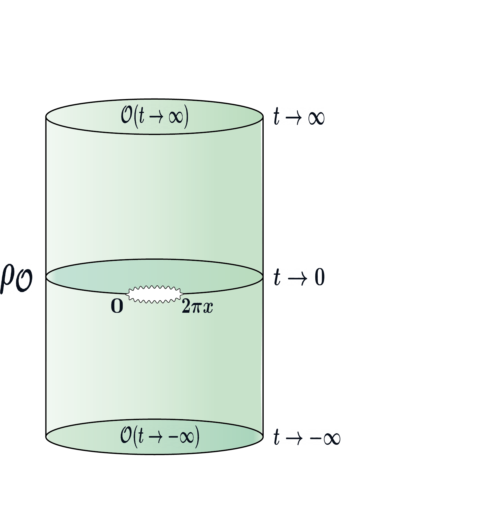
Figure 1: This figure shows the cut cylinder which represents the path integral for the density matrix $\rho_{{\it\mathcal{O}}}$.

The entanglement entropy is obtained by the analytical continuation of the Rényi entropies using the expression

$$\hat{S}_{n}(\rho_{\cal O})=\frac{1}{1-n}\log\big{(}{\rm Tr}\rho_{\cal O}^{n}\big{)},\qquad\hat{S}(\rho)=\lim_{n\rightarrow 1}\hat{S}_{n}(\rho_{\cal O}).$$ (10)

The above formula includes the universal entanglement entropy of the vacuum. It is convenient to subtract this contribution, for this, it is sufficient to evaluate the ratio of traces of the density matrices corresponding of the operator ${\cal O}$ and that of the vacuum.

$$S_{n}(\rho_{\cal O})=\frac{1}{1-n}\log\Big{(}\frac{{\rm Tr}\rho_{\cal O}^{n}}{{\rm Tr}\rho_{(0)}^{n}}\Big{)},\qquad S(\rho)=\lim_{n\rightarrow 1}S_{n}(\rho_{\cal O}).$$ (11)

Here $\rho_{(0)}$ refers to the density matrix without any operator insertions. Using the path integral and conformal transformations the ratio of the traces of the density matrices can be written as the following $2n$-point function on the plane

$$\frac{{\rm Tr}\rho_{\cal O}^{n}}{{\rm Tr}\rho_{(0)}^{n}}=\frac{1}{\big{(}\langle{\cal O}|{\cal O}\rangle\big{)}^{n}}\Big{\langle}\prod_{k=0}^{n-1}w\circ{\cal O}(w_{k})\prod_{k^{\prime}=0}^{n-1}\hat{w}\circ{\cal O}^{*}(\hat{w}_{k})\Big{\rangle}.$$ (12)

Here $w\circ{\cal O}(z)$ refers to the action of the conformal transformation $w(z)$ on the operator ${\cal O}$ where

$$w(z)=\left(\frac{z-u}{z-v}\right)^{\frac{1}{n}},$$ (13)

and

$$u=e^{2\pi ix},\qquad v=1.$$ (14)

This is the map that takes the $n$-branched cylinder to the plane and the operator ${\cal O}$ placed at $t\rightarrow-\infty$ on each cylinder to the following point on the plane.

$$w_{k}=e^{\frac{2\pi i(k+x)}{n}}=\lim_{z\rightarrow 0_{k}}\left(\frac{z-u}{z-v}\right)^{\frac{1}{n}},$$ (15)

where $0_{k}$ refers to the position of the operator ${\cal O}$ on the $k$-th cylinder. Each cylinder is mapped to a wedge on the complex plane. Similarly $\hat{w}\circ{\cal O}(\hat{z})$ refers to the conformal transformation

$$\hat{w}(\hat{z})=\left(\frac{\frac{1}{\hat{z}}-u}{\frac{1}{\hat{z}}-v}\right)^{\frac{1}{n}}.$$ (16)

Thus $\hat{w}(\hat{z})$ is the map that takes the $n$-branched cylinder to the plane and the operator ${\cal O}^{*}$ placed at $t\rightarrow\infty$ on each cylinder to the following point on the plane.

$$\hat{w}_{k}=\lim_{\hat{z}\rightarrow\hat{0}_{k}}\left(\frac{\frac{1}{\hat{z}}-u}{\frac{1}{\hat{z}}-v}\right)^{\frac{1}{n}}=e^{\frac{2\pi ik}{n}}.$$ (17)

Th operator positions in the $2n$-point function in (12) are shown in figure 2.

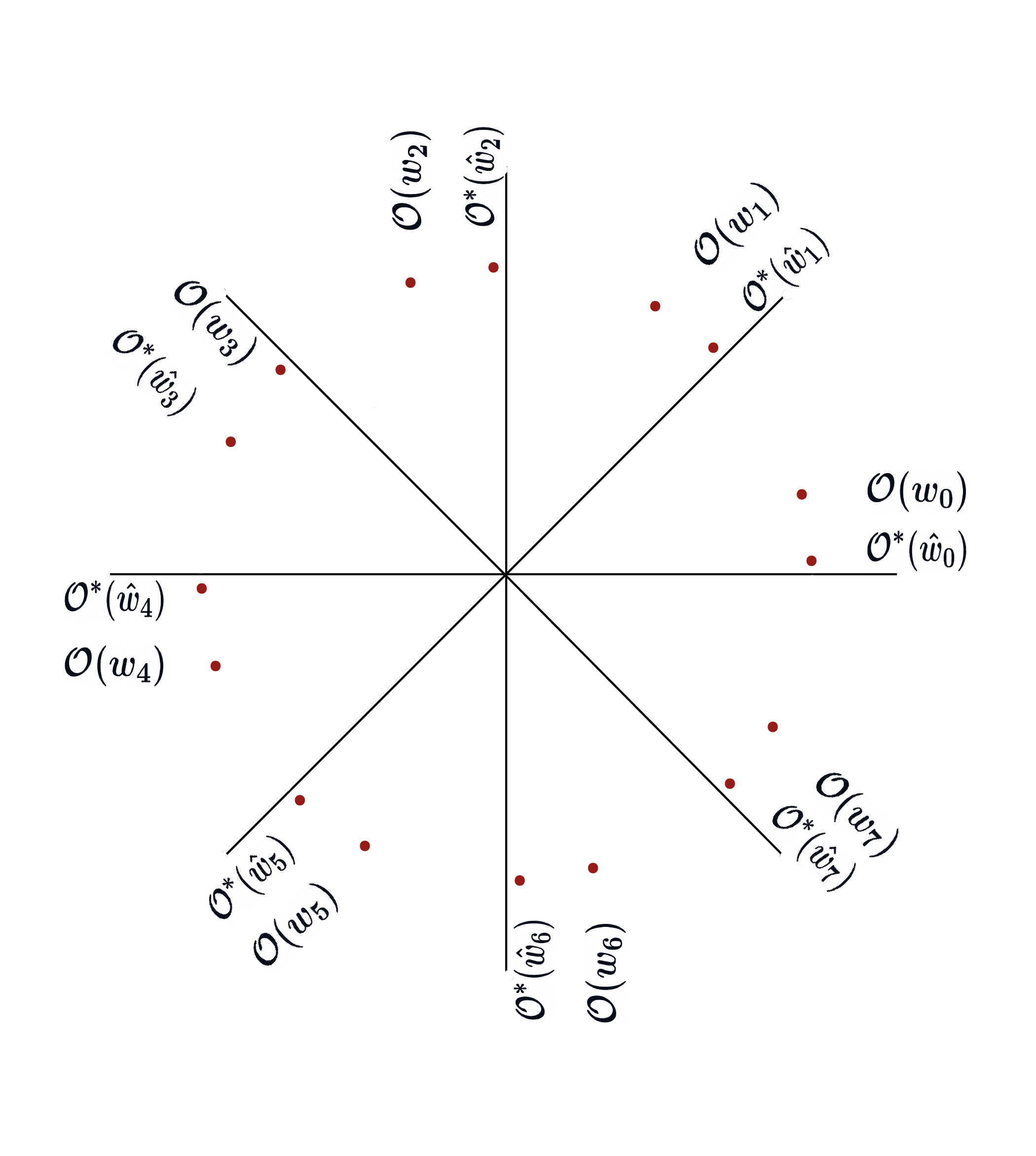
Figure 2: The figure shows the uniformized plane for the $n=8$ replica surface. Each cylinder is mapped to a wedge on the uniformed plane. There are $2n$ operators with a pair of operators on each wedge. The operators are located on the unit circe separated by an arc length of $2\pi x$.

Note that the operators on a given wedge are located on the unit circle and separated by an arc distance of $2\pi x$. The norm $\langle{\cal O}|{\cal O}\rangle$ can be evaluated by using the maps $w(z),\hat{w}(z)$ given in (13), (16) with $n=1$.

2.1 Short distance expansion

In general the $2n$-point function cannot be evaluated exactly but we can resort to the short distance expansion developed in Sarosi:2016oks ; Chowdhury:2021qja . Let us define

$${\cal C}_{(2n)}=\Big{\langle}\prod_{k=0}^{n-1}w\circ{\cal O}(w_{k})\prod_{k^{\prime}=0}^{n-1}\hat{w}\circ{\cal O}^{*}(\hat{w}_{k^{\prime}})\Big{\rangle}.$$ (18)

In the short distance expansion since the distance between the operators ${\cal O}$ and ${\cal O}^{*}$ in a given wedge is small, the leading contribution to the $2n$-point function arises when one factorizes the correlator into $n$ 2-point functions as shown in figure 3.

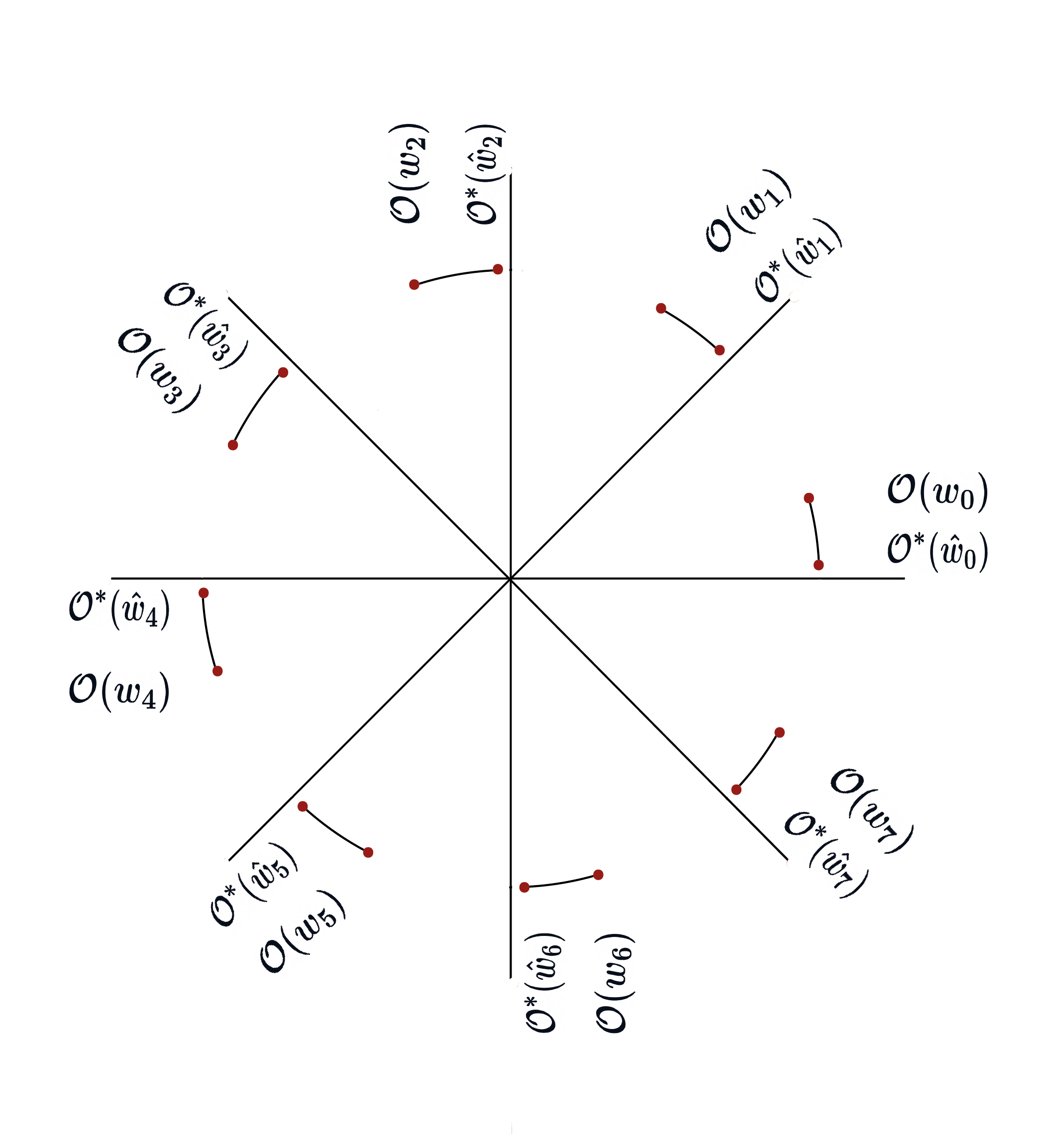
Figure 3: A $n=8$ uniformized plane showing the contraction structure of the $2n$-point function for the leading term in the single interval entanglement entropy. The $2n$-point function is factored into $n$ 2-point function with pairs of operators on the same wedge.

The sub-leading contribution is obtained by factorizing the correlator as demonstrated in the figure 4.

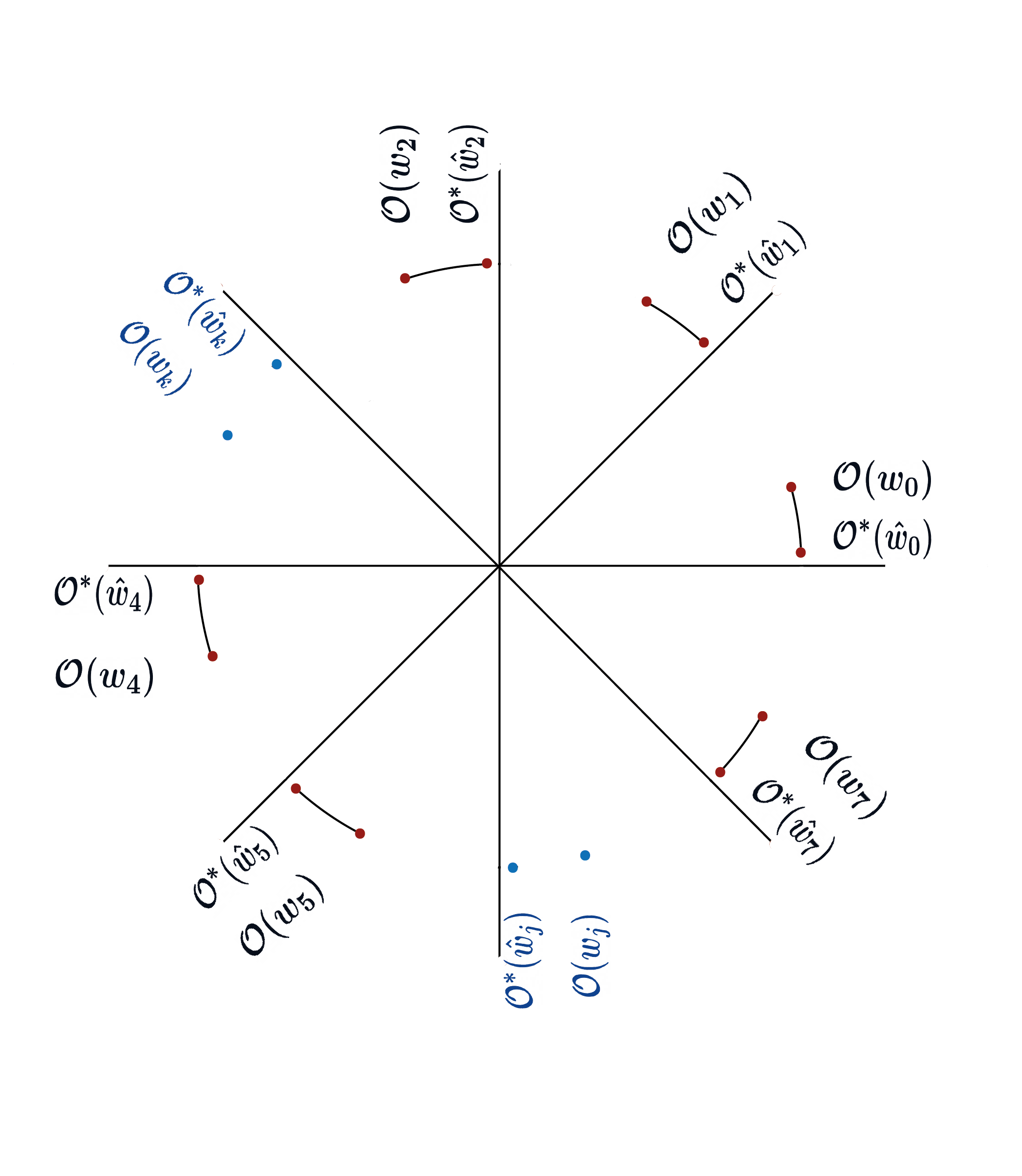
Figure 4: The figure shows a $n=8$ uniformized plane with the factorisation of the $2n$-point function into $(n-2)$, 2-point functions which are contracted on the same wedge and a $4$-point functions involving operators on a pair of wedges which are in blue. The contributions from all such pairs are summed over to obtain the sub-leading contribution to the single interval entanglement entropy.

We write both these contributions as

$${\cal C}_{2n} = {\cal C}_{2n}^{(0)}+{\cal C}_{2n}^{(1)}+\cdots,$$ (19)

$${\cal C}_{2n}^{(0)} = \prod_{k=0}^{n-1}\langle w\circ{\cal O}(w_{k})\hat{w}\circ{\cal O}^{*}(\hat{w}_{k})\rangle,$$ (20)

$${\cal C}_{2n}^{(1)} = \sum_{i,j=0,i\neq j}^{n-1}\left(\prod_{k=0,k\neq i,j}^{n-1}\langle w\circ{\cal O}(w_{k})\hat{w}\circ{\cal O}^{*}(\hat{w}_{k})\rangle\right)\Big{\langle}w\circ{\cal O}(w_{i})w\circ{\cal O}^{*}(\hat{w}_{i})w\circ{\cal O}(w_{j})w\circ{\cal O}^{*}(\hat{w}_{j})\Big{\rangle}_{c}.$$

where the subscript ‘$c$’ refers to the connected correlator. Thus the first sub-leading correction arises from the $4$-point function of the operators on the replica geometry in which a pair of operators are placed on one of the wedges and another pair in another wedge. The rest of the operators are contracted as pairs on the same wedge. The complete contribution involves a sum over all possible pairs of wedges involved in the $4$-point function. Once the $2n$-point function is evaluated we can substitute it in the expression for the entanglement entropy and obtain

$$S(\rho_{\cal O})=\lim_{n\rightarrow 1}\frac{1}{1-n}\log\Big{(}\frac{{\cal C}_{2n}}{(\langle{\cal O}|{\cal O}\rangle)^{n}}\Big{)}.$$ (22)

Leading contribution: 2-point function

In the short distance approximation the leading term (20), is completely determined by the dimension of the operator if it is a primary, if it is a descendant, the result is dependent on the dimension, the level and nature of the descendant and the central charge of the theory. We do not need to know the details of the theory to evaluate the leading term. In this paper we will restrict ourselves to descendants created by the action of the global part of the Virasoro group. If ${\cal O}$ is a primary of weight $(h,0)$ then the two point function on any of the wedges is given by

$$\frac{1}{\langle{\cal O}|{\cal O}\rangle}\big{\langle}w\circ{\cal O}(w_{k})\hat{w}\circ{\cal O}^{*}(\hat{w}_{k})\big{\rangle}=\left(\frac{\sin\pi x}{n\sin\frac{\pi x}{n}}\right)^{2h},\quad k=0,\cdots n-1.$$ (23)

Global descendants of the primary ${\cal O}$ are given by

$$\partial^{l}{\cal O}|0\rangle=(L_{-1})^{l}|h\;0\rangle.$$ (24)

The two point function between descendants of arbitrary levels on a given wedge in the replica geometry is given by

$$\langle w\circ\partial^{l}{\cal O}(w_{k})\hat{w}\circ\partial^{l^{\prime}}{\cal O}(\hat{w}_{k})\rangle = \partial_{z}^{l}\partial_{\hat{z}}^{l^{\prime}}G(z,\hat{z},n)\Big{|}_{(z,\hat{z})=(0_{k},\hat{0}_{k})},$$ (25)

$$G(z,\hat{z},n) = \big{(}\partial_{z}w(z)\partial_{\hat{z}}\hat{w}(\hat{z})\big{)}^{h}\left(\frac{1}{w(z)-\hat{w}(\hat{z})}\right)^{2h}.$$

This expression for the two point function between global descendants can be easily derived from the two point function of the primary and the fact that one needs to take appropriate number of derivatives to obtain the two point function of global descendants. More details of this can be found in Chowdhury:2021qja . Since we are interested in entanglement entropy, it is sufficient to expand the function $G(z,\hat{z},n)$ to the leading order around $n\rightarrow 1$

$$G(z,\hat{z},n)=\frac{1}{(1-z\hat{z})^{2h}}-(n-1)\times\frac{h}{(1-z\hat{z})^{2h}}\left\{2+\log\Big{(}\frac{z-u}{z-v}\Big{)}+\log\Big{(}\frac{1-u\hat{z}}{1-v\hat{z}}\Big{)}\right.$$

$$\qquad\qquad\left.+\frac{2}{(u-v)(1-z\hat{z})}\Big{[}(z-u)(1-v\hat{z})\log\Big{(}\frac{z-u}{z-v}\Big{)}+(v-z)(1-u\hat{z})\log\Big{(}\frac{1-u\hat{z}}{1-v\hat{z}}\Big{)}\Big{]}\right\}$$

$$\qquad\qquad\qquad\qquad\qquad\qquad+O((n-1)^{2}).$$ (26)

For subsequent purpose, it is useful to label the coefficients of the Taylor series expansion of the function $G(z,\hat{z},n)$. Let us define

$$g_{ll^{\prime}}(x,n)=\left.\partial_{z}^{l}\partial_{\hat{z}}^{l^{\prime}}G(z,\hat{z},n)\right|_{(z,\hat{z})=(0_{k},\hat{0}_{k})}.$$ (27)

From the expansion in (2.1), we see that the expansion of these coefficients around $n=1$ is of the form

$$g_{ll^{\prime}}(x,n)=\frac{\Gamma(2h+l)l!}{\Gamma(2h)}\delta_{ll^{\prime}}+(n-1)\hat{g}_{ll^{\prime}}(x)+O((n-1)^{2}),$$ (28)

where

$$\hat{g}_{ll^{\prime}}(x) = \left.\partial_{z}^{l}\partial_{\hat{z}}^{l^{\prime}}\hat{G}(z,\hat{z})\right|_{(z,\hat{z})=(0_{k},\hat{0}_{k})}$$ (29)

$$\hat{G}(z,\hat{z}) = -\frac{h}{(1-z\hat{z})^{2h}}\left\{2+\log\Big{(}\frac{z-u}{z-v}\Big{)}+\log\Big{(}\frac{1-u\hat{z}}{1-v\hat{z}}\Big{)}\right.$$

$$\qquad\qquad\left.+\frac{2}{(u-v)(1-z\hat{z})}\Big{[}(z-u)(1-v\hat{z})\log\Big{(}\frac{z-u}{z-v}\Big{)}+(v-z)(1-u\hat{z})\log\Big{(}\frac{1-u\hat{z}}{1-v\hat{z}}\Big{)}\Big{]}\right\}.$$

We can think of $G(z,\hat{z},n)$ as the generating function from which we can derive the two point function using (25). Note that the norm of the descendant can be read out from (28) from the coefficient of $\delta_{ll^{\prime}}$.

We can now use these results to evaluate the leading contribution to the $2n$-point function for a linear combination of a primary and its descendants

$$|\Psi\rangle=\sum_{l=0}^{\infty}\alpha_{l}(L_{-1})^{l}|h\;0\rangle.$$ (30)

with the norm

$$\langle\Psi|\Psi\rangle=\sum_{l=0}^{\infty}|\alpha_{l}|^{2}\frac{\Gamma(2h+l)l!}{\Gamma(2h)}.$$ (31)

The leading contribution ${\cal C}_{2n}^{(0)}$ is given by

$$\frac{{\cal C}_{2n}^{(0)}}{(\langle\Psi|\Psi\rangle)^{n}}=1+(n-1)\sum_{l,l^{\prime}=0}^{\infty}\frac{\alpha_{l}\alpha_{l^{\prime}}^{*}\hat{g}_{ll^{\prime}}(x)}{\langle\Psi|\Psi\rangle}+O((n-1)^{2}).$$ (32)

Sub-leading term: 4 point function

Let us now examine the 2nd term (2.1) in the short distance expansion of the $2n$ point function ${\cal C}_{2n}$. This term involves the four point function which in general depends on the theory considered. Let us first examine the $4$ point function of conformal primaries places on wedge labelled as $j$ and $k$. Using the conformal block decomposition Perlmutter:2015iya , we can expand the four point function as

$$\langle w\circ{\cal O}(w_{j})\hat{w}\circ{\cal O}^{*}(\hat{w}_{j})w\circ{\cal O}(w_{k})\hat{w}\circ{\cal O}^{*}(\hat{w}_{k})\rangle_{c}=(B_{j}\hat{B}_{j}B_{k}\hat{B}_{k})^{h}\times$$ (33)

$$\frac{1}{(w_{j}-\hat{w}_{j})^{2h}(w_{k}-\hat{w}_{k})^{2h}}\left(\sum_{q=1}^{\infty}\chi_{\rm vac,q}w^{2}{}_{2}F_{1}(q,q,2q,w)+\sum_{p}C_{{\cal O}{\cal O}{\cal O}_{p}}C^{{\cal O}_{p}}_{\;\;{\cal O}{\cal O}}w^{h_{p}}{\cal F}(c,h,h_{p},w)\right).$$

The cross ratio $w$ is defined as

$$w=\frac{(w_{j}-\hat{w}_{j})(w_{k}-\hat{w}_{k})}{(w_{j}-w_{k})(\hat{w}_{j}-\hat{w}_{k})}=\left(\frac{\sin\frac{\pi x}{n}}{\sin\frac{\pi}{n}(j-k)}\right)^{2}.$$ (34)

The first term in the round bracket in (33) is the expansion of the Virasoro block corresponding to the stress tensor exchange in terms of the global $SL(2,C)$ blocks represented by the hypergeometric function ${}_{2}F_{1}(q,q,2q,w)$. The first two coefficients which is sufficient for our purpose are

$$\chi_{1}=0,\qquad\qquad\qquad\chi_{2}=\frac{2h^{2}}{c},$$ (35)

where $c$ is the central charge of the CFT. The second term in the round bracket represent the contribution of the Virasoro blocks of the primaries of dimension $h_{p}$ of the theory. $C_{{\cal O}{\cal O}{\cal O}_{p}}C^{{\cal O}_{P}}_{\;\;{\cal O}{\cal O}}$ is the product of the corresponding structure constants, the Virasoro block admits the following expansion

$${\cal F}(c,h,h_{p};w)=1+O(w).$$ (36)

The $B$’s are derivatives of the conformal transformations to the uniformised plane, they are given by

$$B_{k} = \lim_{z\rightarrow 0_{j}}\partial_{z}w(z)=\frac{1}{n}e^{\frac{2\pi i(x+k)}{n}}(1-e^{-2\pi ix}),$$ (37)

$$\hat{B}_{k} = \lim_{\hat{z}\rightarrow\hat{0}_{j}}\partial_{\hat{z}}\hat{w}(\hat{z})=\frac{1}{n}e^{\frac{2\pi ik}{n}}(1-e^{2\pi ix}).$$

For holographic CFT’s we can be more specific about the $4$-point function. For a generalised free field $h<<c$, therefore the stress tensor block does not contribute at the leading order. The leading operator exchanged is the composite $:{\cal O}^{2}:$ with $h_{p}=2h$ and the product of structure constants $C_{{\cal O}{\cal O}{\cal O}_{p}}C^{{\cal O}_{p}}_{\;\;{\cal O}{\cal O}}=2$ Sarosi:2016oks ; Belin:2018juv ; Chowdhury:2021qja . Therefore in generalised free field theory, the leading contribution to the $4$-point function of primaries of weight $h$ is given by

$$\langle w\circ{\cal O}(w_{j})\hat{w}\circ{\cal O}^{*}(\hat{w}_{j})w\circ{\cal O}(w_{k})\hat{w}\circ{\cal O}^{*}(\hat{w}_{k})\rangle_{c}=(B_{j}\hat{B}_{j}B_{k}\hat{B}_{k})^{h}\times$$ (38)

$$\frac{1}{(w_{j}-\hat{w}_{j})^{2h}(w_{k}-\hat{w}_{k})^{2h}}\left[2\left(\frac{\sin\frac{\pi x}{n}}{\sin\frac{\pi}{n}(j-k)}\right)^{4h}\right]+\cdots.$$

The second class of operators in holographic theories are operators with conformal dimensions $h\sim c$, then the leading contribution to the $4$-point function is given by the stress tensor exchange and determined by $\chi_{2}$

$$\langle w\circ{\cal O}(w_{j})\hat{w}\circ{\cal O}^{*}(\hat{w}_{j})w\circ{\cal O}(w_{k})\hat{w}\circ{\cal O}^{*}(\hat{w}_{k})\rangle_{c}=(B_{j}\hat{B}_{j}B_{k}\hat{B}_{k})^{h}\times$$ (39)

$$\frac{1}{(w_{j}-\hat{w}_{j})^{2h}(w_{k}-\hat{w}_{k})^{2h}}\left[\frac{2h^{2}}{c}\left(\frac{\sin\frac{\pi x}{n}}{\sin\frac{\pi}{n}(j-k)}\right)^{4}\right]+\cdots.$$

From expressions (37) we see that in the leading short distance expansion, we can approximate the prefactors occuring in (38) and (39) using

$$\lim_{x\rightarrow 0}\frac{B_{j}}{w_{j}-\hat{w}_{j}}=\frac{1}{n},\qquad\qquad\lim_{x\rightarrow 0}\frac{\hat{B}_{j}}{w_{j}-\hat{w}_{j}}=-\frac{1}{n}.$$ (40)

Note that once this limit is taken, these factors become independent of $j$, the 2-point functions on the $n-2$ wedges in (33) are also independent of the location of the wedge. This allows to perform the sum over $j,k$ using the following Calabrese:2010he

$$\sum_{j,k,j\neq k}^{n-1}\left(\frac{1}{\sin\frac{\pi}{n}(j-k)}\right)^{2h_{p}} = \sum_{l=1}^{n-1}\frac{n-l}{\big{(}\sin\frac{\pi l}{n}\big{)}^{2h_{p}}},$$

$$= (n-1)\frac{\Gamma(\frac{3}{2})\Gamma(h_{p}+1)}{2\Gamma(h_{p}+\frac{3}{2})}+O((n-1)^{2}).$$

The important point to note is that this sum is proportional to $n-1$ and since we are interested in entanglement entropy, there all the rest of the factors present in the expression for ${\cal C}_{2n}^{(1)}$ can be evaluated in the limit $n\rightarrow 1$. Therefore the $n-2$, 2-point functions present in ${\cal C}_{2n}^{(1)}$ reduce to their norm. Proceeding, we obtain the following result for the sub-leading corrections when ${\cal O}$ is a primary

$$\frac{{\cal C}_{2n}^{(1)}}{\big{(}\langle{\cal O}|{\cal O}\rangle\big{)}^{n}}=(n-1)\frac{\Gamma(\frac{3}{2})\Gamma(2h_{p}+1)}{2\Gamma(2h_{p}+\frac{3}{2})}C_{{\cal O}{\cal O}{\cal O}_{p}}C^{{\cal O}_{p}}_{\;\;{\cal O}{\cal O}}\big{(}\sin\frac{\pi x}{n}\big{)}^{2h_{p}}+O((n-1)^{2}).$$ (42)

Here for generalised free field theory we have

$$C_{{\cal O}{\cal O}{\cal O}_{p}}C^{{\cal O}_{p}}_{\;\;{\cal O}{\cal O}}=2,\qquad\qquad h_{p}=2h,$$ (43)

and for operators of large conformal dimensions, that is $\frac{h}{c}\sim O(1)$ with large $c$, the stress tensor exchange is dominant and we can replace

$$C_{{\cal O}{\cal O}{\cal O}_{p}}C^{{\cal O}_{P}}_{\;\;{\cal O}{\cal O}}\rightarrow\frac{2h^{2}}{c},\qquad\qquad h_{p}=2.$$ (44)

We can now consider the 4-point functions of arbitrary descendants and proceed similarly. In the leading short distance expansion we obtain

$$\lim_{x\rightarrow 0}\langle w\circ\partial^{l}{\cal O}(w_{j})\hat{w}\circ\partial^{l^{\prime}}{\cal O}^{*}(\hat{w}_{j})w\circ\partial^{m}{\cal O}(w_{k})\hat{w}\circ\partial^{m^{\prime}}{\cal O}^{*}(\hat{w}_{k})\rangle_{c}=$$ (45)

$$\frac{(B_{j}^{h+l}\hat{B}_{j}^{h+l^{\prime}}B_{k}^{h+m}\hat{B}_{k}^{h+m^{\prime}})}{(w_{j}-\hat{w}_{j})^{2h+l+l^{\prime}}(w_{k}-\hat{w}_{k})^{2h+m+m^{\prime}}}\times\left(\frac{\sin\frac{\pi x}{n}}{\sin\frac{\pi}{n}(j-k)}\right)^{2h_{p}}D_{ll^{\prime}}(h,h_{p},n)D_{mm^{\prime}}(h,h_{p},n)$$

Thus the four point function changes by a numerical factor $D_{ll^{\prime}}(h,h_{p},n)$, called the dressing factor in Chowdhury:2021qja . The details of this derivation and various examples worked out examples can be found in Chowdhury:2021qja . Again examining the leading short distance limit for the factors $B_{k},\hat{B}_{k}$ given in in (40) we can perform the sum over $j,k$ using (2.1). Thus we need the dressing factor only in the limit $n\rightarrow 1$, which can be obtained by the deformed norm as follows Chowdhury:2021qja . Let us define the maps

$$s(z)=\frac{z}{z-1},\qquad\hat{s}(\hat{z})=\frac{1}{1-\hat{z}},$$ (46)

Then the deformed norm is given by

$$D_{ll^{\prime}}(h,h_{p}) = \lim_{n\rightarrow 1}D_{ll^{\prime}}(h,h_{p},n),$$ (47)

$$D_{ll^{\prime}}(h,h_{p}) = \left.\partial_{z}^{l}\partial_{\hat{z}}^{l^{\prime}}H(z,\hat{z})\right|_{(z,\hat{z})=(0,0)},$$

$$H(z,\hat{z}) = (\partial_{z}s(z)\partial_{\hat{z}}s(\hat{z}))^{h}\left(\frac{1}{s(z)-\hat{s}(\hat{z})}\right)^{2h-h_{p}},$$

$$= \frac{1}{(1-z\hat{z})^{2h-h_{p}}(1-z)^{h_{p}}(1-\hat{z})^{h_{p}}}.$$

Observe that when $h_{p}=0$, the deformed norm reduces to the norm between descendants

$$D_{ll^{\prime}}(h,0)=\frac{\Gamma(2h+l)l!}{\Gamma(2h)}\delta_{ll^{\prime}}.$$ (48)

Using all these inputs, let us evaluate the sub leading contribution (39) to the $2n$-point function corresponding to the state $|\Psi\rangle$ given in (30).

$$\frac{{\cal C}_{2n}^{(1)}}{(\langle\Psi|\Psi\rangle)^{n}} = (n-1)\frac{\Gamma(\frac{3}{2})\Gamma(h_{p}+1)}{2\Gamma(h_{p}+\frac{3}{2})}C_{{\cal O}{\cal O}{\cal O}_{p}}C^{{\cal O}_{p}}_{\;\;{\cal O}{\cal O}}\frac{(\sin\pi x)^{2h_{p}}}{\langle\Psi|\Psi\rangle^{2}}$$

$$\qquad\qquad\times\left(\sum_{l,l^{\prime}=0}^{\infty}\alpha_{l}\alpha_{l^{\prime}}^{*}D_{ll^{\prime}}(h,h_{p})\right)^{2}+O((n-1)^{2}).$$

2.2 Primaries

We can apply the result for the leading and sub-leading contributions to the $2n$-point function and obtain the leading approximations to the short distance expansions of the entanglement entropy. Consider the case of the primary ${\cal O}$ with weight $(h,0)$, let the state be normalised to unity modulo the phase $(-1)^{2h}$ which occurs since we are using the transformation $\hat{I}(z)=\frac{1}{z}$ to define the norm. Then we can evaluate the coefficient which determined the $2$ point functions in (29)

$$\hat{g}_{00}=-2h(1-\pi x\cot\pi x),$$ (50)

and then using (28) we find that

$$g_{00}=1-(n-1)2h(1-\pi x\cot\pi x).$$ (51)

Substituting in the expression for the leading correction to the $2n$ point function, we obtain

$$\frac{{C}_{2n}^{(0)}}{\big{(}\langle{\cal O}|{\cal O}\rangle\big{)}^{n}}=1-(n-1)2h(1-\pi x\cot\pi x)+O((n-1)^{2}).$$ (52)

Let us now proceed to evaluate the sub-leading correction for a generalised free field, then the leading correction is obtained by setting $h_{p}=2h$ and $C_{{\cal O}{\cal O}{\cal O}_{p}}C^{{\cal O}{\cal O}{\cal O}_{p}}=2$. The subleading correction to the $2n$ point function can be read out from (42),

$$\frac{{C}_{2n}^{(1)}}{\big{(}\langle{\cal O}|{\cal O}\rangle\big{)}^{n}}=(n-1)\frac{\Gamma(\frac{3}{2})\Gamma(2h+1)}{\Gamma(2h+\frac{3}{2})}(\sin\pi x)^{4h}+O((n-1)^{2}).$$ (53)

Substituting (52) and (53) into the expression for the entanglement entropy (22), we obtain

$$S\big{(}\rho_{|h,0\rangle}\big{)}=2h(1-\pi x\cot\pi x)-\frac{\Gamma(\frac{3}{2})\Gamma(2h+1)}{\Gamma(2h+\frac{3}{2})}(\pi x)^{4h}+\cdots.$$ (54)

This is the leading short distance expansion of the entanglement entropy for generalised free fields for which the leading contribution to the $4$-point function arises from the composite operator $:{\cal O}^{2}:$.

We now proceed with the case when the operator ${\cal O}$ corresponds to the primary with equal holomorphic and ant-holomorphic weights, so the state we consider is $|h,h\rangle$. Going through the same steps and the fact that 2-point functions factorize into holomorphic and anti-holomorphic parts, we obtain for the leading correction to the $2n$-point function

$$\frac{{C}_{2n}^{(0)}}{\big{(}\langle{\cal O}|{\cal O}\rangle\big{)}^{n}}=1-(n-1)4h(1-\pi x\cot\pi x)+O((n-1)^{2}).$$ (55)

The simplest way to see this is to realize that the 2 point function of these primaries are given by taking $h\rightarrow 2h$ in the equation (23) leading to

$$\frac{1}{\langle{\cal O}|{\cal O}\rangle}\big{\langle}w\circ{\cal O}(w_{k},\bar{w}_{k})\hat{w}\circ{\cal O}^{*}(\hat{w}_{k},\bar{\hat{w}}_{k}))\big{\rangle}=\left(\frac{\sin\pi x}{n\sin\frac{\pi x}{n}}\right)^{4h},\quad k=0,\cdots n-1.$$ (56)

Taking the complex conjugates of the maps in (13), (16) gives the action of the maps on the anti-holomorphic coordinates. Taking $n$ products of the above two point function and then performing the $n\rightarrow 1$ limit results in (55). The sub-leading contribution to the $2n$-point function can be evaluated using the $4$-point function of these primaries in generalized free field theory. This is given by++

$$\langle w\circ{\cal O}(w_{j},\bar{w}_{j})\hat{w}\circ{\cal O}^{*}(\hat{w}_{j},\bar{\hat{w}}_{j})w\circ{\cal O}(w_{k},\bar{w}_{k})\hat{w}\circ{\cal O}^{*}(\hat{w}_{k},\bar{\hat{w}}_{k})\rangle_{c}=|B_{j}\hat{B}_{j}B_{k}\hat{B}_{k}|^{2h}\times$$

$$\frac{1}{|w_{j}-\hat{w}_{j}|^{4h}|w_{k}-\hat{w}_{k}|^{4h}}\left[2\left(\frac{\sin\frac{\pi x}{n}}{\sin\frac{\pi}{n}(j-k)}\right]^{8h}\right]+\cdots.$$ (57)

Using the same steps followed for operators with holomorphic weights, we obtain the following correction to the $2n$ point function

$$\frac{{\cal C}_{2n}^{(1)}}{\big{(}\langle{\cal O}|{\cal O}\rangle\big{)}^{n}}=(n-1)\frac{\Gamma(\frac{3}{2})\Gamma(4h+1)}{\Gamma(4h+\frac{3}{2})}(\sin\pi x)^{8h}+O((n-1)^{2}).$$ (58)

Putting (55) and (58) together, we obtain the following expression for the leading corrections to the single interval entanglement entropy of primaries of weight $(h,h)$.

$$S\big{(}\rho_{|h,h\rangle}\big{)}=4h(1-\pi x\cot\pi x)-\frac{\Gamma(\frac{3}{2})\Gamma(4h+1)}{\Gamma(4h+\frac{3}{2})}(\pi x)^{8h}+\cdots.$$ (59)

2.3 Descendants

Let us first consider the descendants of holomorphic primaries, that is operators of weight $(h,0)$ which are given by

$$|\Psi^{(l)}\rangle=(\partial_{z})^{l}{\cal O}|0\rangle=(L_{-1})^{l}|h,0\rangle.$$ (60)

The norm of this state is given by

$$\langle\Psi^{(l)}|\Psi^{(l)}\rangle=\langle h|L_{1}^{l}L_{-1}^{l}|h\rangle=\frac{\Gamma(2h+l)l!}{\Gamma(2h)}.$$ (61)

The contribution to the $2n$-point function of these descendants can be read out from (32) using the fact that $\alpha_{l}=1$ for the given value of $l$ and zero for the rest.

$$\frac{{\cal C}_{2n}^{(0)}}{\big{[}\langle\Psi^{(l)}|\Psi^{(l)}\rangle\big{]}^{n}}=1-(n-1)\frac{\hat{g}_{ll}(x)}{\langle\Psi^{(l)}|\Psi^{(l)}\rangle}+O((n-1)^{2}),$$ (62)

where $\hat{g}_{ll}$ can be found from (29). Since there are equal number of derivatives with respect to $z$ and $\hat{z}$, we can look at the terms in the function $\hat{G}(z,\hat{z})$ which are functions of the product $z\hat{z}$, these are given by

$$\hat{G}(z,\hat{z})|_{z\hat{z}} = -\frac{h}{(1-z\hat{z})^{2h}}\left\{2+\log\Big{(}\frac{u}{v}\Big{)}\right.$$

$$+\left.\frac{2}{(u-v)(1-z\hat{z})}\Big{[}2z\hat{z}(u-v)-(u+z\hat{z}v)\log\Big{(}\frac{u}{v}\Big{)}\Big{]}\right\}.$$

Then expanding in powers of $z\hat{z}$, we obtain

$$\hat{g}_{ll}(x)=-\frac{\Gamma(2h+l)l!}{\Gamma(2h)}2(h+l)(1-\pi x\cot\pi x).$$ (64)

Using (62) and (64) we obtain

$$\frac{{\cal C}_{2n}^{(0)}}{\big{[}\langle\Psi^{(l)}|\Psi^{(l)}\rangle\big{]}^{n}}=1-(n-1)2(h+l)(1-\pi x\cot\pi x)+O((n-1)^{2}).$$ (65)

The sub-leading term is evaluated using (2.1), for which we need the coefficient $D_{ll}(h,h_{p})$ defined in (47). From its definition we see that

$$D_{ll}(h,2h)=\left(\frac{\Gamma(2h+l)}{\Gamma(2h)}\right)^{2}.$$ (66)

Substituting in (22), we obtain the leading contributions to the entanglement entropy of descendants of a holomorphic primary of weight $(h,0)$

$$S\big{(}\rho_{L_{-1}^{l}|h,0\rangle}\big{)}=2(h+l)(1-\pi x\cot\pi x)-\frac{\Gamma(\frac{3}{2})\Gamma(2h+1)}{\Gamma(2h+\frac{3}{2})}\times\left(\frac{\Gamma(2h+l)}{\Gamma(2h)l!}\right)^{2}(\pi x)^{4h}+\cdots.$$

Let us consider the holomorphic descendants of primaries with weight $(h,h)$. These states are defined by

$$|\hat{\Psi}^{(l,0)}\rangle=\big{(}L_{-1})^{l}|h,h\rangle.$$ (68)

Since the $2$-point function factorises into holomorphic and anti-holomorphic factors, going through the same analysis we obtain the following result for the leading correction to the $2n$-point function on the uniformized plane

$$\frac{{\cal C}_{2n}^{(0)}}{\big{[}\langle\hat{\Psi}^{(l,0)}|\hat{\Psi}^{(l,0)}\rangle\big{]}^{n}}=1-(n-1)2(2h+l)(1-\pi x\cot\pi x).$$ (69)

Again going through the same steps for the sub-leading correction we obtain

$$\frac{{\cal C}_{2n}^{(1)}}{\big{[}\langle\hat{\Psi}^{(l,0)}|\hat{\Psi}^{(l,0)}\rangle\big{]}^{n}}=(n-1)\frac{\Gamma(\frac{3}{2})\Gamma(4h+1)}{\Gamma(4h+\frac{3}{2})}\left(\frac{\Gamma(2h+l)}{\Gamma(2h)l!}\right)^{2}(\pi x)^{8h}+\cdots.$$ (70)

Note that the dressing factor occurs only for the holomorphic sector, while in the remaining terms $h$ is replaced by $h\rightarrow 2h$. Substituting (69) and (70) into the expression for the entanglement entropy we obtain

$$S\big{(}\rho_{L_{-1}^{l}|h,h\rangle}\big{)}=2(2h+l)(1-\pi x\cot\pi x)-\frac{\Gamma(\frac{3}{2})\Gamma(4h+1)}{\Gamma(4h+\frac{3}{2})}\times\left(\frac{\Gamma(2h+l)}{\Gamma(2h)l!}\right)^{2}(\pi x)^{8h}+\cdots.$$

By repeating the analysis for states of form $L_{-1}^{l}\bar{L}_{-1}^{l}|h,h\rangle$, we obtain

$$S\big{(}\rho_{L_{-1}^{l}\bar{L}_{-1}^{l}|h,h\rangle}\big{)}=4(h+l)(1-\pi x\cot\pi x)-\frac{\Gamma(\frac{3}{2})\Gamma(4h+1)}{\Gamma(4h+\frac{3}{2})}\times\left(\frac{\Gamma(2h+l)}{\Gamma(2h)l!}\right)^{4}(\pi x)^{8h}+\cdots.$$

2.4 Linear combinations of descendants

Since entanglement entropy of excited states involves a $2n$ point function, it is certainly does not obey the linear superposition rule when one considers the entanglement of linear combinations of excited states. It is useful to study arbitrary linear combinations of excited states involving primaries and descendants. This is because as we will see subsequently such linear combinations span the complete Hilbert space of single particle states of a minimally coupled scalar in $AdS_{3}$. We will also note that linear combinations of excited states need not to be homogenous in the spatial directions and therefore this offers a means to study entanglement entropy of spatially non-homogenous states.

First let us consider the case of linear combination of holomorphic global descendants of a primary with weight $(h,0)$

$$|\Psi\rangle=\sum_{l=0}^{\infty}c_{l}L_{-1}^{l}|h,0\rangle.$$ (73)

Then the norm of this state is given in (31), using (32) and (2.1) in the expression for entanglement entropy we obtain

$$S(\rho_{|\Psi\rangle}) = \sum_{l,l^{\prime}=0}^{\infty}\frac{c_{l}c_{l^{\prime}}^{*}\hat{g}_{ll^{\prime}}(x)}{\langle\Psi|\Psi\rangle}$$

$$\qquad-\frac{\Gamma(\frac{3}{2})\Gamma(2h+1)}{\Gamma(2h+\frac{3}{2})}\frac{(\pi x)^{4h}}{\langle\Psi|\Psi\rangle^{2}}\times\left(\sum_{l,l^{\prime}=0}^{\infty}c_{l}c_{l^{\prime}}^{*}D_{ll^{\prime}}(h,2h)\right)^{2}+\cdots.$$

Here $\hat{g}_{ll^{\prime}}(x)$ is evaluated using (29). $D_{ll^{\prime}}(h,2h)$ is obtained from its definition in (47), which is given by

$$D_{ll^{\prime}}(h,2h)=\frac{\Gamma(2h+l)\Gamma(2h+l^{\prime})}{\big{(}\Gamma(2h)\big{)}^{2}}.$$ (75)

Again it is important to mention that the result in (2.4) are the leading contributions to the short distance expansion of the single interval entanglement entropy. We can easily generalise the expression for the linear combination of holomorphic global descendants of a primary with weight $(h,h)$.

$$|\hat{\Psi}\rangle=\sum_{l=0}^{\infty}c_{l}L_{-1}^{l}|h,h\rangle.$$ (76)

Going through the same analysis, we obtain

$$S(\rho_{|\hat{\Psi}\rangle}) = \sum_{l,l^{\prime}=0}^{\infty}\frac{c_{l}c_{l^{\prime}}^{*}\hat{g}_{ll^{\prime}}(x)}{\langle\hat{\Psi}|\hat{\Psi}\rangle}+2h(1-\pi x\cot\pi x)$$

$$\qquad-\frac{\Gamma(\frac{3}{2})\Gamma(4h+1)}{\Gamma(4h+\frac{3}{2})}\frac{(\pi x)^{8h}}{\langle\hat{\Psi}|\hat{\Psi}\rangle^{2}}\times\left(\sum_{l,l^{\prime}=0}^{\infty}c_{l}c_{l^{\prime}}^{*}D_{ll^{\prime}}(h,2h)\right)^{2}+\cdots.$$

Again this expression is easy to obtain when one observes that the 2-point function on each wedge factorizes into products of holomorphic and anti-holmorphic parts. This leads to the additional term in the first line of (2.4), then the change of $h\rightarrow 2h$ to some of the terms in the second line is due to the same reason which results in (2.3). As a simple check of (2.4), note that it reduces to (2.3) on choosing $c_{l}=1$ for one particular $l$ and vanishing for the rest.

2.5 Primary and level one descendant

For the purposes of section 3, it is useful to write down the explicit formula of the entanglement entropy of the following linear combination

$$|\Phi\rangle=c_{0}|h\;h\rangle+c_{1}L_{-1}|h\;h\rangle.$$ (78)

The norm of this state is given by

$$\langle\Phi|\Phi\rangle=|c_{0}|^{2}+2h|c_{1}|^{2}.$$ (79)

To evaluate the leading corrections we use (2.4), for which we need the coefficients

$$\hat{g}_{00} = -2h(1-\pi x\cot\pi x),$$ (80)

$$\hat{g}_{01} = h(i+\cot\pi x)(-2\pi x+\sin 2\pi x),$$

$$\hat{g}_{10} = h(-i+\cot\pi x)(-2\pi x+\sin 2\pi x),$$

$$\hat{g}_{11} = -4h(h+1)(1-\pi x\cot\pi x).$$

We have evaluated these coefficients by using (29). Let us write the entanglement entropy as

$$S(\rho_{|\Phi\rangle})=S^{(0)}(\rho_{|\Phi\rangle})+S^{(1)}(\rho_{|\Phi\rangle}),$$ (81)

to represent the leading and subleading contributions. Then using (2.4), the leading short distance contribution to the entanglement entropy of the linear combination in (78) is given by

$$S^{(0)}(\rho_{|\Phi\rangle}) = -\frac{|c_{0}|^{2}\hat{g}_{00}+|c_{1}|^{2}\hat{g}_{11}+c_{0}c_{1}^{*}\hat{g}_{01}+c_{1}c_{0}^{*}\hat{g}_{10}}{|c_{0}|^{2}+2h|c_{1}|^{2}}+2h(1-\pi x\cot\pi x),$$

$$= \frac{1}{|c_{0}|^{2}+2h|c_{1}|^{2}}\times\Bigg{(}\Big{[}4h|c_{0}|^{2}+4h(2h+1)|c_{1}|^{2}\Big{]}(1-\pi x\cot\pi x)$$

$$+h\Big{[}(c_{0}c_{1}^{*}+c_{1}c_{0}^{*})\cot\pi x+i(c_{0}c_{1}^{*}-c_{1}c_{0}^{*})\Big{]}(2\pi x-\sin 2\pi x)\Bigg{)}.$$

Proceeding with the evaluation of the sub-leading correction using the second term in (2.4) we obtain

$$S^{(1)}(\rho_{|\Phi\rangle}) = -\frac{\Gamma(\frac{3}{2})\Gamma(4h+1)}{\Gamma(4h+\frac{3}{2})}\frac{(\sin\pi x)^{8h}}{(c_{0}|^{2}+2h|c_{1}|^{2})^{2}}\times\Big{(}|c_{0}|^{2}+2h(c_{0}c_{1}^{*}+c_{0}^{*}c_{1})+(2h)^{2}|c_{1}|^{2}\Big{)}^{2},$$

One of our goals in section 3 is to reproduce both (2.5) and (2.5) from holography. The expressions shows that leading contribution to the entanglement entropy of the state depends on the spatial coordinate $x$ in a non-trivial way, not just proportional to the function $(1-\pi x\cot\pi x)$ which is the case of the primaries or any of the descendants as in (54), (59), (2.3, (2.3).

Comparison with modular Hamiltonian

It is known that that the leading contributions to the entanglement of the excited state can be obtained by evaluating the expectation value of the modular Hamiltonian arising from the vacuum $K^{(0)}$ in the excited state Belin:2018juv .

$$S^{(0)}(\rho_{|\Phi\rangle})=\frac{\langle\Phi|K^{(0)}|\Phi\rangle}{\langle\Phi|\Phi\rangle}.$$ (84)

where the modular Hamiltonian of an interval in the vacuum on the cylinder is given by

$$K^{0}=\int_{0}^{2\pi x}d\varphi\left(\frac{\cos(\varphi-\frac{\theta}{2})}{\sin\frac{\theta}{2}}-\cot\frac{\theta}{2}\right)\left(T_{yy}(\varphi)+\bar{T}_{\bar{y}\bar{y}}(\varphi)\right).$$ (85)

Here we have taken the length of the cylinder to be $2\pi$ and the length of the interval along the circumference at $t=0$ to be $2\pi x$. A short review detailing the derivation for the above expression for the modular Hamiltonian is provided in the appendix A. $T_{yy}$ and $\bar{T}_{\bar{y}\bar{y}}$ are the holomorphic and anti-holomorphic components of the stress tensor on the cylinder. At the $t=0$ slice on the cylinder they are given by

$$T_{yy}(\varphi)=\sum_{n=-\infty}^{\infty}L_{n}\exp(in\varphi),\qquad\qquad\bar{T}_{\bar{y}\bar{y}}(\varphi)=\sum_{n=-\infty}^{\infty}\bar{L}_{n}\exp(-in\varphi).$$ (86)

Note that evaluating the expectation value of the modular Hamiltonian on the primary $|h,h\rangle$, yields

$$\langle h,h|K^{(0)}|h,h\rangle=4h(1-\pi x\cot\pi x).$$ (87)

which is the entanglement entropy of the excited state. Here it is only the $L_{0}$ and $\bar{L}_{0}$ term in the expansion of the stress tensor in (86) which contributes.

Since the leading contribution to the entanglement entropy of the linear combination in (78) is a non-trivial function it is interesting to see how the entanglement Hamiltonian reproduces the expression (2.5). For this let us evaluate the following expectation values

$$\langle h\;h|K^{(0)}L_{-1}|h\;h\rangle = 2h\int_{0}^{2\pi x}d\varphi\left(\frac{\cos(\varphi-\frac{\theta}{2})}{\sin\frac{\theta}{2}}-\cot\frac{\theta}{2}\right)e^{i\varphi},$$

$$= h(i+\cot\pi x)(2\pi x-\sin 2\pi x).$$

Similarly

$$\langle h\;h|L_{1}K^{(0)}|h\;h\rangle = 2h\int_{0}^{2\pi x}d\varphi\left(\frac{\cos(\varphi-\frac{\theta}{2})}{\sin\frac{\theta}{2}}-\cot\frac{\theta}{2}\right)e^{-i\varphi},$$

$$= h(-i+\cot\pi x)(2\pi x-\sin 2\pi x).$$

Finally we also have

$$\langle h\;h|L_{1}K^{(0)}L_{-1}|h\;h\rangle = (h+1)4h(1-\pi x\cot\pi x)+4h^{2}(1-\pi x\cot\pi x),$$

$$= 4h(2h+1)(1-\pi x\cot\pi x).$$

Here the second term comes from the anti-holomorphic part of the stress tensor in (86). Now using (87), (2.5), (2.5), (2.5) we can evaluate

$$\frac{\langle\Phi|K^{(0)}|\Phi\rangle}{\langle\Phi|\Phi\rangle} = \frac{1}{|a_{0}|^{2}+2h|a_{1}|^{2}}\times\Bigg{(}\Big{[}4h|c_{0}|^{2}+4h(2h+1)|c_{1}|^{2}\Big{]}(1-\pi x\cot\pi x)$$

$$+h\Big{[}(c_{0}c_{1}^{*}+c_{1}c_{0}^{*})\cot\pi x+i(c_{0}c_{1}^{*}-c_{1}c_{0}^{*})\Big{]}(2\pi x-\sin 2\pi x)\Bigg{)}.$$

where the state $|\Phi\rangle$ is given in (78). Observe that the above equation precisely agrees with (2.5), which provides a cross check for the leading contribution to the entanglement entropy evaluated using the replica method.

2.6 Coherent states

In Caputa:2022zsr a class of coherent state was studied both in the CFT and the bulk. These states involve specific linear combinations of the primary and the descendants including Virasoro descendants. The primaries had conformal dimensions $\frac{h}{c}\sim O(1)$ and $c>>1$, therefore it is possible to construct geometries dual to these states. One such state considered by Caputa:2022zsr is the following linear combination

$$|\Psi_{k}(z,\bar{z})\rangle=(1-z_{k}\bar{z}_{k})^{h_{k}}\sum_{l=0}^{\infty}\frac{z_{k}^{l}}{k^{n}l!}L_{-k}^{l}|h\;0\rangle,$$ (92)

where

$$h_{k}=\frac{1}{k}\Big{[}h+\frac{c}{24}(k^{2}-1)\Big{]}.$$ (93)

Based on the expectation value of the stress tensor in this state it was proposed that this coherent state is dual to Ba$\tilde{\rm{n}}$ados geometries Banados:1998gg and an expression for its entanglement entropy for arbitrary $k$ was derived using the Ryu-Takanayagi formula. For the special case of $k=1$, $|\Psi_{1}(z,\bar{z})\rangle$ when the state is a coherent state of global descendants, the Heavy-Heavy-Light-Light correlator was used to demonstrate agreement with the expression for entanglement entropy derived from the Ba$\tilde{\rm{n}}$ados geometry.

Here we will use the general expression for the leading and sub-leading corrections to the entanglement entropy for a linear combination of global descendants to evaluate the single interval entanglement entropy. The state we are interested is $k=1$ of (92), which is given by

$$|\Psi_{1}(z,\bar{z})\rangle=(1-z\bar{z})^{h}\sum_{l=0}^{\infty}\frac{z^{l}}{l!}L_{-1}^{l}|h\;0\rangle$$ (94)

where we have dropped the subscript in $z_{1},\bar{z}_{1}$. Observe that from (61), this state is of unit norm, the coefficients for the linear combination of global descendants are given by

$$c_{l}=(1-z\hat{z})^{h}\frac{z^{l}}{l!},\qquad c_{l}^{*}=(1-z\bar{z})^{h}\frac{\bar{z}^{l}}{l!}$$ (95)

With these coefficients and using the definition (29) we have

$$\sum_{l,l^{\prime}}c_{l}c_{l^{\prime}}^{*}g_{ll^{\prime}}(x,n)=(1+z\bar{z})^{2h}\hat{G}(z,\bar{z})$$ (96)

Therefore from (32) and (22) the leading contribution to the entanglement entropy is given by

$$S^{(0)}(\rho_{|\Psi_{1}\rangle}) = h\left\{2+\log\Big{(}\frac{z-u}{z-v}\Big{)}+\log\Big{(}\frac{1-u\bar{z}}{1-v\bar{z}}\Big{)}\right.$$

$$\qquad\left.+\frac{2}{(u-v)(1-z\bar{z})}\Big{[}(z-u)(1-v\hat{z})\log\Big{(}\frac{z-u}{z-v}\Big{)}+(v-z)(1-u\bar{z})\log\Big{(}\frac{1-u\bar{z}}{1-v\bar{z}}\Big{)}\Big{]}\right\}$$

$$= h\Bigg{\{}2+\frac{\Big{(}2z+2\bar{z}uv-(1+z\bar{z})(u+v)\Big{)}}{(u-v)(1-z\bar{z})}\log\Big{[}\frac{(z-u)(1-v\bar{z})}{(z-v)(1-u\bar{z})}\Big{]}\Bigg{\}}.$$

It is important to note that here $(z,\bar{z})$ are just variables parameterising the coherent state in (94) and $(u,v)$ carry the information of the location of the interval. This result also gives us a physical interpretation for the generating function $\hat{G}(z,\bar{z})$. It is the leading contribution to the entanglement entropy of the coherent state in (94).

We can proceed to evaluate the sub-leading contribution. The state is based on the primary with dimensions $\frac{h}{c}\sim O(1)$. Therefore, the leading contribution will be due to the stress tensor exchange with $h_{p}=2$ and

$$C_{{\cal O}{\cal O}{\cal O}_{p}}C^{{\cal O}_{p}}_{\;{\cal O}{\cal O}}\rightarrow\frac{2h^{2}}{c},$$ (98)

as discussed around (35) and (44) From (2.1) we see that we need the dressing factor, which is given by

$$\sum_{l,l^{\prime}=0}^{\infty}c_{l}c_{l^{\prime}}^{*}D_{ll^{\prime}}(h,2)=\frac{(1-z\bar{z})^{2}}{(1-z)^{h}(1-\bar{z})^{h}},$$ (99)

here we have used the definition (47) and $c_{l}$ from (95). Finally using (2.1) and the definition (22), we obtain the following contribution at the sub-leading level

$$S^{(1)}(\rho_{|\Psi_{1}\rangle}) = -\frac{8h^{2}}{15c}\frac{(1-z\bar{z})^{4}}{(1-z)^{2h}(1-\bar{z})^{2h}}(\pi x)^{4}+\cdots.$$ (100)

In section 3.5, we will show the entanglement entropy evaluated using the Ryu-Takayanagi formula on the Ba$\tilde{\rm{n}}$ados geometry corresponding to the coherent state (94) precisely agree at both with the leading (2.6) and the sub-leading (100) terms in the short distance expansion.

3 Entanglement of single particle states in gravity

In this section we evaluate the single interval entanglement entropy of excited states using the formula proposed by Faulkner-Lewkowycz-Maldacena. Before we proceed we review the proposal. We restrict our attention to excitations which do not change the asymptotic geometry. Consider the interval on the boundary of the asymptotically $AdS_{3}$ geometry labelled as $A$ and its complement $\bar{A}$ in figure 5. The bulk geometry at the $t=0$ slice corresponds to the interior of the circle in the same figure. The FLM proposal states that the result for the entanglement entropy for the interval $A$ is given by the

$$S_{\rho_{A}}=\frac{A(\gamma_{A})}{4G_{N}}+S_{\rm bulk}(\Sigma_{A}).$$ (101)

Here $\gamma_{A}$ is the minimal geodesic in the bulk joining the end points of the interval $A$, and $A(\gamma_{A})$ is its length. $\Sigma_{A}$ is a bulk spatial region contained between $\gamma_{A}$ and the boundary as shown in figure 5. $S_{\rm bulk}(\Sigma_{A})$ is the bulk entanglement entropy evaluated by viewing the bulk as an effective quantum field theory.

Figure 5: The $t=0$ slice of $AdS_{3}$. We consider the entanglement between system $A$ and $\bar{A}$ in the boundary. The minimal surface $\gamma_{A}$ is the geodesic in the bulk connecting the end points of $A$. $\gamma_{A}$ splits the bulk into right(left) wedge denoted by $\Sigma_{A}(\Sigma_{\bar{A}})$. $\gamma_{A}$ consists of: Branch I, where $\varphi^{\prime}(r)<0$ and Branch II with $\varphi^{\prime}(r)>0$. When excitations breaks the isometry in $\varphi$, we need to evaluate the minimal area for the above branches separately.

By the standard rules of AdS/CFT, a primary operator ${\cal O}$ with dimensions $(h,h)$ in the CFT is dual to a minimally coupled scalar $\phi$ propagating in the bulk whose mass is given by

$$M^{2}=\Delta(\Delta-2)=4h(h-1),\qquad\quad\Delta=2h,$$ (102)

here we have assumed the radius of $AdS_{3}$ is unity. In fact all global descendants of the operator ${\cal O}$ are dual to the single particle excitations of the scalar $\phi$. This then allows us to perform a precision check of the FLM formula. We consider various single particle excitations or their linear combinations of the bulk geometry. The bulk geometry is deformed by these excitations and it is necessary to compute the back reacted geometry. The shift in minimal area due to the deformed geometry together with the $S_{\rm bulk}(\Sigma_{A})$ in the FLM formula can be evaluated in the short interval expansion using the methods developed by Belin:2018juv . Combining both the terms in (101) we can evaluate the entanglement entropy of the single particle states and compare it to the results obtained from CFT section 2. This check extends that done in Belin:2018juv for the lowest energy state.

This section is organised as follows, in sub-section 3.1 we review the duality which relates descendants to single particle excitations of the scalar propagating in $AdS$. We focus on $6$ low lying states which are dual to the following descendants in the CFT

$$|\hat{\Psi}^{(1,0)}\rangle=L_{-1}|h\;h\rangle, |\hat{\Psi}^{(2,0)}\rangle=L_{-1}^{2}|h\;h\rangle,$$ (103)

$$|\hat{\Psi}^{(1,1)}\rangle=L_{-1}\bar{L}_{-1}|h\;h\rangle, |\hat{\Psi}^{(2,2)}\rangle=L_{-2}\bar{L}_{-2}|h\;h\rangle,$$

$$|\Phi\rangle=c_{0}|h\;h\rangle+c_{1}L_{-1}|h\;h\rangle, |\Upsilon\rangle=c_{0}|h\;h\rangle+c_{1}L_{-1}\bar{L}_{-1}|h\;h\rangle.$$

In section 3.2, we obtain the back reacted geometry for these states, then in section 3.3, we obtain the shift in minimal area and finally in section 3.4, we evaluate the bulk entanglement entropy. This requires the knowledge of the reduced density matrix of the excited states in the bulk which is obtained using the Bogoliubov transformations which decompose the creation operators of these states into operators interior and exterior of the entangling region $\Sigma_{A}$.

3.1 Construction of single particle states

In this section we construct the single particle states in the bulk which are dual to the conformal primary of dimensions $(h,h)$ and its global descendants. The AdS/CFT dictionary instructs us to examine the minimally coupled scalar of mass (102). The action of this scalar along with that of the metric is given by

$$S=\int d^{3}x\sqrt{-g}\left(\frac{1}{16\pi G_{N}}\left(R+2\right)-\frac{1}{2}\left(\nabla\phi\right)^{2}-\frac{1}{2}M^{2}\phi^{2}\right).$$ (104)

We start with the global $AdS$ solution, which corresponds to the vacuum of the CFT

$$ds^{2}=-(r^{2}+1)dt^{2}+\frac{dr^{2}}{r^{2}+1}+r^{2}d\varphi^{2}\qquad\varphi\sim\varphi+2\pi.$$ (105)

The equations of motion of the scalar in this background is given by

$$(\nabla^{2}-M^{2})\phi(x)=0\,.$$ (106)

We expand the solutions in terms of modes

$$\phi(t,r,\varphi)=\sum_{m,n}\left(a_{m,n}e^{-i\Omega_{m,n}t}e^{im\varphi}f_{m,n}(r)+a^{\dagger}_{m,n}e^{i\Omega_{m,n}t}e^{-im\phi}f^{*}_{m,n}(r)\right)\,.$$ (107)

Here the sum over $m$ runs over the set of integers due to the periodic boundary conditions on $\varphi$. $n$ labels the radial wave function. The solutions which are regular at $r=0$ are given by

$$f_{m,n}(r) = C_{m,n}r^{m}(1+r^{2})^{\frac{\Omega_{m,n}}{2}}{}_{2}F_{1}\Big{(}\frac{1}{2}(m-2h+2+\Omega_{m,n}),\frac{1}{2}(m+2h+\Omega_{m,n}),1+m;-r^{2}\Big{)},$$

$${\rm for}\;\;m>0,$$

$$f_{m,n}(r) = C_{m,n}r^{-m}(1+r^{2})^{\frac{\Omega_{m,n}}{2}}{}_{2}F_{1}\Big{(}\frac{1}{2}(-m-2h+2+\Omega_{m,n}),\frac{1}{2}(-m+2h+\Omega_{m,n}),1-m;-r^{2}\Big{)},$$

$${\rm for}\;\;m<0.$$

Demanding that these functions are normalizable, or bounded at $r\rightarrow\infty$ results in the quantization condition

$$\Omega_{m,n}=2h+|m|+2n,\qquad n=0,1,2,\cdots,{\rm with}\;m\in\mathbb{Z}.$$ (109)

The constants $C_{m,n}$ are fixed using the standard Klein-Gordan inner product which is given by

$$2\Omega_{m,n}\int drd\varphi\sqrt{-g}g^{tt}(r)f_{m,n}(r,\varphi)f_{m^{\prime},n^{\prime}}^{*}(r,\varphi)=\delta_{n,n^{\prime}}\delta_{m,m^{\prime}}\,.$$ (110)

The explicit forms of the wave functions for some low lying states are given in table 1

$m$	$n$	$f_{m,n}(r)$	$L_{0}+\bar{L}_{0}$	$L_{0}-\bar{L}_{0}$
$0$	$0$	$\frac{1}{\sqrt{2\pi}\left(r^{2}+1\right)^{h}}$	$2h$	0
$0$	$1$	$\frac{1}{\sqrt{2\pi}}\frac{2hr^{2}-1}{\left(r^{2}+1\right)^{h+1}}$	$2h+2$	$0$
$0$	$2$	$\frac{1}{\sqrt{2\pi}}\frac{h(2h+1)r^{4}-2(2h+1)r^{2}+1}{\left(r^{2}+1\right)^{h+2}}$	$2h+4$	$0$
$1$	$0$	$\frac{\sqrt{h}r}{\sqrt{\pi}\left(r^{2}+1\right)^{h+\frac{1}{2}}}$	$2h+1$	$1$
$2$	$0$	$\frac{\sqrt{h(2h+1)}r^{2}}{\sqrt{2\pi}\left(r^{2}+1\right)^{h+1}}$	$2h+2$	$2$

Table 1: This table lists the explicit wave functions of the single particle states for low values of $m$ and $n$. The last 2 columns list out the quantum numbers of $L_{0},\bar{L}_{0}$ of the corresponding dual state in the CFT.

From the canonical commutation relations of $\phi$ and $\dot{\phi}$ we obtain that the commutation relations

$$[a_{m,n},a^{\dagger}_{m,n}]=\delta_{n,n^{\prime}}\delta_{m,m^{\prime}}$$ (111)

Therefore single particle states on the global $AdS_{3}$ vacuum are given by

$$|\psi_{m,n}\rangle=a_{m,n}^{\dagger}|0\rangle.$$ (112)

It is clear from the construction, that $m$ and $\Omega_{m,n}$ are the eigen values of the operators corresponding to translations in $\varphi$ and the global time $t$ respectively. Let us use these quantum numbers to relate these states to the global descendants of a primary in the dual CFT. Consider the descendant

$$|\hat{\Psi}^{(n_{1},n_{2})}\rangle=\big{(}L_{-1})^{n_{1}}\big{(}\bar{L}_{-1}\big{)}^{n_{2}}|h\;h\rangle.$$ (113)

Then from the global $SL(2,\mathbb{R})$ algebra we have the following properties for these states

$$(L_{0}+\bar{L}_{0})|\hat{\Psi}^{(n_{1},n_{2})}\rangle = (2h+n_{1}+n_{2})|\hat{\Psi}^{(n_{1},n_{2})}\rangle,$$ (114)

$$(L_{0}-\bar{L}_{0})|\hat{\Psi}^{(n_{1},n_{2})}\rangle = (n_{1}-n_{2})|\hat{\Psi}^{(n_{1},n_{2})}\rangle.$$

From the matching of symmetries we know that the operator $L_{0}-\bar{L}_{0}$ corresponds to the generator of translations along the angular direction $\varphi$ in the bulk. The identification of the global time in $AdS_{3}$ with the time of the CFT, we see that $L_{0}+\bar{L}_{0}$ corresponds to the generator of translations along the global time $t$ in the bulk. This implies that we have the relations

$$2h+n_{1}+n_{2} = \Omega_{m,n}=2h+|m|+2n,$$ (115)

$$n_{1}-n_{2} = m,$$

which gives

$$n_{1}=\frac{|m|+m}{2}+n,\qquad n_{2}=\frac{|m|-m}{2}+n$$ (116)

These relations allow us to identify the single particle excitations in the bulk given in (112) with the global descendants (113) of the primary. The last 2 columns in table 1 are obtained using (116). To summarize, we identify bulk single particle excitations of the minimally coupled scalar with the global descendants of a primary as

$$|\psi_{m,n}\rangle\rightarrow|\hat{\Psi}^{(n_{1},n_{2})}\rangle.$$ (117)

where $(n_{1},n_{2})$ are related to $(m,n)$ using the relations (116).

There is a simple check we can perform to verify the identification in (117). The $SL(2,\mathbb{R})$ generators of the global part of the Virasoro algebra of the CFT can be identified with the isometries of $AdS_{3}$ Maldacena:1998bw . The vector fields corresponding to the left moving $SL(2,\mathbb{R})$ are given by

$$L_{0}=i\partial_{u},$$

$$L_{-1}=ie^{-iu}\left[\frac{\cosh 2\rho}{\sinh 2\rho}\partial_{u}-\frac{1}{\sinh 2\rho}\partial_{v}+\frac{i}{2}\partial_{\rho}\right],$$

$$L_{1}=ie^{iu}\left[\frac{\cosh 2\rho}{\sinh 2\rho}\partial_{u}-\frac{1}{\sinh 2\rho}\partial_{v}-\frac{i}{2}\partial_{\rho}\right].$$ (118)

Here we have used the co-ordinates

$$u=t+\varphi,\qquad v=t-\varphi,\qquad\sinh\rho=r.$$ (119)

The right moving isometries are given by the interchange $u\leftrightarrow v$. Since we have identified the bulk isometries with that of global part of the Virasoro algebra, the states $|\psi_{m,n}\rangle$ must be related to $|\psi_{0,0}\rangle$ by the action of the differential operator $(L_{-1})^{n_{1}}(L_{-1})^{n_{2}}$. Indeed, it is easy to verify that the state $m=1,n=0$ can be obtained by acting $L_{-1}$ on the state $m=0,n=0$

$$L_{-1}\Big{[}f_{0,0}(r)e^{-i2ht}\Big{]}=\sqrt{2h}f_{1,0}(r)e^{-i(2h+1)t-i\varphi}.$$ (120)

Similarly we have the relation

$$L_{-1}^{2}\Big{[}f_{0,0}(r)e^{-i2ht}\Big{]}=\sqrt{(4h)(2h+1)}f_{2,0}e^{-i(2h+2)t-2i\varphi}.$$ (121)

Note that the one particle states in the bulk are of unit norm and the prefactors in (120) and (121) ensure that the normalization agree with that in the CFT.

Now that we have the mapping between single particle states in the bulk to the global descendants of the CFT, we can consider linear combinations of these states and we obtain the dictionary

$$|\Phi\rangle \rightarrow c_{0}|\psi_{0,0}\rangle+\sqrt{2h}c_{1}|\psi_{1,0}\rangle,$$ (122)

$$|\Upsilon\rangle \rightarrow c_{0}|\psi_{0,0}\rangle+2hc_{1}|\psi_{0,1}\rangle.$$

Here the states $|\Phi\rangle$ and $|\Upsilon\rangle$ are states in the CFT defined in (103). The relative factors which depend on $h$ are necessary so that the normalizations agree with that in the CFT. The states $|\psi_{m,n}\rangle$ are unit normalized.

3.2 Backreacted geometry

Once we excite global $AdS_{3}$ by any of the states we discussed in the previous section, the energy density induced by the excited state back reacts when $G_{N}$ is non-vanishing and deforms the geometry. The leading corrections to the entanglement entropy would then be obtained by evaluating the length of minimal surface in the deformed geometry. At the leading oder in $G_{N}$ we can evaluate the back reacted geometry by solving the Einsteins equations with the stress tensor as source. Following the approach in Belin:2018juv , we evaluate the expectation value of the stress tensor of the scalar on the excited states in (103). The stress tensor is given by

$$T_{\mu\nu}=:\partial_{\mu}\phi\partial_{\nu}\phi-\frac{1}{2}g_{\mu\nu}\left((\nabla\phi)^{2}+m^{2}\phi^{2}\right):.$$ (123)

The stress tensor is normal ordered, this ensures that its expectation value on the vacuum vanishes and therefore it implies that we are not sensitive to the UV-divergent zero point energy. These UV effects are state independent and do not affect the calculations. They cancel on considering the entanglement entropy between excited states and the vacuum.

To evaluate the expectation value $\langle\psi|T_{\mu\nu}|\psi\rangle$ we substitute the expansion of $\phi$ given in (107) and use the creation annihilation algebra in (111). This was done for the primary state $|\psi_{0,0}\rangle$ in Belin:2018juv , here we extend this analysis for the states listed in (103). We provide the details for the descendant $|\psi_{0,1}\rangle\rightarrow|\hat{\Psi}^{(1,1)}\rangle$. This state does not have angular momentum so it makes the analysis very similar to that done for the primary in Belin:2018juv . The second state we consider in detail is the linear combination of the primary and the descendant referred to $c_{0}|\psi_{0,0}\rangle+\sqrt{2h}c_{1}|\psi_{1,0}\rangle\rightarrow|\Phi\rangle$. This back reacted geometry corresponding to this state is time dependent and also has angular momentum. The construction of the back reacted geometry is more involved in this case. The analysis for the rest of the states in the list (103) is provided in appendix D.

First excited state with zero angular momentum: $|\psi_{0,1}\rangle$

The non-zero components of the expectation value of the stress tensor on this state are given by

$$\langle\psi_{0,1}|T_{tt}|\psi_{0,1}\rangle=\frac{2h\left(4(2h-1)hr^{2}\left(hr^{2}-1\right)+2h+1\right)+2}{\pi\left(r^{2}+1\right)^{2h+1}},$$ (124)

$$\langle\psi_{0,1}|T_{rr}|\psi_{0,1}\rangle=\frac{2h\left(4hr^{2}\left(hr^{2}-1\right)+3\right)+2}{\pi(1+r^{2})^{2h+3}},$$

$$\langle\psi_{0,1}|T_{\varphi\varphi}|\psi_{0,1}\rangle$$

$$=\frac{2r^{2}\left(h\left(r^{2}\left(4hr^{2}\left(h(1-2h)r^{2}+7h+1\right)-22h-9\right)+3\right)-r^{2}+1\right)}{\pi\left(r^{2}+1\right)^{2h+3}}.$$

As a cross check, we have verified that these components satisfy the conservation law

$$\nabla^{\mu}\langle\psi_{0,1}|T_{\mu\nu}|\psi_{0,1}\rangle=0.$$ (125)

The plot of the expectation value of the energy density of this state, together with the state $|\psi_{0,0}\rangle$ and $|\psi_{0,2}\rangle$ all carrying zero angular momentum is given in figure 6. Note as the level of the descendant increases, the energy density is more de-localized and has increasing number of extrema.

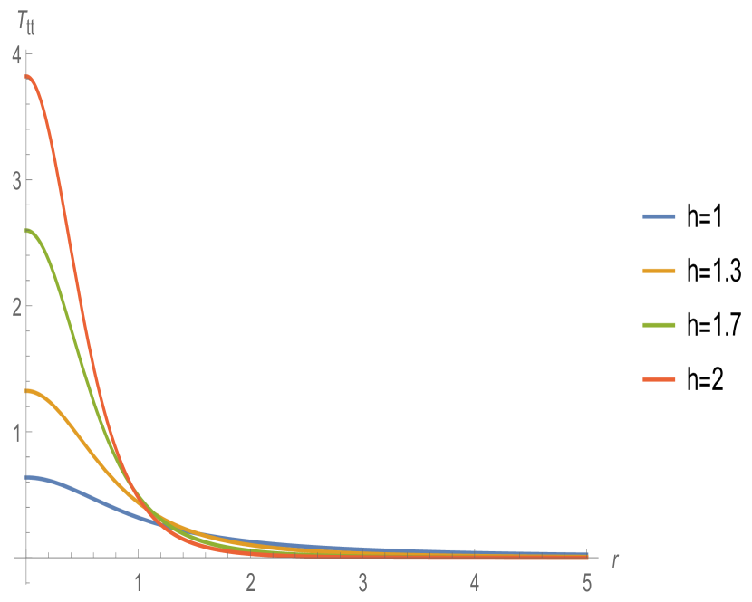
(a)

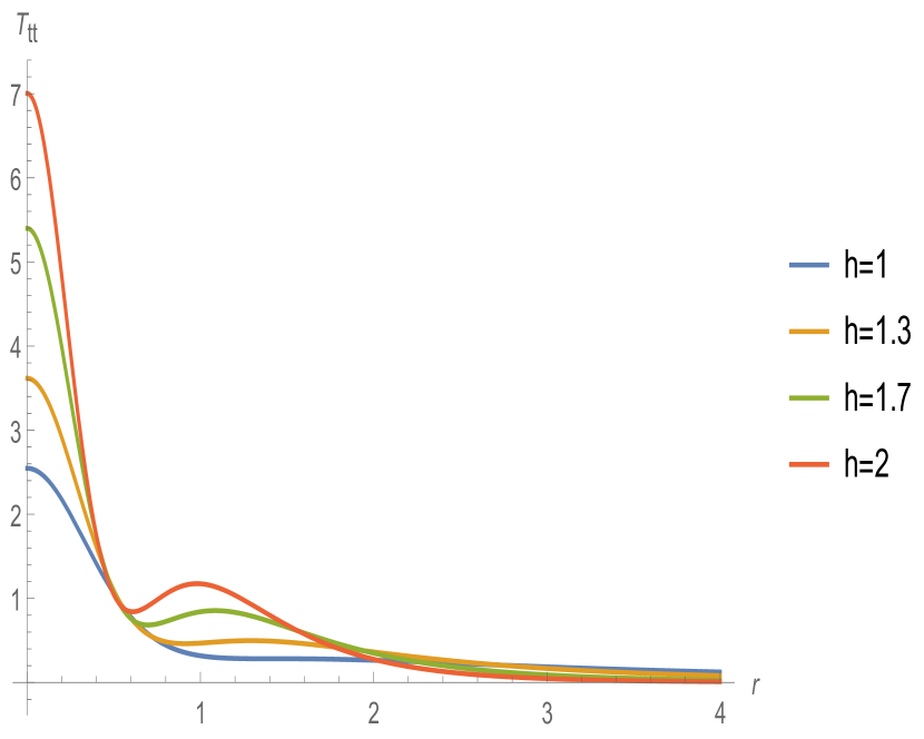
(b)

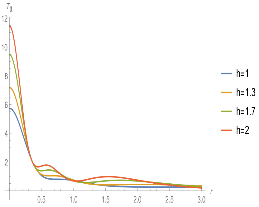
(c)

Figure 6: Expectation value of the energy of the first 3 states with zero angular momentum for a few values of the weight $h$. (a) Energy density in the state $|\psi_{0,0}\rangle$. (b) Energy density in the state $|\psi_{0,1}\rangle$. (c) Energy density in the state $|\psi_{0,1}\rangle$. Note energy density is more de-localized with increasing number of extrema in descendants.

The components of the stress tensor in (124) have only radial dependence and the ones that are non-zero are only the diagonal ones. This is the same property of the expectation value of the stress tensor in the primary $|\psi_{0,0}\rangle$, so we can use the same metric ansatz as in Belin:2018juv which is given by

$$ds^{2} = -(r^{2}+G_{1}(r)^{2})dt^{2}+\frac{dr^{2}}{r^{2}+G_{2}(r)^{2}}+r^{2}d\phi^{2},$$ (126)

$$G_{1}(r) = 1+a(r)G_{N},\qquad\qquad G_{2}(r)=1+b(r)G_{N}.$$

Plugging this ansatz in the Einstein’s equation

$$R_{\mu\nu}-\frac{1}{2}g_{\mu\nu}R-g_{\mu\nu}=8\pi G_{N}\langle\psi|T_{\mu\nu}|\psi\rangle\,,$$ (127)

we obtain the following differential equations for the functions $a(r),b(r)$ at $O(G_{N})$

$$b^{\prime}(r)=-\frac{8r}{(1+r^{2})^{2h+2}}\Big{[}2+2h(1+2h)+8h^{2}(2h-1)r^{2}(hr^{2}-1)\Big{]},$$ (128)

$$(1+r^{2})a^{\prime}(r)-2ra(r)+2rb(r)=\frac{8r}{(1+r^{2})^{2h+1}}\Big{[}2+6h+8h^{2}r^{2}(hr^{2}-1)\Big{]}.$$

These equations result from considering the $tt$ and the $rr$ components of the Einstein’s equation respectively. All the other Einstein’s equations are trivial or trivially satisfied once these equations hold. The solutions for these equations are given by

$$b(r) =A+8\left(4h^{3}r^{4}+2hr^{2}+h+1\right)\left(r^{2}+1\right)^{-2h-1},$$

$$a(r) =\left(16h\frac{r^{2}}{\left(r^{2}+1\right)^{2h+1}}\right)+A+B(1+r^{2}),$$ (129)

where $A$ and $B$ are the constants of integration. It is clear that we need to set $B=0$ so that the metric asymptotes to $AdS_{3}$ at $r\rightarrow\infty$. We can fix the constant $A$ by demanding that the stress tensor evaluated from the bulk using the Fefferman-Graham coordinates agrees with the expectation value of the stress tensor of the CFT in the state $|\hat{\Psi}^{(1,1)}\rangle$. The details of the construction of Fefferman-Graham expansion for the metric in (126) is given in appendix B. From (275), we obtain the following relation

$$\langle\psi_{0,1}|T_{tt}(t,\varphi)|\psi_{0,1}\rangle\Big{|}_{\rm FG}=\frac{1}{4G_{N}}\left(-\frac{1}{2}-G_{N}A\right).$$ (130)

The stress tensor of the CFT on the cylinder is given by

$$T_{tt}(t,\varphi)=\sum_{n=-\infty}^{\infty}(L_{n}e^{in(t+\varphi)}+\bar{L}_{n}e^{in(t-\varphi)})-\frac{c+\bar{c}}{24}.$$ (131)

The expectation value of the CFT stress tensor

$$\frac{\langle\hat{\Psi}^{(1,1)}|T_{tt}(t,\varphi)|\hat{\Psi}^{(1,1)}\rangle}{\langle\hat{\Psi}^{(1,1)}|\hat{\Psi}^{(1,1)}\rangle} = -\frac{c+\bar{c}}{24}+2h+2,$$

$$= -\frac{c}{12}+2h+2,$$

we have used $c=\bar{c}$ to obtain the last line of the above equation. The Brown-Henneaux formula relates the central charge to the Newton’s constant

$$\frac{1}{G_{N}}=\frac{2c}{3}.$$ (133)

Then requiring (130 ) and (3.2) to agree and using (133), we obtain

$$A=-8(h+1).$$ (134)

In Belin:2018juv a similar constant of integration which occurs for the back reacted metric corresponding to the state $\psi_{0,0}\rangle$ was fixed by using the fact that the conical defect of the metric measures the energy of the particle. We find that the above method is more suitable to generalise to the situation when the geometry depends on time and is not isometric in the angular direction. Using (134) and $B=0$, we can write the back reacted metric for the state $|\psi_{0,1}\rangle$ given in (126)

$$G_{1}(r) = 1-8G_{N}(h+1)+\left(16hG_{N}\frac{r^{2}}{\left(r^{2}+1\right)^{2h+1}}\right),$$

$$G_{2}(r) = 1-8G_{N}(h+1)+8G_{N}\frac{\left(4h^{3}r^{4}+2hr^{2}+h+1\right)}{\left(r^{2}+1\right)^{2h+1}}.$$ (135)

Time dependent state with non-zero angular momentum: $c_{0}|\psi_{0,0}\rangle+c_{1}|\psi_{1,0}\rangle$

On evaluating the expectation value of the stress tensor for the state

$$|\hat{\phi}\rangle=c_{0}|\psi_{0,0}\rangle+\sqrt{2h}c_{1}|\psi_{1,0}\rangle,$$ (136)

we note that all the components of the stress tensor are non-vanishing and have angular as well as time dependence. They are given by

$$\frac{\langle\hat{\phi}|T_{tt}|\hat{\phi}\rangle}{\langle\hat{\phi}|\hat{\phi}\rangle}= \frac{1}{|c_{0}|^{2}+2h|c_{1}|^{2}}\frac{1}{\pi}\bigg{\{}2h(2h-1)\left(r^{2}+1\right)^{1-2h}|c_{0}|^{2}+4h^{2}\left(r^{2}+1\right)^{-2h}\left(4h^{2}r^{2}-2hr^{2}+1\right)|c_{1}|^{2}$$

$$+4h^{2}(2h-1)r\left(r^{2}+1\right)^{\frac{1}{2}-2h}\cos(t+\varphi)\left(c_{1}c_{0}^{*}+c_{0}c_{1}^{*}\right)$$

$$-4ih^{2}(2h-1)r\left(r^{2}+1\right)^{\frac{1}{2}-2h}\sin(t+\varphi)\left(c_{1}c_{0}^{*}-c_{0}c_{1}^{*}\right)\bigg{\}},$$

$$\frac{\langle\hat{\phi}|T_{rr}|\hat{\phi}\rangle}{\langle\hat{\phi}|\hat{\phi}\rangle}= \frac{1}{|c_{0}|^{2}+2h|c_{1}|^{2}}\frac{1}{\pi}\bigg{\{}2h\left(r^{2}+1\right)^{-2h-1}|c_{0}|^{2}+8h^{3}r^{2}\left(r^{2}+1\right)^{-2(h+1)}|c_{1}|^{2}$$

$$+4h^{2}r\left(r^{2}+1\right)^{-2h-\frac{3}{2}}\cos(t+\varphi)\left(c_{1}c_{0}^{*}+c_{0}c_{1}^{*}\right)-4ih^{2}r\left(r^{2}+1\right)^{-2h-\frac{3}{2}}\sin(t+\varphi)\left(c_{1}c_{0}^{*}-c_{0}c_{1}^{*}\right)\bigg{\}},$$

$$\frac{\langle\hat{\phi}|T_{\varphi\varphi}|\hat{\phi}\rangle}{\langle\hat{\phi}|\hat{\phi}\rangle}= \frac{1}{|c_{0}|^{2}+2h|c_{1}|^{2}}\frac{1}{\pi}\bigg{\{}-\frac{2hr^{2}\left(r^{2}+1\right)^{-2h-1}\left((2h-1)r^{2}-1\right)}{\pi}|c_{0}|^{2}$$

$$-4h^{2}r^{4}\left(r^{2}+1\right)^{-2(h+1)}\left(4h^{2}r^{2}-2h\left(r^{2}+3\right)-1\right)|c_{1}|^{2}$$

$$-4h^{2}r^{3}\left(r^{2}+1\right)^{-2h-\frac{3}{2}}\left((2h-1)r^{2}-2\right)\cos(t+\varphi)\left(c_{1}c_{0}^{*}+c_{0}c_{1}^{*}\right)$$

$$+4ih^{2}r^{3}\left(r^{2}+1\right)^{-2h-\frac{3}{2}}\left((2h-1)r^{2}-2\right)\sin(t+\varphi)\left(c_{1}c_{0}^{*}-c_{0}c_{1}^{*}\right)\bigg{\}},$$

$$\frac{\langle\hat{\phi}|T_{t\varphi}|\hat{\phi}\rangle}{\langle\hat{\phi}|\hat{\phi}\rangle}= \frac{1}{|c_{0}|^{2}+2h|c_{1}|^{2}}\frac{1}{\pi}\bigg{\{}4h^{2}(2h+1)r^{2}\left(r^{2}+1\right)^{-2h-1}|c_{1}|^{2}+2h^{2}r\left(r^{2}+1\right)^{-2h-\frac{1}{2}}\cos(t+\varphi)\left(c_{1}c_{0}^{*}+c_{0}c_{1}^{*}\right)$$

$$-2ih^{2}r\left(r^{2}+1\right)^{-2h-\frac{1}{2}}\sin(t+\varphi)\left(c_{1}c_{0}^{*}-c_{0}c_{1}^{*}\right)\bigg{\}},$$

$$\frac{\langle\hat{\phi}|T_{rt}|\hat{\phi}\rangle}{\langle\hat{\phi}|\hat{\phi}\rangle}= \frac{1}{|c_{0}|^{2}+2h|c_{1}|^{2}}\frac{1}{\pi}\bigg{\{}2h^{2}r^{2}\left(r^{2}+1\right)^{-2h-\frac{3}{2}}\sin(t+\varphi)\left(c_{1}c_{0}^{*}+c_{0}c_{1}^{*}\right)$$

$$+2ih^{2}r^{2}\left(r^{2}+1\right)^{-2h-\frac{3}{2}}\cos(t+\varphi)\left(c_{1}c_{0}^{*}-c_{0}c_{1}^{*}\right)\bigg{\}},$$

$$\frac{\langle\hat{\phi}|T_{r\varphi}|\hat{\phi}\rangle}{\langle\hat{\phi}|\hat{\phi}\rangle}= \frac{1}{|c_{0}|^{2}+2h|c_{1}|^{2}}\frac{1}{\pi}\bigg{\{}2h^{2}\left(r^{2}+1\right)^{-2h-\frac{1}{2}}\sin(t+\varphi)\left(c_{1}c_{0}^{*}+c_{0}c_{1}^{*}\right)$$

$$+2ih^{2}\left(r^{2}+1\right)^{-2h-\frac{1}{2}}\cos(t+\varphi)\left(c_{1}c_{0}^{*}-c_{0}c_{1}^{*}\right)\bigg{\}}.$$ (137)

Just to recall these are evaluated by substituting the mode expansion (107) into the expression for the stress tensor in (123) and using the algebra of creation and annihilation operators. We have verified that these components satisfy the conservation law. Another simple check is that on setting $c_{1}=0$, observe that stress tensor reduces to that of the primary state evaluated in Belin:2018juv . Also setting $c_{0}=0$, we see that it reduces to the stress tensor evaluated in the appendix for the state $|\psi_{1,0}\rangle$.

It is clear from the expectation values in (3.2), the stress energy is both time dependent as well spatially in-homogenous. It is interesting to plot the expectation value of the energy density as a function of the radial distance for different angles at $t=0$. These plots are given in figure 7.

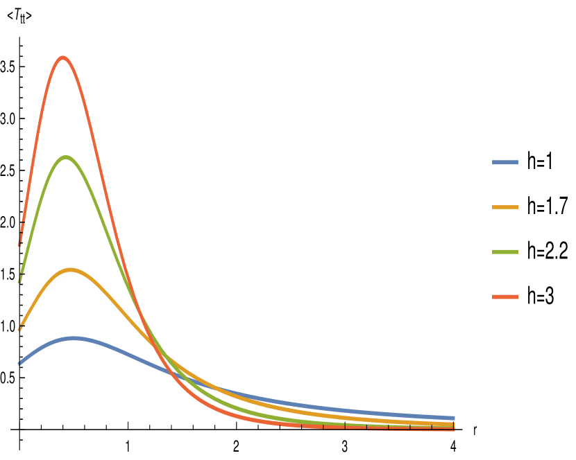
(a)

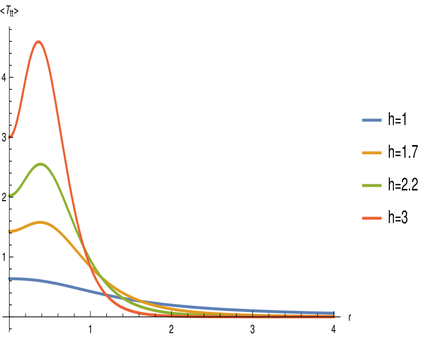
(b)

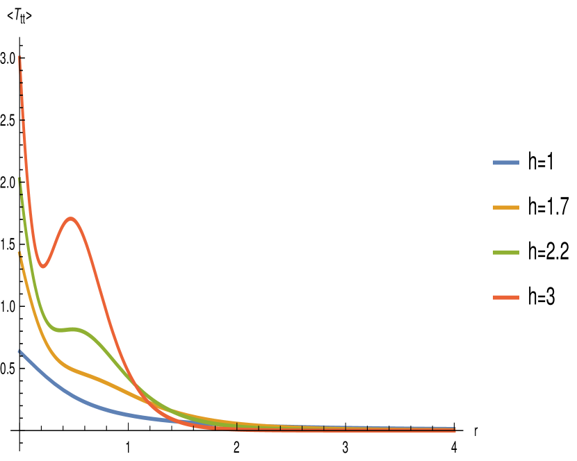
(c)

(d)

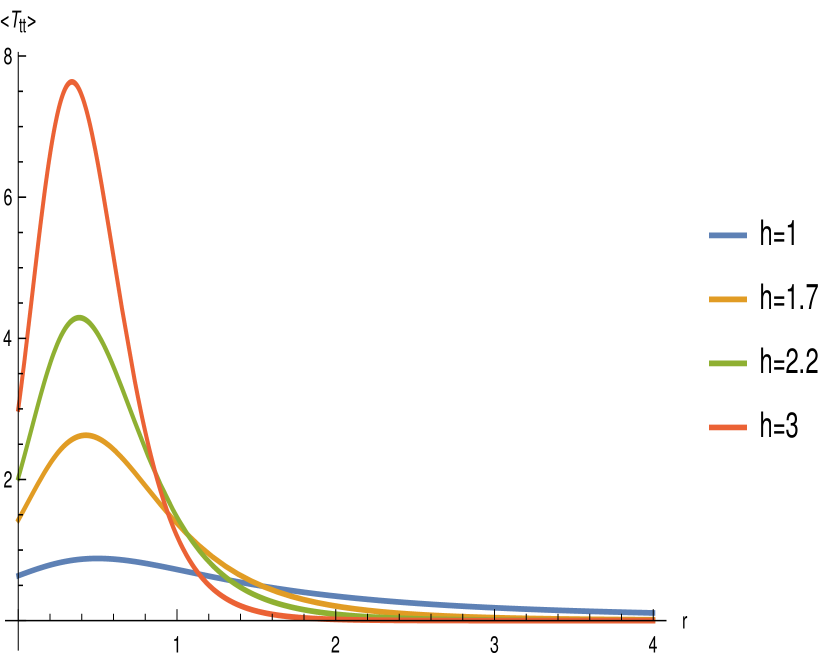
(e)

Figure 7: Expectation value of the energy for the state $|\hat{\phi}\rangle=c_{0}|\psi_{0,0}\rangle+\sqrt{2h}c_{1}|\psi_{1,0}\rangle$ with $c_{0}=c_{1}=1$ and $t=0$. (a) Energy density at $\varphi=0$. (b) Energy density at $\varphi=\frac{\pi}{2}$. (c) Energy density at $\varphi=\pi$.(d) Energy density at $\varphi=\frac{3\pi}{2}$. (e) Energy density at $\varphi=2\pi$.

To solve Einstein’s equation we substitute the stress tensor(3.2) as the source in (127) and take the following ansatz

$$ds^{2} = \Big{[}1+r^{2}+J_{1}(t,r,\varphi)\Big{]}dt^{2}+2J_{2}(t,r,\varphi)drdt+2J_{3}(r)dtd\varphi$$ (138)

$$\qquad\qquad+\frac{dr^{2}}{1+r^{2}+J_{4}(t,r,\varphi)}+r^{2}d\varphi^{2}.$$

Here we have introduced arbitrary functions for the $4$ components. We make a further ansatz for the dependence of these $4$ components which is given below.

$$J_{1}(t,r,\varphi)\text{=}\frac{G_{N}}{(|c_{0}|^{2}+2h|c_{1}|^{2})}\bigg{\{}2|c_{0}|^{2}a_{0,0}(r)+2(2h)|c_{1}|^{2}a_{1,0}(r)\bigg{\}},$$ (139)

$$J_{2}(t,r,\varphi)\text{=}\frac{G_{N}}{(|c_{0}|^{2}+2h|c_{1}|^{2})}\sqrt{2h}\bigg{\{}[R_{2}(r)(c_{1}c_{0}^{*}+c_{0}c_{1}^{*})\sin(t+\varphi)$$

$$\qquad\qquad\qquad+i\tilde{R}_{2}(r)(c_{1}c_{0}^{*}-c_{0}c_{1}^{*})\cos(t+\varphi)\bigg{\}},$$

$$J_{3}(t,r,\varphi)\text{=}\frac{G_{N}}{(|c_{0}|^{2}+2h|c_{1}|^{2})}\bigg{\{}|c_{0}|^{2}b_{0,0}(r)+(2h)|c_{1}|^{2}b_{1,0}(r)$$

$$+\sqrt{2h}[R_{3}(r)(c_{1}c_{0}^{*}+c_{0}c_{1}^{*})\cos(t+\varphi)-i\tilde{R}_{3}(r)(c_{1}c_{0}^{*}-c_{0}c_{1}^{*})\sin(t+\varphi)]\bigg{\}},$$

$$J_{4}(t,r,\varphi)\text{=}\frac{G_{N}}{(|c_{0}|^{2}+2h|c_{1}|^{2})}\bigg{\{}2|c_{0}|^{2}d_{0,0}(r)+2(2h)|c_{1}|^{2}d_{1,0}(r)$$

$$+2\sqrt{2h}[R_{4}(r)(c_{1}c_{0}^{*}+c_{0}c_{1}^{*})\cos(t+\varphi)-i\tilde{R}_{4}(r)(c_{1}c_{0}^{*}-c_{0}c_{1}^{*})\sin(t+\varphi)]\bigg{\}}.$$

One can arrive at this ansatz by requiring that when either $c_{0}$ or $c_{1}$ is set to zero the metric reduces to the back reacted solution for the primary $|\psi_{0,0}\rangle$ or the state $|\psi_{1,1}\rangle$ respectively. Therefore from the results of Belin:2018juv which is also reviewed in appendix D, we get

$$a_{0,0}(r) = -8h,\qquad b_{0,0}(r)=0,\qquad d_{0,0}(r)=-8h+\frac{8h}{\left(r^{2}+1\right)^{2h-1}},$$ (140)

and (346) we get

$$a_{1,0}(r) = 4\left(r^{2}+1\right)^{-2h}-4(2h+1),$$ (141)

$$b_{1,0}(r) = 4\left(r^{2}+1\right)^{-2h},$$

$$d_{1,0}(r) = 4\left(4h^{2}r^{2}+2h+1\right)\left(r^{2}+1\right)^{-2h}-4(2h+1).$$

The rest of the terms in the ansatz are either proportional to ${\rm Re}(c_{0}c_{1}^{*})$ or ${\rm Im}(c_{0}c_{1}^{*})$. From the stress tensor in (3.2), we see that these terms come together with either $\sin(t+\varphi)$ or $\cos(t+\varphi)$. There is a simplifying case of setting $c_{0}=c_{1}=1$ which switches off the terms proportional to ${\rm Im}(c_{0}c_{1}^{*})$. This also helps in arriving at the ansatz in (138), (139).

We substitute the metric in the Einstein equation with the stress tensor given in (3.2) as the source and solve for $R_{2},\tilde{R}_{2},R_{3},\tilde{R}_{3},R_{4},\tilde{R}_{4}$. Though the Einstein’s equations seem to over constrain these functions, there is a consistent solution. The $tt$ component of the Einstein’s equations results in 2 equations, one which arises as the coefficient of ${\rm Re}\;(c_{0}c_{1}^{*})$ which is given by

$$r(r^{2}+1)R_{4}^{\prime}(r)+R_{4}(r)=-\frac{16(2h-1)h\sqrt{2h}\;r^{3}}{(1+r^{2})^{2h-\frac{1}{2}}}\qquad:tt$$ (142)

The equation which arises as the coefficient for ${\rm Im}\;(c_{0}c_{1}^{*})$ results in an identical equation for $\tilde{R}_{4}(r)$,

$$r(r^{2}+1)\tilde{R}_{4}^{\prime}(r)+\tilde{R}_{4}(r)=-\frac{16(2h-1)h\sqrt{2h}\;r^{3}}{(1+r^{2})^{2h-\frac{1}{2}}}\qquad:tt$$ (143)

This feature is seen for all the components of the Einstein equations. That is, the equations which arise as the coefficient of ${\rm Re}\;(c_{0}c_{1}^{*})$ are equations that determine the functions $R_{2},R_{3},R_{4}$, while the equations which arise as the coefficient of ${\rm Im}\;(c_{0}c_{1}^{*})$ determine the functions $\tilde{R}_{2},\tilde{R}_{3},\tilde{R}_{4}$ are identical. Therefore we write the remaining equations that result from the Einstein equations just from the ${\rm Re}\;(c_{0}c_{1}^{*})$.

$$r(1+r^{2})R_{2}(r)+2r^{2}R_{4}(r)-R_{3}(r)=\frac{16h\sqrt{2h}\;r^{3}}{(1+r^{2})^{2h-\frac{1}{2}}},\qquad\qquad\qquad\qquad\qquad\qquad\qquad\qquad\qquad:rr$$

$$(1+r^{2})^{2}R_{2}^{\prime}(r)+r(1+r^{2})R_{2}(r)+(1+r^{2})\Big{[}rR_{4}^{\prime}(r)+R_{4}(r)\Big{]}=-\frac{16h\sqrt{2h}\;r[(2h-1)r^{2}-1]}{(1+r^{2})^{2h-\frac{1}{2}}},\quad:\varphi\varphi$$

$$(1+r^{2})^{2}(rR_{2}^{\prime}(r)-rR_{3}^{\prime\prime}(r)+R_{3}^{\prime}(r))+(1-r^{4})R_{2}(r)-2rR_{4}(r)=\frac{16h\sqrt{2h}\;r^{2}}{(1+r^{2})^{2h-\frac{1}{2}}},\qquad\qquad\quad\quad:t\varphi$$

$$r(1+r^{2})R_{3}^{\prime}(r)-2(1+r^{2})R_{3}(r)+r(1+r^{2})R_{2}(r)+2r^{2}R_{4}(r)=\frac{16h\sqrt{2h}\;r^{3}}{(1+r^{2})^{2h-\frac{1}{2}}},\qquad\qquad\quad\quad:r\varphi$$

$$-(1+r^{2})R_{3}^{\prime}(r)+2r(R_{3}(r)+R_{4}(r))+(1+r^{2})R_{2}(r)=\frac{16h\sqrt{2h}\;r^{2}}{(1+r^{2})^{2h-\frac{1}{2}}}\qquad\qquad\qquad\qquad\qquad:rt$$

To emphasize again, the equations for $\tilde{R}_{2},\tilde{R}_{3}$ and $\tilde{R}_{4}$ are identical to the above equations with the $R_{2}\rightarrow\tilde{R}_{2},R_{3}\rightarrow\tilde{R}_{3}$ and $R_{4}\rightarrow\tilde{R}_{4}$. The solutions to these equations are given by

$$R_{4}(r) = \frac{A\sqrt{r^{2}+1}}{r}+\frac{4\sqrt{2h}\left(2hr^{2}+1\right)}{r\left(r^{2}+1\right)^{2h-\frac{1}{2}}},$$

$$R_{2}(r) = \frac{B}{\sqrt{r^{2}+1}}-\frac{8\sqrt{2h}}{\left(r^{2}+1\right)^{2h+\frac{1}{2}}},$$

$$R_{3}(r) = (2A+B)r\sqrt{1+r^{2}},$$ (145)

and

$$\tilde{R}_{4}(r) = \frac{\tilde{A}\sqrt{r^{2}+1}}{r}+\frac{4\sqrt{2h}\left(2hr^{2}+1\right)}{r\left(r^{2}+1\right)^{2h-\frac{1}{2}}},$$

$$\tilde{R}_{2}(r) = \frac{\tilde{B}}{\sqrt{r^{2}+1}}-\frac{8\sqrt{2h}}{\left(r^{2}+1\right)^{2h+\frac{1}{2}}},$$

$$\tilde{R}_{3}(r) = (2\tilde{A}+\tilde{B})r\sqrt{1+r^{2}}.$$ (146)

Observe that the solutions $R$ and $\tilde{R}$ just differ in the constants of integration. Further more demanding that the metric in (138) asymptotes to $AdS_{3}$ at $r\rightarrow\infty$, we must have

$$2A+B=0,\qquad\qquad 2\tilde{A}+\tilde{B}=0.$$ (147)

We just need to fix two constants $A$ and $\tilde{A}$. For this we can appeal to the same method followed in the case of the state $|\psi_{0,1}\rangle$. From the construction of the Fefferman-Graham expansion of the metric in (138) given in the appendix B we see that the expectation value of the boundary stress tensor in the state (136) is given by (B)

$$\langle\hat{\phi}|T^{FG}_{tt}(t,\varphi)|\hat{\phi}\rangle=\frac{1}{4G_{N}}\left[-\frac{1}{2}+\frac{4G_{N}\Big{[}2h|c_{0}|^{2}+2h(2h+1)|c_{1}|^{2}\Big{]}}{|c_{0}|^{2}+2h|c_{1}|^{2}}\right.$$ (148)

$$\left.-\frac{AG_{N}\sqrt{2h}\Big{[}\big{(}c_{0}c_{1}^{*}+c_{1}c_{0}^{*}\big{)}\cos(t+\varphi)+i\big{(}c_{0}^{*}c_{1}-c_{1}^{*}c_{0}\big{)}\sin(t+\varphi)\Big{]}}{|c_{0}|^{2}+2h|c_{1}|^{2}}\right].$$

The expectation value of the stress tensor of the corresponding dual state $|\Phi\rangle$ in the CFT using (131) is given by

$$\frac{\langle\Phi|T_{tt}(t,\varphi)|\Phi\rangle}{\langle\Phi|\Phi\rangle} = -\frac{c}{12}+\frac{2h|c_{0}|^{2}+2h(2h+1)|c_{1}|^{2}}{|c_{0}|^{2}+2h|c_{1}|^{2}}$$

$$+\frac{2h}{|c_{0}|^{2}+2h|c_{1}|^{2}}\Big{[}(c_{0}^{*}c_{1}+c_{0}c_{1}^{*})\cos(t+\varphi)+i(c_{0}^{*}c_{1}-c_{1}^{*}c_{0})\sin(t+\varphi)\Big{]}.$$

Then comparing (148) and (3.2) to agree we find that

$$A=-\tilde{A}=-4\sqrt{2h},$$ (150)

and then using (147) we get

$$B=-\tilde{B}=8\sqrt{2h}.$$ (151)

To summarize, the back reacted geometry corresponding to the state (136) is given by the metric (138) with the functions (139) along with (140), (141) and with (145) and (146).

The back reacted geometry for the rest of the states in the list (103) are constructed in the appendix D using the same methods.

3.3 Perturbed minimal area

Now that the back reacted geometry is constructed we can use it to evaluate the entanglement entropy from the bulk using the Ryu-Takayanagi formula. This is the first term in the FLM formula in (101), the length of the minimal geodesic between the two end points of the interval on the boundary CFT. This is shown as the curve $\gamma_{A}$ in figure 5. The curve connects these ends points at the time $t=0$. Since we are interested in the difference in entanglement entropy between the ground state and the single particle excited state, it is sufficient to consider the correction to the minimal length. We have found the back reacted metric to the leading order in $G_{N}$, therefore to the leading order the change in minimal area is given by

$$\delta A=A[g_{0}+\delta g]-A[g_{0}]$$ (152)

Where $A[g]$ refers to the length of the geodesic $\gamma_{A}$ evaluated with the metric $g$ and $g_{0}$ is the metric of global $AdS_{3}$ and $g_{0}+\delta g$ is the back reacted metric.

The minimal length in the global $AdS_{3}$ metric $g_{0}$, is given by minimizing the functional

$$A[g_{0}]=2\int_{r_{\min}}^{\infty}dr\sqrt{\frac{1}{r^{2}+1}+r^{2}(\varphi^{\prime}(r))^{2}}\,,$$ (153)

where $r_{m}$ is the turning point on the geodesic. The geodesic is determined by the differential equation

$$\varphi^{\prime}(r)=-\frac{r_{m}}{r\sqrt{\left(r^{2}+1\right)\left(r^{2}-r_{m}^{2}\right)}}\qquad:{\rm Branch\;I},$$ (154)

$$\varphi^{\prime}(r)=\frac{r_{m}}{r\sqrt{\left(r^{2}+1\right)\left(r^{2}-r_{m}^{2}\right)}}\qquad:{\rm Branch\;II}$$

The two signs for the slopes are allowed due to the fact that there is a turning point ar $r_{m}$. In Branch I, the angle increases as $r$ decreases towards $r_{m}$ from infinity and in Branch II, the angle continues to increase as $r$ increases from $r_{m}$ to infinty. The integration constants in Branch I part of the geodesic is fixed by demanding that the angle $\varphi$ is the initial location of the geodesic say $\varphi=0$ at $r\rightarrow\infty$. In Branch II, the integration constant is fixed by demanding that the angle agrees with that of Branch I at the turning point, so that the geodesic is continuous at $r=r_{m}$. We will choose the initial angle $\varphi=0$ since this is one of the end points of interval we have chosen as we see from (14). This results in the following equation for $\varphi$

$$\varphi = \frac{\pi}{2}-\arctan\left(\frac{r^{2}+\sqrt{(1+r^{2})(r^{2}-r_{m}^{2})}}{r_{m}}\right),\qquad{\rm Branch\;I}$$

$$= \frac{\pi}{2}-\arctan\left(\frac{r^{2}-\sqrt{(1+r^{2})(r^{2}-r_{m}^{2})}}{r_{m}}\right),\qquad{\rm Branch\;II}.$$

Let us define

$$\pi x=\arctan\frac{1}{r_{m}}={\rm arccot}\;r_{m}\equiv\frac{\theta}{2}.$$ (156)

In Branch I, the angle $\varphi$ increases from $0$ to $\pi x$ as $r$ takes values from $\infty$ to $r_{m}$ and in Branch II, the angle $\varphi$ increases from $\pi x$ to $2\pi x$. Therefore the total size of the interval is $2\pi x=\theta$. We need to be careful about obtaining the curves precisely and locating the end points of the geodesic at $\varphi=0$ and $\varphi=\theta$ because we will need to deal with the situation when the perturbed metric breaks the isometry in the $\varphi$ direction and therefore the answer will dependent on the location of the end points and not just the opening angle. We have chosen the end points of the geodesic so as to agree with the choice we made in (14) for the end points of the interval in the CFT.

Since we are interested in the correction to the leading order in $G_{N}$ as given in (152), it is easy to see that the geodesic is unchanged at this order since it is the minimal curve and change in the area at order $G_{N}$ is obtained by substituting the shifted metric and integrating it along the geodesic. Let the coefficient of $g_{rr}$ be given as in (3.3)

$$g_{rr}=\frac{1}{1+r^{2}+J_{4}(t,r,\varphi)}.$$ (157)

This form of this metric coefficient is general and it also takes care of the situation when the change in metric is independent of the angle or time. Note that the the coefficient $g_{\varphi\varphi}$ and $g_{r\varphi}$ remains unaltered in the back reacted metrics (126), (138). Therefore the shift in the minimal area is given by

$$\delta A=-\frac{1}{2}\int_{\gamma_{A}}drJ_{4}(t=0,r,\varphi)\frac{(r^{2}-r_{\rm min}^{2})^{\frac{1}{2}}}{r(1+r^{2})^{\frac{3}{2}}},$$ (158)

where the integral is taken along the geodesic curve given in (3.3). We set $t=0$ since we have chosen this time slice to evaluate the entanglement entropy.

Area shift for the state $|\psi_{0,1}\rangle$

Let us now apply this to the back reacted geometry corresponding to the states $|\psi_{0,1}\rangle$. Reading out the perturbed metric from (126) with (3.2), (134) and applying in the expression (158), we are led to evaluate the integral

$$\delta A_{|\psi_{0,1}\rangle}=2G_{N}\int_{r_{\rm min}}^{\infty}dr\left[8(h+1)-8\frac{(4h^{3}r^{4}+2hr^{2}+h+1)}{(r^{2}+1)^{2h+1}}\right]\frac{\sqrt{r^{2}-r_{m}}}{r(1+r^{2})^{\frac{3}{2}}}.$$ (159)

Note that here the perturbed metric is independent of the angle $\varphi$. Hence to obatin the total minimal area we have just doubled the contribution from Branch II.

$$\frac{\delta A_{|\psi_{0,1}\rangle}}{4G_{N}} = 4(h+1)(1-r_{m}{\rm arccot}\;r_{m})$$

$$-8h^{3}r_{m}^{-4h}\frac{\Gamma(2h)\Gamma(\frac{3}{2})}{\Gamma(2h+\frac{3}{2}\big{)}}{}_{2}F_{1}\Big{(}2h+\frac{5}{2},2h,2h+\frac{3}{2},-\frac{1}{r_{m}^{2}}\Big{)}$$

$$-4hr_{m}^{-4h-2}\frac{\Gamma(2h+1)\Gamma(\frac{3}{2})}{\Gamma(2h+\frac{5}{2})}{}_{2}F_{1}\Big{(}2h+\frac{5}{2},2h+1,2h+\frac{5}{2},-\frac{1}{r_{m}^{2}}\Big{)}$$

$$-2(h+1)r_{m}^{-4h-4}\frac{\Gamma(2h+2)\Gamma(\frac{3}{2})}{\Gamma(2h+\frac{7}{2})}{}_{2}F_{1}\Big{(}2h+\frac{5}{2},2h+2,2h+\frac{7}{2},-\frac{1}{r_{m}^{2}}\Big{)}.$$

Substituting for $r_{m}$ in terms of the interval length $\pi x$ from (156) , we see from the above expression, that there are non-analytic terms in the expansion in terms of $\pi x$, keeping the leading term we obtain

$$\frac{\delta A_{|\psi_{0,1}\rangle}}{4G_{N}}=4(h+1)(1-\pi x\cot\pi x)-(2h)^{2}\frac{\Gamma(2h+1)\Gamma(\frac{3}{2})}{\Gamma(2h+\frac{3}{2})}(\pi x)^{4h}+\cdots.$$ (161)

On comparing this expression with the short distance expansion for the entanglement entropy evaluated for the corresponding dual state in CFT given in (2.3) with $l=1$, we see that the leading term agrees. However in the CFT the leading non-analytical term starts at $(\pi x)^{8h}$ as opposed to $(\pi x)^{4h}$ in the minimal area. We will see in the next section, that the $(\pi x)^{4h}$ term is cancelled by the leading contribution form the bulk entanglement entropy $S_{\rm bulk}(\Sigma_{A})$ and the next order term will precisely match with the CFT result. This phenomenon was also observed for the primary state $|\psi_{0,0}\rangle$ in the analysis of Belin:2018juv .

Area shift for the state $|\hat{\phi}\rangle$, with angular momentum

The perturbed metric corresponding to the state $|\hat{\phi}\rangle$ defined in (136) is given in (138) with correction to the metric coefficient $g_{rr}$ given in (139). Substituting this correction in the expression for the shifted area (158), we obtain

$$\frac{\delta{A_{|\hat{\phi}\rangle}}}{G_{N}}= \frac{1}{(|c_{0}|^{2}+2h|c_{1}|^{2})}\bigg{\{}-2|c_{0}|^{2}\int_{r_{m}}^{\infty}dr\frac{d_{0,0}(r)}{(1+r^{2})^{3/2}}\sqrt{1-\frac{r_{m}^{2}}{r^{2}}}$$

$$- 4h|c_{1}|^{2}\int_{r_{m}}^{\infty}dr\frac{d_{1,0}(r)}{(1+r^{2})^{3/2}}\sqrt{1-\frac{r_{m}^{2}}{r^{2}}}$$

$$-\sqrt{2h}(c_{1}c_{0}^{*}+c_{0}c_{1}^{*})\int_{\gamma_{A}}r\frac{R_{4}(r)}{(1+r^{2})^{3/2}}\sqrt{1-\frac{r_{m}^{2}}{r^{2}}}\cos\varphi$$

$$+i\sqrt{2h}(c_{1}c_{0}^{*}-c_{0}c_{1}^{*})\int_{\gamma_{A}}dr\frac{\tilde{R}_{4}(r)}{(1+r^{2})^{3/2}}\sqrt{1-\frac{r_{m}^{2}}{r^{2}}}\sin\varphi\bigg{\}},$$ (162)

$$\equiv\frac{\delta{A}_{1}}{G_{N}}+\frac{\delta{A}_{2}}{G_{N}}+\frac{\delta{A}_{3}}{G_{N}}+\frac{\delta{A}_{4}}{G_{N}}.$$

Note that for the first 2 terms we have doubled the contribution from the branche II since the integrand does not depend on the angle. For the last 2 terms we have to substitute the value of the angle $\varphi$ given in (3.3) along the geodesic and perform the integral.

Let us proceed with the integrals for each of the 4 terms. Substituting the expression for $d_{0,0}(r)$ from (140) for $\delta A_{1}$, we obtain

$$\frac{\delta A_{1}}{4G_{N}} = \frac{|c_{0}|^{2}}{(|c_{0}|^{2}+2h|c_{1}|^{2})}\int_{r_{m}}^{\infty}dr\Big{(}4h-\frac{4h}{(1+r^{2})^{2h-1}}\Big{)}\frac{\sqrt{r^{2}-r_{m}^{2}}}{r(r^{2}+1)^{\frac{3}{2}}},$$

$$= \frac{|c_{0}|^{2}}{(|c_{0}|^{2}+2h|c_{1}|^{2})}\left[4h(1-r_{m}{\rm arccot}\;{r_{m}})-\frac{\Gamma(2h+1)\Gamma(\frac{3}{2})}{\Gamma(2h+\frac{3}{2})}{}_{2}F_{1}\Big{(}2h+\frac{1}{2},2h,2h+\frac{3}{2};-\frac{1}{r_{m}^{2}}\Big{)}\right].$$

On keeping the leading term in the non-analytical power of the interval $\pi x$, we obtain

$$\frac{\delta A_{1}}{4G_{N}}=\frac{|c_{0}|^{2}}{(|c_{0}|^{2}+2h|c_{1}|^{2})}\left[4h(1-\pi x\cot\pi x)-\frac{\Gamma(2h+1)\Gamma(\frac{3}{2})}{\Gamma(2h+\frac{3}{2})}(\pi x)^{4h}\right]+\cdots.$$ (164)

Using $d_{1,0}(r)$ in (141), we get

$$\frac{\delta A_{2}}{4G_{N}} = \frac{h|c_{1}|^{2}}{(|c_{0}|^{2}+2h|c_{1}|^{2})}\int_{r_{m}}^{\infty}dr\Big{(}4(2h+1)-4\frac{4h^{2}r^{2}+2h+1}{(r^{2}+1)^{2h}}\Big{)}\frac{\sqrt{r^{2}-r_{m}^{2}}}{r(r^{2}+1)^{\frac{3}{2}}},$$

$$= \frac{|c_{1}|^{2}}{(|c_{0}|^{2}+2h|c_{1}|^{2})}\left[4h(2h+1)(1-r_{m}\arctan(\frac{1}{r_{m}}))\right.$$

$$-(2h)^{2}r_{m}^{-4h}\frac{\Gamma(2h+1)\Gamma(\frac{3}{2})}{\Gamma(2h+\frac{3}{2})}{}_{2}F_{1}\Big{(}2h+\frac{3}{2},2h,2h+\frac{3}{2};-\frac{1}{r_{m}^{2}}\Big{)}$$

$$\left.\qquad-2h(2h+1)r_{m}^{-4h-2}\frac{\Gamma(2h+1)\Gamma(\frac{3}{2})}{\Gamma(2h+\frac{5}{2})}{}_{2}F_{1}\Big{(}2h+\frac{3}{2},2h+1,2h+\frac{5}{2};-\frac{1}{r_{m}^{2}}\Big{)}\right].$$

We can again keep only the leading term in the non-analytic power of the interval length which results in

$$\frac{\delta A_{2}}{4G_{N}} = \frac{|c_{1}|^{2}}{(|c_{0}|^{2}+2h|c_{1}|^{2})}\left[4h(2h+1)(1-\pi x\cot\pi x)-(2h)^{2}\frac{\Gamma(2h+1)\Gamma(\frac{3}{2})}{\Gamma(2h+\frac{3}{2})}(\pi x)^{4h}\right]+\cdots.$$

Let us now proceed to evaluate the term $\delta A_{3}$ in (3.3) which depends on the angular position along the geodesic. For this we need to solve for $\cos\varphi$ in terms of the radial position $r$ along the 2 branches using (3.3). After some elementary manipulations we obtain

$$\cos\varphi=\frac{r_{m}^{2}\sqrt{1+r^{2}}+\sqrt{r^{2}-r_{m}^{2}}}{r(1+r_{m}^{2})},\qquad{\rm Branch\;I},$$ (167)

$$\cos\varphi=\frac{r_{m}^{2}\sqrt{1+r^{2}}-\sqrt{r^{2}-r_{m}^{2}}}{r(1+r_{m}^{2})},\qquad{\rm Branch\;II}.$$

Substituting this along with the expression for $R_{4}(r)$ from (145), we obtain

$$\frac{\delta A_{3}}{4G_{N}} = -\frac{\sqrt{h}(c_{1}c_{0}^{*}+c_{1}^{*}c_{0})}{\sqrt{2}(|c_{0}|^{2}+2h|c_{1}|^{2})}\int_{r_{m}}^{\infty}dr\frac{r_{m}^{2}\sqrt{(1+r^{2}}}{r(1+r_{m}^{2})}\left(\frac{4\sqrt{2h(r^{2}+1)}}{r}-\frac{4\sqrt{2h}(2hr^{2}+1)}{r(1+r^{2})^{2h-\frac{1}{2}}}\right)\frac{\sqrt{r^{2}-r_{m}^{2})}}{r(1+r^{2})^{\frac{3}{2}}}.$$

Here we have used the value of $A$ from (150). We have also taken care of the orientation of the Branch I with respect to Branch II to add the contribution from the 2 branches and write it as one integral from $r_{m}$ to $\infty$. Performing the integral we obtain

$$\frac{\delta A_{3}}{4G_{N}} = -\frac{\sqrt{h}(c_{1}c_{0}^{*}+c_{1}^{*}c_{0})}{\sqrt{2}(|c_{0}|^{2}+2h|c_{1}|^{2})}\left[2\sqrt{2h}r_{m}(\frac{r_{m}}{1+r_{m}^{2}}+{\rm arccot}\;r_{m}))\right.$$

$$-2\sqrt{2h}\frac{r_{m}^{2}}{(1+r_{m}^{2})}r_{m}^{-4h}\frac{\Gamma(2h+1)\Gamma(\frac{3}{2})}{\Gamma(2h+\frac{3}{2})}{}_{2}F_{1}(2h+\frac{1}{2},2h,2h+\frac{3}{2};-\frac{1}{r_{m}^{2}})$$

$$-\left.2\sqrt{2h}\frac{r_{m}^{2}}{(1+r_{m}^{2})}r_{m}^{-4h-2}\frac{\Gamma(2h+1)\Gamma(\frac{3}{2})}{\Gamma(2h+\frac{5}{2})}{}_{2}F_{1}(2h+\frac{1}{2},2h+1,2h+\frac{5}{2};-\frac{1}{r_{m}^{2}})\right].$$

Keeping the leading non-analytical power in the short interval expansion results in

$$\frac{\delta A_{3}}{4G_{N}}=\frac{c_{1}c_{0}^{*}+c_{1}^{*}c_{0}}{|c_{0}|^{2}+2h|c_{1}|^{2}}\left(h\cot\pi x(2\pi x-\sin 2\pi x)-2h\frac{\Gamma(2h+1)\Gamma(\frac{3}{2})}{\Gamma(2h+\frac{3}{2})}(\pi x)^{4h}\right)+\cdots.$$

Finally we evaluate the term $\delta A_{4}$ in (3.3). For this we need the value of $\sin\varphi$ in both the branches of the minimal curve. Substituting the expression for $\varphi\phi$ in the branches from (3.3) and after standard manipulations we obtain

$$\sin\varphi=\frac{r_{m}(\sqrt{1+r^{2}}-\sqrt{r^{2}-r_{m}^{2}})}{r(1+r_{m}^{2})},\qquad{\rm Branch\;I},$$ (171)

$$\sin\varphi=\frac{r_{m}(\sqrt{1+r^{2}}+\sqrt{r^{2}-r_{m}^{2}})}{r(1+r_{m}^{2})},\qquad{\rm Branch\;II}.$$

Then from (146), (150) and the definition of $\delta_{4}A$ we get

$$\frac{\delta A_{4}}{4G_{N}} = i\frac{\sqrt{h}(c_{1}c_{0}^{*}-c_{1}^{*}c_{0})}{\sqrt{2}(|c_{0}|^{2}+2h|c_{1}|^{2})}\int_{r_{m}}^{\infty}dr\frac{r_{m}\sqrt{(1+r^{2}}}{r(1+r_{m}^{2})}\left(\frac{4\sqrt{2h(r^{2}+1)}}{r}+\frac{4\sqrt{2h}(2hr^{2}+1)}{r(1+r^{2})^{2h-\frac{1}{2}}}\right)\frac{\sqrt{r^{2}-r_{m}^{2})}}{r(1+r^{2})^{\frac{3}{2}}}.$$

Here again we have added the contribution along the 2 branches of the geodesic taking into account its orientation. Performing the integral we obtain

$$\frac{\delta A_{4}}{4G_{N}} = i\frac{\sqrt{h}(c_{1}c_{0}^{*}-c_{1}^{*}c_{0})}{\sqrt{2}(|c_{0}|^{2}+2h|c_{1}|^{2})}\left[2\sqrt{2h}(-\frac{r_{m}}{1+r_{m}^{2}}+{\rm arccot}\;r_{m}))\right.$$

$$+2\sqrt{2h}\frac{r_{m}}{(1+r_{m}^{2})}r_{m}^{-4h}\frac{\Gamma(2h+1)\Gamma(\frac{3}{2})}{\Gamma(2h+\frac{3}{2})}{}_{2}F_{1}(2h+\frac{1}{2},2h,2h+\frac{3}{2};-\frac{1}{r_{m}^{2}})$$

$$+\left.2\sqrt{2h}\frac{r_{m}}{(1+r_{m}^{2})}r_{m}^{-4h-2}\frac{\Gamma(2h+1)\Gamma(\frac{3}{2})}{\Gamma(2h+\frac{5}{2})}{}_{2}F_{1}(2h+\frac{1}{2},2h+1,2h+\frac{5}{2};-\frac{1}{r_{m}^{2}})\right].$$

We retain the leading contribution of the non-analytical terms in the short interval expansion to get

$$\frac{\delta A_{4}}{4G_{N}}=i\frac{c_{1}^{*}c_{0}-c_{1}c_{0}^{*}}{|c_{0}|^{2}+2h|c_{1}|^{2}}\left(h(2\pi x-\sin 2\pi x)-2h\frac{\Gamma(2h+1)\Gamma(\frac{3}{2})}{\Gamma(2h+\frac{3}{2})}(\pi x)^{4h+1}\right)+\cdots.$$

Summing up the contributions of all the minimal area corrections from (164), (3.3), (3.3) and (3.3) we get

$$\frac{\delta A}{4G_{N}} = \frac{\delta A_{1}}{4G_{N}}+\frac{\delta A_{2}}{4G_{N}}+\frac{\delta A_{3}}{4G_{N}}+\frac{\delta A_{4}}{4G_{N}},$$ (175)

$$= \frac{1}{|c_{0}|^{2}+2h|c_{1}|^{2}}\times\Bigg{(}\Big{[}4h|c_{0}|^{2}+4h(2h+1)|c_{1}|^{2}\Big{]}(1-\pi x\cot\pi x)$$

$$+h\Big{[}(c_{0}c_{1}^{*}+c_{1}c_{0}^{*})\cot\pi x+i(c_{0}c_{1}^{*}-c_{1}c_{0}^{*})\Big{]}(2\pi x-\sin 2\pi x)\Bigg{)}$$

$$-\frac{\Gamma(\frac{3}{2})\Gamma(2h+1)}{\Gamma(2h+\frac{3}{2})}\frac{(\pi x)^{4h}}{(c_{0}|^{2}+2h|c_{1}|^{2})}\times\Big{(}|c_{0}|^{2}+2h(c_{0}c_{1}^{*}+c_{0}^{*}c_{1})+(2h)^{2}|c_{1}|^{2}\Big{)}$$

$$+\cdots$$

On comparing the leading correction, which consists of analytical terms in the short distance expansion to the expression obtained from the CFT analysis in (2.5) to the first 2 lines of the above equation we see that they precisely agree. We would like to emphasize that the single particle state $|\hat{\phi}\rangle$ in (136) breaks the isometry both in time and angular directions of global $AdS_{3}$. The evaluation of the corrections to minimal area involved integrating corrections to the $g_{rr}$ component of the metric which break the angular isometry and the agreement of the leading term is a non-trivial check of the back reacted geometry. In the next section we will show that the sub-leading non-analytical term in the interval length, these are the terms in the last line of (175) cancel with a contribution form the bulk entanglement entropy and the next leading terms are proportional to $(\pi x)^{8h}$ which will agree with the CFT analysis in (2.5).

3.4 Bulk entanglement entropy

In this section we will follow the method introduced in Belin:2018juv to evaluate the bulk entanglement entropy $S_{\rm bulk}(\Sigma_{A})$ of the region $\Sigma_{A}$. This is the contribution to the holographic entanglement entropy thinking of the bulk as an effective field theory. For our purposes we can restrict ourselves to the scalar field. Then if $|\psi\rangle$ is the single particle state of interest, then the reduced density matrix is given by

$$\rho_{\rm bulk}={\rm Tr}_{\bar{\Sigma}_{A}}\Big{(}|\psi\rangle\langle\psi|\Big{)}.$$ (176)

where $\bar{\Sigma}_{A}$ is the region outside the entanglement wedge as indicated in figure 5. Then from this reduced density matrix, one can evaluate the entanglement entropy using the Von-Neumann’s formula. Since this involves a trace over a region in curved space, it is non-trivial to perform. It is convenient to use the co-ordinate system in which the minimal surface $\gamma_{A}$ in global $AdS_{3}$ is mapped to a horizon in the new geometry Casini:2011kv . The map arises by parametrising the $AdS_{3}$ hyperboloid in 2 different ways as follows

$$X_{0} = \sqrt{r^{2}+1}\sin t,$$

$$= \sqrt{\rho^{2}-1}\sinh\tau,$$

$$X_{1} = \sqrt{r^{2}+1}\cos t,$$

$$= \rho\cosh\eta\cosh x+\sqrt{\rho^{2}-1}\sinh\eta\cosh\tau,$$

$$X_{2} = r\sin(\varphi-\frac{\theta}{2}),$$

$$= \rho\sinh x,$$

$$X_{3} = r\cos(\varphi-\frac{\theta}{2}),$$

$$= \cosh\eta\sqrt{\rho^{2}-1}\cosh\tau+\rho\sinh\eta\cosh x,$$

Here $\theta$ is defined in (156) and the $AdS_{3}$ hyperboloid is defined by

$$-X_{0}^{2}-X_{1}^{2}+X_{2}^{2}+X_{3}^{3}=-1.$$ (178)

It is easy to see that the metric in the $(\rho,\tau,x)$ co-ordinates reduces to

$$ds^{2}=-(\rho^{2}-1)d\tau^{2}+\frac{d\rho^{2}}{\rho^{2}-1}+\rho^{2}dx^{2},\qquad x\in\mathbb{R}.$$ (179)

From the parametrization in (3.4), we see that $\tau$ is periodic in the imaginary directions $\tau\sim\tau+2\pi i$ . The equations in (3.4) also define the transformation from the global $AdS_{3}$ co-orodinates $(r,t,\varphi)$ to the Rindler BTZ coordinates $(\rho,\tau,x)$ which is given by

$$r = \sqrt{\rho^{2}\sinh^{2}x+\left(\sqrt{\rho^{2}-1}\cosh\eta\cosh\tau+\rho\cosh x\sinh\eta\right)^{2}}\,,$$

$$t = \arctan\left(\frac{\sinh\tau\sqrt{\rho^{2}-1}}{\rho\cosh x\cosh\eta+\sqrt{\rho^{2}-1}\cosh\tau\sinh\eta}\right)\,,$$

$$\varphi-\frac{\theta}{2} = \arctan\left(\frac{\rho\sinh x}{\sqrt{\rho^{2}-1}\cosh\tau\cosh\eta+\rho\cosh x\sinh\eta}\right)\,.$$ (180)

The usefulness of the Rindler co-ordinates is that the horizon at $t=0,\rho=1$ is the image of the Ryu-Takayanagi minimal surface in global $AdS_{3}$ once we make the identification

$$\cosh\eta=\frac{1}{\sin\frac{\theta}{2}}=\sqrt{r_{m}^{2}+1}.$$ (181)

From (3.4) we see that the horizon is a surface in the co-ordinates $r,\varphi$ given by

$$r^{2}=\sinh^{2}x+\cosh^{2}x\sinh^{2}\eta,\qquad\tan(\varphi-\frac{\theta}{2})=\frac{\sinh x}{\cosh x\sinh\eta}.$$ (182)

Eliminating $x$ from the above equations and solving $\varphi$ in terms of $r$, we obtain 2 branches

$$\tan(\varphi-\frac{\theta}{2})=-\frac{\sqrt{r^{2}-r_{m}^{2}}}{r_{m}(\sqrt{1+r^{2}})},\qquad{\rm Branch\;I},$$ (183)

$$\tan(\varphi-\frac{\theta}{2})=\frac{\sqrt{r^{2}-r_{m}^{2}}}{r_{m}(\sqrt{1+r^{2}})},\qquad{\rm Branch\;II}.$$

Using standard manipulations, we can write these equations as

$$\tan\varphi=\frac{r_{m}(\sqrt{1+r^{2}}-\sqrt{r^{2}-r_{m}^{2}})}{r_{m}^{2}\sqrt{1+r^{2}}+\sqrt{r^{2}-r_{m}^{2}}},\qquad{\rm Branch\;I},$$ (184)

$$\tan\varphi=\frac{r_{m}(\sqrt{1+r^{2}}+\sqrt{r^{2}-r_{m}^{2}})}{r_{m}^{2}\sqrt{1+r^{2}}-\sqrt{r^{2}-r_{m}^{2}}},\qquad{\rm Branch\;II}.$$

We see that the above equations precisely agree with the parametrization of the minimal surface in (167) and (171), This concludes our proof that the horizon of the Rindler BTZ metric in (179) coincides with the Ryu-Takanayagi surface using the co-ordinate transformation (3.4).

The Rindler BTZ coordinates (3.4) does not cover the entire global $AdS_{3}$, this can be seen easily by the fact the range of $\varphi$ is restricted once one chooses a definite branch of $\arctan$. The modes of the single particle states have support in both the branches, but one of the branches is to the left of the horizon in the Penrose diagram just as in the Rindler patch discription of flat Minkowski space. Therefore the left part of the Rindler BTZ corresponds to the region $\bar{\Sigma}_{A}$ in pure $AdS_{3}$, while the right Rindler wedge corresponds to the region $\Sigma_{A}$. Tracing over the region in the left wedge corresponds to tracing over the region $\bar{\Sigma}_{A}$. Just as the transformation of the global Minkowski vacuum to the Rindler space, the global $AdS_{3}$ vacuum can be written as a thermofield double state in the Rindler left and right vacua

$$|0\rangle=\sum_{n}e^{-\frac{2\pi E_{n}}{2}}|n^{*}\rangle_{L}|n\rangle_{R}.$$ (185)

Here $L,R$ refers to the left and right Rindler Hilbert spaces, the temperature of the thermofield double is decided from the temperature of the Rindler BTZ geometry (179). From the geometry we see that the inverse temperature $\beta=2\pi$. The label for the states $n$ is continuous, which implies the sum over $n$ is an integral. The state $|n^{*}\rangle_{L}$ is the CPT conjugate of the corresponding state on the right Rindler patch.

To obtain the states corresponding to the single particle excitations in the Rindler BTZ, we expand the scalar field in these coordinates as

$$\phi(\rho,\tau,x)=\sum_{I\in L,R}\int_{\omega>0}\frac{d\omega dk}{4\pi^{2}}\Big{(}e^{-i\omega\tau}b_{\omega,k,I}(\rho,x)g_{\omega,k,I}(\rho,x)+e^{i\omega\tau}b^{\dagger}_{\omega,k,I}(\rho,x)g^{*}_{\omega,k,I}(\rho,x)\Big{)}.$$

Here $g_{\omega,k,I}(\rho,x)$ are the left and right eigen modes of the Laplacian in Rindler space which are given by Hamilton:2006az

$$g_{\omega,k,I} = N_{\omega,k}e^{ikx}\rho^{-2h}\Big{(}1-\frac{1}{\rho^{2}}\Big{)}^{-\frac{i\omega}{2}}{}_{2}F_{1}\Big{[}h-\frac{i(\omega+k)}{2},h-\frac{i(\omega-k)}{2},2h;\frac{1}{\rho^{2}}\Big{]}$$

$${\rm where}\quad I\in\{L,R\}.$$

The normalization constant is given by

$$N_{\omega,k}=\left[\frac{\Gamma\Big{(}h+\frac{i}{2}(\omega+k)\Big{)}\Gamma\Big{(}h-\frac{i}{2}(\omega+k)\Big{)}\Gamma\Big{(}h+\frac{i}{2}(\omega-k)\Big{)}\Gamma\Big{(}h-\frac{i}{2}(\omega-k)\Big{)}}{2\omega\Gamma(2h)^{2}\Gamma(i\omega)\Gamma(-i\omega)}\right]^{\frac{1}{2}}.$$ (188)

This normalization is fixed by demanding that the creation and annihilation operators obey the commutation relations Almheiri:2014lwa

$$[b_{\omega,k,I},b^{\dagger}_{\omega^{\prime},k^{\prime},I^{\prime}}]=4\pi^{2}\delta(\omega-\omega^{\prime})\delta(k-k^{\prime})\delta_{II^{\prime}}.$$ (189)

Let us now recall some known properties of the global $AdS_{3}$ vacuum and the relations between the creation annihilation operators in the two co-ordinate systems. Since the $AdS_{3}$ vacuum is written in terms of thermofield double as given in (185), the trace over $\bar{\Sigma}_{A}$ or the left Rindler wedge leads to the thermal state

$$\rho_{0}={\rm Tr}_{\bar{\Sigma}_{A}}\Big{(}|0\rangle\langle 0|\Big{)}=e^{-2\pi H_{R}}.$$ (190)

here $\hat{H}_{R}$ is the Hamiltonian of the single particle excitations in the right wedge given by

$$H_{R}=\sum_{\omega,k}w~{}b_{\omega,k,R}^{\dagger}b_{\omega,k,R}.$$ (191)

Furthermore the thermofield double satisfies the usual properties

$$b_{\omega,k,L}|0\rangle=e^{-\pi\omega}b^{\dagger}_{\omega,-k,R}|0\rangle,\qquad b^{\dagger}_{\omega,k,L}|0\rangle=e^{\pi\omega}b_{\omega,-k,R}|0\rangle,$$ (192)

From the fact that the field $\phi$ can be expanded in modes in either the Rindler coordinates or in the global $AdS_{3}$ coordinates, we must have the relation

$$a_{m,n}=\sum_{I,\omega,k}(\alpha_{m,n;\omega,k,I}b_{\omega,k,I}+\beta_{m,n;\alpha,k,l}b^{\dagger}_{\omega,k,I}),$$ (193)

where $\alpha_{m,n;\omega,k,I}$, $\alpha_{m,n;\omega,k,I}$ are the Bogoliubov coefficients relating the creation and annihilation operators in the two coordinates. Here the we use the notation

$$\sum_{\omega}=\int_{0}^{\infty}\frac{d\omega}{2\pi},\qquad\sum_{k}=\int_{-\infty}^{\infty}\frac{dk}{2\pi}.$$ (194)

Since the global vacuum is annihilated by the operators $a_{m,n}$, we see that Bogoliubov coefficients must satisfy the relations

$$\alpha_{\omega,k,L}=-e^{\pi\omega}\beta^{*}_{\omega,-k,R},\qquad\beta^{*}_{\omega,k,L}=-e^{-\pi\omega}\alpha_{\omega,-k,R}.$$ (195)

The canonical commutation relations (111) together with (193) results in the following property of the Bogoliubov coefficients

$$\sum_{I,\omega,k}\big{(}\alpha_{m,n;\omega,k,I}\alpha^{*}_{m^{\prime},n^{\prime};\omega,k,I}-\beta^{*}_{m,n;\omega,k,I}\beta_{m^{\prime},n^{\prime};\omega,k,I}\big{)}=\delta_{m,m^{\prime}}\delta_{n,n^{\prime}}.$$ (196)

This constraint on the Bogoliubov coefficients can be re-written in terms of only the coefficients in the right patch using (195)

$$\sum_{\omega,k}\big{[}\alpha_{m,n;\omega,k,R}\alpha^{*}_{m^{\prime},n^{\prime};\omega,k,R}(1-e^{-2\pi\omega})-\beta_{m,n;\omega,k,R}\beta^{*}_{m^{\prime},n^{\prime};\omega,k,R}(1-e^{2\pi\omega})\big{]}=\delta_{m,m^{\prime}}\delta_{n,n^{\prime}}.$$ (197)

Finally, using (193) and (195) we can write the single particle state in global $AdS_{3}$ as an excitation involving only the right sector

$$|\psi_{m,n}\rangle=\sum_{\omega,k}\left[(1-e^{-2\pi\omega})\alpha_{m,n;\omega,k,R}^{*}b^{\dagger}_{\omega,k,R}+(1-e^{2\pi\omega})\beta_{m,n;\omega,k,R}b_{\omega,k,R}\right]|0\rangle.$$ (198)

This is the key relation which allows to perform the trace over the left sector or $\bar{\Sigma}_{A}$ easily. The trace over the left sector results in a thermal vacuum over which we have single particle excitation.

We can now provide the general formula for the bulk entanglement entropy of excited states in terms of a density matrix written in BTZ Rindler modes. Let us consider the following single particle state

$$|\psi\rangle = \sum_{m,n}B_{m,n}a^{\dagger}_{mn}|0\rangle,$$

$$= \sum_{m,n,\omega,k}B_{m,n}\left[(1-e^{-2\pi\omega})\alpha_{m,n;\omega,k,R}^{*}b^{\dagger}_{\omega,k,R}+(1-e^{2\pi\omega})\beta_{m,n;\omega,k,R}b_{\omega,k,R}\right]|0\rangle.$$

Here the coefficients $B_{m,n}$ are such that the state is normalised to unity

$$\sum_{mn}|B_{m,n}|^{2}=1.$$ (200)

All the operators in (3.4) belong to the right sector, from now on we ignore the subscript $R$, writing the density matrix of the state $|\psi\rangle$, we have

$$\rho = \sum_{m,n,\omega,k}B_{m,n}\left[(1-e^{-2\pi\omega})\alpha_{m,n;\omega,k}^{*}b^{\dagger}_{\omega,k}+(1-e^{2\pi\omega})\beta_{m,n;\omega,k}b_{\omega,k}\right]|0\rangle\langle 0|$$

$$\times\sum_{m^{\prime},n^{\prime},\omega^{\prime},k^{\prime}}B_{m^{\prime},n^{\prime}}^{*}\left[(1-e^{-2\pi\omega^{\prime}})\alpha_{m^{\prime},n^{\prime};\omega^{\prime},k^{\prime}}b_{\omega^{\prime},k^{\prime}}+(1-e^{2\pi\omega^{\prime}})\beta_{m^{\prime},n^{\prime};\omega^{\prime},k^{\prime}}^{*}b_{\omega^{\prime},k^{\prime}}^{\dagger}\right].$$

Now tracing out the left sector we obtain

$$\rho_{\rm bulk}\equiv{\rm Tr}_{\cal H_{L}}\rho.$$ (202)

For the excited state in (3.4), we obtain the following reduced density matrix

$$\rho_{\rm bulk} = \sum_{m,n,\omega,k}B_{m,n}\left[(1-e^{-2\pi\omega})\alpha_{m,n;\omega,k}^{*}b^{\dagger}_{\omega,k}+(1-e^{2\pi\omega})\beta_{m,n;\omega,k}b_{\omega,k}\right]\rho_{0}$$

$$\times\sum_{m^{\prime},n^{\prime},\omega^{\prime},k^{\prime}}B_{m^{\prime},n^{\prime}}^{*}\left[(1-e^{-2\pi\omega^{\prime}})\alpha_{m^{\prime},n^{\prime};\omega^{\prime},k^{\prime}}b_{\omega^{\prime},k^{\prime}}+(1-e^{2\pi\omega^{\prime}})\beta_{m^{\prime},n^{\prime};\omega^{\prime},k^{\prime}}^{*}b_{\omega^{\prime},k^{\prime}}^{\dagger}\right].$$

and $\rho_{0}$ is defined in (190).

We wish to evaluate the difference in single interval entanglement between the single particle excitations and the ground state in the CFT. When we consider the bulk enatnglement entropy this translates as,

$$S_{\rm bulk}(\Sigma_{A})=\lim_{n\rightarrow 1}S_{n\;:{\rm bulk}}(\Sigma_{A}),\qquad S_{n\;:{\rm bulk}}(\Sigma_{A})=\frac{1}{1-n}\log\frac{\rm Tr(\rho_{\rm bulk})^{n}}{{\rm Tr\rho_{0}^{n}}}.$$ (204)

Here the division by the denominator ensures that the contribution to the single interval bulk entanglement from the vacuum is subtracted just as in the case of the CFT calculation in (11). In principle it is possible to evaluate the trace ${\rm Tr}(\rho_{\rm bulk})^{n}$ using the creation and annihilation operator algebra and the following two point function

$${\rm Tr}(\rho_{0}b^{\dagger}_{\omega,k}b_{\omega^{\prime},k^{\prime}})=\frac{4\pi^{2}\delta(\omega-\omega^{\prime})\delta(k-k^{\prime})}{e^{2\pi\omega}-1}.$$ (205)

For this we would need the Bogoliubov coefficients and also perform integrals over $\omega$ and $k$ and then analytically continue in the replica index $n$ to obtain the entanglement entropy. In the CFT analysis in section 2, we saw that it was possible to analytically continue in $n$ while performing the short interval expansion.

In the next sub-sections 3.4.1, 3.4.2, we follow Belin:2018juv and obtain the leading and sub-leading corrections to the short interval expansion of the bulk entanglement entropy. The analysis in Belin:2018juv was done for the state $|\psi_{0,0}\rangle$, here we generalise the analysis to a linear combination of single particle states. Then we apply our result to to evaluate the bulk entanglement entropies for the states $|\psi_{0,1}\rangle$ and the state $|\hat{\phi}\rangle$ using the knowledge of the Bogoliubov coefficients for these states evaluated in appendix C. One of the important results of evaluating the Bogoliubov coefficients for higher level excitations is that in the short distance limit of interest the Bogoliubov coefficients of all higher excitations are proportional to the Bogoliubov coefficients for the lowest energy excitation $|\psi_{0,0}\rangle$. The proportionality constant depends on the weight of the primary and is proportional to the norm of the corresponding state in the CFT. For the first few levels, this behaviour can be seen in results summarised in the table 2. This behaviour of the Bogoliubov coefficients will enable us to finally obtain the bulk entanglement entropy and compare with the CFT analysis.

$m$	$n$	$\lim_{r\rightarrow\infty}|\psi_{m,n}\rangle$	$\lim_{\eta\rightarrow\infty}\frac{\alpha_{m,n;\omega,k}}{\alpha_{0,0;\omega,k}}=\lim_{\eta\rightarrow\infty}\frac{\beta_{m,n;\omega,k}}{\beta_{0,0;\omega,k}}$
$0$	$0$	$\frac{1}{\sqrt{2\pi}}\frac{1}{r^{2h}}$	$1$
$0$	$1$	$\frac{1}{\sqrt{2\pi}}\frac{2h}{r^{2h}}e^{-it}$	$2h$
$0$	$2$	$\frac{1}{\sqrt{2\pi}}\frac{h(2h+1)}{r^{2h}}e^{-2it}$	$h(2h+1)$
$1$	$0$	$\frac{1}{\sqrt{2\pi}}\frac{\sqrt{2h}}{r^{2h}}e^{-it}e^{i\varphi}$	$\sqrt{2h}$
$2$	$0$	$\frac{1}{\sqrt{2\pi}}\frac{\sqrt{h(2h+1)}}{r^{2h}}e^{-2it}e^{2i\varphi}$	$\sqrt{h(2h+1)}$

Table 2: This table demonstrates the scaling Bogoliubov coefficients for different modes with respect to the lowest mode $|\psi_{0,0}\rangle$ in short interval limit $\eta\rightarrow\infty$. The third column shows the behaviour of the normalized wave function of the corresponding state at asymptotic infinity. The fourth column evaluates the ratio of the Bogoliubov coefficients in the short distance limit. Note that the scaling coefficient is proportional to the norm of the corresponding state in the CFT.

3.4.1 Short interval expansion of bulk entanglement: first order

When the entangling intervals are small, the density matrix $\rho_{\rm bulk}$ should admit a short interval expansion from $\rho_{0}$. This can roughly be seen by examining the explicit form of the Bogoliubov coeffiicents evaluated in appendix C which are proportional to $(\cosh\eta)^{-2h}$ and the fact the the density matrix in (LABEL:rhobulk) is quadratic in the Bogoliubov coeffiicents. From the relation (181), we see that

$${\rm for}\;\theta\rightarrow 0,\qquad\eta\rightarrow\infty.$$ (206)

This then implies that the density matrix admits a short interval expansion. Therefore we define

$$\delta\rho=\rho_{\rm bulk}-\rho_{0}.$$ (207)

Consider the expansion

$${\rm Tr}(\rho_{\rm bulk})^{n} = {\rm Tr}(\rho_{0}+\delta\rho)^{n}={\rm Tr}(\rho_{0}^{n})+n{\rm Tr}(\rho_{0}^{n-1}\delta\rho)+O(\delta\rho^{2}),$$

$$= (1-n){\rm Tr}(\rho_{0}^{n})+n{\rm Tr}(\rho_{0}^{n-1}\rho_{\rm bulk}).$$

where we have retained only the first order corrections to the density matrix. Evaluating the bulk entanglement using (204) we obtain

$$S_{\rm bulk}^{(1)}(\Sigma_{A}) =\lim_{n\rightarrow 1}S_{n\;:{\rm bulk}}(\Sigma_{A})$$

$$=-\partial_{n}S_{n\;:{\rm bulk}}(\Sigma_{A})\big{|}_{n=1}$$

$$=-{\rm Tr}(\rho_{\rm bulk}\log\rho_{0})+{\rm Tr}(\rho_{0}\log\rho_{0}).$$ (209)

Here we have used the fact that the density matrices are normalised i.e. ${\rm Tr}\rho_{0}={\rm Tr}\rho_{\rm bulk}=1$. Substituting $\rho_{bulk}$ from (LABEL:rhobulk), we obtain

$$S_{\rm bulk}^{(1)}(\Sigma_{A})=$$ (210)

$$\sum_{\stackrel{{\scriptstyle m_{1},n_{1},m_{3},n_{3}}}{{\omega_{1},\omega_{2},\omega_{3},k_{1},k_{2},k_{3}}}}\Bigg{(}{\rm Tr}\Big{\{}\rho_{0}B_{m_{1},n_{1}}^{*}\left[(1-e^{-2\pi\omega_{1}})\alpha_{m_{1},n_{1};\omega_{1},k_{1}}b_{\omega_{1},k_{1}}+(1-e^{2\pi\omega_{1}})\beta_{m_{1},n_{1};\omega_{1},k_{1}}^{*}b_{\omega_{1},k_{1}}^{\dagger}\right]$$

$$\qquad\qquad\qquad\qquad\qquad\times 2\pi\omega_{2}b^{\dagger}_{\omega_{2},k_{2}}b_{\omega_{2},k_{2}}$$

$$\qquad\qquad\times B_{m_{3},n_{3}}\left[(1-e^{-2\pi\omega_{3}})\alpha_{m_{3},n_{3};\omega_{3},k_{3}}^{*}b^{\dagger}_{\omega_{3},k_{3}}+(1-e^{2\pi\omega_{3}})\beta_{m_{3},n_{3};\omega_{3},k_{3}}b_{\omega_{3},k_{3}}\right]\Big{\}}\Bigg{)}$$

$$\qquad\qquad\qquad+{\rm Tr}(\rho_{0}\log\rho_{0}).$$

After some thought, it is easy to see that the term on the last line cancels the self contraction terms involving $b^{\dagger}_{\omega_{2},k_{2}}$ and $b_{\omega_{2},k_{2}}$. To demonstrate this we must use the Wick rules (205), the constraint among the Bogoliubov coefficients (197) together with the normalization (200). Evaluating the remaining contractions we obtain

$$S_{\rm bulk}^{(1)}(\Sigma_{A})=2\pi\sum_{\stackrel{{\scriptstyle m_{1},n_{1},m_{2},n_{2}}}{{\omega,k}}}\omega\Big{[}B_{m_{1},n_{1}}^{*}B_{m_{2},n_{2}}(\alpha_{m_{1},n_{1};w,k}\alpha^{*}_{m_{2},n_{2};\omega,k}+\beta_{m_{1},n_{1};w,k}^{*}\beta_{m_{2},n_{2};\omega,k})\Big{]}.$$

To declutter the subsequent expressions it is convenient to introduce the notation

$$B\cdot\alpha_{i}^{*}=\sum_{m,n}B_{m,n}\alpha^{*}_{m,n;\omega_{i},k_{i}},\qquad B\cdot\beta_{i}=\sum_{m,n}B_{m,n}\beta_{m,n;\omega_{i},k_{i}}.$$ (212)

Using this, the first order correction to the bulk entanglement entropy is written as

$$S_{\rm bulk}^{(1)}(\Sigma_{A})=2\pi\sum_{\omega_{1},k_{1}}\omega\Big{(}|B\cdot\alpha_{1}^{*}|^{2}+|B\cdot\beta_{1}|^{2}\Big{)}.$$ (213)

Let us proceed to apply this expression to evaluate the leading order bulk entanglement for the two states $|\psi_{0,1}\rangle$ and the linear combination $|\hat{\phi}\rangle$ defined in (136).

First order bulk entanglement for the state $|\psi_{0,1}\rangle$

To use the expression (213) for the first order correction to the bulk entanglement entropy corresponding to the state $|\psi_{0,1}\rangle$ we need to set $B_{0,1}=1$ while the remaining coefficients vanish. Then we obtain

$$S_{\rm bulk}^{(1)}(\Sigma_{A})|_{|\psi_{0,1}\rangle}=2\pi\sum_{\omega,k}\omega(|\alpha_{0,1;\omega,k}|^{2}+|\beta_{0,1;\omega,k}|^{2}\Big{)}.$$ (214)

The relevant Bogoliubov coefficients have been evaluated in appendix C. They are given in equations (C) and (C). Since the $\alpha$ and $\beta$ coefficients come as sum, rather than the difference as in the constraint(197), we can take the short distance or the $\eta\rightarrow\infty$ limit point wise in the integral over the frequencies and momenta. We see from the results in the appendix that the Bogoliubov coefficients behave as

$$\lim_{\eta\rightarrow\infty}\alpha_{0,1;\omega,k}=\frac{2h}{(\cosh\eta)^{2h}}F(\omega,k),$$ (215)

$$\lim_{\eta\rightarrow\infty}\beta_{0,1;\omega,k}=-\frac{2h}{(\cosh\eta)^{2h}}F(\omega,k).$$

where

$$F(\omega,k)=\frac{2^{2h}\sqrt{\omega}}{\Gamma(2h)\sqrt{4\pi}}\left|\Gamma(iw)\Gamma\Big{(}h+i\frac{\omega-k}{2}\Big{)}\Gamma\Big{(}h-i\frac{\omega-k}{2}\Big{)}\right|.$$ (216)

It is relevant to point out an important property of the Bogoliubov coefficients of the excited state compared to the ground state. The Bogoliubov coefficient of the ground state $|\psi_{0,0}\rangle$ which was evaluated in Belin:2018juv , they are given by

$$\alpha_{0,0;\omega,k}=\frac{1}{(\cosh\eta)^{2h}}\left[\frac{e^{\eta}-i}{e^{\eta}+i}\right]^{i\omega}F(\omega,k),$$ (217)

$$\beta_{0,0;\omega,k}=-\frac{1}{(\cosh\eta)^{2h}}\left[\frac{e^{\eta}+i}{e^{\eta}-i}\right]^{i\omega}F(\omega,k).$$

From (215) and (217), in the short interval limit, we obtain the scaling property

$$\lim_{\eta\rightarrow\infty}\alpha_{0,1;\omega,k}=2h\lim_{\eta\rightarrow\infty}\alpha_{0,0;\omega,k},\qquad\qquad\lim_{\eta\rightarrow\infty}\beta_{0,1;\omega,k}=2h\lim_{\eta\rightarrow\infty}\beta_{0,0;\omega,k}.$$ (218)

Therefore in the short interval limit, the leading behaviour of the Bogoliubov coefficients for the excited state is the same as that of the ground state but for a pre-factor. In the appendix C, we observe this property for all the $4$ excited states we study in this paper. The results are summarized in table 2. The scaling property of Bogoliubov coefficients in (218) makes it easy to evaluate the correction to bulk entanglement entropy in (214). Substituting, we obtain the bulk entanglement entropy

$$S_{\rm bulk}^{(1)}(\Sigma_{A})|_{|\psi_{0,1}\rangle}=\frac{(2h)^{2}}{(\cosh\eta)^{2h}}\int_{0}^{\infty}\frac{d\omega}{2\pi}\int_{-\infty}^{\infty}\frac{dk}{2\pi}2^{4h}\omega^{2}F_{1}(\omega,k),$$ (219)

where

$$F_{1}(\omega,k)=\frac{1}{(\Gamma(2h))^{2}}\left|\Gamma(i\omega)\Gamma\Big{(}h+i\frac{\omega+k}{2}\Big{)}\Gamma\Big{(}h+i\frac{\omega-k}{2}\Big{)}\right|^{2}.$$ (220)

Note that due to the scaling property of the Bogoliubov coefficients, the relevant double integral over $\omega,k$ remains same as that of the ground state. This double integral has been evaluated numerically in Belin:2018juv ,

$$\int_{0}^{\infty}\frac{d\omega}{2\pi}\int_{-\infty}^{\infty}\frac{dk}{2\pi}2^{4h}\omega^{2}F_{1}(\omega,k)=\frac{\Gamma(2h+1)\Gamma(\frac{3}{2})}{\Gamma(2h+\frac{3}{2})}.$$ (221)

Substituting in (219), we finally obtain

$$S_{\rm bulk}^{(1)}(\Sigma_{A})|_{|\psi_{0,1}\rangle}=(2h)^{2}\frac{\Gamma(2h+1)\Gamma(\frac{3}{2})}{\Gamma(2h+\frac{3}{2})}(\pi x)^{4h}+\cdots.$$ (222)

As anticipated comparing the minimal area corresponding to this state from (161), we see that the first order correction from the bulk entanglement entropy cancels the non-analytical term in $x$ from the minimal area corresponding to the state $|\psi_{0,1}\rangle$. Therefore we would need to evaluate the second order correction to the bulk entanglement entropy to compare with the results from CFT, which will be performed in the next subsection 3.4.2.

First order bulk entanglement for the state $|\hat{\phi}\rangle$

Let us proceed with the evaluation of the leading bulk entanglement for the state $|\hat{\phi}\rangle$ given by (136). For this state the non-vanishing $B$’s are

$$B_{0,0}=\frac{c_{0}}{\sqrt{|c_{0}|^{2}+2h|c_{1}|^{2}}},\qquad\qquad B_{1,0}=\frac{\sqrt{2h}c_{1}}{\sqrt{|c_{0}|^{2}+2h|c_{1}|^{2}}}$$ (223)

From the appendix equations (C) and (C), we again observe that the relevant Bogoliubov coefficient has the scaling property

$$\lim_{\eta\rightarrow\infty}\alpha_{1,0;\omega k}=\sqrt{2h}\lim_{\eta\rightarrow\infty}\alpha_{0,0;\omega k}$$ (224)

$$\lim_{\eta\rightarrow\infty}\beta_{1,0;\omega k}=\sqrt{2h}\lim_{\eta\rightarrow\infty}\beta_{0,0;\omega k}$$

Using this property in the expression for the leading order contribution to the bulk entanglement entropy in (213) and the coefficients in (223) together with the integral in (221), we obtain

$$S_{\rm bulk}^{(1)}(\Sigma_{A})|_{|\hat{\phi}\rangle} = \Big{(}|B_{0,0}|^{2}+\sqrt{2h}(B_{0,0}B_{1,0}^{*}+B_{0,0}^{*}B_{1,0})+2h|B_{1,0}|^{2}\Big{)}\frac{\Gamma(2h+1)\Gamma(\frac{3}{2})}{\Gamma(2h+\frac{3}{2})}(\pi x)^{4h}+\cdots$$

$$= \left[\frac{\big{|}c_{0}+2hc_{1}\big{|}^{2}}{|c_{0}|^{2}+2h|c_{1}|^{2}}\right]\frac{\Gamma(2h+1)\Gamma(\frac{3}{2})}{\Gamma(2h+\frac{3}{2})}(\pi x)^{4h}+\cdots$$

In the second line we have substituted for the $B$’s from (223). Again comparing the non-analytical correction to the minimal surface in (175) we observe that the leading contribution from the bulk entanglement entropy precisely cancels the correction from the minimal surface.

The phenomenon of the leading non-analytical correction from the minimal surface cancelling with the leading contribution from the bulk entanglement entropy was observed for the ground state in Belin:2018juv . This cancellation is necessary so that the gravitational Gauss law holds true as argued in Belin:2018juv following Jafferis:2015del ; Lashkari:2015hha ; Lashkari:2016idm . It is satisfying the our explicit calculation especially for a state that breaks both time translational symmetry and angular isometry are consistent with the arguments that follow from the gravitational Gauss law Wald:1993nt ; Iyer:1994ys .

3.4.2 Short interval expansion of bulk entanglement: second order

At second order, the density matrix can be expanded as

$${\rm Tr}(\rho_{\rm bulk}^{n})\Big{|}_{(2)} = \frac{n}{2}\sum_{q=0}^{n-2}{\rm Tr}(\delta\rho\rho_{0}^{q}\delta\rho\rho_{0}^{n-2-q}),$$

$$= \frac{n}{2}{\rm Tr}(\rho_{\rm bulk}\tilde{\rho}(n)\rho_{0}^{n-2})-n(n-1){\rm Tr}(\rho_{0}^{n-1}\rho_{\rm bulk})+\frac{n(n-1)}{2}{\rm Tr}(\rho_{0}^{n}).$$

where we have substituted the definition of $\delta\rho$ in the 2nd line and

$$\tilde{\rho}(n)=\sum_{q=0}^{n-2}\rho_{0}^{q}~{}\rho_{\rm bulk}~{}\rho_{0}^{-q}.$$ (227)

We also define $\tilde{\rho}(1)=0$. To further simplify we can use the following identities

$$\rho_{0}^{q}b_{i}^{\dagger}=b_{i}^{\dagger}\rho^{q}_{0}e^{2\pi q\omega_{i}},\qquad\rho_{0}^{q}b_{i}=b_{i}\rho^{q}_{0}e^{-2\pi q\omega_{i}},$$ (228)

where $b_{i}\equiv b_{\omega_{i},k_{i}}$, there are similar identities which can be obtained from the creation and annihilation algebra. With these manipulations we can write

$$\tilde{\rho}(n) = \sum_{\stackrel{{\scriptstyle\omega_{1},\omega_{2}}}{{k_{1},k_{2}}}}\Big{[}\frac{1-e^{2\pi(\omega_{2}-\omega_{1})(n-1)}}{1-e^{2\pi(\omega_{2}-\omega_{1})}}(1-e^{-2\pi\omega_{1}})(1-e^{-2\pi\omega_{2}})(B\cdot\alpha^{*}_{1})(B^{*}\cdot\alpha_{2})b_{1}^{\dagger}\rho_{0}b_{2}$$

$$+\frac{1-e^{-2\pi(\omega_{1}+\omega_{2})(n-1)}}{1-e^{-2\pi(\omega_{1}+\omega_{2})}}(1-e^{-2\pi\omega_{1}})(1-e^{2\pi\omega_{2}})(B\cdot\alpha^{*}_{1})(B^{*}\cdot\beta_{2}^{*})b_{1}^{\dagger}\rho_{0}b_{2}^{\dagger}$$

$$+\frac{1-e^{2\pi(\omega_{1}+\omega_{2})(n-1)}}{1-e^{2\pi(\omega_{1}+\omega_{2})}}(1-e^{2\pi\omega_{1}})(1-e^{-2\pi\omega_{2}})(B\cdot\beta_{1})(B^{*}\cdot\alpha_{2})b_{1}\rho_{0}b_{2}$$

$$+\frac{1-e^{2\pi(\omega_{1}-\omega_{2})(n-1)}}{1-e^{2\pi(\omega_{1}-\omega_{2})}}(1-e^{2\pi\omega_{1}})(1-e^{2\pi\omega_{2}})(B\cdot\beta_{1})(B^{*}\cdot\beta_{2}^{*})b_{1}\rho_{0}b_{2}^{\dagger}\Big{]}.$$

The 2nd order correction to the entanglement entropy is obtained by evaluating the derivative with respect to $n$ and unity

$$S^{(2)}(\Sigma_{A}) = -\partial_{n}{\rm Tr}(\rho_{\rm bulk}^{n})\Big{|}_{(2),n=1},$$

$$= \frac{1}{2}-\frac{1}{2}{\rm Tr}\Big{[}\rho_{\rm bulk}\tilde{\rho}^{\prime}(1)\rho_{0}^{-1}\Big{]}.$$

Substituting for $\rho_{\rm bulk}$ from (LABEL:rhobulk) and using identities (228), the second order contribution to the bulk entanglement entropy is given by

$$S^{(2)}(\Sigma_{A})=\frac{1}{2}+\frac{1}{2}\sum_{\stackrel{{\scriptstyle\omega_{1},\omega_{2}\omega_{3}\omega_{4}}}{{k_{1},k_{2},k_{3},k_{4}}}}\Bigg{[}$$ (231)

$$+2\pi(\omega_{2}-\omega_{1})\frac{(1-e^{-2\pi\omega_{1}})(e^{2\pi\omega_{2}}-1)(1-e^{-2\pi\omega_{3}})(1-e^{-2\pi\omega_{4}})}{1-e^{2\pi(\omega_{2}-\omega_{1})}}(B\cdot\alpha_{1}^{*})(B^{*}\cdot\alpha_{2})(B\cdot\alpha_{3}^{*})(B^{*}\cdot\alpha_{4}){\rm Tr}(\rho_{0}b_{4}b_{1}^{\dagger}b_{2}b_{3}^{\dagger})$$

$$+2\pi(\omega_{2}-\omega_{1})\frac{(1-e^{-2\pi\omega_{1}})(e^{2\pi\omega_{2}}-1)(1-e^{2\pi\omega_{3}})(1-e^{2\pi\omega_{4}})}{1-e^{2\pi(\omega_{2}-\omega_{1})}}(B\cdot\alpha_{1}^{*})(B^{*}\cdot\alpha_{2})(B\cdot\beta_{3})(B^{*}\cdot\beta_{4}^{*}){\rm Tr}(\rho_{0}b_{4}^{\dagger}b_{1}^{\dagger}b_{2}b_{3})$$

$$+2\pi(\omega_{1}-\omega_{2})\frac{(1-e^{2\pi\omega_{1}})(e^{-2\pi\omega_{2}}-1)(1-e^{-2\pi\omega_{3}})(1-e^{-2\pi\omega_{4}})}{1-e^{2\pi(\omega_{1}-\omega_{2})}}(B\cdot\beta_{1})(B^{*}\cdot\beta_{2}^{*})(B\cdot\alpha_{3}^{*})(B^{*}\cdot\alpha_{4}){\rm Tr}(\rho_{0}b_{4}b_{1}b_{2}^{\dagger}b_{3}^{\dagger})$$

$$+2\pi(\omega_{1}-\omega_{2})\frac{(1-e^{2\pi\omega_{1}})(e^{-2\pi\omega_{2}}-1)(1-e^{2\pi\omega_{3}})(1-e^{2\pi\omega_{4}})}{1-e^{2\pi(\omega_{1}-\omega_{2})}}(B\cdot\beta_{1})(B^{*}\cdot\beta_{2}^{*})(B\cdot\beta_{3})(B^{*}\cdot\beta_{4}^{*}){\rm Tr}(\rho_{0}b_{4}^{\dagger}b_{1}b_{2}^{\dagger}b_{3})$$

$$-2\pi(\omega_{1}+\omega_{2})\frac{(1-e^{-2\pi\omega_{1}})(e^{-2\pi\omega_{2}}-1)(1-e^{2\pi\omega_{3}})(1-e^{-2\pi\omega_{4}})}{1-e^{-2\pi(\omega_{1}+\omega_{2})}}(B\cdot\alpha_{1}^{*})(B^{*}\cdot\beta_{2}^{*})(B\cdot\beta_{3})(B^{*}\cdot\alpha_{4}){\rm Tr}(\rho_{0}b_{4}b_{1}^{\dagger}b_{2}^{\dagger}b_{3})$$

$$+2\pi(\omega_{1}+\omega_{2})\frac{(1-e^{2\pi\omega_{1}})(e^{2\pi\omega_{2}}-1)(1-e^{-2\pi\omega_{3}})(1-e^{2\pi\omega_{4}})}{1-e^{2\pi(\omega_{1}+\omega_{2})}}(B\cdot\beta_{1})(B^{*}\cdot\alpha_{2})(B\cdot\alpha_{3}^{*})(B^{*}\cdot\beta_{4}^{*}){\rm Tr}(\rho_{0}b_{4}^{\dagger}b_{1}b_{2}b_{3}^{\dagger})\Bigg{]}.$$

Each of the 6 terms has two possible Wick contractions. The contractions between the $1$ and $2$-oscillators in the first $4$ terms can be grouped using the constraint among the Bogoliubov coefficients (197) and the normalization (200). These $4$ terms result in $-\frac{1}{2}$ cancelling the very first constant. The remaining $8$ terms can be simplified using the steps we illustrate for the term on the 2nd line of the equation in (231). Consider the Wick contraction between the oscillators $b_{4},b_{1}^{\dagger}$ and $b_{2},b_{3}^{\dagger}$ which is given by

$$T=\frac{1}{2}\sum_{\stackrel{{\scriptstyle\omega_{1},\omega_{2}\omega_{3}\omega_{4}}}{{k_{1},k_{2},k_{3},k_{4}}}}\Bigg{[}$$

$$2\pi(\omega_{2}-\omega_{1})\frac{(1-e^{-2\pi\omega_{1}})(e^{2\pi\omega_{2}}-1)(1-e^{-2\pi\omega_{3}})(1-e^{-2\pi\omega_{4}})}{1-e^{2\pi(\omega_{2}-\omega_{1})}}(B\cdot\alpha_{1}^{*})(B^{*}\cdot\alpha_{2})(B\cdot\alpha_{3}^{*})(B^{*}\cdot\alpha_{4})\langle b_{4}b_{1}^{\dagger}\rangle\langle b_{2}b_{3}^{\dagger}\rangle\Bigg{]},$$

$$= \frac{1}{2}\sum_{\stackrel{{\scriptstyle\omega_{1},\omega_{2}}}{{k_{1},k_{2}}}}2\pi(\omega_{2}-\omega_{1})\frac{(1-e^{-2\pi\omega_{1}})(e^{2\pi\omega_{2}}-1)}{1-e^{2\pi(\omega_{2}-\omega_{1})}}|B\cdot\alpha_{1}^{*}|^{2}|B\cdot\alpha_{2}^{*}|^{2}.$$

Using similar manipulations, the second order contribution to the bulk entanglement entropy simplifies to

$$S^{(2)}(\Sigma_{A})=\frac{1}{2}\sum_{\stackrel{{\scriptstyle\omega_{1},\omega_{2}}}{{k_{1},k_{2}}}}\Bigg{[}2\pi(\omega_{1}-\omega_{2})\frac{(1-e^{-2\pi\omega_{1}})(1-e^{2\pi\omega_{2}})}{1-e^{2\pi(\omega_{2}-\omega_{1})}}\Big{|}(B\cdot\alpha_{1}^{*})(B^{*}\cdot\alpha_{2})+(B^{*}\cdot\beta_{1}^{*})(B\cdot\beta_{2})\Big{|}^{2}$$

$$+2\pi(\omega_{1}+\omega_{2})\frac{(1-e^{2\pi\omega_{1}})(1-e^{2\pi\omega_{2}})}{1-e^{2\pi(\omega_{1}+\omega_{2})}}2\Big{\{}|B\cdot\alpha_{1}^{*}|^{2}|B^{*}\cdot\beta_{2}|^{2}+(B\cdot\alpha_{1}^{*})(B^{*}\cdot\beta_{2}^{*})(B^{*}\cdot\alpha_{2})(B\cdot\beta_{1})\Big{\}}\Bigg{]}.$$

(233)

The last term in the 2nd line is also real, this can be seen by interchanging the dummy variables $1\leftrightarrow 2$.

Second order bulk entanglement for the state $|\psi_{0,1}\rangle$

For evaluating the second order bulk entanglement for the state $|\psi_{0,1}\rangle$ we set $B_{0,1}=1$, with the rest of the coefficients vanishing in (233). Since we are interested in the leading contribution in the short distance expansion, we can use the scaling property of the Bogoliubov coeffcients $\alpha_{0,1;\omega,k},\beta_{0,1;\omega,k}$ given in (218). This leads us to the following expression for the second order bulk entanglement

$$S^{(2)}(\Sigma_{A})|_{|\psi_{0,1}\rangle}=\frac{(2h)^{4}}{(\cosh\eta)^{8h}}{\cal I}.$$ (234)

where

$${\cal I} = \int_{0}^{\infty}d\omega_{1}d\omega_{2}\int_{-\infty}^{\infty}dk_{1}dk_{2}\frac{2^{8h}\omega_{1}\omega_{2}}{64\pi^{5}}F_{1}(\omega_{1},k_{1})F_{1}(\omega_{2}k_{2})$$ (235)

$$\quad\times\left[(\omega_{1}-\omega_{2})\frac{(1-e^{-2\pi\omega_{1}})(1-e^{2\pi\omega_{2}})}{1-e^{2\pi(\omega_{2}-\omega_{1})}}+(\omega_{1}+\omega_{2})\frac{(1-e^{2\pi\omega_{1}})(1-e^{2\pi\omega_{2}})}{1-e^{2\pi(\omega_{1}+\omega_{2})}}\right],$$

$$= -\frac{\Gamma(\frac{3}{2})\Gamma(4h+1)}{\Gamma(4h+\frac{3}{2})}.$$

In the last line we have used the result in Belin:2018juv which was obtained by numerically evaluating the integral and comparing it with the analytical form . Now substituting the result of integral in (234) and using the relation between $\eta$ and the interval size in (181), we obtain

$$S^{(2)}(\Sigma_{A})|_{|\psi_{0,1}\rangle}=-(2h)^{4}\frac{\Gamma(\frac{3}{2})\Gamma(4h+1)}{\Gamma(4h+\frac{3}{2})}(\pi x)^{8h}.$$ (236)

Finally summing up the minimal area correction (161), the first order and second order bulk entanglement entropy from (222), (236), we obtain

$$S_{\rm FLM}(\rho_{A})\Big{|}_{|\psi_{0,1}\rangle}=4(h+1)(1-\pi x\cot\pi x)-(2h)^{4}\frac{\Gamma(\frac{3}{2})\Gamma(4h+1)}{\Gamma(4h+\frac{3}{2})}(\pi x)^{8h}+\cdots.$$ (237)

The above result precisely agrees with the corresponding CFT result given in (2.3) as advertised. Note the fact that Bogoliubov coefficients of the descendent obey the scaling property in (218) was crucially responsible for this agreement in the short distance expansions.

Second order bulk entanglement for the state $|\hat{\phi}\rangle$

For the state $|\hat{\phi}\rangle$, we substitute the coefficients defined in (223) and the scaling property of the Bogoliubov coefficients in (224) in the expression (233). We arrive at the result

$$S^{(2)}(\Sigma_{A})|_{|\hat{\phi}\rangle}=-\left[\frac{\big{|}c_{0}+2hc_{1}\big{|}^{2}}{|c_{0}|^{2}+2h|c_{1}|^{2}}\right]^{2}\frac{\Gamma(\frac{3}{2})\Gamma(4h+1)}{\Gamma(4h+\frac{3}{2})}(\pi x)^{8h}.$$ (238)

Summing up the minimal area contribution from (175), the first order and second order bulk entanglement entropies from (LABEL:1stordfinal2), (238), we obtain the entanglement entropy due to the FLM proposal. We see that the above result precisely agrees with the non-analytic contribution to the single interval entanglement of the state $|\hat{\phi}\rangle$ evaluated in the CFT given in (2.5) and (2.5).

This concludes our verification of the FLM formula for the 2 states $|\psi_{0,1}\rangle$ and the linear combination $|\hat{\phi}\rangle$. In appendix we have given some details of the check of the FLM formula for the remaining states in the list (103). In summary the minimal area together with the bulk entanglement entropy for the excited states agree with the entanglement entropy evaluated in the CFT.

3.5 Entanglement entropy of the Bañados state

In Caputa:2022zsr the holographic dual of the coherent state defined in (92) was identified to be the Bañados geometry given by

$$ds^{2}=\frac{d\eta^{2}}{\eta^{2}}+\frac{1}{\eta^{2}}(dw+\eta^{2}\bar{\cal L}(\bar{w})d\bar{w})(d\bar{w}+\eta^{2}{\cal L}(w)dw).$$ (239)

These geometries were constructed in Banados:1998gg , they are solutions to the vacuum Einstein’s equations as long as ${\cal L}(z)$, $\bar{\cal L}(\bar{z})$ are holomorphic and anti-holomorphic functions of $z$ respectively. The rationale for this identification was that the expectation value of the stress tensor in the coherent state given in (239) agrees with that evaluated from the above geometry. Let us briefly review this, we can easily read out the boundary stress tensor from the metric (239) since it is in the Fefferman-Graham form. We obtain

$$T_{ww}|_{\rm FG}=-\frac{1}{4G_{N}}{\cal L}(w)=-\frac{c}{6}{\cal L}(w).$$ (240)

Here we have a negative sign due to the Euclidean signature. To obtain the second equality, we have used the Brown-Henneaux formula (133). Similarly we have

$$T_{\bar{w}\bar{w}}|_{\rm FG}=-\frac{c}{6}\bar{\cal L}(\bar{w}).$$ (241)

We will focus on the coherent state (92), with $k=1$ which is given by

$$|\Psi_{1}(z,\bar{z})\rangle=(1-z\bar{z})^{h}\sum_{l=0}^{\infty}\frac{z^{l}}{l!}L_{-1}^{l}|h\;0\rangle.$$ (242)

$(z,\bar{z})$ are the parameters labelling the coherent state. Using standard methods in CFT as developed in Caputa:2022zsr , we evaluate the expectation of the stress tensor in the CFT

$$\langle\Psi_{1}|T(w)|\Psi_{1}\rangle=\frac{c}{12}\{f_{1}(w),w\},$$ (243)

where

$$f_{1}(w)=\Big{(}\frac{w-z}{w-\frac{1}{\bar{z}}}\Big{)}^{\alpha},\qquad\alpha=\sqrt{1-\frac{24h}{c}},$$ (244)

and the Schwarzian is given by

$$\{f(w),w\}=\frac{f^{\prime\prime\prime}(w)}{f^{\prime}(w)}-\frac{3}{2}\Big{(}\frac{f^{\prime\prime}(w)}{f^{\prime}(w)}\Big{)}^{2}.$$ (245)

For the anti-holomorphic side of the state (243) we have the vacuum, therefore the expectation value is given by

$$\langle\Psi_{1}|\bar{T}(\bar{w})|\Psi_{1}\rangle = \frac{c}{12}\{\bar{f}_{1}(\bar{w}),\bar{w}\},\qquad\qquad\bar{f}_{1}(\bar{w})=\Big{(}\frac{\bar{w}-\hat{z}}{\bar{w}-\frac{1}{\bar{\hat{z}}}}\Big{)},$$

$$= 0.$$

This is because $\bar{h}=0$, therefore $\bar{\alpha}=1$. Note that the expectation value of the anti-holomorphic stress tensor vanishes on the plane since $h=0$. The Bañados geometry dual to this state is obtained by identifying the expectation value of the stress tensor in the CFT with that given by geometry in (239). Therefore we have

$$\langle\Psi_{1}|T(w)|\Psi_{1}\rangle=\frac{c}{12}\{f_{1}(w),w\}=-\frac{c}{6}{\cal L}(w),$$ (247)

$$\langle\Psi_{1}|\bar{T}(\bar{w})|\Psi_{1}\rangle=\frac{c}{12}\{\bar{f}_{1}(\bar{w}),\bar{w}\}=-\frac{c}{6}\bar{\cal L}(\bar{w}).$$

Now that we have been given the geometry corresponding to the coherent state, we evaluate the entanglement entropy for a single interval by the Ryu-Takayanagi formula. This was done in Caputa:2022zsr in which the geodesic lengths between 2 points on the boundary of the Bañados geometry was obtained. The entanglement entropy for a single interval is given by

$$\hat{S}(x,y)=\frac{c}{12}\log\frac{(f_{1}(x)-f_{1}(y))^{2}}{f_{1}^{\prime}(x)f_{1}^{\prime}(y)}+\frac{c}{12}\log\frac{(\bar{f}_{1}(\bar{x})-\bar{f}_{1}(\bar{y}))^{2}}{\bar{f}_{1}^{\prime}(\bar{x})\bar{f}_{1}^{\prime}(\bar{y})}.$$ (248)

Here $(x,y)$ parametrise the end points of the interval which is given by $(e^{2\pi ix},e^{2\pi iy})$. Since our geometry is a cylinder we substitute $z\rightarrow e^{2\pi ix}$ in the maps. Therefore we work with

$$f_{1}(x) = \left(\frac{e^{2\pi ix}-z}{e^{2\pi ix}-\frac{1}{\bar{z}}}\right)^{\alpha_{1}},\qquad\alpha_{1}=\sqrt{1-\frac{24h}{c}},$$ (249)

$$\bar{f}_{1}(\bar{x}) = \left(\frac{e^{-2\pi i\bar{x}}-\bar{z}}{e^{-2\pi i\bar{x}}-\frac{1}{\bar{\hat{z}}}}\right)^{\alpha_{1}},\qquad\bar{\alpha}_{1}=1.$$

The expression in (249) measures the entanglement entropy across an interval, we will take $x,y$ to be real so that we are on the constant time slice on the cylinder.

In section 2.6, we have evaluated the entanglement entropy for the coherent state in the short distance expansion. The leading order entanglement above the vacuum which is proportional to the weight $h$ is given in (2.6), while the next leading term is given in (100). We note that the expansion is also organised in terms of a series in $h/c$. Therefore to compare the result in (249) with that in the CFT we expand in $h/c$. We obtain

$$\hat{S}(x,y)=\frac{c}{3}\log\left(\frac{\sin\pi(x-y)}{\pi}\right)$$ (250)

$$+h\Bigg{\{}2+\frac{2z+2\bar{z}e^{2\pi i(x+y)}-(1+z\bar{z})(e^{2\pi ix}+e^{2\pi iy})}{(e^{2\pi ix}-e^{2\pi iy})(1-z\bar{z})}\log\frac{(e^{2\pi ix}-z)(1-e^{2\pi iy}\bar{z})}{(e^{2\pi iy}-z)(1-e^{2\pi ix}\bar{z})}\Bigg{\}}$$

$$-\frac{6h^{2}}{c}\Bigg{\{}-4-\frac{2z+2e^{2\pi i(x+y)}\bar{z}-(1+z\bar{z})(e^{2\pi ix}+e^{2\pi iy})}{(e^{2\pi ix}-e^{2\pi iy})(1-z\bar{z})}\log\frac{(e^{2\pi ix}-z)(1-e^{2\pi iy}\bar{z})}{(e^{2\pi iy}-z)(1-e^{2\pi ix}\bar{z})}$$

$$+2\frac{(e^{2\pi ix}-z)(e^{2\pi iy}-z)(1-e^{2\pi ix}\bar{z})(1-e^{2\pi iy}\bar{z})}{(e^{2\pi ix}-e^{2\pi iy})^{2}(1-z\bar{z})^{2}}\left[\log\frac{(e^{2\pi ix}-z)(1-e^{2\pi iy}\bar{z})}{(e^{2\pi iy}-z)(1-e^{2\pi ix}\bar{z})}\right]^{2}\Bigg{\}}$$

$$+\cdots.$$

The leading term is the entanglement entropy due to the vacuum. Observe that the second term, which is linear in $h$ precisely matches the expression in (2.6) on identifying

$$e^{2\pi ix}\rightarrow u,\qquad e^{2\pi iy}\rightarrow v.$$ (251)

Finally to compare the $O(h^{2}/c)$ term, we need to note that the CFT calculation was done at short distance together with the $v=1$ or $y=0$. The short distance expansion of this term is given by

$$\lim_{x\rightarrow 0}\hat{S}(x,0)|_{h^{2}}=-\frac{8h^{2}}{15c}\frac{(1-z\hat{z})^{4}}{(1-z)^{4}(1-\hat{z})^{4}}(\pi x)^{4}+\cdots.$$ (252)

This precisely agrees with the calculation obtained in the CFT in (100). This agreement serves as one more check on the identification of the geometry given in (239) with (247) to be dual to the coherent state (242). This check was done using the method involving the Heavy-Heavy-Light-Light correlator in Caputa:2022zsr . Since the coherent state involves the entire tower of global descendants, the agreement with the entanglement entropy in the Bañados geometry also serves as a non-trivial check on the methods developed in the CFT to evaluate the entanglement entropy of all global descendants in the short distance approximation.

4 Conclusions

In this paper we have tested the FLM prescription Faulkner:2013ana for quantum corrections beyond the Ryu-Takayanagi formula using single particle excitations of a minimally coupled scalar field. This corresponds to a primary together with its descendants of a generalised free field in a large $c$ CFT.

We have carried out the tests for $6$ states which include linear combinations of excitations. Our tests verify the consistency of both the CFT results of Chowdhury:2021qja as well the methods of Belin:2018juv developed for the direct evaluation of the bulk entanglement entropy. The single interval entanglement entropy is a non-linear function of the linear combination of states and the tests in this paper verify, that the non-linearity seen in CFT agrees precisely with that in the bulk. One key observation is that the Bogoliubov coefficients for relating excitations in global $AdS_{3}$ to Rindler BTZ of higher levels are proportional to the lowest energy state as shown in 2. This simplification ensured the agreement of the non-analytical terms in the short distance expansion of the entanglement entropies. It is satisfying that these checks explicitly demonstrate the consistency of the gravitational Gauss law Wald:1993nt ; Iyer:1994ys since the leading non-analytical terms in the short distance expansion which are expected to cancel by the Gauss law, indeed do so. We demonstrated these cancellations on the states which are time dependent as well as break the rotational symmetry of $AdS$. Using our CFT methods on the coherent state constructed by Caputa:2015tua , we reproduced the leading terms in the single interval entanglement entropy of the Bañados geometry. This check verifies the CFT results to all levels of global descendants.

The methods in the CFT enable us to write down the entanglement entropies for arbitrary descendants and their linear combinations. However in gravity when evaluating the FLM formula we could do so level by level. It would be interesting to extend the analysis in the bulk to arbitrary descendants and their linear combination. A worthwhile direction is to see how much of all this analysis can be pushed to higher dimensions. In this context, the analysis both in the CFT and gravity needs to be extended following the work in Sarosi:2016atx .

Another direction to extend a similar analysis would be for Virasoro descendants. In Chowdhury:2021qja , the single interval entanglement entropy of the descendants $L_{-(l+2)}|0\rangle,\;l=0,1,2,\cdots$ of the CFT vacuum was evaluated

$$S(\rho_{L_{-(l+2)}|0\rangle}) = 2(l+2)(1-\pi x\cot\pi)-\frac{8(l+2)^{2}}{15c}\sin^{4}\pi x$$

$$-\Big{[}\frac{(l+3)(l+2)(l+1)}{3!}\Big{]}^{2}\frac{128}{315}\sin^{8}\pi x+\cdots.$$

Note now, the coefficients which determine the corrections are universal numbers valid in any CFT. The state $L_{-2}|0\rangle$ is dual to the graviton in the bulk. It will be interesting to see if the results of Belin:2019mlt ; Belin:2021htw can be used to reproduce these corrections from the bulk. Since a precise expression for the entanglement entropy for these states are known, they will be useful to test if gravitational edge modes contribute to this entanglement as seen in earlier works for 4-dimensions David:2022jfd ; Donnelly:2022kfs ; Grewal:2022hlo ; Mukherjee:2023ihb ; Ball:2024hqe or in lower dimensional theories in Mertens:2022ujr ; Joung:2023doq ; Lee:2024etc .

Appendix A CFT entanglement Hamiltonian

In this appendix starting from the definition of the boost operator on the half line, we will arrive at the form of the CFT modular Hamiltonian used in (85). On a half line, the entanglement Hamiltonian is given by the boost operator

$$K=\int_{C_{u}}du~{}uT_{uu}(u)+\int_{C_{\bar{u}}}d\bar{u}~{}\bar{u}T_{\bar{u}\bar{u}}(u).$$ (254)

Here the contour of the integral is taken over the positive real line, which is the entangling interval.

$$C_{u}:\quad 0<{\rm Re}~{}u<\infty,\qquad C_{\bar{u}}:\quad 0<{\rm Re}~{}\bar{u}<\infty,$$ (255)

Note the integral in (254) is

$$K=\int_{x>0}dx~{}xT_{00}(0,x),$$ (256)

which is the boost operator, evaluated at $t=0$. This is modular Hamiltonian for the half line. Let us write (254) as an integral over the full real line, by performing the conformal map

$$w=\log u,\qquad\bar{w}=\log\bar{u}.$$ (257)

Under this map, the transformation results in the following integral

$$K = \int dw\frac{du}{dw}e^{w}T_{ww}(w)(\frac{dw}{du})^{2}$$

$$= \int_{C_{w}}dwT_{ww}(w)+{\rm anti-holomorphic}.$$

This is a simple expression to keep in mind, also as it can be seen there is always an addition of the anti-holomorphic part which we don’t write. The contour is now over the entire real line

$$C_{w}:\qquad-\infty<{\rm Re}\,w<\infty.$$ (259)

Note that the $w$-plane is a cylinder if the imaginary time is identified.

From the basic expression in (A), let us write the expression for the entanglement Hamiltonian for an interval on the real line say the $z$-plane from $(-R,R)$. For this we map the entangling interval to the full real line using the map

$$w=f(z),\qquad f(z)=\log\Big{(}\frac{z+R}{z-R}\Big{)}.$$ (260)

Using this map, the interval $(-R,R)$ is mapped to the real line in the $w$ plane . From the transformation of the integral in (A), we obtain

$$K = \int_{C_{z}}dz\frac{T_{zz}(z)}{f^{\prime}(z)},$$

$$= \int_{C_{z}}dz\frac{R^{2}-z^{2}}{2R}T_{zz}(z),$$

where

$$C_{z}:\qquad-R<{\rm Re}\,z<R$$ (262)

The expression in (A) is a familiar expression for the entanglement Hamiltonian. Now finally we can write the entanglement Hamiltonian if the interval is over a finite region of a cylinder of circumference $L$. For that consider the map

$$w=f(y)=\log\Big{(}\frac{e^{\frac{2\pi iy}{L}}-e^{-\frac{2\pi iR}{L}}}{e^{\frac{2\pi iR}{L}}-e^{\frac{2\pi iy}{L}}}\Big{)}.$$ (263)

Now the interval is over a finite length over the cylinder. The entanglement Hamiltonian is given by

$$K = \int_{C_{y}}dy\frac{T_{yy}(y)}{f^{\prime}(y)},$$

$$= \frac{L}{2\pi}\int_{-R}^{R}dy\left(\frac{\cos\frac{2\pi y}{L}}{\sin\frac{2\pi R}{L}}-\cot\frac{2\pi R}{L}\right)T_{yy}(y).$$

It is convenient to relate to the notation in earlier papers, we call the angle along the cylinder

$$\varphi=\frac{2\pi y}{L},\qquad\frac{2\pi R}{L}=\frac{\theta}{2}.$$ (265)

Then changing variables of integration of $\varphi$, we obtain

$$K = \left(\frac{L}{2\pi}\right)^{2}\int_{-\frac{\theta}{2}}^{\frac{\theta}{2}}d\varphi\left(\frac{\cos(\varphi)}{\sin\frac{\theta}{2}}-\cot\frac{\theta}{2}\right)T_{\varphi\varphi}(\varphi),$$

$$= \left(\frac{L}{2\pi}\right)^{2}\int_{0}^{\theta}d\varphi\left(\frac{\cos(\varphi-\frac{\theta}{2})}{\sin\frac{\theta}{2}}-\cot\frac{\theta}{2}\right)T_{\varphi\varphi}(\varphi).$$

We can choose the cylinder to have $L=2\pi$. The expression in (A) is the familiar expression used to evaluate the entanglement Hamiltonian in 2d CFT. The important point which is clear from the derivation is that that the stress tensor should be taken as the function of the position on the interval.

Appendix B Fefferman-Graham expansion

In this appendix we obtain the expectation value of the boundary stress tensor for the perturbed metric derived in section (3.2) using the Fefferman-Graham expansion. We consider a 3-dimensional bulk spactime $(z,x_{i})$ which asymptotes to the $AdS_{3}$ vaccum. Let the boundary of this spacetime is at $z\rightarrow 0$. The metric in Fefferman-Graham form is given by

$$ds^{2}=\frac{1}{z^{2}}\left(dz^{2}+g_{ij}(x,z)dx^{i}dx^{j}\right).$$ (267)

where $g(x,z)$ is expanded as

$$g(x,z)=g_{(0)}+z^{2}g_{(2)}+\cdots.$$ (268)

Once the metric is in this form, we can read out the expectation value of the stress tensor in the CFT using the expression given below Balasubramanian:1999re ; deHaro:2000vlm

$$\langle T_{ij}\rangle|_{\rm FG}=\frac{1}{4G_{N}}g_{(2)ij}.$$ (269)

Here we have multiplied by the prescription in deHaro:2000vlm by $2\pi$ to take into account the circumference of the cylinder.

Holographic stress tensor for $|\psi_{0,1}\rangle$

Let us first obtain the holographic stress tensor using this method from the back reacted metric corresponding to the state $|\psi_{0,1}\rangle$. The back reacted metric is given in (126) together with (3.2)

$$ds^{2}=\left[-(r^{2}+1)dt^{2}-2a(r)G_{N}dt^{2}\right]+\left[\frac{dr^{2}}{1+r^{2}}-dr^{2}\frac{2b(r)G_{N}}{(1+r^{2})^{2}}\right]+r^{2}d\varphi^{2}.$$ (270)

where

$$a(r) =\frac{16hr^{2}}{\left(r^{2}+1\right)^{2h+1}}+A,$$

$$b(r) =8\left(4h^{3}r^{4}+2hr^{2}+h+1\right)\left(r^{2}+1\right)^{-2h-1}+A.$$ (271)

We have set $B=0$ in (3.2). To obtain the leading order term in the asymptotic form of the metric at $r\rightarrow\infty$, the boundary, we can ignore the first terms in the expression for $a(r),b(r)$. These vanish at the boundary if $h>\frac{1}{2}$, which we assume is always the case. Therefore we can effectively work with $a(r)=b(r)=A$ to obtain the holographic stress tensor. Let us apply the following coordinate transformation to bring the metric to the Fefferman-Graham form

$$t\rightarrow t,\qquad r\rightarrow\frac{1}{z+\alpha~{}z^{3}},\qquad\varphi\rightarrow\varphi.$$ (272)

The metric transforms to

$$ds^{2}|_{FG}= dt^{2}\left[-2AG_{N}-\frac{1}{(\alpha z^{3}+z)^{2}}-1\right]+\frac{d\varphi^{2}}{(\alpha z^{3}+z)^{2}}$$

$$+dz^{2}\frac{(3\alpha z^{2}+1)^{2}}{(\alpha z^{3}+z)^{4}}\left[\frac{1}{\frac{1}{(\alpha z^{3}+z)^{2}}+1}-\frac{2AG_{N}}{\left(\frac{1}{(\alpha z^{3}+z)^{2}}+1\right)^{2}}\right].$$ (273)

We can fix the coefficient $\alpha$ by requiring the $zz$ component of the metric to be $1/z^{2}$ to order $O(z^{0})$. This results in

$$\alpha=\frac{1}{4}(1+2G_{N}A).$$ (274)

Substituting this in (B) and collecting the coefficients of the $O(z^{0})$ in $tt$ component of the metric we obtain the expectation value of the $tt$ component of the holographic stress tensor

$$\left.\langle\psi_{0,1}|T_{tt}|\psi_{0,1}\rangle\right|_{\rm FG}=\frac{1}{4G_{N}}(-1/2-G_{N}A).$$ (275)

We can verify that the components of the holographic stress tensor satisfy the tracelessness conditions expected of a gravitational background which is dual to a CFT.

$$\left.\langle\psi_{0,1}|T_{tt}|\psi_{0,1}\rangle\right|_{\rm FG}=\left.\langle\psi_{0,1}|T_{\varphi\varphi}|\psi_{0,1}\rangle\right|_{\rm FG}.$$ (276)

Holographic stress tensor for $|\hat{\phi}\rangle=c_{0}|\psi_{0,0}\rangle+\sqrt{2h}c_{1}|\psi_{1,0}\rangle$

We follow the same procedure for the superposition of mode $m=1,n=0$ and $m=0,n=0$, $|\hat{\phi}\rangle$. The metric is given by (138), the various functions that occur in the metric are defined in the subsequent equations. We use the following coordinate transformation

$$t\rightarrow t+\beta(t,\varphi)z^{2},\qquad r\rightarrow\frac{1}{z+\alpha(t,\varphi)~{}z^{3}},\qquad\varphi^{\prime}\rightarrow\varphi.$$ (277)

Substituting this transformation in the metric (138), and expanding the metric coefficients as a power series in $z$ we demand the following so that the metric reduces to the Fefferman-Graham from.

1. The $z^{-1}$ term in the $zz$ component of the metric should vanish.

2. There $zt$ component of the metric vanishes at the leading order.

These conditions are satisfied by the following values for $\alpha(t,\varphi),\beta(t,\varphi)$

$$\beta(t,\varphi)= \frac{G_{N}\sqrt{2h}}{|c_{0}|^{2}+2h|c_{1}|^{2}}\left[-i\tilde{A}\cos(t+\varphi)\left(c_{0}c_{1}^{*}-c_{1}c_{0}^{*}\right)+A\sin(t+\varphi)\left(c_{0}c_{1}^{*}+c_{1}c_{0}^{*}\right)\right],$$

$$\alpha(t,\varphi)= \frac{1}{4}-\frac{16hG_{N}}{4(|c_{0}|^{2}+2h|c_{1}|^{2})}\left[|c_{0}|^{2}+(1+2h)|c_{1}|^{2}\right]$$

$$+\frac{G_{N}\sqrt{2h}}{2(|c_{0}|^{2}+2h|c_{1}|^{2})}\left[A\cos(t+\varphi)(c_{0}c_{1}^{*}+c_{1}c_{0}^{*})+i\tilde{A}\sin(t+\varphi)(c_{0}c_{1}^{*}-c_{1}c_{0}^{*})\right].$$ (278)

Then the expectation value of the stress tensor component is given by

$$\left.\frac{\langle\hat{\phi}|T_{tt}|\hat{\phi}\rangle}{\langle\hat{\phi}|\hat{\phi}\rangle}\right|_{\rm FG}=\frac{1}{4G_{N}}\Big{[}-2\alpha(t,\varphi)\Big{]},$$

$$=\frac{1}{4G_{N}}\Big{\{}-\frac{1}{2}+\frac{16hG_{N}}{2(|c_{0}|^{2}+2h|c_{1}|^{2})}\left[|c_{0}|^{2}+(1+2h)|c_{1}|^{2}\right]$$

$$-\frac{G_{N}\sqrt{2h}}{(|c_{0}|^{2}+2h|c_{1}|^{2})}\left[A\cos(t+\varphi)(c_{0}c_{1}^{*}+c_{1}c_{0}^{*})+i\tilde{A}\sin(t+\varphi)(c_{0}c_{1}^{*}-c_{1}c_{0}^{*})\right]\Big{\}}.$$ (279)

We have also verified that the tracelessness condition is satisfied by the holographic stress tensor.

Appendix C Bogoliubov coefficients for single particle excitations

In this section we describe the method to evaluate the Bogoliubov coefficients which relate the excitations in global $AdS_{3}$ to that in Rindler BTZ. The Bogoliubov coefficients can in principle be obtained from the inner product of the mode functions of two coordinate system concerned. But the authors in Belin:2018juv developed a simple and clever method. This approach avails the conformal symmetry of the boundary in order to obtain a closed form expression of these coefficients. We extend this formalism for descendants. We then demonstrate that in the short interval limit these coefficients scales with respect to that of the primary excitation $|\psi_{0,0}\rangle$ as presented in table 2.

$$\alpha_{0,0;\omega,k} =\frac{1}{(\cosh\eta)^{2h}}\left(\frac{e^{\eta}-i}{e^{\eta}+i}\right)^{i\omega}F(\omega,k).$$ (280a)

$$\beta_{0,0;\omega,k} =-\frac{1}{(\cosh\eta)^{2h}}\left(\frac{e^{\eta}+i}{e^{\eta}-i}\right)^{i\omega}F(\omega,k).$$ (280b)

where

$$F(\omega,k) =\frac{2^{2h}}{\Gamma(2h)}\sqrt{\frac{2\omega}{8\pi}}\left|\Gamma(i\omega)\Gamma\left(h+i\frac{\omega-k}{2}\right)\Gamma\left(h+i\frac{\omega+k}{2}\right)\right|.$$ (281)

This scaling property of the Bogoliubov coefficients simplifies the calculation of bulk entanglement entropy for the descendants as seen in sections (3.4.1), (3.4.2).

State at level 1 with zero angular momentum: $|\psi_{0,1}\rangle$

The main crux of the method is the evaluation of a two point function involving the bulk field and the creation operator in the boundary limit. One can use this to write the Bogoliubov coefficients as a integral function of both $x$ and $\tau$. Further if one re-writes this integral function in light cone coordinate system, it becomes a product of two independent integral functions of the light cone coordinates.

We begin by considering the following two point function,

$$\lim_{r\to\infty}r^{2h}\,\langle 0|\phi(r,t,\varphi)\,a^{\dagger}_{0,1}\,|0\rangle=\frac{(2h)}{\sqrt{2\pi}}e^{-2i(h+1)t}\,.$$ (282)

We can re-write both $\phi(r,t,\varphi)$ as well as $a^{\dagger}_{0,1}$ using right Rindler patch modes using (3.4) and (198). This results in

$$\begin{split}\frac{(2h)}{\sqrt{2\pi}}e^{-2i(h+1)t(\tau,x)}&=\lim_{\rho\to\infty}\,r(\rho,\tau,x)^{2h}\,\langle 0|\sum_{\omega,k}\left[e^{-i\omega\tau}\,g_{\omega,k}(\rho,x)\,b_{\omega,k}+e^{i\omega\tau}\,g_{\omega,k}^{*}(\rho,x)\,b_{\omega,k}^{\dagger}\right]\,\\ &\quad\times\sum_{\omega^{\prime},k^{\prime}}\,\left[(1-e^{-2\pi\omega^{\prime}})\,\alpha^{*}_{0,1;\omega^{\prime},k^{\prime}}\,b^{\dagger}_{\omega^{\prime},k^{\prime}}+(1-e^{2\pi\omega^{\prime}})\,\beta_{0,1;\omega^{\prime},k^{\prime}}\,b_{\omega^{\prime},k^{\prime}}\right]|0\rangle\,,\end{split}$$ (283)

Recall that we have dropped the subscript $R$ and used the notation in (194). The behaviour of the coordinates $r(\rho,\tau,x)$ and $t(\rho,\tau,x)$ near the boundary can be obtained from (180),

$$\lim_{\rho\to\infty}\,r(\rho,\tau,x)^{2h}=\lim_{\rho\to\infty}\,\rho^{2h}\,\left[\sinh^{2}x+(\cosh\eta\,\cosh\tau+\sinh\eta\,\cosh x)^{2}\,\right]^{h},\,$$ (284)

$$\lim_{\rho\to\infty}\,t(\rho,\tau,x)=\arctan\left[\frac{\sinh\tau}{\cosh x\cosh\eta+\cosh\tau\sinh\eta}\right]\equiv t(\tau,x).\$$ (285)

The RHS of (283) now reduces to two point functions involving $b_{\omega,k}$ and $b^{\dagger}_{\omega,k}$. Out of them two are non-zero,

$$\langle 0|~{}b^{\dagger}_{\omega,k}b_{\omega^{\prime},k^{\prime}}~{}|0\rangle=\frac{(2\pi)^{2}}{(e^{2\pi\omega}-1)}\delta(\omega-\omega^{\prime})\delta(k-k^{\prime}),$$ (286)

$$\langle 0|~{}b_{\omega,k}b^{\dagger}_{\omega^{\prime},k^{\prime}}~{}|0\rangle=\frac{(2\pi)^{2}e^{2\pi\omega}}{(e^{2\pi\omega}-1)}\delta(\omega-\omega^{\prime})\delta(k-k^{\prime}).$$ (287)

Substituting for these two point functions in (283) we obtain,

$$(2h)\frac{e^{-2i(h+1)t(\tau,x)}}{\sqrt{2\pi}}=\,\lim_{\rho\to\infty}\,r(\rho,\tau,x)^{2h}\,\sum_{\omega,k}\,\bigg{[}e^{-i\omega\tau}\,g_{\omega,k}(\rho,x)\,\alpha^{*}_{0,1;\omega,k}-e^{i\omega,\tau}\,g^{*}_{\omega,k}(\rho,x)\,\beta_{0,1;\omega,k}\bigg{]}\,.$$ (288)

Furthermore we have the following relation from (3.4),

$$\lim_{\rho\to\infty}\rho^{2h}\,g_{\omega,k,I}(\rho,x)=e^{ikx}\,N_{\omega,k}\,,$$ (289)

In addition to this we can use (284) and (285) in (288) to arrive at,

$$\int\frac{d\omega dk}{(2\pi)^{2}}\,\bigg{[}e^{-i\omega\tau+ikx}\,N_{\omega,k}\,\alpha^{*}_{0,1;\omega,k}-e^{i\omega\tau-ikx}\,N^{*}_{\omega,k}\,\beta_{0,1;\omega,k}\bigg{]}=\mathcal{B}_{0,1}(\tau,x)\,.$$ (290)

where

$$\mathcal{B}_{0,1}(\tau,x)\equiv\frac{\,e^{-2i(h+1)t(\tau,x)}}{\left[\sinh^{2}x+(\cosh\eta\,\cosh\tau+\sinh\eta\,\cosh x)^{2}\,\right]^{h+1}}\,,$$ (291)

This is the main equation to evaluate the Bogoliubov coefficients. One can see this by performing the fourier transformation on both sides.

$$\alpha_{0,1;\omega,k} =\frac{1}{N^{*}_{\omega,k}}\,\int\limits_{-\infty}^{\infty}d\tau\,dx\,e^{-i\omega\tau+ikx}\,\mathcal{B}_{0,1}^{*}(\tau,x),$$ (292)

$$\beta_{0,1;\omega,k} =-\frac{1}{N^{*}_{\omega,k}}\,\int\limits_{-\infty}^{\infty}d\tau\,dx\,e^{-i\omega\tau+ikx}\,\mathcal{B}_{0,1}(\tau,x).$$ (293)

$\mathcal{B}_{0,1}(\tau,x)$ is a complicated function of $x$ and $\tau$. In order to simplify the process of integration one can work in light-cone coordinates $(x^{+},x^{-})$ defined as,

$$x^{+}\equiv\frac{x+\tau}{2},\qquad\qquad x^{-}\equiv\frac{x-\tau}{2}\,.$$ (294)

The conformal symmtery of the boundary ensures the factorization of $\mathcal{B}_{0,1}(\tau,x)=f(x^{+}).g(x^{-})$. For the case of the primary it has been shown the the corresponding $\mathcal{B}_{0,0}(\tau,x)$ factorises into left and right moving functions Belin:2018juv . We will find the same behaviour for descendants.

In order to demonstrate factorization, note the following identities

$$\sinh^{2}x+(\cosh\eta\,\cosh\tau+\sinh\eta\,\cosh x)^{2}=\sinh^{2}\tau+(\cosh x\cosh\eta+\cosh\tau\sinh\eta)^{2},$$ (295a)

$$\cosh x\cosh\eta+\cosh\tau\sinh\eta-i\sinh\tau$$

$$=\frac{e^{-\eta}}{4}e^{-x^{+}-x^{-}}(e^{\eta}+e^{\eta+2x^{+}}-ie^{2x^{+}}+i)(e^{\eta}+e^{\eta+2x^{-}}+ie^{2x^{-}}-i),$$ (295b)

$$\cosh\tau\cosh\eta+\cosh x\sinh\eta+i\sinh x$$

$$=\frac{e^{-\eta}}{4}e^{-x^{+}+x^{-}}(e^{\eta}+e^{\eta+2x^{+}}+ie^{2x^{+}}-i)(e^{\eta}+e^{\eta-2x^{-}}-ie^{-2x^{-}}+i).$$ (295c)

Using them one can factorize $\mathcal{B}_{0,1}(\tau,x)$ as,

$$\mathcal{B}_{0,1}(x^{+},x^{-})=(2h)\frac{2^{4h}e^{2\eta h}}{\sqrt{2\pi}}\ \mathcal{B}_{0,1}^{+}(x^{+})\cdot\mathcal{B}_{0,1}^{-}(x^{-})\,.$$ (296)

where

$$\mathcal{B}_{0,1}^{+}(x^{+})= \left[\frac{e^{2x^{+}}}{(e^{\eta}+i+e^{2x^{+}}(e^{\eta}-i))^{2}}\right]^{h}\times\frac{(e^{\eta}-i)+e^{2x^{+}}(e^{\eta}+i)}{(e^{\eta}+i)+e^{2x^{+}}(e^{\eta}-i)}$$ (297)

$$=\mathcal{B}^{+}_{0,0}(x^{+})\times\frac{(e^{\eta}-i)+e^{2x^{+}}(e^{\eta}+i)}{(e^{\eta}+i)+e^{2x^{+}}(e^{\eta}-i)},$$

$$\mathcal{B}_{0,1}^{-}(x^{-})= \left[\frac{e^{2x^{-}}}{(e^{\eta}-i+e^{2x^{+}}(e^{\eta}+i))^{2}}\right]^{h}\times\frac{(e^{\eta}+i)+e^{2x^{-}}(e^{\eta}-i)}{(e^{\eta}-i)+e^{2x^{-}}(e^{\eta}+i)}$$ (298)

$$=\mathcal{B}_{0,0}^{-}(x^{-})\times\frac{(e^{\eta}-i)+e^{2x^{-}}(e^{\eta}+i)}{(e^{\eta}+i)+e^{2x^{-}}(e^{\eta}-i)}.$$

where following the convention in Belin:2018juv we have defined,

$$\mathcal{B}_{0,0}(\tau,x) \equiv\frac{\,e^{-2i(h)t(\tau,x)}}{\left[\sinh^{2}x+(\cosh\eta\,\cosh\tau+\sinh\eta\,\cosh x)^{2}\,\right]^{h}}\,,$$

$$\equiv\frac{2^{4h}e^{2\eta h}}{\sqrt{2\pi}}\ \mathcal{B}_{0,0}^{+}(x^{+})\cdot\mathcal{B}_{0,0}^{-}(x^{-}).$$ (299)

Now we are ready to evaluate $\alpha_{0,1;\omega,k}$ from (292). Note that, the evaluation of $\alpha_{\omega,k}$ requires the complex conjugate of $\mathcal{B}^{+}(x^{+})$ and $\mathcal{B}^{-}(x^{-})$.

$$\alpha_{0,1;\omega,k}= \frac{2(2h)}{N^{*}_{\omega,k}}\frac{2^{4h}e^{2\eta h}}{\sqrt{2\pi}}\,\bigg{[}\int\limits_{-\infty}^{\infty}dx^{+}\,e^{i(k-\omega)x^{+}}\,\,\mathcal{B}_{0,1}^{*+}(x^{+})\,\bigg{]}\,\bigg{[}\int\limits_{-\infty}^{\infty}dx^{-}\,e^{i(k+\omega)x^{-}}\,\mathcal{B}^{*-}_{0,1}(x^{-})\bigg{]},$$ (300)

$$= \frac{2(2h)}{N^{*}_{\omega,k}}\frac{2^{4h}e^{2\eta h}}{\sqrt{2\pi}}~{}I_{1}\times I_{2}.$$

The 2 factor comes from the Jacobian. The integrations $I_{1}$ and $I_{2}$ can be performed analytically. One can use a change of variable $e^{2x}=p$ and the integral representation of Beta function $B(m,n)$ i.e.

$$B(m+1;n+1)=\int_{0}^{\infty}du\frac{u^{m}}{(1+u)^{m+n+2}}=\frac{\Gamma(m+1)\Gamma(n+1)}{\Gamma(m+n+2)}.$$ (301)

$I_{1}$ and $I_{2}$ are evaluated as,

$$I_{1} =\int\limits_{-\infty}^{\infty}dx^{+}\,e^{i(k-\omega)x^{+}}\,\,\mathcal{B}_{0,1}^{*+}(x^{+})$$

$$=\frac{1}{(e^{\eta}+i)^{2h}}\left(\frac{e^{\eta}+i}{e^{\eta}-i}\right)^{h+\frac{1}{2}i(k-w)-1}\frac{1}{\Gamma(2h+1)}$$

$$\left[\left(\frac{e^{\eta}+i}{e^{\eta}-i}\right)^{2}\Gamma\left(h+1+i\frac{k-\omega}{2}\right)\Gamma\left(h-i\frac{k-\omega}{2}\right)+\Gamma\left(h+i\frac{k-\omega}{2}\right)\Gamma\left(h+1-i\frac{k-\omega}{2}\right)\right],$$ (302)

$$I_{2} =\int\limits_{-\infty}^{\infty}dx^{-}\,e^{i(k+\omega)x^{-}}\,\mathcal{B}^{*-}_{0,1}(x^{-})$$

$$=\frac{1}{(e^{\eta}-i)^{2h}}\left(\frac{e^{\eta}-i}{e^{\eta}+i}\right)^{h+\frac{1}{2}i(k+\omega)-1}\frac{1}{\Gamma(2h+1)}$$

$$\left[\left(\frac{e^{\eta}-i}{e^{\eta}+i}\right)^{2}\Gamma\left(h+1+i\frac{k+\omega}{2}\right)\Gamma\left(h-i\frac{k+\omega}{2}\right)+\Gamma\left(h+i\frac{k+\omega}{2}\right)\Gamma\left(h+1-i\frac{k+\omega}{2}\right)\right].$$ (303)

Substituting 302 and 303 in eq.(300) one can get the expression for $\alpha_{0,1;\omega,k}$ as,

$$\alpha_{0,1;\omega,k}$$

$$=\frac{1}{N^{\star}_{\omega,k}}\frac{(\cosh\eta)^{2h}}{2}\frac{2h}{\sqrt{2\pi}}\frac{2^{2h}}{\Gamma^{2}(2h+1)}\left(\frac{e^{\eta}-i}{e^{\eta}+i}\right)^{i\omega}\left|\Gamma\left(h+\frac{1}{2}i(k-\omega)\right)\Gamma\left(h+\frac{1}{2}i(k+\omega)\right)\right|^{2}$$

$$\times\left\{h\left[\left(\frac{e^{\eta}+i}{e^{\eta}-i}\right)^{2}+1\right]+\frac{i(k-\omega)}{2}\left[\left(\frac{e^{\eta}+i}{e^{\eta}-i}\right)^{2}-1\right]\right\}\left\{h\left[\left(\frac{e^{\eta}-i}{e^{\eta}+i}\right)^{2}+1\right]+\frac{i(k+\omega)}{2}\left[\left(\frac{e^{\eta}-i}{e^{\eta}+i}\right)^{2}-1\right]\right\}.$$ (304)

In order to find $\beta_{0,1;\omega,k}$ one can directly use the factorized $\mathcal{B}_{0,1}(x^{+},x^{-})$ (296),(297) in equation (293). The final expression of $\beta_{0,1,\omega,k}$ turns out to be,

$$\beta_{0,1;\omega,k}$$

$$=-\frac{1}{N^{\star}_{\omega,k}}\frac{(\cosh\eta)^{2h}}{2}\frac{2h}{\sqrt{2\pi}}\frac{2^{2h}}{\Gamma^{2}(2h+1)}\left(\frac{e^{\eta}+i}{e^{\eta}-i}\right)^{i\omega}\left|\Gamma\left(h+\frac{1}{2}i(k-\omega)\right)\Gamma\left(h+\frac{1}{2}i(k+\omega)\right)\right|^{2}$$

$$\times\left\{h\left[\left(\frac{e^{\eta}+i}{e^{\eta}-i}\right)^{2}+1\right]+\frac{i(k-\omega)}{2}\left[1-\left(\frac{e^{\eta}+i}{e^{\eta}-i}\right)^{2}\right]\right\}\left\{h\left[\left(\frac{e^{\eta}-i}{e^{\eta}+i}\right)^{2}+1\right]+\frac{i(k+\omega)}{2}\left[1-\left(\frac{e^{\eta}-i}{e^{\eta}+i}\right)^{2}\right]\right\}.$$

One can note $\frac{e^{\eta}+i}{e^{\eta}-i}$ is only a phase factor. So the Bogoliubov coefficients in this case are real. This expressions of Bogoliubov coeffients get further simplifieded in the short interval limit $\eta\rightarrow\infty$ as,

$$\lim_{\eta\rightarrow\infty}\left(\frac{e^{\eta}+i}{e^{\eta}-i}\right)\approx 1+\mathcal{O}(e^{-\eta}).$$ (306)

We take this limit and substitute $N^{*}_{\omega,k}$ (188). Comparing the expressions of Bogoliubov coefficients for $|\psi_{0,0}\rangle$ (280) we obtain the following scaling property.

$$\lim_{\eta\rightarrow\infty}\alpha_{0,1;\omega,k} =\frac{(2h)}{(\cosh\eta)^{2h}}F(\omega,k)=(2h)\lim_{\eta\rightarrow\infty}\alpha_{0,0;\omega,k},$$ (307a)

$$\lim_{\eta\rightarrow\infty}\beta_{0,1;\omega,k} =-\frac{(2h)}{(\cosh\eta)^{2h}}F(\omega,k)=(2h)\lim_{\eta\rightarrow\infty}\beta_{0,0;\omega,k}.$$

$F(\omega,k)$ is $\eta$ independent real function (281).

Level one state with non-zero angular momentum: $|\psi_{1,0}\rangle$

Next, we repeat the same procedure for $|\psi_{1,0}\rangle$. The near boundary behavior of the following two point function for this state is given by,

$$\lim_{r\to\infty}r^{2h}\,\langle 0|\phi(r,t,\varphi)\,a^{\dagger}_{1,0}\,|0\rangle=\frac{\sqrt{2h}}{\sqrt{2\pi}}e^{-i(2h+1)t}e^{i\varphi}\,.$$ (308)

One will readily arrive at the following expression,

$$\int\frac{d\omega dk}{(2\pi)^{2}}\,\bigg{[}e^{-i\omega\tau+ikx}\,N_{\omega,k}\,\alpha^{*}_{\omega,k}-e^{i\omega\tau-ikx}\,N^{*}_{\omega,k}\,\beta_{\omega,k}\bigg{]}=\mathcal{B}_{1,0}(\tau,x)\,.$$ (309)

where

$$\mathcal{B}_{1,0}(\tau,x)\equiv\frac{\,e^{-i(2h+1)t(\tau,x)}e^{i\varphi(\tau,x)}}{\left[\sinh^{2}x+(\cosh\eta\,\cosh\tau+\sinh\eta\,\cosh x)^{2}\,\right]^{h+1}}\,,$$ (310)

In addition to 285 and 284 the asymptotic behaviour of $\varphi(\rho,\tau,x)$ is also required for this state.

$$\lim_{\rho\rightarrow\infty}\varphi(\rho,\tau,x)=\frac{\theta}{2}+\arctan\left[\frac{\sinh x}{\cosh\tau\cosh\eta+\cosh x\sinh\eta}\right]\equiv\varphi(\tau,x).$$ (311)

Recall that $\frac{\theta}{2}=\arctan\frac{1}{r_{m}}$.

We want to evaluate $\beta_{1,0;\omega,k}$. Mimicking the steps in the previous subsection one can find,

$$\beta_{1,0;\omega,k} =-\frac{1}{N^{*}_{\omega,k}}\,\int\limits_{-\infty}^{\infty}d\tau\,dx\,e^{-i\omega\tau+ikx}\,\mathcal{B}_{1,0}(\tau,x).$$ (312)

The asymptotic behaviour of $t,r$ and $\varphi$ (284,285 and 311) and the identities in eq.(295) enable us to factorize $\mathcal{B}_{1,0}(\tau,x)$,

$$\mathcal{B}_{1,0}(x^{+},x^{-})=\sqrt{2h}\frac{2^{4h}e^{2\eta h}}{\sqrt{2\pi}}e^{\frac{i\theta}{2}}\ \mathcal{B}_{1,0}^{+}(x^{+})\cdot\mathcal{B}_{1,0}^{-}(x^{-})\,.$$ (313)

where

$$\mathcal{B}^{+}_{1,0}(x^{+})= \left[\frac{e^{2x^{+}}}{(e^{\eta}+i+e^{2x^{+}}(e^{\eta}-i))^{2}}\right]^{h}=\mathcal{B}_{0,0}^{+}(x^{+}),$$ (314)

$$\mathcal{B}^{-}_{1,0}(x^{-})= \left[\frac{e^{2x^{-}}}{(e^{\eta}-i+e^{2x^{+}}(e^{\eta}+i))^{2}}\right]^{h}\times\frac{e^{2x^{-}}(e^{\eta}+i)+e^{\eta}-i}{e^{2x^{-}}(e^{\eta}-i)+e^{\eta}+i}$$ (315)

$$= \mathcal{B}_{0,0}^{-}(x^{-})\times\frac{e^{2x^{-}}(e^{\eta}+i)+e^{\eta}-i}{e^{2x^{-}}(e^{\eta}-i)+e^{\eta}+i}.$$

${B}_{0,0}^{+}(x^{+})$ and $\mathcal{B}_{0,0}^{-}(x^{-})$ are defined in eq.(C).

This factorization admits the expression for $\beta_{1,0;\omega,k}$ (312) as a product of integral over $x^{+}$ and $x^{-}$ respectively.

$$\beta_{1,0;\omega,k} =-\frac{2\sqrt{2h}}{N^{*}_{\omega,k}}\frac{2^{4h}e^{2\eta h}}{\sqrt{2\pi}}\,e^{\frac{i\theta}{2}}\,\bigg{[}\int\limits_{-\infty}^{\infty}dx^{+}\,e^{i(k-\omega)x^{+}}\,\,\mathcal{B}_{0,1}^{+}(x^{+})\,\bigg{]}\,\bigg{[}\int\limits_{-\infty}^{\infty}dx^{-}\,e^{i(k+\omega)x^{-}}\,\mathcal{B}^{-}_{0,1}(x^{-})\bigg{]}$$ (316)

$$= -\frac{2\sqrt{2h}}{N^{*}_{\omega,k}}\frac{2^{4h}e^{2\eta h}}{\sqrt{2\pi}}~{}e^{\frac{i\theta}{2}}~{}I_{1}\times I_{2}.$$

These integrations can be performed analytically as explained in the previous subsection. We write down the expressions of $I_{1}$ and $I_{2}$.

$$I_{1}= \left(\frac{e^{\eta}+i}{e^{\eta}-i}\right)^{h+i\frac{k-\omega}{2}}\frac{1}{(e^{\eta}-i)^{2h}}\frac{\Gamma(h-\frac{i}{2}(k-\omega))\Gamma(h+\frac{i}{2}(k-\omega))}{2\Gamma(2h)},$$ (317)

$$I_{2}= \left(\frac{e^{\eta}+i}{e^{\eta}-i}\right)^{h+i\frac{k+\omega}{2}}\frac{1}{(e^{\eta}+i)^{2h}}\frac{1}{2\Gamma(2h+1)}$$

$$\left[\frac{e^{\eta}+i}{e^{\eta}-i}\Gamma(h-\frac{i}{2}(k+\omega))\Gamma(h+\frac{i}{2}(k+\omega)+1)+\frac{e^{\eta}-i}{e^{\eta}+i}\Gamma(h+\frac{i}{2}(k+\omega))\Gamma(h-\frac{i}{2}(k+\omega)+1)\right].$$ (318)

Substituting 317 and C in eq.(316) we arrive at the final expression.

$$\beta_{1,0;\omega,k}$$

$$=-\frac{e^{\frac{i\theta}{2}}}{N^{\star}_{\omega,k}}\sqrt{\frac{h}{\pi}}\frac{(\cosh\eta)^{-2h}}{2}\frac{2^{2h}}{\Gamma(2h)\Gamma(2h+1)}\left(\frac{e^{\eta}+i}{e^{\eta}-i}\right)^{i\omega}\left|\Gamma(h+\frac{i}{2}(k-\omega)\Gamma(h+\frac{i}{2}(k+\omega))\right|^{2}$$

$$\times\Bigg{[}h\left\{\frac{e^{\eta}+i}{e^{\eta}-i}+\frac{e^{\eta}-i}{e^{\eta}+i}\right\}+\frac{i(k+\omega)}{2}\left\{\frac{e^{\eta}+i}{e^{\eta}-i}-\frac{e^{\eta}-i}{e^{\eta}+i}\right\}\Bigg{]}.$$ (319)

Similarly one can evaluate,

$$\alpha_{1,0;\omega,k}$$

$$=\frac{e^{-\frac{i\theta}{2}}}{N^{\star}_{\omega,k}}\sqrt{\frac{h}{\pi}}\frac{(\cosh\eta)^{-2h}}{2}\frac{2^{2h}}{\Gamma(2h)\Gamma(2h+1)}\left(\frac{e^{\eta}-i}{e^{\eta}+i}\right)^{i\omega}\left|\Gamma(h+\frac{i}{2}(k-\omega)\Gamma(h+\frac{i}{2}(k+\omega))\right|^{2}$$

$$\times\Bigg{[}h\left\{\frac{e^{\eta}+i}{e^{\eta}-i}+\frac{e^{\eta}-i}{e^{\eta}+i}\right\}+\frac{i(k+\omega)}{2}\left\{\frac{e^{\eta}-i}{e^{\eta}+i}-\frac{e^{\eta}+i}{e^{\eta}-i}\right\}\Bigg{]}.$$ (320)

The presence of the constant factor $e^{i\theta}$ implies Bogoliubov coefficients are not real. However this does not affect the fact the bulk entanglement entropy is real as can be seen from (213) and (233). We take the short interval limit and substitute $N^{*}_{\omega,k}$ from (188) to arrive at the scaling property of the Bogoliubov coefficients i.e.

$$\lim_{\eta\rightarrow\infty}\alpha_{1,0;\omega,k} =\frac{\sqrt{2h}}{(\cosh\eta)^{2h}}F(\omega,k)=\sqrt{2h}\lim_{\eta\rightarrow\infty}\alpha_{0,0;\omega,k},$$ (321a)

$$\lim_{\eta\rightarrow\infty}\beta_{1,0;\omega,k} =-\frac{\sqrt{2h}}{(\cosh\eta)^{2h}}F(\omega,k)=\sqrt{2h}\lim_{\eta\rightarrow\infty}\beta_{0,0;\omega,k}$$ (321b)

$F(\omega,k)$ is a $\eta$ independent real function defined in (281).

This concludes the detailed description of how to evaluate the Bogoliubov coefficients. In the next two subsections we directly state the expressions of these coefficients for the states $|\psi_{2,0}\rangle$ and $|\psi_{0,2}\rangle$ and indicate their respective scaling properties. We have summarized the scaling properties of the Bogoliubov coefficients for all the states in table.2.

Level two state with non zero angular momentum: $|\psi_{2,0}\rangle$

$$\alpha_{2,0;\omega,k}= \frac{e^{-i\theta}}{N^{\star}_{\omega,k}}\sqrt{\frac{h(2h+1)}{2\pi}}\frac{(\cosh\eta)^{-2h}}{2}\frac{2^{4h}}{\Gamma(2h)\Gamma(2h+2)}\left(\frac{e^{\eta}-i}{e^{\eta}+i}\right)^{i\omega}\left|\Gamma(h+\frac{i}{2}(k-\omega))\Gamma(h+\frac{i}{2}(k+\omega))\right|^{2}$$

$$\times\left[\left\{2h^{2}+\frac{(k+\omega)^{2}}{2}\right\}+\left\{h^{2}+h-\frac{(k+\omega)^{2}}{4}\right\}\left\{\left(\frac{e^{\eta}+i}{e^{\eta}-i}\right)^{2}+\left(\frac{e^{\eta}-i}{e^{\eta}+i}\right)^{2}\right\}\right.$$

$$\left.+(2h+1)\frac{i(k+\omega)}{2}\left\{\left(\frac{e^{\eta}-i}{e^{\eta}+i}\right)^{2}-\left(\frac{e^{\eta}+i}{e^{\eta}-i}\right)^{2}\right\}\right],$$ (322)

$$\beta_{2,0;\omega,k}= -\frac{e^{i\theta}}{N^{\star}_{\omega,k}}\sqrt{\frac{h(2h+1)}{2\pi}}\frac{(\cosh\eta)^{-2h}}{2}\frac{2^{4h}}{\Gamma(2h)\Gamma(2h+2)}\left(\frac{e^{\eta}+i}{e^{\eta}-i}\right)^{i\omega}\left|\Gamma(h+\frac{i}{2}(k-\omega))\Gamma(h+\frac{i}{2}(k+\omega))\right|^{2}$$

$$\times\left[\left\{2h^{2}+\frac{(k+\omega)^{2}}{2}\right\}+\left\{h^{2}+h-\frac{(k+\omega)^{2}}{4}\right\}\left\{\left(\frac{e^{\eta}-i}{e^{\eta}+i}\right)^{2}+\left(\frac{e^{\eta}+i}{e^{\eta}-i}\right)^{2}\right\}\right.$$

$$\left.+(2h+1)\frac{i(k+\omega)}{2}\left\{\left(\frac{e^{\eta}+i}{e^{\eta}-i}\right)^{2}-\left(\frac{e^{\eta}-i}{e^{\eta}+i}\right)^{2}\right\}\right].$$ (323)

In short interval limit one can observe that the Bogoliubov coefficients for this mode scales as $\sqrt{h(2h+1)}$ w.r.t the Bogoliubov coefficients of the lowest level (280).

Level two state with zero angular momentum: $|\psi_{0,2}\rangle$

$$\alpha_{0,2;\omega,k}=\frac{1}{N^{\star}_{\omega,k}}\frac{h(2h+1)}{\sqrt{2\pi}}\frac{(\cosh\eta)^{-2h}}{2}\frac{2^{4h}}{\Gamma^{2}(2h+2)}\left(\frac{e^{\eta}-i}{e^{\eta}+i}\right)^{i\omega}\left|\Gamma(h+\frac{i}{2}(k-\omega))\Gamma(h+\frac{i}{2}(k+\omega))\right|^{2}$$

$$\times\left[\left\{2h^{2}+\frac{(k+\omega)^{2}}{2}\right\}+\left\{h^{2}+h-\frac{(k+\omega)^{2}}{4}\right\}\left\{\left(\frac{e^{\eta}+i}{e^{\eta}-i}\right)^{2}+\left(\frac{e^{\eta}-i}{e^{\eta}+i}\right)^{2}\right\}\right.$$

$$\left.+(2h+1)\frac{i(k+\omega)}{2}\left\{\left(\frac{e^{\eta}-i}{e^{\eta}+i}\right)^{2}-\left(\frac{e^{\eta}+i}{e^{\eta}-i}\right)^{2}\right\}\right]$$

$$\times\left[\left\{2h^{2}+\frac{(k-\omega)^{2}}{2}\right\}+\left\{h^{2}+h-\frac{(k-\omega)^{2}}{4}\right\}\left\{\left(\frac{e^{\eta}-i}{e^{\eta}+i}\right)^{2}+\left(\frac{e^{\eta}+i}{e^{\eta}-i}\right)^{2}\right\}\right.$$

$$\left.+(2h+1)\frac{i(k-\omega)}{2}\left\{\left(\frac{e^{\eta}+i}{e^{\eta}-i}\right)^{2}-\left(\frac{e^{\eta}-i}{e^{\eta}+i}\right)^{2}\right\}\right],$$ (324)

$$\beta_{0,2;\omega,k}=-\frac{1}{N^{\star}_{\omega,k}}\frac{h(2h+1)}{\sqrt{2\pi}}\frac{(\cosh\eta)^{-2h}}{2}\frac{2^{4h}}{\Gamma^{2}(2h+2)}\left(\frac{e^{\eta}+i}{e^{\eta}-i}\right)^{i\omega}\left|\Gamma(h+\frac{i}{2}(k-\omega))\Gamma(h+\frac{i}{2}(k+\omega))\right|^{2}$$

$$\times\left[\left\{2h^{2}+\frac{(k+\omega)^{2}}{2}\right\}+\left\{h^{2}+h-\frac{(k+\omega)^{2}}{4}\right\}\left\{\left(\frac{e^{\eta}+i}{e^{\eta}-i}\right)^{2}+\left(\frac{e^{\eta}-i}{e^{\eta}+i}\right)^{2}\right\}\right.$$

$$\left.+(2h+1)\frac{i(k+\omega)}{2}\left\{\left(\frac{e^{\eta}+i}{e^{\eta}-i}\right)^{2}-\left(\frac{e^{\eta}-i}{e^{\eta}+i}\right)^{2}\right\}\right]$$

$$\times\left[\left\{2h^{2}+\frac{(k-\omega)^{2}}{2}\right\}+\left\{h^{2}+h-\frac{(k-\omega)^{2}}{4}\right\}\left\{\left(\frac{e^{\eta}-i}{e^{\eta}+i}\right)^{2}+\left(\frac{e^{\eta}+i}{e^{\eta}-i}\right)^{2}\right\}\right.$$

$$\left.+(2h+1)\frac{i(k-\omega)}{2}\left\{\left(\frac{e^{\eta}-i}{e^{\eta}+i}\right)^{2}-\left(\frac{e^{\eta}+i}{e^{\eta}-i}\right)^{2}\right\}\right].$$ (325)

In the short interval limit the Bogoliubov coefficients scale with a factor $h(2h+1)$ with respect to the the Bogoliubov coefficients of the lowest excitation (280).

Appendix D Verification of the FLM conjecture for other states

In this appendix we will verify the FLM conjecture in short interval limit for the following excited states in the bulk,

$$|\psi_{0,2}\rangle=a^{\dagger}_{0,2}|0\rangle, |\psi_{1,0}\rangle=a^{\dagger}_{1,0}|0\rangle,$$ (326)

$$|\psi_{2,0}\rangle=a^{\dagger}_{2,0}|0\rangle, |\hat{\upsilon}\rangle=c_{0}|0\rangle+2hc_{1}~{}a^{\dagger}_{0,1}|0\rangle.$$

We assign one subsection for each of the descendants. In each subsection we first evaulate the backreacted geometry. This involves finding the stress tensor components and subsequently solving Einstein’s equation. It turns out that only the $rr$ component of the perturbed metric contributes to the area. Also this $rr$ component functionally depends only on $r$ for the states considered in this appendix. This simplifies the integral to find the minimal area (158) i.e.

$$\delta A=2\int_{r_{m}}^{\infty}\left[-\frac{1}{2}J_{4}(t=0,r,\varphi)\right]\frac{(r-r_{m}^{2})^{\frac{1}{2}}}{r(1+r^{2})^{\frac{3}{2}}}.$$ (327)

where

$$g_{rr}=\frac{1}{1+r^{2}+J_{4}(r,t,\varphi)}.$$

The expression of the area thus found admits an analytical part and a non-analytical part. In the short interval limit $\pi x=\arctan(r_{m}^{-1})\rightarrow 0$, we consider the analytical terms and only the leading order term in the non-analytical part.

Following this, we evaluate the first two orders of the bulk entanglement entropy in the short interval limit, $\eta\rightarrow\infty$. This becomes simple when one utilizes the scaling properties of the Bogoliubov coefficients listed in table 2. We conclude each subsection by demonstrating the fact that combining these two terms of the FLM formula in (101), we recover the entanglement entropy of the corresponding dual state in CFT.

We first review the calculation of the bulk entanglement entropy for the lowest energy state $|\psi_{0,0}\rangle$. More details of the calculation for this state can be found in Belin:2018juv .

The general expression for the first order bulk entanglement entropy is given by (213),

$$S_{\rm bulk}^{(1)}(\Sigma_{A})=2\pi\sum_{\omega,k}\omega\left(|B.\alpha^{*}|^{2}+|B.\beta|^{2}\right).$$ (328)

For lowest energy state we substitute $B_{m,n}=\delta_{m,0}\delta_{n,0}$. Then the above expression reduces toBelin:2018juv ,

$$S_{\rm bulk}^{(1)}(\Sigma_{A})_{|\psi_{0,0}\rangle}= (\pi x)^{4h}\int_{0}^{\infty}\frac{d\omega}{2\pi}\int_{-\infty}^{\infty}\frac{dk}{2\pi}~{}~{}2^{4h}\omega^{2}F_{1}(\omega,k)$$

$$= (\pi x)^{4h}\frac{\Gamma(2h+1)\Gamma(\frac{3}{2})}{\Gamma(2h+\frac{3}{2})}.$$ (329)

where

$$F_{1}(\omega,k)=\frac{1}{\Gamma^{2}(2h)}\lvert\Gamma(i\omega)\Gamma(h+i\frac{i(k+\omega)}{2})\Gamma(h+i\frac{i(k-\omega)}{2})\rvert^{2},$$ (330)

and we have used the relation

$$\cosh\eta=\frac{1}{\sin\pi x},$$ (331)

to write the bulk entanglement entropy in terms of $\pi x$.

At second order the general expression of the bulk entanglement entropy is (231),

$$S^{(2)}_{\rm bulk}(\Sigma_{A}) =\frac{1}{2}\sum_{\begin{subarray}{c}\omega_{1},\omega_{2}\\ k_{1},k_{2}\end{subarray}}2\pi\left[\frac{(\omega_{1}-\omega_{2})(1-e^{-2\pi\omega_{1}})(1-e^{2\pi\omega_{2}})}{1-e^{2\pi(\omega_{2}-\omega_{1})}}|(B.\alpha_{1}^{*})(B^{*}.\alpha_{2})+|(B^{*}.\beta_{1}^{*})(B.\beta_{2})|^{2}\right.$$

$$\left.+\frac{(\omega_{1}+\omega_{2})(1-e^{2\pi\omega_{1}})(1-e^{2\pi\omega_{2}})}{1-e^{2\pi(\omega_{2}+\omega_{1})}}2\left\{|B.\alpha_{1}^{*}|^{2}|B^{*}.\beta_{2}|^{2}+(B.\alpha_{1}^{*})(B^{*}.\beta_{2}^{*})(B^{*}.\alpha_{2})(B.\beta_{1})\right\}\right].$$ (332)

For the state $|\psi_{0,0}\rangle$, the integral is numerically evaluated in Belin:2018juv ,

$$S_{\rm bulk}^{(2)}(\Sigma_{A})_{|\psi_{0,0}\rangle}= (\pi x)^{4h}\int_{0}^{\infty}d\omega_{1}d\omega_{2}\int_{-\infty}^{\infty}dk_{1}dk_{2}~{}~{}\frac{2^{8h}\omega_{1}\omega_{2}}{64\pi^{5}}F_{1}(\omega_{1},k_{1})F_{1}(\omega_{2},k_{2})$$

$$\times\left[\frac{(\omega_{1}-\omega_{2})(1-e^{-2\pi\omega_{1}})(1-e^{2\pi\omega_{2}})}{1-e^{2\pi(\omega_{2}-\omega_{1})}}+\frac{(\omega_{1}+\omega_{2})(1-e^{2\pi\omega_{1}})(1-e^{2\pi\omega_{2}})}{1-e^{2\pi(\omega_{2}+\omega_{1})}}\right]$$

$$=-(\pi x)^{8h}\frac{\Gamma(4h+1)\Gamma(\frac{3}{2})}{\Gamma(4h+\frac{3}{2})}.$$ (333)

D.1 State at level 2 with zero angular momentum

This state has the following wavefunction, table 1,

$$|\psi_{0,2}\rangle=\frac{1}{\sqrt{2\pi}}\left[h(2h+1)r^{4}-2(2h+1)r^{2}+1\right]\left(r^{2}+1\right)^{-h-2}e^{-i(2h+2)t}.$$ (334)

Stress tensor components

The non-zero components of the expectation value of the stress tensor are given below,

$$\frac{\langle\psi_{0,2}|T_{tt}|\psi_{0,2}\rangle}{\langle\psi_{0,2}|\psi_{0,2}\rangle} =\frac{2}{\pi(1+r^{2})^{2h+3}}\Big{[}h^{3}(2h-1)(2h+1)^{2}r^{8}-4h^{2}(2h-1)(2h+1)^{2}r^{6}$$

$$-4(2h+1)\left(2h^{2}+1\right)r^{2}+2h^{2}+2(2h+1)^{2}(h(5h-2)+2)r^{4}+3h+4\Big{]},$$

$$\frac{\langle\psi_{0,2}|T_{rr}|\psi_{0,2}\rangle}{\langle\psi_{0,2}|\psi_{0,2}\rangle} =\frac{2}{\pi(1+r^{2})^{2h+5}}\Big{[}h^{3}(2h+1)^{2}r^{8}-4h^{2}(2h+1)^{2}r^{6}$$

$$+2(2h+1)(h(7h+6)+2)r^{4}-4(2hr+r)^{2}+5h+4\Big{]},$$

$$\frac{\langle\psi_{0,2}|T_{\varphi\varphi}|\psi_{0,2}\rangle}{\langle\psi_{0,2}|\psi_{0,2}\rangle} =\frac{2r^{2}}{\pi\left(r^{2}+1\right)^{2h+5}}\left[-r^{2}\left(h^{2}(2h+1)r^{4}-2(2hr+r)^{2}+5h+4\right)^{2}\right.$$

$$\left.+((h+2)^{2}+h(1-h)(r^{2}+1))\left((2h+1)r^{2}\left(hr^{2}-2\right)+1\right)^{2}\right].$$

The energy density profile in this state is plotted in figure 6, we can see that the profile is less localised and has more extrema than the lowest energy state.

Perturbed metric

As this state has zero angular momentum one can make the following ansatz for the perturbed metric,

$$ds^{2}=-(r^{2}+G_{1}(r)^{2})dt^{2}+\frac{dr^{2}}{r^{2}+G_{2}(r)^{2}}+r^{2}d\phi^{2},$$ (335)

where

$$G_{1}(r)=1+a(r)G_{N},\qquad\qquad G_{2}(r)=1+b(r)G_{N}.$$ (336)

Solving the Einstein’s equation(in Mathematica) one obtains,

$$a(r) =\left[16(2h+1)\frac{r^{2}\left(h(h+1)r^{4}-hr^{2}+1\right)}{\left(r^{2}+1\right)^{2h+3}}\right]+A+B(1+r^{2}),$$ (337)

$$b(r) =A+\frac{1}{\left(r^{2}+1\right)^{2h+3}}8\Big{[}h^{3}(2h+1)^{2}r^{8}+2h\left(-4h^{3}+3h+1\right)r^{6}$$

$$+2(2h+1)\left(2h^{2}+h+2\right)r^{4}+2(2h+1)r^{2}+h+2\Big{]}.$$ (338)

It is easy to note that $B=0$ because the metric must be regular near the boundary. One can use Fefferman-Graham expansion of this metric which is performed in appendix B, to find the holographic stress tensor. Comparing this with the expectation of the $tt$ component of the stress tensor in CFT (131) in the state $\hat{\Psi}^{(1,1)}$ we obtain $B=-8(h+2)$.

Shift in minimal area

The perturbed minimal area can be found by using $rr$ component of the perturbed metric $\eqref{ein sol: 02 rr}$ in (327). We performed the integration to obtain,

$$\delta A_{|\psi_{0,2}\rangle}= -16G_{N}(h+2)\left(r_{m}\arctan\frac{1}{r_{m}}-1\right)$$

$$-G_{N}\frac{\sqrt{\pi}h\Gamma(2h)}{2\Gamma\left(2h+\frac{9}{2}\right)}\Bigg{[}(2h+1)^{2}\left(r_{m}^{2}+1\right)^{-2h-3}\left\{h^{2}(4h+3)(4h+5)(4h+7)r_{m}^{6}\right.$$

$$\left.+81h^{2}+h(h+8)(4h+5)(4h+7)r_{m}^{4}+(4h+7)(h(29h+64)+32)r_{m}^{2}+232h+160\right\}$$

$$+\frac{r_{m}^{-4h}}{4h+9}\left\{64(h+1)(h+2)(2h+1)(2h+3)\,_{2}F_{1}\left(2(h+2),2h+\frac{9}{2};2h+\frac{11}{2};-\frac{1}{r_{m}^{2}}\right)\right\}\Bigg{]}.$$

In short interval expansion of the above expression, we collect the analytic term and the leading order non-analytic term.

$$\frac{\delta A_{|\psi_{0,2}\rangle}}{4G_{N}}=4(h+2)(1-\pi x\cot\pi x){-(h(2h+1))^{2}\frac{\Gamma(2h+1)\Gamma(\frac{3}{2})}{\Gamma(2h+\frac{3}{2})}(\pi x)^{4h}}+\cdots.$$ (339)

Bulk entanglement entropy

We substitute $B_{m,n}=\delta_{m,0}\delta_{n,2}$ in (328). Then we note that the Bogoliubov coefficients scale by factor $h(2h+1)$ in table 2. From (D) one can readily write the first order bulk entanglement entropy as,

$$S_{bulk}^{(1)}(\Sigma_{A})_{|\psi_{0,2}\rangle}={(\pi x)^{4h}(h(2h+1))^{2}\frac{\Gamma(2h+1)\Gamma(\frac{3}{2})}{\Gamma(2h+\frac{3}{2})}}.$$ (340)

Similarly from (D),(D) one can write the second order bulk entanglement entropy as,

$$S_{bulk}^{(2)}(\Sigma_{A})_{|\psi_{0,2}\rangle} =-(\pi x)^{8h}(h(2h+1))^{4}\frac{\Gamma(4h+1)\Gamma(\frac{3}{2})}{\Gamma(4h+\frac{3}{2})}.$$ (341)

Holographic entanglement entropy

Combining (339), (340) and (341) one can write down the total Holographic entanglement entropy upto second order.

$$S_{\rm FLM}(\rho_{A})_{|\psi_{0,2}\rangle}=4(h+1)(1-\pi x\cot\pi x)-(\pi x)^{8h}(h(2h+1))^{4}\frac{\Gamma(4h+1)\Gamma(\frac{3}{2})}{\Gamma(4h+\frac{3}{2})}+\cdots$$

This is equal to the entanglement entropy of the dual CFT state $L_{-1}^{2}\bar{L}_{-1}^{2}|h\;h\rangle$ as one can note by substituting $l=2$ in (2.3).

D.2 State at level 1 with non-zero angular momentum

The wavefunction corresponding to this state is as follows, see table 1,

$$|\psi_{1,0}\rangle=\frac{\sqrt{2h}}{\sqrt{2\pi}}~{}r\left(r^{2}+1\right)^{-h-\frac{1}{2}}e^{i\varphi}e^{-i(2h+1)t}.$$ (343)

Stress tensor components

The non-zero components of the expectation value of the stress tensor are listed below,

$$\frac{\langle\psi_{1,0}|T_{tt}|\psi_{1,0}\rangle}{\langle\psi_{1,0}|\psi_{1,0}\rangle}=\frac{1}{\pi}\left[2h\left(r^{2}+1\right)^{-2h}\left(2h(2h-1)r^{2}+1\right)\right],$$

$$\frac{\langle\psi_{1,0}|T_{rr}|\psi_{1,0}\rangle}{\langle\psi_{1,0}|\psi_{1,0}\rangle}=\frac{1}{\pi}\left[4h^{2}r^{2}\left(r^{2}+1\right)^{-2(h+1)}\right],$$

$$\frac{\langle\psi_{1,0}|T_{\varphi\varphi}|\psi_{1,0}\rangle}{\langle\psi_{1,0}|\psi_{1,0}\rangle}=\frac{1}{\pi}\left[2hr^{4}\left(r^{2}+1\right)^{-2(h+1)}\left(2(1-2h)hr^{2}+6h+1\right)\right],$$

$$\frac{\langle\psi_{1,0}|T_{t\varphi}|\psi_{1,0}\rangle}{\langle\psi_{1,0}|\psi_{1,0}\rangle}=-\left[\frac{1}{\pi}2h(2h+1)r^{2}\left(r^{2}+1\right)^{-2h-1}\right].$$

The energy profile in this state is plotted in figure 8

Figure 8: Expectation value of the energy for the state $|\psi_{1,0}\rangle$

Perturbed metric

The state has an angular dependence. Hence we assume the $t\varphi$ component of perturbed metric will be non-zero and use the following ansatz

$$ds^{2}=dt^{2}\left[-(r^{2}+H_{1}^{2}(r)\right]+dr^{2}\frac{1}{r^{2}+H_{4}^{2}(r)}+d\varphi^{2}r^{2}+2H_{2}(r)dtd\varphi.$$ (344)

where

$$H_{1}(r)=1+G_{N}a(r),$$

$$H_{2}(r)=G_{N}b(r),$$

$$H_{4}(r)=1+G_{N}d(r).$$ (345)

Solving the Einstein’s equation to the leading order in $G_{N}$, we obtain,

$$a(r)=4\left(r^{2}+1\right)^{-2h}+A\left(r^{2}+1\right)+B,$$ (346)

$$b(r)=4\left(r^{2}+1\right)^{-2h}+\frac{Cr^{2}}{2}+D,$$ (347)

$$d(r)=4\left(4h^{2}r^{2}+2h+1\right)\left(r^{2}+1\right)^{-2h}+B.$$ (348)

Using the Fefferman-Graham expansion, regularity of the metric near the boundary and agreement of the holographic stress tensor with that of the CFT we find $B=-4(2h+1)$ and, $A=C=D=0$.

Shift in minimal area

We perform the integration in (327) by substituting the perturbed metric component (348).

$$\delta A_{|\psi_{1,0}\rangle}= -8G_{N}(2h+1)\left[r_{m}\arctan\frac{1}{r_{m}}-1\right]-2G_{N}\sqrt{\pi}\frac{\Gamma(2h+1)}{\Gamma\left(2h+\frac{3}{2}\right)}(2h)(1+r_{m}^{2})^{-2h}$$

$$-2G_{N}\sqrt{\pi}\Gamma(2h+2)\left[r_{m}^{-4h-2}\,{}_{2}F_{1}\left(2h+1,2h+\frac{3}{2};2h+\frac{5}{2};-\frac{1}{r_{m}^{2}}\right)\right].$$ (349)

In short interval expansion, the leading order term together with the sub-leading non-analytic term are given by

$$\frac{\delta A_{|\psi_{1,0}\rangle}}{4G_{N}}=2(2h+1)(1-\pi x\cot\pi x){-(2h)\frac{\Gamma\left(\frac{3}{2}\right)\Gamma(1+2h)}{\Gamma\left(\frac{3}{2}+2h\right)}\left(\pi x\right)^{4h}}+\cdots.$$ (350)

Bulk entanglement entropy

Note that the Bogoliubov coefficients scale as $\sqrt{2h}$ from table 2. We can use this scaling property together with $B_{m,n}=\delta_{m,1}\delta_{n,0}$ in (328) to obtain the first order bulk entanglement entropy

$$S_{\rm bulk}^{(1)}(\Sigma_{A})_{|\psi_{1,0}\rangle}={(\pi x)^{4h}(2h)\frac{\Gamma(2h+1)\Gamma(\frac{3}{2})}{\Gamma(2h+\frac{3}{2})}},$$ (351)

while (D) gives the second order term,

$$S_{\rm bulk}^{(2)}(\Sigma_{A})_{|\psi_{1,0}\rangle} =-(\pi x)^{8h}(2h)^{2}\frac{\Gamma(4h+1)\Gamma(\frac{3}{2})}{\Gamma(4h+\frac{3}{2})}.$$ (352)

Holographic Entanglement Entropy

Combining (350), (351) and (352) one can write down the quantum corrected holographic single interval entanglement entropy using the FLM formula upto second order.

$$S_{\rm FLM}(\rho_{A})|_{|\psi_{1,0}\rangle}=2(2h+1)(1-\pi x\cot\pi x)-(\pi x)^{8h}(2h)^{2}\frac{\Gamma(4h+1)\Gamma(\frac{3}{2})}{\Gamma(4h+\frac{3}{2})}.$$ (353)

This is equal to the entanglement entropy of the dual CFT state $L_{-1}|h\;h\rangle$ as one can note by substituting $l=1$ in (2.3).

D.3 State at level 2 with non-zero angular momentum

The wavefunction is obtained from table 1

$$|\psi_{2,0}\rangle=\frac{\sqrt{h(2h+1)}}{\sqrt{2\pi}}r^{2}\left(r^{2}+1\right)^{-h-1}e^{2i\varphi}e^{-i(2h+2)t}.$$ (354)

Stress tensor components

The non-zero components of the expectation value of the stress tensor are given below,

$$\frac{\langle\psi_{2,0}|T_{tt}|\psi_{2,0}\rangle}{\langle\psi_{2,0}|\psi_{2,0}\rangle}=\frac{1}{\pi}\left[2hr^{2}\left(r^{2}+1\right)^{-2h-1}\left(h\left(\left(4h^{2}-1\right)r^{2}+4\right)+2\right)\right],$$

$$\frac{\langle\psi_{2,0}|T_{rr}|\psi_{2,0}\rangle}{\langle\psi_{2,0}|\psi_{2,0}\rangle}=\frac{1}{\pi}\left[2h^{2}(2h+1)r^{4}\left(r^{2}+1\right)^{-2h-3}\right],$$

$$\frac{\langle\psi_{2,0}|T_{\varphi\varphi}|\psi_{2,0}\rangle}{\langle\psi_{2,0}|\psi_{2,0}\rangle}=\frac{1}{\pi}\left[2hr^{6}\left(r^{2}+1\right)^{-2h-3}\left(h\left(2h\left(5-2hr^{2}\right)+r^{2}+9\right)+2\right)\right],$$

$$\frac{\langle\psi_{2,0}|T_{t\varphi}|\psi_{2,0}\rangle}{\langle\psi_{2,0}|\psi_{2,0}\rangle}=-\frac{1}{\pi}\left[4h(h+1)(2h+1)r^{4}\left(r^{2}+1\right)^{-2(h+1)}\right].$$

The expectation value of the energy in this state is plotted in figure 9.

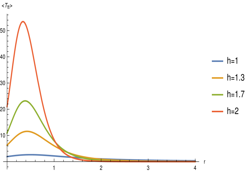
Figure 9: Expectation value of the energy for the state $|\psi_{2,0}\rangle$

Perturbed metric

The ansatz for the metric perturbation is identical to that of $|\psi_{1,0}\rangle$ ((344) , (D.2)). The solutions to Einstein’s equation at the leading order in $G_{N}$ is given by

$$a(r)=\left(8(h+1)r^{2}+8\right)\left(r^{2}+1\right)^{-2h-1}+A(1+r^{2})+B,$$ (355)

$$b(r)=8\left((h+1)r^{2}+1\right)\left(r^{2}+1\right)^{-2h-1}+\frac{1}{2}C\left(r^{2}+1\right)+D,$$ (356)

$$d(r)=8\left(2h^{3}r^{4}+h^{2}\left(r^{2}+2\right)r^{2}+3hr^{2}+h+r^{2}+1\right)\left(r^{2}+1\right)^{-2h-1}+B.$$ (357)

where the constants are found to be $B=-4(2h+2)$, and $A=C=D=0$.

Shift in minimal area

Substituting $rr$ component of the perturbed metric (357) in (327) one can find the minimal area as,

$$\delta A_{|\psi_{2,0}\rangle}= -16G_{N}(h+1)\left[r_{m}\arctan\frac{1}{r_{m}}-1\right]$$

$$+(-2G_{N})\frac{h\sqrt{\pi}\Gamma(2h)}{r_{m}^{4}\Gamma\left(2h+\frac{5}{2}\right)}\bigg{[}(2h+1)r_{m}^{4}\left(r_{m}^{2}+1\right)^{-2h-1}(4h^{2}r_{m}^{2}+h\left(3r_{m}^{2}+7\right)+4)$$

$$+8\left(2h^{2}+3h+1\right)r_{m}^{-4h}\frac{\,{}_{2}F_{1}\left[2(h+1),2h+\frac{5}{2};2h+\frac{7}{2};-\frac{1}{r_{m}^{2}}\right]}{4h+5}\bigg{]}.$$ (358)

In short interval expansion, keeping the analytic term and the leading order non-analytic term we find,

$$\frac{\delta A_{|\psi_{2,0}\rangle}}{4G_{N}}=2(2h+2)(1-\pi x\cot\pi x){-h(2h+1)\frac{\Gamma\left(\frac{3}{2}\right)\Gamma(1+2h)}{\Gamma\left(\frac{3}{2}+2h\right)}\left(\pi x\right)^{4h}}+\cdots.$$ (359)

Bulk entanglement Entropy

From table 2, we note that the Bogoliubov coefficients scale as $\sqrt{h(2h+1)}$ . We substitute $B_{m,n}=\delta_{m,2}\delta_{n,0}$ in (D) to obtain the first order bulk entanglement entropy,

$$S_{\rm bulk}^{(1)}(\Sigma_{A})_{|\psi_{2,0}\rangle}={(\pi x)^{4h}(h(2h+1))\frac{\Gamma(2h+1)\Gamma(\frac{3}{2})}{\Gamma(2h+\frac{3}{2})}}.$$ (360)

From (D) we obtain the second order contribution to the bulk entanglement entropy

$$S_{\rm bulk}^{(2)}(\Sigma_{A})_{|\psi_{2,0}\rangle} =-(\pi x)^{8h}(h(2h+1))^{2}\frac{\Gamma(4h+1)\Gamma(\frac{3}{2})}{\Gamma(4h+\frac{3}{2})}.$$ (361)

Holographic entanglement entropy

Combining (359), (360) and (361) we write down the quantum corrections to holographic entanglement entropy using the FLM formula to second order.

$$S_{\rm FLM}(\Sigma_{A})_{|\psi_{2,0}\rangle}=2(2h+2)(1-\pi x\cot\pi x)-(\pi x)^{8h}(h(2h+1))^{2}\frac{\Gamma(4h+1)\Gamma(\frac{3}{2})}{\Gamma(4h+\frac{3}{2})}.$$ (362)

This is equal to the entanglement entropy of the dual CFT state $L_{-1}^{2}|h\;h\rangle$ as it can be seen by substituting $l=2$ in (2.3).

D.4 Superposition with zero angular momentum

Lastly we consider the simplest superposition with zero angular momentum

$$|{\hat{\upsilon}}\rangle=c_{0}|\psi_{0,0}\rangle+2hc_{1}|\psi_{0,1}\rangle,$$ (363)

which is dual to the following state in the CFT

$$|{\Upsilon}\rangle=c_{0}|h,h\rangle+L_{-1}\bar{L}_{-1}|h,h\rangle.$$ (364)

The CFT computation

We first briefly discuss the CFT analysis since this linear combination is does not fit into the general results for the superposition derived in (76) which dealt with only excitations in the holomorphic sector. The leading correction to the single interval entanglement entropy arises from $n$ 2-points function on the same wedge. From the analysis in section 2.1 we see that the generating function $G(z,\hat{z})$ can be used to obtain the correlator in the holomorphic sector and a similar one but with variables $(z,\hat{z})$ replaced by $\bar{z},\bar{\hat{z}}$ can be used for the anti-holomorphic sector. Therefore we have

$$\Big{\langle}w\circ\partial^{l}\bar{\partial}^{m}{\cal O}(w_{k},\bar{w}_{k})\hat{w}\circ\partial^{l^{\prime}}\bar{\partial}^{m^{\prime}}{\cal O}(\hat{w}_{k},\bar{\hat{w}}_{k})\Big{\rangle} = \left.\partial^{l}_{z}\partial^{l^{\prime}}_{\hat{z}}G(z,\hat{z},n)\right|_{(z,\hat{z})=(0_{k},\hat{0}_{k})}$$

$$\quad\times\left.\partial^{m}_{\bar{z}}\partial^{m^{\prime}}_{{\bar{\hat{z}}}}G(\bar{z},\bar{\hat{z}})\right|_{(\bar{z},\bar{\hat{z}})=(\bar{0}_{k}\bar{\hat{0}}_{k})},$$

where $G$ is defined in (2.1) and its expansion around $n=1$ is given in (25). From evaluating these coefficients we see that to the order $O\big{(}(n-1)\big{)}$ there are no cross terms that depend on products $c_{0}^{*}c_{1}$ and its conjugate. For instance the term proportional to $c_{0}^{*}c_{1}$ in the 2-point funciton will involve a derivative of the kind

$$\left.\partial_{z}G(z,\hat{z},n)\right|_{(z,\hat{z})=(0_{k},\hat{0}_{k})}\times\left.\partial_{\bar{z}}G(\bar{z},\bar{\hat{z}})\right|_{(\bar{z},\bar{\hat{z}})=(\bar{0}_{k}\bar{\hat{0}}_{k})}=O\Big{(}(n-1)^{2}\Big{)}.$$ (366)

Therefore this would not contribute to the entanglement entropy. A similar argument applies for the coefficient $c_{0}c_{1}^{*}$. Then the calculation simplifies to the evaluation of the following coefficients

$$\left.G(z,\hat{z},n)\right|_{(z,\hat{z})=(0_{k},\hat{0}_{k})}\times\left.G(\bar{z},\bar{\hat{z}})\right|_{(\bar{z},\bar{\hat{z}})=(\bar{0}_{k}\bar{\hat{0}}_{k})}=1-(n-1)4h(1-\pi x\cot\pi x)+\Big{(}(n-1)^{2}\Big{)},$$

$$\left.\partial_{z}\partial_{\hat{z}}G(z,\hat{z},n)\right|_{(z,\hat{z})=(0_{k},\hat{0}_{k})}\times\left.\partial_{\bar{z}}\partial_{{\bar{\hat{z}}}}G(\bar{z},\bar{\hat{z}})\right|_{(\bar{z},\bar{\hat{z}})=(\bar{0}_{k}\bar{\hat{0}}_{k})}$$

$$\qquad\qquad\qquad\quad=(2h)^{2}(1-(n-1)4(h+1)(1-\pi x\cot\pi x))+\Big{(}(n-1)\Big{)}^{2}.$$ (367)

Using these results for the two-point function on the same wedge, we can substitute in the expression for the leading behaviour of the $2n$-point function corresponding to the state (364)

$$\frac{{\cal C}_{2n}^{(0)}}{(\langle{\Upsilon}|{\Upsilon}\rangle)^{n}}=1-(n-1)\frac{(4h|c_{0}|^{2}+(2h)^{2}(4h+1))}{|c_{0}|^{2}+(2h)^{2}|c_{1}|^{2})}(1-\pi x\cot\pi x)+O((n-1)^{2}).$$

Let us proceed to evaluate the sub-leading correction to the $2n$-point function for the state $|\Upsilon\rangle$. Going through the same steps as described in section 2.1 and noting that the correlation functions factorize into holomorphic and anti-holomorphic sectors we obtain

$$\frac{{\cal C}^{(1)}_{2n}}{[\langle\Upsilon|\Upsilon\rangle]^{n}}=(n-1)\frac{\Gamma(\frac{3}{2})\Gamma(4h+1)}{\Gamma(4h+\frac{3}{2})}\times\frac{{\cal D}^{2}}{\Big{[}|c_{0}|^{2}+(2h)^{2}|c_{1}|^{2})\Big{]}^{2}}(\pi x)^{8h}+\cdots,$$ (369)

where

$${\cal D} = |c_{0}|^{2}\Big{(}D_{00}(h,2h)\Big{)}^{2}+c_{0}c_{1}^{*}\Big{(}D_{01}(h,2h)\Big{)}^{2}+c_{1}^{*}c_{0}\Big{(}D_{10}(h,2h)\Big{)}^{2}+|c_{1}|^{2}\Big{(}D_{11}(h,2h)^{2}\Big{)}^{2},$$ (370)

$$= |c_{0}+(2h)^{2}c_{1}|^{2}.$$

and we have used the values of $D_{ll^{\prime}}(h,2h)$ from (66) to obtain the second line. The squares of these coefficients occur due to the contributions from both the holomorphic and anti-holomorphic parts of the correlator.

Substituting the results (D.4), (369) into the expression for the entanglement entropy given in (22) we obtain the leading and the sub-leading contribution to the single interval entanglement entropy of the state $|\Upsilon\rangle$

$$\left.S(\rho_{A})\right|_{|\Upsilon\rangle} = \frac{(4h|c_{0}|^{2}+(2h)^{2}(4h+1))}{|c_{0}|^{2}+(2h)^{2}|c_{1}|^{2})}(1-\pi x\cot\pi x)$$

$$-\frac{\Gamma(\frac{3}{2})\Gamma(4h+1)}{\Gamma(4h+\frac{3}{2})}\frac{|c_{0}+(2h)^{2}c_{1}|^{4}}{(|c_{0}|^{2}+(2h)^{2}|c_{1}|^{2}))^{2}}(\pi x)^{8h}+\cdots.$$

Note that the $x$ dependence of the leading term of the linear combination $|\Upsilon\rangle$ is the standard function $(1-\pi x\cot\pi x)$ for the excited states.

Evaluating the FLM formula

The first step in evaluating the FLM formula for the excitation $|\hat{\upsilon}\rangle$ is to obtain the expectation value of the bulk stress tensor in this state. Since the state does not break rotational symmetry, only the diagonal components of the stress tensor expectation values are non-zero. It is sufficient for our purpose to evaluate the following components

Stress tensor components

$$\frac{\langle\upsilon|T_{tt}|\upsilon\rangle}{\langle\upsilon|\upsilon\rangle} =\frac{2h}{\pi(1+r^{2})^{2h+1}\left(|c_{0}|^{2}+(2h)^{2}|c_{1}|^{2}\right)}\Big{[}(2h-1)\left(r^{2}+1\right)^{2}|c_{0}|^{2}$$

$$+4h\left(h\left(2h\left(2(2h-1)r^{2}\left(hr^{2}-1\right)+1\right)+1\right)+1\right)|c_{1}|^{2}$$

$$\left.+h\left(r^{2}+1\right)\left(c_{0}c_{1}^{*}+c_{1}c_{0}^{*}\right)\left((2h-1)r^{2}-1\right)\right)\Big{]},$$

$$\frac{\langle\upsilon|T_{rr}|\upsilon\rangle}{\langle\upsilon|\upsilon\rangle} =\frac{2h}{((2h)^{2}|c_{1}|^{2}+|c_{0}|^{2})\pi(1+r^{2})^{2h+3}}\Big{[}(1+r^{2})^{2}|c_{0}|^{2}$$

$$+4\left(h\left(4hr^{2}\left(hr^{2}-1\right)+3\right)+1\right)|c_{1}|^{2}$$

$$\left.+\left(r^{2}+1\right)\left(c_{0}c_{1}^{*}+c_{1}c_{0}^{*}\right)\left(hr^{2}-1\right)\right)\Big{]}.$$ (372)

Perturbed metric

We use the anstaz in (126) and solve the Einstein’s equations. It is sufficient to discuss the $rr$ component of the metric since it is only this component which determines the minimal area. The solution for $b(r)$ which determines the coefficient of the $rr$ component of the metric is given by

$$b(r)=A-\frac{8h}{\left((2h)^{2}|c_{1}|^{2}+|c_{0}|^{2}\right)\left(r^{2}+1\right)^{2h+1}}$$ (373)

$$\times\Big{[}-\left(r^{2}+1\right)^{2}|c_{0}|^{2}+4h|c_{1}|^{2}\left(4h^{3}r^{4}+2hr^{2}+h+1\right)-4h^{2}\left.r^{2}\left(r^{2}+1\right)\left(c_{0}c_{1}^{*}+c_{1}c_{0}^{*}\right)\right)\Big{]}.$$

We impose the condition that the metric asymptotes to $AdS_{3}$. The constant $A$ is determined by re-writing the metric in the Fefferman-Graham form and demanding that the boundary stress tensor matches with the expectation value of the stress tensor of the CFT in the state $|\Upsilon\rangle$. We obtain

$$A =-\frac{4\left((2h)|c_{0}|^{2}+(2h+2)(2h)^{2}|c_{1}|^{2}\right)}{(2h)^{2}|c_{1}|^{2}+|c_{0}|^{2}}.$$ (374)

Shift in minimal area

We can find the shifted minimal area by using (327) given the $rr$ component which is determined by (373). The leading contribtution together with the non-analytical sub-leading contribution to the minimal area is given by

$$\frac{\delta A_{|\hat{\upsilon}\rangle}}{4G_{N}} = \frac{(4h|c_{0}|^{2}+(2h)^{2}(4h+1))}{|c_{0}|^{2}+(2h)^{2}|c_{1}|^{2}}(1-\pi x\cot\pi x)$$

$$-\frac{\Gamma(2h+1)\Gamma(\frac{3}{2})}{\Gamma(2h+\frac{3}{2})}\frac{|c_{0}+(2h)^{2}c_{1}|^{2}}{|c_{0}|^{2}+(2h)^{2}|c_{1}|^{2}}(\pi x)^{4h}+\cdots.$$

Bulk entanglement entropy

From table 2, we note that the Bogoliubov coefficients scale as

$$\lim_{\eta\rightarrow\infty}\alpha_{0,1;\omega,k}=2h\lim_{\eta\rightarrow\infty}\alpha_{0,0,\omega,k},\qquad\lim_{\eta\rightarrow\infty}\beta_{0,1;\omega,k}=2h\lim_{\eta\rightarrow\infty}\beta_{0,0,\omega,k}.$$ (376)

For the state $|\hat{\upsilon}\rangle$ the non-zero coefficients for the $B$’s are given by

$$B_{0,0}=\frac{c_{0}}{\sqrt{|c_{0}|^{2}+(2h)^{2}|c_{1}|^{2}}},\qquad B_{0,1}=\frac{2hc_{1}}{\sqrt{|c_{0}|^{2}+(2h)^{2}|c_{1}|^{2}}}.$$ (377)

Substituting the scaling relation (376) and the values of $B$’s into the expression for the first order bulk entanglement entropy (328), we obtain

$$\left.S^{(1)}_{\rm bulk}(\Sigma_{A})\right|_{|\hat{\upsilon}\rangle}=\frac{\Gamma(2h+1)\Gamma(\frac{3}{2})}{\Gamma(2h+\frac{3}{2})}\frac{|c_{0}+(2h)^{2}c_{1}|^{2}}{|c_{0}|^{2}+(2h)^{2}|c_{1}|^{2}}(\pi x)^{4h}.$$ (378)

Note that this non-analytic term from the first order bulk entanglement entropy precisely cancels the corresponding term in the minimal area (D.4) as expected from the gravitational Gauss law. For the second order contribution to the bulk entanglement entropy we use the general expression in (D) and obtain

$$\left.S^{(2)}_{\rm bulk}(\Sigma_{A})\right|_{|\upsilon\rangle}=-\frac{\Gamma(\frac{3}{2})\Gamma(4h+1)}{\Gamma(4h+\frac{3}{2})}\frac{|c_{0}+(2h)^{2}c_{1}|^{4}}{(|c_{0}|^{2}+(2h)^{2}|c_{1}|^{2})^{2}}(\pi x)^{8h}+\cdots.$$ (379)

Now summing up the contributions from (378), (379) and the minimal area (D.4) we obtain the entanglement entropy in gravity using the FLM Formula.

$$\left.S_{\rm FLM}(\rho_{A})\right|_{|\upsilon\rangle} = \frac{(4h|c_{0}|^{2}+(2h)^{2}(4h+1))}{|c_{0}|^{2}+(2h)^{2}|c_{1}|^{2}}(1-\pi x\cot\pi x)$$

$$-\frac{\Gamma(\frac{3}{2})\Gamma(4h+1)}{\Gamma(4h+\frac{3}{2})}\frac{|c_{0}+(2h)^{2}c_{1}|^{4}}{(|c_{0}|^{2}+(2h)^{2}|c_{1}|^{2})^{2}}(\pi x)^{8h}+\cdots.$$

This precisely agrees with the CFT answer computed in (D.4).

References

- (1) S. Ryu and T. Takayanagi, Holographic derivation of entanglement entropy from AdS/CFT, Phys. Rev. Lett. 96 (2006) 181602 [hep-th/0603001].
- (2) T. Faulkner, A. Lewkowycz and J. Maldacena, Quantum corrections to holographic entanglement entropy, JHEP 11 (2013) 074 [1307.2892].
- (3) N. Engelhardt and A.C. Wall, Quantum Extremal Surfaces: Holographic Entanglement Entropy beyond the Classical Regime, JHEP 01 (2015) 073 [1408.3203].
- (4) X. Dong and A. Lewkowycz, Entropy, Extremality, Euclidean Variations, and the Equations of Motion, JHEP 01 (2018) 081 [1705.08453].
- (5) D.L. Jafferis, A. Lewkowycz, J. Maldacena and S.J. Suh, Relative entropy equals bulk relative entropy, JHEP 06 (2016) 004 [1512.06431].
- (6) X. Dong, D. Harlow and A.C. Wall, Reconstruction of Bulk Operators within the Entanglement Wedge in Gauge-Gravity Duality, Phys. Rev. Lett. 117 (2016) 021601 [1601.05416].
- (7) T. Faulkner and A. Lewkowycz, Bulk locality from modular flow, JHEP 07 (2017) 151 [1704.05464].
- (8) S. Hawking, Stable and generic properties in general relativity, Gen. Rel. Grav. 1 (1971) 393.
- (9) J.D. Bekenstein, Black holes and entropy, Phys. Rev. D 7 (1973) 2333.
- (10) S.W. Hawking, Particle Creation by Black Holes, Commun. Math. Phys. 43 (1975) 199.
- (11) V.E. Hubeny, M. Rangamani and T. Takayanagi, A Covariant holographic entanglement entropy proposal, JHEP 07 (2007) 062 [0705.0016].
- (12) T. Barrella, X. Dong, S.A. Hartnoll and V.L. Martin, Holographic entanglement beyond classical gravity, JHEP 09 (2013) 109 [1306.4682].
- (13) B. Chen and J.-J. Zhang, On short interval expansion of Rényi entropy, JHEP 11 (2013) 164 [1309.5453].
- (14) S. Datta and J.R. David, Rényi entropies of free bosons on the torus and holography, JHEP 04 (2014) 081 [1311.1218].
- (15) M. Headrick, A. Maloney, E. Perlmutter and I.G. Zadeh, Rényi entropies, the analytic bootstrap, and 3D quantum gravity at higher genus, JHEP 07 (2015) 059 [1503.07111].
- (16) T. Miyagawa, N. Shiba and T. Takayanagi, Double-Trace Deformations and Entanglement Entropy in AdS, Fortsch. Phys. 64 (2016) 92 [1511.07194].
- (17) S. Sugishita, Entanglement entropy for free scalar fields in AdS, JHEP 09 (2016) 128 [1608.00305].
- (18) A. Belin, N. Iqbal and S.F. Lokhande, Bulk entanglement entropy in perturbative excited states, SciPost Phys. 5 (2018) 024 [1805.08782].
- (19) C.A. Agón, S.F. Lokhande and J.F. Pedraza, Local quenches, bulk entanglement entropy and a unitary Page curve, JHEP 08 (2020) 152 [2004.15010].
- (20) B.G. Chowdhury and J.R. David, Entanglement in descendants, JHEP 02 (2022) 003 [2108.00898].
- (21) T. Pálmai, Excited state entanglement in one dimensional quantum critical systems: Extensivity and the role of microscopic details, Phys. Rev. B 90 (2014) 161404 [1406.3182].
- (22) P. Caputa and A. Veliz-Osorio, Entanglement constant for conformal families, Phys. Rev. D 92 (2015) 065010 [1507.00582].
- (23) L. Taddia, F. Ortolani and T. Pálmai, Renyi entanglement entropies of descendant states in critical systems with boundaries: conformal field theory and spin chains, J. Stat. Mech. 1609 (2016) 093104 [1606.02667].
- (24) E.M. Brehm and M. Broccoli, Correlation functions and quantum measures of descendant states, JHEP 04 (2021) 227 [2012.11255].
- (25) R.M. Wald, Black hole entropy is the Noether charge, Phys. Rev. D 48 (1993) R3427 [gr-qc/9307038].
- (26) V. Iyer and R.M. Wald, Some properties of Noether charge and a proposal for dynamical black hole entropy, Phys. Rev. D 50 (1994) 846 [gr-qc/9403028].
- (27) P. Caputa and D. Ge, Entanglement and geometry from subalgebras of the Virasoro algebra, JHEP 06 (2023) 159 [2211.03630].
- (28) M. Banados, Three-dimensional quantum geometry and black holes, AIP Conf. Proc. 484 (1999) 147 [hep-th/9901148].
- (29) G. Sárosi and T. Ugajin, Relative entropy of excited states in two dimensional conformal field theories, JHEP 07 (2016) 114 [1603.03057].
- (30) E. Perlmutter, Virasoro conformal blocks in closed form, JHEP 08 (2015) 088 [1502.07742].
- (31) P. Calabrese, J. Cardy and E. Tonni, Entanglement entropy of two disjoint intervals in conformal field theory II, J. Stat. Mech. 1101 (2011) P01021 [1011.5482].
- (32) J.M. Maldacena and A. Strominger, AdS(3) black holes and a stringy exclusion principle, JHEP 12 (1998) 005 [hep-th/9804085].
- (33) H. Casini, M. Huerta and R.C. Myers, Towards a derivation of holographic entanglement entropy, JHEP 05 (2011) 036 [1102.0440].
- (34) A. Hamilton, D.N. Kabat, G. Lifschytz and D.A. Lowe, Holographic representation of local bulk operators, Phys. Rev. D 74 (2006) 066009 [hep-th/0606141].
- (35) A. Almheiri, X. Dong and D. Harlow, Bulk Locality and Quantum Error Correction in AdS/CFT, JHEP 04 (2015) 163 [1411.7041].
- (36) N. Lashkari and M. Van Raamsdonk, Canonical Energy is Quantum Fisher Information, JHEP 04 (2016) 153 [1508.00897].
- (37) N. Lashkari, J. Lin, H. Ooguri, B. Stoica and M. Van Raamsdonk, Gravitational positive energy theorems from information inequalities, PTEP 2016 (2016) 12C109 [1605.01075].
- (38) G. Sárosi and T. Ugajin, Relative entropy of excited states in conformal field theories of arbitrary dimensions, JHEP 02 (2017) 060 [1611.02959].
- (39) A. Belin, N. Iqbal and J. Kruthoff, Bulk entanglement entropy for photons and gravitons in AdS3, SciPost Phys. 8 (2020) 075 [1912.00024].
- (40) A. Belin and S. Colin-Ellerin, Bootstrapping quantum extremal surfaces. Part I. The area operator, JHEP 11 (2021) 021 [2107.07516].
- (41) J.R. David and J. Mukherjee, Entanglement entropy of gravitational edge modes, JHEP 08 (2022) 065 [2201.06043].
- (42) W. Donnelly, L. Freidel, S.F. Moosavian and A.J. Speranza, Matrix Quantization of Gravitational Edge Modes, JHEP 05 (2027) 163 [2212.09120].
- (43) M. Grewal, Y.T.A. Law and K. Parmentier, Black hole horizon edge partition functions, JHEP 06 (2023) 025 [2211.16644].
- (44) J. Mukherjee, Entanglement entropy and the boundary action of edge modes, 2310.14690.
- (45) A. Ball, A. Law and G. Wong, Dynamical Edge Modes and Entanglement in Maxwell Theory, 2403.14542.
- (46) T.G. Mertens, J. Simón and G. Wong, A proposal for 3d quantum gravity and its bulk factorization, JHEP 06 (2023) 134 [2210.14196].
- (47) E. Joung, P. Narayan and J. Yoon, Gravitational Edge Mode in Asymptotically AdS2: JT Gravity Revisited, 2304.06088.
- (48) K. Lee, A. Sivakumar and J. Yoon, Gravitational Edge Mode in Jackiw-Teitelboim Supergravity, 2403.17182.
- (49) J. Cardy and E. Tonni, Entanglement hamiltonians in two-dimensional conformal field theory, J. Stat. Mech. 1612 (2016) 123103 [1608.01283].
- (50) V. Balasubramanian and P. Kraus, A Stress tensor for Anti-de Sitter gravity, Commun. Math. Phys. 208 (1999) 413 [hep-th/9902121].
- (51) S. de Haro, S.N. Solodukhin and K. Skenderis, Holographic reconstruction of space-time and renormalization in the AdS / CFT correspondence, Commun. Math. Phys. 217 (2001) 595 [hep-th/0002230].