Stronger Speed Limit for Observables: Tight bound for Capacity of Entanglement,
Modular Hamiltonian and Charging of Quantum Battery

Abstract

How fast an observable can evolve in time is answered by so-called the ”observable speed limit”. Here, we prove a stronger version of the observable speed limit and show that the previously obtained bound is a special case of the new bound. The stronger quantum speed limit for the state also follows from the stronger quantum speed limit for observables (SQSLO). We apply this to prove a stronger bound for the entanglement rate using the notion of capacity of entanglement (the quantum information theoretic counterpart of the heat capacity) and show that it outperforms previous bounds. Furthermore, we apply the SQSLO for the rate of modular Hamiltonian and in the context of interacting qubits in a quantum battery. These illustrative examples reveal that the speed limit for the modular energy and the time required to charge the battery can be exactly predicted using the new bound. This shows that for estimating the charging time of quantum battery SQSLO is actually tight, i.e. it saturates. Our findings can have important applications in quantum thermodynamics, the complexity of operator growth, predicting the time rate of quantum correlation growth and quantum technology, in general.

I Introduction

Since the inception of scientific explorations, time has remained a paramount and fundamental notion in the study of physical systems. However, understanding time presents a considerable challenge, as it is not an operator but rather a parameter. New insights on the nature of time emerged after the formulation of the geometric uncertainty relation between energy fluctuation and time, imposing limitations on the rate at which a quantum system evolves. This concept was later formalized as the Quantum Speed Limit (QSL) Mandelstam and Tamm (1945); Anandan and Aharonov (1990), which delineates the minimal time required for the evolution of a quantum system. Additionally, another speed limit was identified for quantum state evolution, which incorporates the average energy in the ground state of the Hamiltonian  Pati (1991); Margolus and Levitin (1998). The QSL depends on the shortest path connecting the initial and final states of a given quantum system which depends on the fluctuation in the Hamiltonian and thus provides crucial insights into the dynamics of quantum processes.

During the nascent stages of research, the bounds of the QSL were primarily established for the unitary dynamics of pure states for quantum systems Mandelstam and Tamm (1945); Anandan and Aharonov (1990); Pati (1991); Margolus and Levitin (1998); Levitin and Toffoli (2009); Gislason et al. (1985); Eberly and Singh (1973); Bauer and Mello (1978); Bhattacharyya (1983); Leubner and Kiener (1985); Vaidman (1992); Uhlmann (1992); Uffink (1993); Pfeifer and Fröhlich (1995); Horesh and Mann (1998); Pati (1999); Söderholm et al. (1999); Andrecut and Ali (2004); Gray and Vogt (2005); Zieliński and Zych (2006); Andrews (2007); Yurtsever (2010); Shuang-Shuang et al. (2010); Poggi et al. (2013). Subsequently, researchers delved into investigating QSL within the framework of unitary dynamics for mixed states Kupferman and Reznik (2008); Jones and Kok (2010); Chau (2010); Deffner and Lutz (2013); Fung and Chau (2014); Andersson and Heydari (2014); Mondal et al. (2016); Mondal and Pati (2016); Deffner and Campbell (2017a); Campaioli et al. (2018a). The significance of QSL extends beyond theoretical explorations as it plays a pivotal role in the advancement of quantum technologies and devices, among other applications. Indeed, QSL finds diverse applications, including but not limited to, quantum computing Ashhab et al. (2012), quantum thermodynamics Mukhopadhyay et al. (2018); Funo et al. (2019), quantum control theory Caneva et al. (2009); Campbell and Deffner (2017), quantum metrology Campbell et al. (2018), and beyond.

Later, following the discovery of the stronger uncertainty relation Ref. Maccone and Pati (2014), a more robust QSL was unveiled Thakuria and Pati (2022), which presented a tighter bound than the previously established MT and ML bounds. These advancements were made within the Schrödinger picture, where the state vector evolves over time. Subsequently, the exploration of QSL within the Heisenberg picture where observables evolve in time rather than the state, gathered interest.

Henceforth, leveraging the Robertson-Heisenberg uncertainty relation within the Heisenberg picture, a novel QSL bound was established, which is termed as the Quantum Speed Limit for observables (QSLO) Mohan and Pati (2022). This development prompted a natural inquiry: could we derive another bound using the stronger uncertainty relation? This question arises because the SQSL is already tighter than the MT bound, and while the QSLO is approximately equally as tight as the MT bound, there remains a need for a tighter bound for observables in the Heisenberg picture. Indeed, not only have we derived this new stronger bound, but have shown that it gives a significant improvement over QSLO while examining few prominent examples provided in this paper.

Entanglement is considered a very useful resource in information-processing tasks. Hence over the years, how to create and quantify entanglement has been a subject of major exploration Horodecki et al. (2009); Das et al. (2016). The creation of quantum entanglement between two particles depends upon the choice of the initial state and suitable non-local interaction between them, but the designing of suitable interacting Hamiltonian is not always easy, which renders the production of entanglement a non-trivial task. Thus, for a given non-local Hamiltonian, what can be the best way to utilize this Hamiltonian to create entanglement. One way to answer this query, is by making use of the capacity of entanglement that was originally proposed to characterize topologically ordered states in the context of Kitaev model de Boer et al. (2019a). For a given pure bipartite entangled state $\rho_{AB}$, the capacity of entanglement is defined as the second cumulant of the entanglement spectrum, i.e., associated with the reduced density matrix, with $\{\lambda_{i}\}^{\prime}$s, the eigenvalues of the reduced density matrix of any one of the subsystem, the capacity of entanglement $C_{E}$ is defined as the second cumulant of this entanglement spectrum, i.e; $C_{E}=\sum_{i}\lambda_{i}{\rm log}^{2}\lambda_{i}-S_{EE}^{2}$, where $S_{EE}=-\sum_{i}\lambda_{i}{\rm log}\lambda_{i}$ is the well-known entanglement entropy. $C_{E}$ is similar in form to the heat capacity of thermal systems and can be thought of as the variance of the distribution of $-\log\lambda_{i}$ with probability $\lambda_{i}$ and hence contains information about the width of the eigenvalue distribution of reduced density matrix. It was shown in Ref. Shrimali et al. (2022) that the quantum speed limit for creating the entanglement depends inversely on the fluctuation in the non-local Hamiltonian as well as on the average of the square root of the capacity of entanglement. It was, thus, inferred that the more the capacity of entanglement, the shorter the time duration system may take to produce the desired amount of entanglement.

Our first illustration involves readdressing the entanglement rate which was bounded by fluctuation in the non-local Hamiltonian and the capacity of entanglement as defined in Ref. de Boer et al. (2019b). It is to be seen whether we can achieve a tighter bound for entanglement generation or degradation with the stronger uncertainty relation. If so, what can be the physical implication for the new expression, and under what choice of parameters we can achieve a tighter bound for a greater duration? Furthermore, a similar object was studied under the Heisenberg picture and the subsequent bound was interpreted in the form of the generation of modular energy, defined in the present context as a mean of composite modular Hamiltonian. Needless to say, the notion of capacity of entanglement has applications in diverse areas of physics ranging from condensed matter systems Laflorencie (2016) to conformal field theories de Boer et al. (2019b); Yao and Qi (2010), and alike.

For the final example case, we analyse the ergotropy and bound on the charging process of quantum batteries. The various traditional batteries we make use of such as Lithium-ion, alkaline, and lead-acid batteries operate based on electrochemical reactions involving the movement of electrons between two electrodes through electrolytes. The performance of these batteries depends on factors like electrolyte composition, electrode materials, and overall design. The Quantum batteries (QBs) represent a new frontier, grounded in quantum mechanical principles such as tunneling effects, entanglement, qubit-based technologies, and more Alicki and Fannes (2013). Theoretical models propose that these batteries can leverage quantum superposition and entanglement to store and recover energy, offering enhanced efficiency compared to conventional batteries Binder et al. (2015); Campaioli et al. (2017); Rossini et al. (2020); Gyhm et al. (2022); Gyhm and Fischer (2024). However, despite their potential advantages, QBs are still in the early stages of development due to technological limitations. Numerous challenges, including issues related to stability, scalability, and practical implementation, need to be addressed for their widespread usage Julià-Farré et al. (2020); Campaioli et al. (2023).

The QB model comprises two essential components: a battery charger and a battery holder. However, energy loss is also accounted for in the subsequent stages, achievable by isolating the quantum system from the environment, treated as a dissipation-less subsystem. The effective coupling of the battery holder with the battery charger is crucial for energy acquisition. The focus of recent theoretical research has been on exploring basic bipartite state models and other related models in the realm of quantum batteries Andolina et al. (2018); Le et al. (2018); Zhang et al. (2019); Barra (2019); Santos et al. (2019); Andolina et al. (2019); Crescente et al. (2020a); Santos et al. (2020); Santos (2021); Dou et al. (2022); Barra et al. (2022); Carrasco et al. (2022); Shaghaghi et al. (2022); Rodríguez et al. (2023); Santos et al. (2023); Kamin et al. (2023); Downing and Ukhtary (2023); Hadipour et al. (2023). Theoretical evidence already supports the notion that in a collective charging scheme, QBs can demonstrate accelerated charging leveraging quantum correlations Binder et al. (2015); Campaioli et al. (2017); Kamin et al. (2020a). Presently, diverse models of QBs have been proposed, including quantum cavities, spin chains, the Sachdev-Ye-Kitaev model and quantum oscillators Pirmoradian and Mølmer (2019); Zhang and Blaauboer (2023); Crescente et al. (2020b); Joshi and Mahesh (2022); Julià-Farré et al. (2020); Mohan and Pati (2021); Niedenzu et al. (2018); Andolina et al. (2019); Ferraro et al. (2018); Zhao et al. (2021); Rossini et al. (2019); Zakavati et al. (2021); Zhao et al. (2022). However, experimental investigations are limited, with fewer models explored, such as the cavity-assisted charging of an organic quantum battery Quach et al. (2022). In this article, we take the example of entanglement based QBs under different charging regimes. It is examined whether stronger quantum speed limit for observables (SQSLO) gives any significant improvement over existing QSLO Mohan and Pati (2022); Carabba et al. (2022) for charging time.

This paper is organised as follows. In Section II, we discuss all the basic concepts utilized in this paper. Subsequently, in Section III, we derive the SQSLO bound by employing a stronger uncertainty relation and compare it with other previously established bounds. In the next Section IV, we have given the SQSL for states and demonstrated a better bound for entanglement generation with capacity of entanglement. Following this, in Section V, we present two applications of the QSLO bound for the modular energy and charging time of the quantum battery. Finally, in Section VI, we conclude our paper.

II Definitions and Relations

Stronger Uncertainty Relation: Unlike classical system, where all observables can be measured with arbitrary accuracy, the same is not true for quantum systems. For a given quantum state there are restrictions on the results of the measurements of non-commuting observables. The uncertainty relation captures such a restriction for two incompatible observables.

The Heisenberg-Robertson uncertainty relation provides a lower bound by merely yielding the product of two variances of observables based on their commutator. This proves that it is impossible to prepare a quantum state for which variances of two non-commuting observables can be arbitrarily reduced simultaneously. In contrast, a stronger uncertainty relation offers a more comprehensive approach by considering the sum of variances. This approach ensures that the lower bound remains non-trivial, especially when dealing with two observables that are incompatible within the state of the system. Thus, it provides a more nuanced understanding of uncertainty, particularly in cases where traditional relations fall short. However, we will not be using the sum form of the stronger uncertainty relation. One of the stronger uncertainty relation in the product form as given in Maccone and Pati (2014) has the form

$$\Delta A\Delta B\geq\pm\frac{i}{2}\frac{\langle[A,B]\rangle}{\left(1-\frac{1}{2}\left|\langle\Psi^{\perp}|\frac{A}{\Delta A}\mp i\frac{B}{\Delta B}|\Psi\rangle\right|^{2}\right)},$$ (1)

where $A$ and $B$ are two incompatible observables with $\Delta A=\sqrt{\langle A^{2}\rangle-\langle A\rangle^{2}},\hskip 2.84544pt\Delta B=\sqrt{\langle B^{2}\rangle-\langle B\rangle^{2}}$, and the averages are defined in the state $|\Psi\rangle$ for the given quantum system. This Eqn. (1) can be reduced to the Heisenberg-Robertson uncertainty relation when it minimizes the lower bound over $|\Psi^{\perp}\rangle$ and becomes an equality when maximizes it. The above relation is stronger than the standard Heisenberg-Robertson uncertainty relation. We will be using this to prove our stronger quantum speed limit for observable.

Capacity of entanglement: Let us consider a composite system $AB$ with pure state $|\Psi\rangle_{AB}$. The amount of entanglement between subsystems $A$ and $B$ can be quantified via the entanglement entropy which is defined as the von Neumann entropy of the reduced density operator $\rho_{A}=\sum_{n}\lambda_{n}\ket{\psi_{n}}_{A}\bra{\psi_{n}}$ (or $\rho_{B}$), i.e.,

$$S_{EE}=S(\rho_{A})=-\operatorname{tr}(\rho_{A}\log\rho_{A})=-\sum_{n}\lambda_{n}\log\lambda_{n}$$ (2)

which is invariant under local unitary transformations on $\rho_{A}$. The von Neumann entropy vanishes when density operator $\rho_{A}$ is a pure state. For a completely mixed density operator, the von Neumann entropy attains its maximum value of $\rm\log d_{A}$, where $\rm d_{A}=dim(\cal{H}_{A})$.

For any density operator $\rho_{A}$ associated with quantum system $A$, we can define a formal “Hamiltonian” $K_{A}$, called the modular Hamiltonian, with respect to which the density operator $\rho_{A}$ is a Gibbs like state (with $\beta=1$)

$$\rho_{A}=\frac{e^{-K_{A}}}{Z},$$

where $Z=\operatorname{tr}(e^{-K_{A}}).$ Note that any density matrix can be written in this form for some choice of Hermitian operator $K_{A}$. With slight adjustments in the above equation, the modular Hamiltonian $K_{A}$ can be written as $K_{A}=-\log\rho_{A}$. In this case, the entanglement entropy of the system is equivalent to the thermodynamic entropy of a system described by Hamiltonian $K_{A}$ (with $\beta=1$). Writing in terms of modular Hamiltonian $K_{A}=-\log\rho_{A}$, the entanglement entropy becomes the expectation value of the modular Hamiltonian

$$S_{EE}=-\operatorname{tr}(\rho_{A}\log\rho_{A})=\operatorname{tr}(\rho_{A}K_{A})=\langle K_{A}\rangle\,.$$ (3)

The capacity of entanglement is another information-theoretic quantity that has gained some interest in recent time Caputa et al. (2022). It is defined as the variance of the modular Hamiltonian $K_{A}$ de Boer et al. (2019b) in the state $\ket{\Psi}_{AB}$ and can be expressed as

$$C_{E}(\rho_{A}) =\bra{\Psi}(K_{A}\otimes\mathcal{I}_{B})^{2}\ket{\Psi}-\bra{\Psi}(K_{A}\otimes\mathcal{I}_{B})\ket{\Psi}^{2}$$

$$=\operatorname{tr}[\rho_{A}(-\log\rho_{A})^{2}]-[\operatorname{tr}(-\rho_{A}\,\log\rho_{A})]^{2}$$ (4)

$$=\operatorname{tr}[\rho_{A}K_{A}^{2}]-[\operatorname{tr}(\rho_{A}K_{A})]^{2}$$

$$=\langle K_{A}^{2}\rangle-\langle K_{A}\rangle^{2}=\Delta K_{A}^{2}.$$ (5)

The capacity of entanglement has also been defined in terms of variance of the relative surprisal between two density matrices $V(\rho||\sigma)$:

$$V(\rho||\sigma)=\operatorname{tr}\left(\rho(\log(\rho)-\log(\sigma))^{2}\right)-D(\rho||\sigma)^{2}.$$ (6)

Here, if one of the density matrices becomes maximally mixed (i.e., either $\rho$ or $\sigma$ becomes $\mathcal{I}/d$), then the variance of the relative surprisal becomes the capacity of entanglement. For further details and properties of capacity of entanglement, readers are advised to go through Ref. Pandey et al. (2023).

Extractable work from quantum batteries: Let the quantum system representing the battery be of dimension $d$ with the corresponding Hilbert space $\mathcal{H}$. We further pick a standard basis for describing the system Hamiltonian

$$H=\sum_{j=1}^{d}h_{j}|j\rangle\langle j|\hskip 7.11317pt{\rm with}\hskip 7.11317pth_{j+1}>h_{j},$$ (7)

where the assumption is that the energy levels are non-degenerate.

To extract the energy from the battery, the time-dependent fields that are used can be described as $V(t)=V^{\dagger}(t)$ where such fields are switched on for time interval $0\geq t\geq\tau$. The initial state of the battery is described by a density matrix $\rho$ which is evolved from the Liouville equation

$$\frac{d}{dt}\rho(t)=-i[H+V(t),\rho(t)],\hskip 8.5359pt\rho(0)=\rho.$$ (8)

The work extraction by this procedure is then

$$W={\rm tr}(\rho H)-{\rm tr}(\rho(\tau)H),$$ (9)

where time evolved state is given as $\rho(\tau)=U(\tau)\hskip 2.84544pt\rho\hskip 2.84544ptU^{\dagger}(\tau)$.

Further, through a proper choice of $V$, any unitary $U$ can be obtained for $U(\tau)$. Therefore the maximal amount of extractable work, called ergotropy, can be defined as

$$W_{max}:={\rm tr}(\rho H)-\min{\rm tr}(U\rho U^{\dagger}H),$$ (10)

where the minimum is taken over all unitary transformations of $\mathcal{H}$.

III Stronger QSL for Observables (SQSLO)

III.1 Derivation of Stronger Quantum Speed Limit for Observables

Let us consider a quantum system with a state vector $|\Psi\rangle\in\mathcal{H}^{N}$. In the Heisenberg picture, we can imagine that the operators representing the observables evolve in time, while the vectors in the Hilbert space (quantum states) remain independent of time. This is opposite to the Schrödinger picture, where the observables are independent of time and the states evolve in time. In the Heisenberg picture, each self-adjoint operator evolves in time according to the operator-valued differential equation.

As we are dealing with the Heisenberg picture, the observable $O(t)$undergoes an unitary evolution as given by the Heisenberg equation of motion

$$i\hbar\frac{dO(t)}{dt}=[O(t),H],$$ (11)

where $H$ is the Hamiltonian operator of the system, and where $[O,H]$ is the commutator. If $O(t)$ commutes with the Hamiltonian, then it remains constant in time. In this section, we aim to derive a more stringent QSL bound for observables, surpassing the previously obtained limit. This bound stems from the stronger uncertainty relation, applicable to any two incompatible observables $A(t)$ and $B(t)$ in the Heisenberg picture. This is given by

$$\Delta A(t)\hskip 2.84544pt\Delta B(t)\hskip 2.84544pt(1-R(t))\geq\pm\frac{i}{2}\langle\Psi|[A(t),B(t)]|\Psi\rangle,$$ (12)

where

$$R(t)=\frac{1}{2}\left|\langle\Psi^{\perp}|\frac{A(t)}{\Delta A(t)}\mp i\frac{B(t)}{\Delta B(t)}|\Psi\rangle\right|^{2},$$ (13)

$\Delta A(t)$ = $\sqrt{\langle A(t)^{2}\rangle-\langle A(t)\rangle^{2}}$, $\Delta B(t)$ = $\sqrt{\langle B(t)^{2}\rangle-\langle B(t)\rangle^{2}}$, $|\Psi\rangle$ is the state of the system in which averages are calculated and $|\Psi^{\perp}\rangle$ is the orthogonal state to $|\Psi\rangle$. We will prove that the bound obtained from the above equation is tighter than the existing bound $T_{QSLO}$ which was derived by using Robertson uncertainty relation.

Now, consider the desired observable, denoted as $A=O(t)$, and an another operator, $B=H$. Using the stronger uncertainty relation, we can obtain

$$\Delta O(t)\hskip 2.84544pt\Delta H\hskip 2.84544pt(1-R(t))\geq\frac{\hbar}{2}\left|\frac{d\langle O(t)\rangle}{dt}\right|.$$ (14)

From the above expression, we obtain the stronger quantum speed limit for observable (SQSLO) as given by

$$T\geq T_{SQSL}^{O}=\frac{\hbar}{2\Delta H}\int_{0}^{T}\frac{|d\langle O(t)\rangle|}{\Delta O(t)\hskip 2.84544pt\eta(t)},$$ (15)

where $\eta(t)$ = $(1-R(t))$, $\Delta O(t)$ = $\sqrt{\langle O(t)^{2}\rangle-\langle O(t)\rangle^{2}}$ and $\Delta H$ = $\sqrt{\langle H^{2}\rangle-\langle H\rangle^{2}}$. This SQSLO can be written as

$$T_{SQSL}^{O}=\frac{\hbar}{2\Delta H}\frac{|\langle O(T)\rangle-\langle O(0)\rangle|}{\langle\langle\Delta O(t)\hskip 2.84544pt\eta(t)\rangle\rangle_{T}},$$ (16)

where $\langle\langle\Delta O(t)\hskip 2.84544pt\eta(t)\rangle\rangle_{T}$ = $\frac{1}{T}\int_{0}^{T}\Delta O(T)\hskip 2.84544pt\eta(t)dt$, is the time average of the quantity $\Delta O(t)\hskip 2.84544pt\eta(t)$ Pati et al. (2023).

Using Eqn.(14), in an alternative way, we can write SQSLO as

$$T\geq\frac{\hbar\hskip 2.84544pt\Lambda(T)}{2\Delta H}\int_{0}^{T}\frac{|d\langle O(t)\rangle|}{\Delta O(t)},$$ (17)

where $\Lambda(T)=\frac{1}{1-\overline{R}(t)}$, with $\overline{R}(t)=\frac{1}{T}\int_{0}^{T}R(t)\hskip 2.84544ptdt$.

Now, we can show that the previously derived bound of the QSLO Mohan and Pati (2022) follows from the stronger QSLO. This will ensure that SQSLO is indeed tighter than QSLO. As evident from Eqn. (15), an additional factor of $\eta(t)=1-R(t)$ is present in SQSLO, with $0\leq R(t)\leq 1\hskip 2.84544pt\forall\hskip 2.84544ptt$, we have $\eta(t)\in[0,1]$. This results in the final expression

$$T\geq\frac{\hbar}{2\Delta H}\int_{0}^{T}\frac{|d\langle O(t)\rangle|}{\Delta O(t)\eta(t)}\geq\frac{\hbar}{2\Delta H}\int_{0}^{T}\frac{|d\langle O(t)\rangle|}{\Delta O(t)}.$$ (18)

Therefore, we have

$$T\geq T_{SQSL}^{O}\geq T_{QSL}^{O}$$ (19)

This shows that indeed SQSLO is tighter than QSLO.

IV Stronger QSL for states and Entanglement Capacity

In this section, we delve into the relationship between SQSL for observables and SQSL concerning states. Notably, SQSL for state emerges as a distinctive instance within the broader framework of SQSL for observable, when we consider the observable as the projector of the initial state. For realising that, let us consider a quantum system with an initial state $|\Psi\rangle=\sum_{i}c_{i}|i\rangle$. We continue with the observable taking the form of a projector, i.e., $O(0)=P$. Consequently, the probability of finding the system in state $|i\rangle$ at time $t=0$ becomes $|c_{i}|^{2}$, upon performing measurement with projector defined as $P=|i\rangle\langle i|$. Now we wish to study the bound on speed limit for the projector for the quantum system evolving a state $\ket{i}$ unitarily in time. Using Eqn. (17) in an alternative way, we can express the quantum speed limit for the projector as given by

$$T\geq\frac{\hbar\hskip 2.84544pt\Lambda(T)}{2\Delta H}\int_{0}^{T}\frac{|d\langle P(t)\rangle|}{\Delta P(t)},$$ (20)

where $P(t)$ = $U(t)P(0)U(t)^{\dagger}$ and $\langle P(t)\rangle$ = $p(t)$ is the probability of the quantum system in state $|i\rangle$ at some later time $t$.

The above bound can be expressed as

$$T\geq\frac{\hbar\Lambda(T)}{\Delta H}\left|\arcsin(\sqrt{p(T)})-\arcsin(\sqrt{p(0)})\right|,$$ (21)

where $\Lambda(T)=\frac{1}{1-\overline{R}(t)}$, with $\overline{R}(t)=\frac{1}{T}\int_{0}^{T}R(t)\hskip 2.84544ptdt$. Now if we choose $p(0)=1$, i.e, $\ket{\Psi}=\ket{i}$, then the above inequality results in the following bound

$$T\geq\frac{\hbar\Lambda(T)}{\Delta H}\arccos(\sqrt{p(T)}).$$ (22)

This is equivalent to the stronger speed limit for the state obtained in Ref. Mohan and Pati (2022). As we know the Mandelstam and Tamm bound is a special case of the stronger speed limit for the state, we can say that the stronger speed limit for the state and MT bound, both are special cases of the stronger quantum speed limit for the observable. Thus, our result unifies the previous known bounds on the observable and state.

Next, we apply the SQSL for state to provide stronger bound for the entanglement rate using capacity of entanglement.

Improved Bounds on Rate of Entanglement through capacity of entanglement using SQSL for states

The dynamics of entanglement under two-qubit nonlocal Hamiltonian has been adressed in Ref. Dür et al. (2001). Further, the inquiry on capacity of entanglement for two-qubit non-local Hamiltonian and its properties have been adressed in Ref. Shrimali et al. (2022). It was discovered that the defined capacity of entanglement indeed played a role in giving parameter free bound to quantum speed limit for creating entanglement. In this section, we address the following question: Can we improve upon the quantum speed limit bound, using the stronger uncertainty relation. As we shall see, indeed one can get a tighter bound in such case and it again bolsters the point that the capacity of entanglement has a physical meaning in deciding how much time a bipartite state takes in order to produce a certain amount of entanglement.

Let us briefly discuss about the two-qubit system, for which the non-local Hamiltonian can be expressed as (except for trivial constants)

$$H=\vec{\alpha}\cdot\vec{\sigma}^{A}\otimes\mathcal{I}_{B}+\mathcal{I}_{A}\otimes\vec{\beta}\cdot\vec{\sigma}^{B}+\sum_{i,j=1}^{3}\gamma_{ij}\sigma_{i}^{A}\otimes\sigma_{j}^{B},$$ (23)

where $\vec{\alpha},\vec{\beta}$ are real vectors, $\gamma$ is a real matrix and, $\mathcal{I}_{A}$ and $\mathcal{I}_{B}$ are identity operator acting on $\mathcal{H}_{A}$ and $\mathcal{H}_{B}$. The above Hamiltonian can be rewritten in one of the two canonical forms under the action of local unitaries acting on each qubits Bennett et al. (2002); Dür et al. (2001). This is given by

$$H^{\pm}=\mu_{1}\sigma_{1}^{A}\otimes\sigma_{1}^{B}\pm\mu_{2}\sigma_{2}^{A}\otimes\sigma_{2}^{B}+\mu_{3}\sigma_{3}^{A}\otimes\sigma_{3}^{B},$$ (24)

where $\mu_{1}\geq\mu_{2}\geq\mu_{3}\geq 0$ are the singular values of matrix $\gamma$ Dür et al. (2001). Using the Schmidt-decomposition, any two qubit pure state can be written as

$$\ket{\Psi}_{AB}=\sqrt{p}\ket{\phi}\ket{\chi}+\sqrt{1-p}\ket{\phi^{\perp}}\ket{\chi^{\perp}}.$$ (25)

We can utilize the form of Hamiltonian in Eqn. (24) and choose $H^{+}$ (i.e. assuming $\det(\gamma)\geq 0$) to evolve the state in Eqn. (25) without loosing any generality Dür et al. (2001). To further showcase a specific example, let us choose $\ket{\phi}=\ket{0}$ and $\ket{\chi}=\ket{0}$. Thus, the state at time $t=0$ takes the form

$$\ket{\Psi(0)}_{AB}=\sqrt{p}\ket{0}\ket{0}+\sqrt{1-p}\ket{1}\ket{1}.$$ (26)

Under the action of the non-local Hamiltonian, the joint state at time $t$ can be written as ($\hbar=1$)

$$\ket{\Psi(t)}_{AB}=e^{-iHt}\ket{\Psi}_{AB}=\alpha(t)\ket{0}\ket{0}+\beta(t)\ket{1}\ket{1},$$ (27)

where $\alpha(t)=e^{-i\mu_{3}t}\left(\sqrt{p}\cos(\theta t)-i\sqrt{1-p}\sin(\theta t)\right)$ , $\beta(t)=e^{-i\mu_{3}t}\left(\sqrt{1-p}\cos(\theta t)-i\sqrt{p}\sin(\theta t)\right)$ and $\theta=(\mu_{1}-\mu_{2})$. To evaluate the capacity of entanglement, we would require the reduced density matrix of the two qubit evolved state, $\rho_{A}(t)=\operatorname{tr}_{B}(\rho_{AB}(t))$, which is given by

$$\rho_{A}(t) =\lambda_{1}(t)\ket{0}\bra{0}+\lambda_{2}(t)\ket{1}\bra{1},$$ (28)

where $\lambda_{1}(t)=\left|\alpha(t)^{2}\right|$ and $\lambda_{2}(t)=\left|\beta(t)^{2}\right|$, thus read as

$$\lambda_{1}(t) =\frac{1}{2}\left[1-(1-2p)\cos\left(2\theta t\right)\right],$$

$$\lambda_{2}(t) =\frac{1}{2}\left[1+(1-2p)\cos\left(2\theta t\right)\right].$$

The capacity of entanglement at a later time t can be calculated from the variance of modular Hamiltonian $K_{A}$ defined as $K_{A}=-\log\rho_{A}$. This is given by

$$C_{E}(t) =\operatorname{tr}(\rho_{A}(t)(-\log\rho_{A}(t))^{2})-(\operatorname{tr}(-\rho_{A}(t)\log\rho_{A}(t)))^{2}\,,$$

$$=\sum_{i=1}^{2}\lambda_{i}(t)\log^{2}\lambda_{i}(t)-\left(-\sum_{i=1}^{2}\lambda_{i}(t)\log\lambda_{i}(t)\right)^{2}.$$ (29)

Further for Eqn. (27), one can evaluate the entanglement entropy and capacity as:

$$C_{E}(t)=-\frac{1}{2} {\rm{Tanh}}^{-1}[(2p-1)\cos(2\theta t)]^{2}\times$$

$$\left(-1+4p(p-1)+(1-2p)^{2}\cos(4\theta t)\right)$$

$$S_{EE}=\frac{e^{-2it\theta}}{4}\Bigg{[} \left(-1-2e^{2it\theta}+2p+e^{4it\theta}(-1+2p)\right)\times$$

$$\log\left[\frac{1+(1-2p)\cos(2t\theta)}{2}\right]-$$

$$\left(-1+2e^{2it\theta}+2p+e^{4it\theta}(-1+2p)\right)\times$$

$$\log\left[\frac{1-(1-2p)\cos(2t\theta)}{2}\right]\Bigg{]}$$ (30)

for chosen parameters $p\hskip 2.84544pt{\rm and}\hskip 2.84544pt\theta$.

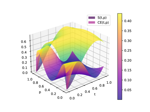
Figure 1: Plot for capacity of entanglement(CE ) and entanglement entropy (SEE ) vs p and t taking $\theta$ = 1

The plot in Fig.1 shows how entanglement entropy and capacity of entanglement varies for some chosen value of $\theta=1$, where capacity reduces to zero for when the state is either separable or stationary Shrimali et al. (2022); Dür et al. (2001).

Now, for evaluating bound on the rate of entanglement, we use the stronger-uncertainty relation in the form of Eqn. (12) for the two non-commuting operators $K_{AB}=K_{A}\otimes\mathcal{I}$ and $H_{AB}$. This leads to

$$\frac{1}{2}|\langle\Psi(t)|[K_{A}\otimes\mathcal{I},H_{AB}]|\Psi(t)\rangle|\leq\Delta K_{A}\hskip 2.84544pt\Delta H_{AB}\hskip 2.84544pt(1-R(t)).$$ (31)

Using Eqn. (14) (for $O=K_{A}$) in Eqn. (31), we then obtain

$$\frac{\hbar}{2}\left|\frac{{\rm d}\langle K_{A}\rangle}{{\rm d}t}\right|\leq\Delta K_{A}\hskip 2.84544pt\Delta H_{AB}\hskip 2.84544pt(1-R(t))\,.$$ (32)

Let $\Gamma(t)$ denote the rate of entanglement. Recall that the average of the modular Hamiltonian is the entanglement entropy $S_{EE}$. In terms of the entanglement rate $\Gamma(t)$, the above equation can be written as

$$\left|\Gamma(t)\right|\leq\frac{2}{\hbar}\Delta K_{A}\hskip 2.84544pt\Delta H_{AB}\hskip 2.84544pt(1-R(t))\,.$$ (33)

Since the square of the standard deviation of modular Hamiltonian is the capacity of entanglement, so in terms of the capacity of entanglement, we can write above bound as

$$\left|\Gamma(t)\right|\leq\frac{2}{\hbar}\sqrt{C_{E}(t)}\hskip 2.84544pt\Delta H_{AB}\hskip 2.84544pt(1-R(t))\,.$$ (34)

We can interpret the above formula by noting that one can define the speed of transportation of bipartite pure entangled state on projective Hilbert space of the given system by the expression $\frac{2}{\hbar}\Delta H_{AB}$. Further using the Fubini-Study metric for two nearby states, one can define the infinitesimal distance between two nearby states Anandan and Aharonov (1990); Pati (1991, 1995) as

$${\rm d}S^{2}=4\left(1-\left|\langle{\Psi(t)}\ket{\Psi(t+{\rm dt})}\right|^{2}\right)=\frac{4}{\hbar^{2}}\Delta H_{AB}^{2}\hskip 2.84544pt{\rm d}t^{2}.$$ (35)

Therefore, the speed of transportation as measured by the Fubini-Study metric is given by $V=\frac{{\rm d}S}{{\rm d}t}=\frac{2}{\hbar}\Delta H_{AB}$. Thus, the entanglement rate is upper bounded by the speed of quantum evolution Deffner and Campbell (2017b) and the square root of the capacity of entanglement and correction factor due to stronger uncertainty, i.e., $|\Gamma(t)|\leq\sqrt{C_{E}(t)}\hskip 2.84544ptV\hskip 2.84544pt(1-R(t))$.

We know from Ref. Bravyi (2007) that for an ancilla unassisted case, the entanglement rate is upper bounded by $c\|H\|\log d$, where $d={\rm min(dim}{\cal{H}}_{A},{\rm dim}{\cal{H}}_{B})$, $c$ being a constant between the value 1 and 2, and $\|H\|$ is operator norm of Hamiltonian which corresponds to $p=\infty$ of the Schatten p-norm of $H$ which is defined as $\|H\|_{p}=[\operatorname{tr}\left(\sqrt{H^{\dagger}H}\right)^{p}]^{\frac{1}{p}}$. Now, using the fact that the maximum value of capacity of entanglement is proportional to $S_{\rm max}(\rho_{A})^{2}$ de Boer et al. (2019b), where $S_{\rm{max}}(\rho_{A})$ is maximum value of von Neumann entropy of subsystem which is upper bounded by $\log{d}_{A}$, where $d_{A}$ is the dimension of Hilbert space of subsystem $A$, and $\Delta H\leq\|H\|$, a similar bound on the entanglement rate can be obtained from Eqn. (34). Further the factor $(1-R(t))$ varies between 0 and 1 for given standard choice of Eqn. (27). Thus, the bound on the entanglement rate given in Eqn. (34) is significantly stronger than the previously known bound and will be shown subsequently to be a improvement upon the bound found in Ref. Shrimali et al. (2022).

This bound on entanglement rate can be used to provide QSL which decides how fast a quantum state evolves in time from an initial state to a final state Pfeifer (1993). Even though it was discovered by Mandelstam and Tamm, over last one decade, there have been active explorations on generalising the notion of quantum speed limit for mixed states xiong Wu and shui Yu (2018); Mondal et al. (2016) and on resources that a quantum system might posses Campaioli et al. (2022). The notion of generalized quantum speed limit has been explored in Ref. Thakuria et al. (2022). Further, the quantum speed limit for observables has been defined and it was shown that the QSL for state evolution is a special case of the QSL for observable Mohan and Pati (2022). For a quantum system evolving under a given dynamics, there exists a fundamental limitation on the speed for entropy $S(\rho)$, maximal information $I(\rho)$, and quantum coherence $C(\rho)$ Mohan et al. (2022) as well as on other quantum correlations like entanglement, quantum mutual information and Bell-CHSH correlation Pandey et al. (2023).

Now, we are in the position to give a stronger uncertainty based expression for QSL bound,

$$\int_{0}^{T}\left|\frac{{\rm d}S_{EE}(t)}{{\rm d}t}\right|{{\rm d}t}\leq\int_{0}^{T}\frac{2}{\hbar}\sqrt{C_{E}(t)}\hskip 2.84544pt\Delta H\hskip 2.84544pt(1-R(t))\hskip 2.84544pt{\rm d}t.\\$$ (36)

For the time independent Hamiltonian, we obtain the following bound for the stronger quantum speed limit for entanglement

$$T\geq T_{\rm SQSLO}^{E}:=\frac{\hbar\left|S_{EE}(T)-S_{EE}(0)\right|}{2\Delta H\frac{1}{T}\int_{0}^{T}\sqrt{C_{E}(t)}\hskip 2.84544pt(1-R(t)){\rm d}t}.$$ (37)

It is thus clear that evolution speed for entanglement generation (or degradation) is a function of capacity of entanglement $C_{E}$ and a correction factor due to stronger uncertainty relation. Thus, we can say that $C_{E}$ with $(1-R(t))$ together controls how much time a system may take to produce certain amount of entanglement. Furthering our analysis of the bound, we have calculated $R(t)$ by using the above-prescribed expression. We note that under certain choice of $|\psi^{\perp}\rangle$ this corresponds to the system evolving along the geodesic path Thakuria and Pati (2022). The corresponding choice is as

$$|\psi^{\perp}(t)\rangle=\frac{O(t)-\langle O(t)\rangle}{\Delta O(t)}|\psi(t)\rangle,$$ (38)

and with this, the speed limit bound is the most optimized.

To examine the tightness of the given QSL bound for generation of entanglement by taking an example of the state as given in Eqn. (27) for which we have estimated both capacity of entanglement $C_{E}$ and entanglement entropy $S_{EE}$ in Eqn. (30). Further with $\Delta H=\hskip 1.42271pt\left|\theta\hskip 2.84544pt(1-2p)\right|$ and evaluating $R(t)$ as defined in Eqn. (13) making use of $\ket{\Psi^{\perp}(t)}$ through Eqn. (38) we plot for $T^{E}_{SQSLO}$ and $T^{E}_{QSLO}$ vs $T\in[0,1]$ in Fig. 2 where $T^{E}_{QSLO}$ is given as  Shrimali et al. (2022)

$$T\geq T_{\rm QSLO}^{E}:=\frac{\hbar\left|S_{EE}(T)-S_{EE}(0)\right|}{2\Delta H\frac{1}{T}\int_{0}^{T}\sqrt{C_{E}(t)}{\rm d}t}.$$ (39)

Figure 2: Here we depict $T_{QSLO}^{E},T_{SQSLO}^{E}$ vs T with p = 0.1 for $\theta$ = 1.0

We clearly see that the operator stronger quantum speed limit $T^{E}_{SQSLO}$ which is with the correction factor gives a significantly tighter bound than the other $T^{E}_{QSLO}$. With the choice of state and Hamiltonian with $p=0.1$ and $\theta=1.0$, we indeed show that the bound is tighter and achievable. Further, in Fig. 3, we plot $T^{E}_{SQSLO}$ vs $T$ for a fixed $p$ but several $\theta$ values, which shows that we get better bounds for lower values of $\theta$ and each of this case, $T^{E}_{SQSLO}$ gives a tighter bound.

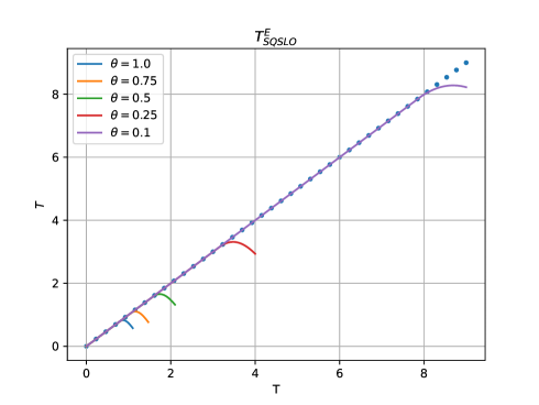
Figure 3: Speed limit plot for entanglement generation for varying $\theta$ keeping $p=0.1$ fixed.

In the subsequent section, we demonstrate that one obtains better bounds through SQSLO compared to QSLO by illustrating through two important examples.

V Illustrations and Examples

V.1 Improved Bounds on Modular energy using SQSLO

In the previous section, we have explored the study of entanglement generation using SQSL for state. Here, we would like to investigate how the modular Hamiltonian itself changes under unitary transformation in the Heisenberg picture. Consider a two-qubit system with a similar generalised canonical forms of non-local Hamiltonian $H^{\pm}$ as in Eqn. (24). Further our state in this case retains the form $\ket{\Psi}_{AB}=\ket{\Psi(0)}_{AB}$ as in Eqn. (26). As such the state operator of the composite system also retains its form as

$$\rho_{AB}=\rho_{AB}(0)=\ket{\Psi(0)}_{AB}\bra{\Psi(0)}.$$ (40)

We again choose $H^{+}$ form of canonical Hamiltonian to time evolve the following composite modular Hamiltonian

$$K_{AB}\equiv K_{AB}(0)=K_{A}\otimes\mathcal{I}_{B},$$ (41)

where $K_{A}\equiv K_{A}(0)=-\log{\rho_{A}}$ is the modular Hamiltonian and $\rho_{A}(0)=\operatorname{tr}_{B}(\rho_{AB}(0))$. In the Heisenberg picture, the operator of the composite $AB$ system evolves with unitary operator $U(t)=e^{-iH^{+}t}$

$$K_{AB}(t)=U^{\dagger}(t)K_{AB}(0)U(t).$$ (42)

We interpret the quantity $\langle K_{AB}(t)\rangle=\operatorname{tr}(\rho_{AB}\hskip 2.84544ptK_{AB}(t))$ as the modular energy $\mathcal{E_{M}}$ in the Heisenberg picture. Note that even though $\langle K_{AB}(0)\rangle=\operatorname{tr}(\rho_{A}(0)K_{A}(0))$ represents entanglement at $t=0$, $K_{AB}(t)$ does not represent entanglement at time $t$ in the Heisenberg picture.

Now, the variance of composite modular Hamiltonian $\mathcal{C_{M}}$ can be written as

$$\mathcal{C_{M}}(t)=\Delta K_{AB}(t)^{2}=\langle K_{AB}^{2}(t)\rangle-\langle K_{AB}(t)\rangle^{2}.$$ (43)

The generalised expression for the $\mathcal{E_{M}}$ and $\mathcal{C_{M}}$ can be evaluated and expressed as

$$\mathcal{C_{M}}(t)=\frac{1}{4} \log(-1+\frac{1}{p})^{2}\hskip 2.84544pt\left(4p(1-p)\hskip 2.84544pt\cos(2\theta)t)^{2}+\sin(2\theta t)^{2}\right)$$

$$\mathcal{E_{M}}(t)= -(1-2p)\hskip 2.84544pt\operatorname{arctanh}(1-2p)\hskip 2.84544pt\cos(2\theta t)$$

$$-\frac{1}{2}\log(p(1-p)).$$ (44)

We begin by making use of stronger-uncertainty relation for the case of in general non-commuting Hamiltonians $K_{AB}(t)$ and $H_{AB}$ and derive SQSLO bound for modular energy. Denoting $\ket{\Psi}_{AB}=\ket{\Psi}$ for brevity, we have

$$\frac{1}{2}|\langle\Psi|[K_{AB}(t),H_{AB}]|\Psi\rangle|\leq\Delta K_{AB}\Delta H_{AB}(1-R(t))$$ (45)

which leads to

$$\frac{\hbar}{2}\left|\frac{{\rm d}\langle K_{AB}(t)\rangle}{{\rm d}t}\right|=\frac{\hbar}{2}\left|\frac{{\rm d}\mathcal{E}_{M}}{{\rm d}t}\right|\leq\Delta K_{AB}(t)\Delta H_{AB}(1-R(t))\,.$$ (46)

As $\Delta K_{AB}(t)=\sqrt{\mathcal{C}_{M}(t)}$, from Eqn. (43), we get

$$\left|\frac{{\rm d}\mathcal{E}_{M}}{{\rm d}t}\right|\leq\frac{2}{\hbar}\sqrt{\mathcal{C}_{M}(t)}\Delta H_{AB}(1-R(t)).$$ (47)

This is a bound on the rate of the modular energy in the Heisenberg picture. This is clearly distinct from the earlier case in the Schrödinger picture (as these two quantities are different).

For the purpose of evaluating $R(t)$, we will need the optimized $\ket{\Psi^{\perp}}$ as prescribed in Eqn. (38). It is important to mention that though the state vector of the system $\ket{\Psi}$ remains time independent in the considered picture, yet $\ket{\Psi^{\perp}}$ carries an explicit time dependence due to the prescription used involving operators that are time evolving themselves. So at each instant of time of the operator evaluation, it picks up a different $\ket{\Psi^{\perp}}$ while only maintaining that it be perpendicular to the taken choice of $\ket{\Psi}$. It goes without saying that such $\ket{\Psi^{\perp}}$ is not physically relevant to the system, as it plays no role in the description of it at any point in time. The general expression for this choice evaluates out as given in Appendix A (67). Now this leads us to the following SQSLO bound as given by

$$T\geq T_{SQSLO}^{\mathcal{M}}:=\frac{\hbar}{2\hskip 2.84544pt\Delta H_{AB}}\int_{0}^{T}\frac{\left|{\rm d}\mathcal{E}_{M}\right|}{\sqrt{\mathcal{C}_{M}(t)}\hskip 2.84544pt\left(1-R(t)\right)}.$$ (48)

We get the equivalent $T^{\mathcal{M}}_{QSLO}$ case from the Robertson-Schrödinger uncertainty relation which is akin to dropping the correction factor from Eqn. (48)

$$T\geq T_{QSLO}^{\mathcal{M}}:=\frac{\hbar}{2\hskip 2.84544pt\Delta H_{AB}}\int_{0}^{T}\frac{\left|{\rm d}\mathcal{E}_{M}\right|}{\sqrt{\mathcal{C}_{M}(t)}\hskip 2.84544pt}.$$ (49)

Now, with $\Delta H_{AB}=\left|(1-2p)\hskip 2.84544pt\theta\right|$, we plot SQSLO and QSLO bounds in Fig. 4 for the case of $p=0.1$ and $\theta=1.0$ for which $R(t)$ is given in Eqn. (68).

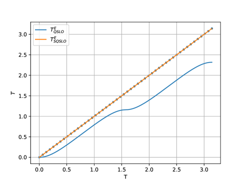
Figure 4: Here we depict $T_{QSLO}^{E},T_{SQSLO}^{E}$ vs T with p = 0.1 for $\theta$ = 1.0

We observe that in the case of Heisenberg picture, the QSLO bound, i.e., $T_{QSLO}^{\mathcal{M}}$ turns out to be a bit loose whereas the SQSLO bound, i.e., $T_{SQSLO}^{\mathcal{M}}$, which is with the correction factor turns out to be saturated.

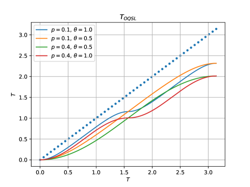
Figure 5: Depiction of $T_{QSLO}$ for chosen values of $p$ and $\theta$. The dotted line is the reference ideal case.

Finally, we plot for $T_{QSLO}^{\mathcal{M}}$ and $T_{SQSLO}^{\mathcal{M}}$ bounds for varying $\theta=0.5,1.0$ and fixed $p=0.1$ cases. We observe that the SQSLO bound turns out to be saturated for any choice in parameters. This shows that the SQSLO for the rate of modular Hamiltonian is tight and saturated.

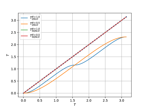
Figure 6: Depiction of $T_{QSLO}$ and $T_{SQSLO}$ for fixed $p$ and varying $\theta$.

V.2 Improved bounds on charging time of Quantum Batteries through SQSLO

The models of quantum engines and refrigerators have been of great interest lately as they help in simulating theoretical efforts to formulate fundamental thermodynamical principles and bounds which are valid on micro or nano-scale. It has been found that these can differ from the standard ones and converge only in the limit of macroscopic systems Alicki (1979). The amount of work that can be extracted from a small quantum mechanical system that is used to temporarily store energy and to transfer it from a production to a consumption center is the main content of a quantum battery. It is not coupled to external thermal baths in order to drive thermodynamical engines, but rather its dynamics is controlled by external time-dependent fields.

The battery comes with its initial state $\rho$ and an internal Hamiltonian $H_{B}$. The process of energy extraction then follows when this system is reversibly evolved under some fields that are turned on during time interval $[0,T]$. The maximal amount of work that can be extracted by such a process has been explored in Ref. Alicki and Fannes (2013) Subsequently, numerous researchers have dedicated their efforts to furthering the understanding and exploitation of non-classical features of quantum batteries such as in Ref. Kamin et al. (2020b). In many-body quantum systems characterized by multiple degrees of freedom, the presence of quantum batteries, capable of storing or releasing energy, is ubiquitous. In this section, we aim to determine the minimum achievable unitary charging time of the quantum battery utilizing the discussed SQSLO bound.

Consider a scenario where a quantum battery, with energy denoted by the Hamiltonian $H_{B}$, interacts with an external charging field represented by $H_{C}$. Consequently, the total energy of the system is determined by the combined Hamiltonian, expressed as follows:

$$H_{T}=H_{B}+H_{C}.$$ (50)

Now, the ergotropy is defined as the quantum system’s capacity to extract energy via unitary operations from the quantum battery Campaioli et al. (2018b), and is expressed as

$$\mathcal{E}(t)=\langle\Psi(t)|H_{B}|\Psi(t)\rangle-\langle\Psi(0)|H_{B}|\Psi(0)\rangle,$$ (51)

where $|\Psi(t)\rangle$ and $|\Psi(0)\rangle$ are the final and initial state of the given quantum system.

While the aforementioned expression holds true in the Schrödinger picture, we would now like to switch over to its study in the Heisenberg picture where the expression for ergotropy takes the form

$$\mathcal{E}(t)=\langle\Psi(0)|(H_{B}(t)-H_{B}(0))|\Psi(0)\rangle,$$ (52)

where $H_{B}(t)$ = $e^{\frac{iHt}{\hbar}}H_{B}(0)e^{-\frac{iHt}{\hbar}}$ and $H_{B}(0)$ = $H_{B}$.

The rate of change of ergotropy of quantum battery during the charging process can be obtained as

$$\frac{d\mathcal{E}(t)}{dt}=\frac{d}{dt}\langle\Psi(0)|H_{B}(t)|\Psi(0)\rangle.$$ (53)

Using our bound we can write SQSLO for the ergotropy as

$$T\geq\frac{\hbar}{2\Delta H_{T}}\int_{0}^{T}\frac{|d\mathcal{E}(t)|}{\Delta H_{B}(t)(1-R(t))},$$ (54)

where $R(t)$ = $\frac{1}{2}\left|\langle\Psi^{\perp}|\frac{H_{B}(t)}{\Delta H_{B}(t)}\mp i\frac{H_{T}}{\Delta H_{T}}|\Psi\rangle\right|^{2}$ and $T$ is the charging time period of the quantum battery.

This SQSLO for QBs can also be re-expressed as:

$$T_{SQSLO}^{QB}=\frac{\hbar T}{2\Delta H_{T}}\left<\left<\frac{\left|\mathcal{E}(T)-\mathcal{E}(0)\right|}{\Delta H_{B}(t)(1-R(t))}\right>\right>_{T},$$ (55)

where $\langle\langle A(t)\rangle\rangle_{T}$ = $\frac{1}{T}\int_{0}^{T}{\rm d}t\hskip 2.84544ptA(t)$, is the time average of the quantity $A(t)$.

Now that we have derived the Quantum speed limit (QSL) formula for Quantum Batteries (QB’s) in a general case, let us take up a specific example where we apply our SQSLO bound on QB’s. Our chosen example involves an entanglement-based QB consisting of two qubit cells and two coupled two-level systems. To charge the QB effectively, we must individually couple each cell with local fields. Consequently, our total Hamiltonian $H_{T}$ can be expressed as given in Ref. Kamin et al. (2020b)

$$H_{T}=H_{B}+H_{C}+H_{int},$$ (56)

where $H_{B}=\hbar\omega_{0}\sum_{n=1}^{2}\sigma_{n}^{z}$ being the battery Hamiltonian. Here, $\omega_{0}$ is the identical Larmor frequency for both the qubits. Let us label $\ket{\uparrow}$ and $\ket{\downarrow}$ as ground and excited states for a single qubit. With this one can define the fully charged state of the battery as $\ket{{\rm full}}=\ket{\uparrow\uparrow}$ with full energy $E_{{\rm full}}=2\hbar\omega$, and empty one as $\ket{{\rm emp}}=\ket{\downarrow\downarrow}$ with low energy $E_{{\rm emp}}=-2\hbar\omega$. Hence, the maximum energy that can be stored in the battery reads $\mathcal{E}_{{\rm max}}=4\hbar\omega$.

We consider the driving Hamiltonian to comprise of two parts, having charging part $H_{C}=\hbar\Omega\sum_{n=1}^{2}\sigma_{n}^{x}$ and nearest neighbour interaction part $H_{int}=\hbar J(\sigma_{1}^{x}\sigma_{2}^{x}+\sigma_{1}^{y}\sigma_{2}^{y}+\sigma_{1}^{z}\sigma_{2}^{z})$, where $J$ is the strength of two body interaction. The most general state of two qubits then reads as

$$\ket{\Psi(0)}=\mu\ket{\uparrow\uparrow}+\nu\ket{\uparrow\downarrow}+\eta\ket{\downarrow\uparrow}+\delta\ket{\downarrow\downarrow}.$$ (57)

Let us consider the case for the most general two qubit non-entangled state with,

$$\mu=\sin(\theta_{1})\sin(\theta_{2})e^{i(\varphi_{1}+\varphi_{2})}$$

$$\nu=\sin(\theta_{1})\cos(\theta_{2})e^{i\varphi_{1}}$$

$$\eta=\cos(\theta_{1})\sin(\theta_{2})e^{i\varphi_{2}}$$

$$\delta=\cos(\theta_{1})\cos(\theta_{2})$$ (58)

where $\theta_{1},\theta_{2}\in[0,\pi]$ and $\varphi_{1},\varphi_{2}\in[0,2\pi]$. For the purpose of illustration, let us assume that at the beginning of the charging process, the battery is assumed to be empty, i.e., $\rho(0)=\ket{{\rm emp}}\bra{{\rm emp}}$, which is achieved when we put $\theta_{1}=\theta_{2}=0$ in Eqn. (58).

The ergotropy Eqn. (52) in this case under Heisenberg picture upon evaluation reads as

$$\mathcal{E}(t)=\frac{4\omega\Omega^{2}}{\omega^{2}+\Omega^{2}}\sin\left(\sqrt{\omega^{2}+\Omega^{2}}\hskip 2.84544ptt\right)^{2}.$$ (59)

Utilizing the expression of QSLO, we arrive at our SQSLO bound, which reads as

$$T_{QSLO}=\frac{\hbar}{2\Delta H_{T}}\int_{0}^{T}\frac{|d\mathcal{E}(t)|}{\Delta H_{B}(t)},$$ (60)

where $\Delta H_{T}$ and $\Delta H_{B}(t)$ can be evaluated for chosen values of parameters $\omega$, $\Omega$ and $J$ in above bound.

With our general Hamiltonian for QB defined as above, let us take a case of parallel charging when $J=0$, rendering the interaction Hamiltonian inactive. Similarly, we can determine the QSLO for the case of collective charging when $J\neq 0$ using Eqn. (60). Upon plotting these two-speed limit functions, as depicted in Fig. 7, we observe that for the above two cases, the QSLO bound overlaps. Over that, there is a clear deviation from the reference ideal case, i.e., $T_{QSLO}=T$. It thus leaves the ground for improvement. This observation holds true for both scenarios of the QB Hamiltonian, namely the parallel and collective charging cases. Hence, we would like to compute the bounds by applying the SQSLO bound to both the cases.

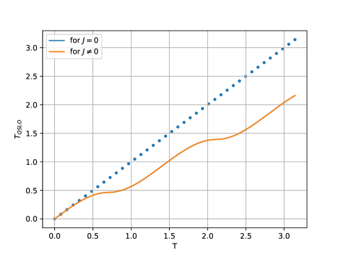
Figure 7: This plot shows that the QSLO bound plot for both parallel and collective QB scenarios, where $J=0$ and $J\neq 0$ respectively with respect to reference line.

Next, we study the scenarios involving coupled and decoupled cases. When $J=\Omega$, we say the system is coupled, whereas for $J\neq\Omega$, it represents the decoupled scenario. To compute the QSLO for both the coupled and decoupled Hamiltonians, we follow a similar procedure as we did for the parallel and collective QB cases. A novel aspect of our approach is the application of the SQSLO in both the coupled and decoupled Hamiltonians. The expression for the SQSLO bound is given as

$$T_{SQSLO}=\frac{\hbar}{2\Delta H_{T}}\int_{0}^{T}\frac{\left|d\mathcal{E}(t)\right|}{\Delta H_{B}(t)(1-R(t))},$$ (61)

where for the coupled case (with $J=\Omega=1$ and $\omega=2$) we obtain expression of $R(t)$ as

$$R(t)=\frac{1}{2}\left(\begin{cases}2-\frac{2\sqrt{10}\cos(\sqrt{5}t)}{\sqrt{9+\cos(2\sqrt{5}t)}}&\sin(\sqrt{5}t)<0\\ 2+\frac{2\sqrt{10}\cos(\sqrt{5}t)}{\sqrt{9+\cos(2\sqrt{5}t)}}&\text{True},\end{cases}\right),$$ (62)

where $|\Psi\rangle$ and $|\Psi^{\perp}\rangle$ are given in Appendix-B. For the purpose of evaluating $R(t)$, we need the optimized $\ket{\Psi^{\perp}}$ as prescribed in Eqn. (38).

Again, for the decoupled case, i.e., $J\neq\Omega$ (taking $J=1,\hskip 2.84544pt\Omega=4,\hskip 2.84544pt\omega=2$) we evaluate the bound using the expression for bound in Eqn. (61). The expression of $R(t)$ upon evaluation comes as

$$R(t)=\frac{1}{2}\left(\begin{cases}2-\frac{4\cos(2\sqrt{2}t)}{\sqrt{3+\cos(4\sqrt{2}t)}}&\sin(2\sqrt{2}t)<0\\ 2+\frac{4\cos(2\sqrt{2}t)}{\sqrt{3+\cos(4\sqrt{2}t)}}&\text{True},\end{cases}\right),$$ (63)

where $|\Psi\rangle$ and $|\Psi^{\perp}\rangle$ are given in Appendix-B.

We have depicted both SQSLO curves for both the coupling and decoupling cases. Surprisingly, in both scenarios, the SQSLO plots exhibit remarkable accuracy as they overlap while showing saturation, as can be seen in Fig. 8. As expected, QSLO does not yield optimally tight bounds for both coupling and decoupling cases as shown in the same figure. From these plots, we can conclude that SQSLO performs remarkably well, accurately representing the speed limit behavior in QB systems for both coupling and decoupling cases. This result is quite a significant improvement upon earlier bounds and is the optimal bound. Next, we will apply SQSLO in parallel and collective QB cases to further explore its behavior in those scenarios.

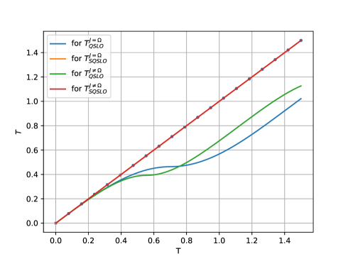
Figure 8: This plot shows that the QSLO and SQSLO bound plot for both coupling and decoupling QB scenarios, where $J=\Omega$ and $J\neq\Omega$ respectively.

Having computed the QSLO for both parallel ($J=0$) and collective charging ($J\neq 0$) QB cases, we will now apply the SQSLO bound in both these cases. This involves evaluation of $R(t)$ for both scenarios. We have already given the expression for collective charging ($J\neq 0$) case earlier. For parallel charging ($J=0$) case with $\Omega=1,\hskip 2.84544pt\omega=2$; this reads as

$$R(t)=\frac{1}{2}\left(2+\frac{2\sqrt{10}\hskip 2.84544pt\left|\sin(\sqrt{5}t)\right|\cot(\sqrt{5}t)}{\sqrt{9+\cos(2\sqrt{5}t)}}\right),$$ (64)

where the involved $|\Psi\rangle$ and $|\Psi^{\perp}\rangle$ in this case are given in Appendix-B.

From the previous expressions, we reiterate that it appears that $|\Psi^{\perp}\rangle$ exhibits time dependence. However, according to the Heisenberg picture, the state should not evolve, indicating that we should not observe time dependence in the orthogonal state. Fundamentally, we acknowledge the existence of multiple choices for the orthogonal state of a given state. Therefore, we have adopted the most widely accepted method to select the orthogonal state to optimize our parameter $R$. In Eqn. (38) , we notice that the observable $O$ is involved in the formula, and we employ its associated battery Hamiltonian $H_{B}(t)$, which evolves in the Heisenberg picture. Consequently, the time dependence on $|\Psi^{\perp}\rangle$ state arises. Through this selection, we achieve optimal value for the expression $R$.

Now, it is interesting to observe the behavior of SQSLO over a longer duration. We have plotted SQSLO for an extended period of time, and we observe optimal results, as illustrated in Fig. 9. Thus, one can affirm that for QB scenarios, SQSLO stands as the optimal choice—it represents the best bound for calculating the charging time of quantum batteries.

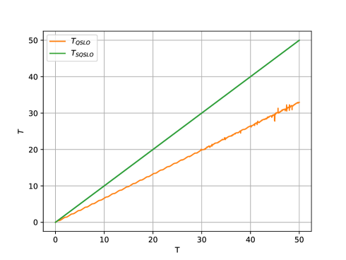
Figure 9: Here we depict $T_{QSLO},T_{SQSLO}$ vs T for long time

We have analysed various quantum battery scenarios, including parallel, collective, coupling and decoupling cases, and presented our findings for QSLO and SQSLO. It is evident that SQSLO consistently reveals the tightest bound for quantum speed limit. Consequently, we can assert that SQSLO outperforms in predicting the charging time.

VI Conclusion

In conclusion, we have addressed the fundamental question of how fast an observable can evolve in time by invoking the concept of the observable speed limit. Our study presents a stronger version of this limit, demonstrating that previously derived bounds are special cases of our new bound. We have also shown that SQSLO can lead to stronger speed limit for states. By applying SQSLO, we have investigated its efficacy in evaluating the capacity of entanglement, akin to the heat capacity in quantum information theory. Notably, we have established a more robust bound for the entanglement rate, surpassing previous limitations. Moreover, our exploration extends to the realm of interacting qubits within quantum batteries. By leveraging SQSLO, we have accurately predicted the time required to charge the battery, showcasing the tightness of SQSLO in this context—it effectively saturates when estimating the charging time of quantum batteries. These findings hold significant implications across various domains, including quantum thermodynamics, the complexity of operator growth, prediction of quantum correlation growth rates, and the broader landscape of quantum technology. Thus, SQSLO emerges as a powerful tool with diverse applications, paving the way for advancements in quantum science and technology.

Acknowledgments: DS acknowledges the support of the INFOSYS scholarship. BP acknowledges IIIT, Hyderabad and TCG CREST (CQuERE) for their support and hospitality during the academic visit.

Appendix A SQSL bound for Entanglement Capacity

SQSL bound for entanglement generation using the capacity of entanglement under Schrödinger picture requires the functional form of $R(t)$ and $\ket{\Psi^{\perp}}$ as defined in Eq.(38)

$$R(t)=\frac{\left|\sqrt{-\operatorname{arctanh}(\alpha)^{2}\beta}/\sqrt{2}+\operatorname{arctanh}(\alpha)\hskip 2.84544pt{\rm Sign}((1-2p)\theta)\hskip 2.84544pt(-2i\sqrt{p(1-p)}\hskip 2.84544pt\cos(2\theta t)-\sin(2\theta t))\right|^{2}}{\left|\operatorname{arctanh}(\alpha)^{2}\hskip 2.84544pt\beta\right|},$$ (65)

where $\alpha=(2p-1)\cos(2\theta t)$, $\beta=-1-4p(1-p)+(1-2p)^{2}\cos(4\theta t)$. Also,

$$|\Psi^{\perp}\rangle=\left(\begin{array}[]{c}\frac{{\sqrt{2}e^{-it\mu_{3}}\operatorname{arctan}\left[(-1+2p)\cos\left(2t\theta\right)\right]\left(-1+(-1+2p)\cos\left(2t\theta\right)\right)\left(\sqrt{p}\cos\left(t\theta\right)-i\sqrt{1-p}\sin\left(t\theta\right)\right)}}{{\sqrt{-\operatorname{arctanh}\left[(-1+2p)\cos\left(2t\theta\right)\right]^{2}\left(-1+4(-1+p)p+(1-2p)^{2}\cos\left(4t\theta\right)\right)}}}\\ 0\\ 0\\ \frac{{\sqrt{2}e^{-it\mu_{3}}\operatorname{arctanh}\left[(-1+2p)\cos\left(2t\theta\right)\right]\left(1+(-1+2p)\cos\left(2t\theta\right)\right)\left(\sqrt{1-p}\cos\left(t\theta\right)-i\sqrt{p}\sin\left(t\theta\right)\right)}}{{\sqrt{-\operatorname{arctanh}\left[(-1+2p)\cos\left(2t\theta\right)\right]^{2}\left(-1+4(-1+p)p+(1-2p)^{2}\cos\left(4t\theta\right)\right)}}}\end{array}\right),$$ (66)

where $\theta=(\mu_{1}-\mu_{2})$.

Similarly, SQSLO bound for generation of modular energy using the composite modular Hamiltonian under the Heisenberg picture requires the functional form of $R(t)$ and $\ket{\Psi^{\perp}}$ as defined in Eq.(38).

$$|\Psi^{\perp}\rangle=\left(\begin{array}[]{c}\frac{\log{\left(-1+\frac{1}{p}\right)}\left(-2\left(-1+p\right)\sqrt{p}\cos{\left(2\hskip 1.42271pt\theta\hskip 1.42271ptt\right)}-i\sqrt{1-p}\sin{\left(2\hskip 1.42271pt\theta\hskip 1.42271ptt\right)}\right)}{\sqrt{\log^{2}{\left(-1+\frac{1}{p}\right)}\left(-4\left(-1+p\right)p\cos^{2}{\left(2\hskip 1.42271pt\theta\hskip 1.42271ptt\right)}+\sin^{2}{\left(2\hskip 1.42271pt\theta\hskip 1.42271ptt\right)}\right)}}\\ 0\\ 0\\ \frac{\log{\left(-1+\frac{1}{p}\right)}\left(-2\sqrt{\left(1-p\right)p}\cos{\left(2\hskip 1.42271pt\theta\hskip 1.42271ptt\right)}+i\sin{\left(2\hskip 1.42271pt\theta\hskip 1.42271ptt\right)}\right)}{\sqrt{\frac{\log^{2}{\left(-1+\frac{1}{p}\right)}\left(-4\left(-1+p\right)p\cos^{2}{\left(2\hskip 1.42271pt\theta\hskip 1.42271ptt\right)}+\sin^{2}{\left(2\hskip 1.42271pt\theta\hskip 1.42271ptt\right)}\right)}{p}}}\\ \end{array}\right),$$ (67)

For $p$ = $0.1$ and $\Theta$ = $1$, $R$ is given as:

$$R(t)=\frac{0.63\left|1.89+\cos(2t)\left(1.67i\sqrt{0.68-0.32\cos(4t)}\right)-0.89\cos(4t)+2.78\sqrt{0.68-0.32\cos(4t)}\sin(2t)\right|^{2}}{(2.13-\cos(4t))^{2}},$$ (68)

Again, for $p$ = $0.1$ and $\Theta$ = $0.5$, $R$ is given as:

$$R(t)=-\frac{{0.15\left|\cos(t)^{2}+\cos(t)\left(1.67i)\sqrt{0.68-0.32\cos(2t)}\right)+\sin(t)\left(2.78\sqrt{0.68-0.32\cos(2t)}+2.78\sin(t)\right)\right|^{2}}}{-1.18+\cos(2t)-0.12\cos(4t)},$$ (69)

Again, for $p$ = $0.4$ and $\Theta$ = $1$, $R$ is given as:

$$R(t)=0.5\left|\frac{1}{(-49+\cos(4t))}\left(-49+\cos(4t)-(48.99i)\sqrt{0.98-0.02\cos(4t)}\left(\cos(2t)-(2.04i)\cos(t)\sin(t)\right)\right)\right|^{2},$$ (70)

At last, for $p$ = $0.4$ and $\Theta$ = $0.5$, $R$ is given as:

$$R(t)=-\frac{{11.76\left|\cos(t)^{2}+\cos(t)\left(-1.02i\sqrt{0.98-0.02\cos(2t)}\right)+\sin(t)\left(1.04\sqrt{0.98-0.02\cos(2t)}+1.04\sin(t)\right)\right|^{2}}}{{-24.51+\cos(2t)-0.005\cos(4t)}}.$$ (71)

Appendix B Related to Quantum Battery

There are three cases in which we have calculated the SQSLO for QBs. For each case, we require the values of $|\Psi\rangle$, and $|\Psi^{\perp}\rangle$. We will define each of these components individually.

Here, for all cases the initial state is:

$$|\Psi\rangle=(0,0,0,1)^{T},$$ (72)

For $J=1$, $\omega=2$ and $\Omega=1$, the function $R(t)$ in Eq. (62), $|\Psi^{\perp}\rangle$ is provided below:

$$|\Psi^{\perp}\rangle=\left(\begin{array}[]{c}0\\ \frac{2-2\cos(2\sqrt{5}t)-i\sqrt{5}\sin(2\sqrt{5}t)}{2\left|\sin(\sqrt{5}t)\right|\sqrt{9+\cos(2\sqrt{5}t)}}\\ \frac{2-2\cos(2\sqrt{5}t)-i\sqrt{5}\sin(2\sqrt{5}t)}{2\left|\sin(\sqrt{5}t)\right|\sqrt{9+\cos(2\sqrt{5}t)}}\\ 0\end{array}\right).$$ (73)

For $J=1$, $\omega=2$ and $\Omega=4$, the function $R(t)$ in Eq. (63), $\Psi^{\perp}\rangle$ is provided below:

$$|\Psi^{\perp}\rangle=\left(\begin{array}[]{c}0\\ \frac{1-\cos(4\sqrt{5}t)-t\sqrt{5}\sin(4\sqrt{5}t)}{2\left|\sin(2\sqrt{5}t)\right|\sqrt{6+4\cos(4\sqrt{5}t)}}\\ \frac{1-\cos(4\sqrt{5}t)-t=\sqrt{5}\sin(4\sqrt{5}t)}{2\left|\sin(2\sqrt{5}t)\right|\sqrt{6+4\cos(4\sqrt{5}t)}}\\ 0\end{array}\right).$$ (74)

For $J=0$, $\omega=2$ and $\Omega=1$, the functions $R(t)$ in Eq. (64), $|\Psi^{\perp}\rangle$ is provided below:

$$|\Psi^{\perp}\rangle=\left(\begin{array}[]{c}0\\ \frac{e^{-2i+\sqrt{5}t}(-2+\sqrt{5}+4e^{2i+\sqrt{5}t}-(2+\sqrt{5})e^{4i\sqrt{5}t})}{4\left|\sin(\sqrt{5}\hskip 2.84544ptt)\right|\sqrt{9+\cos(2\sqrt{5}t)}}\\ \frac{e^{-2i+\sqrt{5}t}(-2+\sqrt{5}+4e^{2i+\sqrt{5}t}-(2+\sqrt{5})e^{4+\sqrt{5}}t)}{4\left|\sin(\sqrt{5}\hskip 2.84544ptt)\right|\sqrt{9+\cos(2\sqrt{5}t)}}\\ 0\end{array}\right).$$ (75)

References

- Mandelstam and Tamm (1945) Leonid Mandelstam and IG Tamm, “The uncertainty relation between energy and time in non-relativistic quantum mechanics,” J. Phys. (USSR) 9, 249 (1945).
- Anandan and Aharonov (1990) Jeeva Anandan and Yakir Aharonov, “Geometry of quantum evolution,” Phys. Rev. Lett. 65, 1697–1700 (1990).
- Pati (1991) Arun Kumar Pati, “Relation between “phases” and “distance” in quantum evolution,” Physics Letters A 159, 105–112 (1991).
- Margolus and Levitin (1998) Norman Margolus and Lev B. Levitin, “The maximum speed of dynamical evolution,” Physica D: Nonlinear Phenomena 120, 188–195 (1998).
- Levitin and Toffoli (2009) Lev B. Levitin and Tommaso Toffoli, “Fundamental limit on the rate of quantum dynamics: The unified bound is tight,” Phys. Rev. Lett. 103, 160502 (2009).
- Gislason et al. (1985) Eric A. Gislason, Nora H. Sabelli, and John W. Wood, “New form of the time-energy uncertainty relation,” Phys. Rev. A 31, 2078–2081 (1985).
- Eberly and Singh (1973) Joseph H. Eberly and L. P. S. Singh, “Time operators, partial stationarity, and the energy-time uncertainty relation,” Phys. Rev. D 7, 359–362 (1973).
- Bauer and Mello (1978) M Bauer and P.A Mello, “The time-energy uncertainty relation,” Annals of Physics 111, 38–60 (1978).
- Bhattacharyya (1983) K Bhattacharyya, “Quantum decay and the mandelstam-tamm-energy inequality,” Journal of Physics A: Mathematical and General 16, 2993 (1983).
- Leubner and Kiener (1985) C. Leubner and C. Kiener, “Improvement of the eberly-singh time-energy inequality by combination with the mandelstam-tamm approach,” Phys. Rev. A 31, 483–485 (1985).
- Vaidman (1992) Lev Vaidman, “Minimum time for the evolution to an orthogonal quantum state,” American Journal of Physics 60, 182–183 (1992), https://pubs.aip.org/aapt/ajp/article-pdf/60/2/182/12124296/182_1_online.pdf .
- Uhlmann (1992) Armin Uhlmann, “An energy dispersion estimate,” Physics Letters A 161, 329–331 (1992).
- Uffink (1993) Jozef B Uffink, “The rate of evolution of a quantum state,” American Journal of Physics 61, 935–936 (1993).
- Pfeifer and Fröhlich (1995) Peter Pfeifer and Jürg Fröhlich, “Generalized time-energy uncertainty relations and bounds on lifetimes of resonances,” Rev. Mod. Phys. 67, 759–779 (1995).
- Horesh and Mann (1998) N Horesh and A Mann, “Intelligent states for the anandan - aharonov parameter-based uncertainty relation,” Journal of Physics A: Mathematical and General 31, L609 (1998).
- Pati (1999) Arun Kumar Pati, “Uncertainty relation of anandan–aharonov and intelligent states,” Physics Letters A 262, 296–301 (1999).
- Söderholm et al. (1999) Jonas Söderholm, Gunnar Björk, Tedros Tsegaye, and Alexei Trifonov, “States that minimize the evolution time to become an orthogonal state,” Phys. Rev. A 59, 1788–1790 (1999).
- Andrecut and Ali (2004) M Andrecut and M K Ali, “The adiabatic analogue of the margolus–levitin theorem,” Journal of Physics A: Mathematical and General 37, L157 (2004).
- Gray and Vogt (2005) John Gray and Andrew Vogt, “Mathematical analysis of the mandelstam-tamm time-energy uncertainty principle,” Journal of Mathematical Physics 46 (2005), 10.1063/1.1897164.
- Zieliński and Zych (2006) Bartosz Zieliński and Magdalena Zych, “Generalization of the margolus-levitin bound,” Phys. Rev. A 74, 034301 (2006).
- Andrews (2007) Mark Andrews, “Bounds to unitary evolution,” Phys. Rev. A 75, 062112 (2007).
- Yurtsever (2010) Ulvi Yurtsever, “Fundamental limits on the speed of evolution of quantum states,” Physica Scripta 82, 035008 (2010).
- Shuang-Shuang et al. (2010) Fu Shuang-Shuang, Li Nan, and Luo Shun-Long, “A note on fundamental limit of quantum dynamics rate,” Communications in Theoretical Physics 54, 661 (2010).
- Poggi et al. (2013) P. M. Poggi, F. C. Lombardo, and D. A. Wisniacki, “Quantum speed limit and optimal evolution time in a two-level system,” Europhysics Letters 104, 40005 (2013).
- Kupferman and Reznik (2008) Judy Kupferman and Benni Reznik, “Entanglement and the speed of evolution in mixed states,” Phys. Rev. A 78, 042305 (2008).
- Jones and Kok (2010) Philip J. Jones and Pieter Kok, “Geometric derivation of the quantum speed limit,” Phys. Rev. A 82, 022107 (2010).
- Chau (2010) H. F. Chau, “Tight upper bound of the maximum speed of evolution of a quantum state,” Phys. Rev. A 81, 062133 (2010).
- Deffner and Lutz (2013) Sebastian Deffner and Eric Lutz, “Energy–time uncertainty relation for driven quantum systems,” Journal of Physics A: Mathematical and Theoretical 46, 335302 (2013).
- Fung and Chau (2014) Chi-Hang Fred Fung and H. F. Chau, “Relation between physical time-energy cost of a quantum process and its information fidelity,” Phys. Rev. A 90, 022333 (2014).
- Andersson and Heydari (2014) O Andersson and H Heydari, “Quantum speed limits and optimal hamiltonians for driven systems in mixed states,” Journal of Physics A: Mathematical and Theoretical 47, 215301 (2014).
- Mondal et al. (2016) Debasis Mondal, Chandan Datta, and Sk Sazim, “Quantum coherence sets the quantum speed limit for mixed states,” Physics Letters A 380, 689–695 (2016).
- Mondal and Pati (2016) Debasis Mondal and Arun Kumar Pati, “Quantum speed limit for mixed states using an experimentally realizable metric,” Physics Letters A 380, 1395–1400 (2016).
- Deffner and Campbell (2017a) Sebastian Deffner and Steve Campbell, “Quantum speed limits: from heisenberg’s uncertainty principle to optimal quantum control,” Journal of Physics A: Mathematical and Theoretical 50, 453001 (2017a).
- Campaioli et al. (2018a) Francesco Campaioli, Felix A. Pollock, Felix C. Binder, and Kavan Modi, “Tightening quantum speed limits for almost all states,” Phys. Rev. Lett. 120, 060409 (2018a).
- Ashhab et al. (2012) S. Ashhab, P. C. de Groot, and Franco Nori, “Speed limits for quantum gates in multiqubit systems,” Phys. Rev. A 85, 052327 (2012).
- Mukhopadhyay et al. (2018) Chiranjib Mukhopadhyay, Avijit Misra, Samyadeb Bhattacharya, and Arun Kumar Pati, “Quantum speed limit constraints on a nanoscale autonomous refrigerator,” Phys. Rev. E 97, 062116 (2018).
- Funo et al. (2019) Ken Funo, Naoto Shiraishi, and Keiji Saito, “Speed limit for open quantum systems,” New Journal of Physics 21, 013006 (2019).
- Caneva et al. (2009) T. Caneva, M. Murphy, T. Calarco, R. Fazio, S. Montangero, V. Giovannetti, and G. E. Santoro, “Optimal control at the quantum speed limit,” Physical Review Letters 103 (2009), 10.1103/physrevlett.103.240501.
- Campbell and Deffner (2017) Steve Campbell and Sebastian Deffner, “Trade-off between speed and cost in shortcuts to adiabaticity,” Physical Review Letters 118 (2017), 10.1103/physrevlett.118.100601.
- Campbell et al. (2018) Steve Campbell, Marco G Genoni, and Sebastian Deffner, “Precision thermometry and the quantum speed limit,” Quantum Science and Technology 3, 025002 (2018).
- Maccone and Pati (2014) Lorenzo Maccone and Arun K. Pati, “Stronger uncertainty relations for all incompatible observables,” Phys. Rev. Lett. 113, 260401 (2014).
- Thakuria and Pati (2022) Dimpi Thakuria and Arun Kumar Pati, “Stronger quantum speed limit,” (2022), arXiv:2208.05469 [quant-ph] .
- Mohan and Pati (2022) Brij Mohan and Arun Kumar Pati, “Quantum speed limits for observables,” Phys. Rev. A 106, 042436 (2022).
- Horodecki et al. (2009) Ryszard Horodecki, Paweł Horodecki, Michał Horodecki, and Karol Horodecki, “Quantum entanglement,” Reviews of Modern Physics 81, 865 (2009).
- Das et al. (2016) Sreetama Das, Titas Chanda, Maciej Lewenstein, Anna Sanpera, Aditi Sen De, and Ujjwal Sen, “The separability versus entanglement problem,” Quantum Information: From Foundations to Quantum Technology Applications , 127 (2016).
- de Boer et al. (2019a) Jan de Boer, Jarkko Järvelä, and Esko Keski-Vakkuri, “Aspects of capacity of entanglement,” Physical Review D 99, 066012 (2019a).
- Shrimali et al. (2022) Divyansh Shrimali, Swapnil Bhowmick, Vivek Pandey, and Arun Kumar Pati, “Capacity of entanglement for a nonlocal hamiltonian,” Phys. Rev. A 106, 042419 (2022).
- de Boer et al. (2019b) Jan de Boer, Jarkko Järvelä, and Esko Keski-Vakkuri, “Aspects of capacity of entanglement,” Physical Review D 99, 066012 (2019b).
- Laflorencie (2016) Nicolas Laflorencie, “Quantum entanglement in condensed matter systems,” Physics Reports 646, 1 (2016).
- Yao and Qi (2010) Hong Yao and Xiao-Liang Qi, “Entanglement entropy and entanglement spectrum of the kitaev model,” Physical Review Letters 105, 080501 (2010).
- Alicki and Fannes (2013) Robert Alicki and Mark Fannes, “Entanglement boost for extractable work from ensembles of quantum batteries,” Phys. Rev. E 87, 042123 (2013).
- Binder et al. (2015) Felix C Binder, Sai Vinjanampathy, Kavan Modi, and John Goold, “Quantacell: powerful charging of quantum batteries,” New Journal of Physics 17, 075015 (2015).
- Campaioli et al. (2017) Francesco Campaioli, Felix A. Pollock, Felix C. Binder, Lucas Céleri, John Goold, Sai Vinjanampathy, and Kavan Modi, “Enhancing the charging power of quantum batteries,” Phys. Rev. Lett. 118, 150601 (2017).
- Rossini et al. (2020) Davide Rossini, Gian Marcello Andolina, Dario Rosa, Matteo Carrega, and Marco Polini, “Quantum advantage in the charging process of sachdev-ye-kitaev batteries,” Phys. Rev. Lett. 125, 236402 (2020).
- Gyhm et al. (2022) Ju-Yeon Gyhm, Dominik Šafránek, and Dario Rosa, “Quantum charging advantage cannot be extensive without global operations,” Phys. Rev. Lett. 128, 140501 (2022).
- Gyhm and Fischer (2024) Ju-Yeon Gyhm and Uwe R. Fischer, “Beneficial and detrimental entanglement for quantum battery charging,” AVS Quantum Science 6 (2024), 10.1116/5.0184903.
- Julià-Farré et al. (2020) Sergi Julià-Farré, Tymoteusz Salamon, Arnau Riera, Manabendra N. Bera, and Maciej Lewenstein, “Bounds on the capacity and power of quantum batteries,” Phys. Rev. Res. 2, 023113 (2020).
- Campaioli et al. (2023) Francesco Campaioli, Stefano Gherardini, James Q. Quach, Marco Polini, and Gian Marcello Andolina, “Colloquium: Quantum batteries,” (2023), arXiv:2308.02277 [quant-ph] .
- Andolina et al. (2018) Gian Marcello Andolina, Donato Farina, Andrea Mari, Vittorio Pellegrini, Vittorio Giovannetti, and Marco Polini, “Charger-mediated energy transfer in exactly solvable models for quantum batteries,” Phys. Rev. B 98, 205423 (2018).
- Le et al. (2018) Thao P. Le, Jesper Levinsen, Kavan Modi, Meera M. Parish, and Felix A. Pollock, “Spin-chain model of a many-body quantum battery,” Phys. Rev. A 97, 022106 (2018).
- Zhang et al. (2019) Yu-Yu Zhang, Tian-Ran Yang, Libin Fu, and Xiaoguang Wang, “Powerful harmonic charging in a quantum battery,” Phys. Rev. E 99, 052106 (2019).
- Barra (2019) Felipe Barra, “Dissipative charging of a quantum battery,” Phys. Rev. Lett. 122, 210601 (2019).
- Santos et al. (2019) Alan C. Santos, Barı ş Çakmak, Steve Campbell, and Nikolaj T. Zinner, “Stable adiabatic quantum batteries,” Phys. Rev. E 100, 032107 (2019).
- Andolina et al. (2019) Gian Marcello Andolina, Maximilian Keck, Andrea Mari, Michele Campisi, Vittorio Giovannetti, and Marco Polini, “Extractable work, the role of correlations, and asymptotic freedom in quantum batteries,” Phys. Rev. Lett. 122, 047702 (2019).
- Crescente et al. (2020a) Alba Crescente, Matteo Carrega, Maura Sassetti, and Dario Ferraro, “Ultrafast charging in a two-photon dicke quantum battery,” Phys. Rev. B 102, 245407 (2020a).
- Santos et al. (2020) Alan C. Santos, Andreia Saguia, and Marcelo S. Sarandy, “Stable and charge-switchable quantum batteries,” Phys. Rev. E 101, 062114 (2020).
- Santos (2021) Alan C. Santos, “Quantum advantage of two-level batteries in the self-discharging process,” Phys. Rev. E 103, 042118 (2021).
- Dou et al. (2022) Fu-Quan Dou, You-Qi Lu, Yuan-Jin Wang, and Jian-An Sun, “Extended dicke quantum battery with interatomic interactions and driving field,” Phys. Rev. B 105, 115405 (2022).
- Barra et al. (2022) Felipe Barra, Karen V Hovhannisyan, and Alberto Imparato, “Quantum batteries at the verge of a phase transition,” New Journal of Physics 24, 015003 (2022).
- Carrasco et al. (2022) Javier Carrasco, Jerónimo R. Maze, Carla Hermann-Avigliano, and Felipe Barra, “Collective enhancement in dissipative quantum batteries,” Phys. Rev. E 105, 064119 (2022).
- Shaghaghi et al. (2022) Vahid Shaghaghi, Varinder Singh, Giuliano Benenti, and Dario Rosa, “Micromasers as quantum batteries,” Quantum Science and Technology 7, 04LT01 (2022).
- Rodríguez et al. (2023) Carla Rodríguez, Dario Rosa, and Jan Olle, “Artificial intelligence discovery of a charging protocol in a micromaser quantum battery,” Phys. Rev. A 108, 042618 (2023).
- Santos et al. (2023) Tiago F. F. Santos, Yohan Vianna de Almeida, and Marcelo F. Santos, “Vacuum-enhanced charging of a quantum battery,” Phys. Rev. A 107, 032203 (2023).
- Kamin et al. (2023) F H Kamin, Z Abuali, H Ness, and S Salimi, “Quantum battery charging by non-equilibrium steady-state currents,” Journal of Physics A: Mathematical and Theoretical 56, 275302 (2023).
- Downing and Ukhtary (2023) Charles Andrew Downing and Muhammad Shoufie Ukhtary, “A quantum battery with quadratic driving,” Communications Physics 6 (2023), 10.1038/s42005-023-01439-y.
- Hadipour et al. (2023) Maryam Hadipour, Soroush Haseli, Dong Wang, and Saeed Haddadi, “Practical scheme for realization of a quantum battery,” (2023), arXiv:2312.06389 [quant-ph] .
- Kamin et al. (2020a) F. H. Kamin, F. T. Tabesh, S. Salimi, and Alan C. Santos, “Entanglement, coherence, and charging process of quantum batteries,” Phys. Rev. E 102, 052109 (2020a).
- Pirmoradian and Mølmer (2019) Faezeh Pirmoradian and Klaus Mølmer, “Aging of a quantum battery,” Phys. Rev. A 100, 043833 (2019).
- Zhang and Blaauboer (2023) Xiang Zhang and Miriam Blaauboer, “Enhanced energy transfer in a dicke quantum battery,” Frontiers in Physics 10 (2023), 10.3389/fphy.2022.1097564.
- Crescente et al. (2020b) A Crescente, M Carrega, M Sassetti, and D Ferraro, “Charging and energy fluctuations of a driven quantum battery,” New Journal of Physics 22, 063057 (2020b).
- Joshi and Mahesh (2022) Jitendra Joshi and T. S. Mahesh, “Experimental investigation of a quantum battery using star-topology nmr spin systems,” Phys. Rev. A 106, 042601 (2022).
- Mohan and Pati (2021) Brij Mohan and Arun K. Pati, “Reverse quantum speed limit: How slowly a quantum battery can discharge,” Phys. Rev. A 104, 042209 (2021).
- Niedenzu et al. (2018) Wolfgang Niedenzu, Victor Mukherjee, Arnab Ghosh, Abraham G. Kofman, and Gershon Kurizki, “Quantum engine efficiency bound beyond the second law of thermodynamics,” Nature Communications 9 (2018), 10.1038/s41467-017-01991-6.
- Ferraro et al. (2018) Dario Ferraro, Michele Campisi, Gian Marcello Andolina, Vittorio Pellegrini, and Marco Polini, “High-power collective charging of a solid-state quantum battery,” Phys. Rev. Lett. 120, 117702 (2018).
- Zhao et al. (2021) Fang Zhao, Fu-Quan Dou, and Qing Zhao, “Quantum battery of interacting spins with environmental noise,” Phys. Rev. A 103, 033715 (2021).
- Rossini et al. (2019) Davide Rossini, Gian Marcello Andolina, and Marco Polini, “Many-body localized quantum batteries,” Phys. Rev. B 100, 115142 (2019).
- Zakavati et al. (2021) Shadab Zakavati, Fatemeh T. Tabesh, and Shahriar Salimi, “Bounds on charging power of open quantum batteries,” Phys. Rev. E 104, 054117 (2021).
- Zhao et al. (2022) Fang Zhao, Fu-Quan Dou, and Qing Zhao, “Charging performance of the su-schrieffer-heeger quantum battery,” Phys. Rev. Res. 4, 013172 (2022).
- Quach et al. (2022) James Q. Quach, Kirsty E. McGhee, Lucia Ganzer, Dominic M. Rouse, Brendon W. Lovett, Erik M. Gauger, Jonathan Keeling, Giulio Cerullo, David G. Lidzey, and Tersilla Virgili, “Superabsorption in an organic microcavity: Toward a quantum battery,” Science Advances 8 (2022), 10.1126/sciadv.abk3160.
- Carabba et al. (2022) Nicoletta Carabba, Niklas Hörnedal, and Adolfo del Campo, “Quantum speed limits on operator flows and correlation functions,” Quantum 6, 884 (2022).
- Caputa et al. (2022) Pawel Caputa, Javier M. Magan, and Dimitrios Patramanis, “Geometry of krylov complexity,” Physical Review Research 4, 013041 (2022).
- Pandey et al. (2023) Vivek Pandey, Divyansh Shrimali, Brij Mohan, Siddhartha Das, and Arun Kumar Pati, “Speed limits on correlations in bipartite quantum systems,” Phys. Rev. A 107, 052419 (2023).
- Pati et al. (2023) Arun K. Pati, Brij Mohan, Sahil, and Samuel L. Braunstein, “Exact quantum speed limits,” (2023), arXiv:2305.03839 [quant-ph] .
- Dür et al. (2001) Wolfgang Dür, Guifre Vidal, Juan Ignacio Cirac, Noah Linden, and Sandu Popescu, “Entanglement capabilities of nonlocal hamiltonians,” Phys. Rev. Lett. 87, 137901 (2001).
- Bennett et al. (2002) C. H. Bennett, J. I. Cirac, M. S. Leifer, D. W. Leung, N. Linden, S. Popescu, and G. Vidal, “Optimal simulation of two-qubit hamiltonians using general local operations,” Physical Review A 66, 012305 (2002).
- Pati (1995) Arun Kumar Pati, “New derivation of the geometric phase,” Physics Letters A 202, 40 (1995).
- Deffner and Campbell (2017b) Sebastian Deffner and Steve Campbell, “Quantum speed limits: from heisenberg’s uncertainty principle to optimal quantum control,” Journal of Physics A: Mathematical and Theoretical 50, 453001 (2017b).
- Bravyi (2007) Sergey Bravyi, “Upper bounds on entangling rates of bipartite hamiltonians,” Physical Review A 76, 052319 (2007).
- Pfeifer (1993) Peter Pfeifer, “How fast can a quantum state change with time?” Physical Review Letter 70, 3365 (1993).
- xiong Wu and shui Yu (2018) Shao xiong Wu and Chang shui Yu, “Quantum speed limit for a mixed initial state,” Physical Review A 98 (2018).
- Campaioli et al. (2022) Francesco Campaioli, Chang shui Yu, Felix A Pollock, and Kavan Modi, “Resource speed limits: maximal rate of resource variation,” New Journal of Physics 24, 065001 (2022).
- Thakuria et al. (2022) Dimpi Thakuria, Abhay Srivastav, Brij Mohan, Asmita Kumari, and Arun Kumar Pati, “Generalised quantum speed limit for arbitrary evolution,” arXiv:2207.04124 (2022).
- Mohan et al. (2022) Brij Mohan, Siddhartha Das, and Arun Kumar Pati, “Quantum speed limits for information and coherence,” New Journal of Physics 24, 065003 (2022).
- Alicki (1979) R Alicki, “The quantum open system as a model of the heat engine,” Journal of Physics A: Mathematical and General 12, L103 (1979).
- Kamin et al. (2020b) F. H. Kamin, F. T. Tabesh, S. Salimi, and Alan C. Santos, “Entanglement, coherence, and charging process of quantum batteries,” Phys. Rev. E 102, 052109 (2020b).
- Campaioli et al. (2018b) Francesco Campaioli, Felix A. Pollock, and Sai Vinjanampathy, “Quantum batteries - review chapter,” (2018b), arXiv:1805.05507 [quant-ph] .