A Framework for Guided Motion Planning
Abstract
Randomized sampling based algorithms are widely used in robot motion planning due to the problem’s intractability, and are experimentally effective on a wide range of problem instances. Most variants bias their sampling using various heuristics related to the known underlying structure of the search space. In this work, we formalize the intuitive notion of guided search by defining the concept of a guiding space. This new language encapsulates many seemingly distinct prior methods under the same framework, and allows us to reason about guidance, a previously obscured core contribution of different algorithms. We suggest an information theoretic method to evaluate guidance, which experimentally matches intuition when tested on known algorithms in a variety of environments. The language and evaluation of guidance suggests improvements to existing methods, and allows for simple hybrid algorithms that combine guidance from multiple sources.
I Introduction
A general paradigm in Artificial Intelligence is that one can solve provably worst case intractable search problems using heuristics that are effective in the average case, i.e., in most real world problems. This same principle holds true in robotics, where much of the difficulty stems from the geometry and the implicit nature of the search space, called the configuration space (c-space). The family of sampling based motion planning (SBMP) algorithms searches the continuous c-space using random sampling and local extensions in order to find collision free paths.
Most such algorithms implicitly perform guided search. Early algorithms, such as Rapidly-exploring Random Trees (RRT) [23], showed that exploration through Voronoi bias, i.e., choosing which node to expand with probability proportional to the volume of its Voronoi cell, is highly effective in the absence of arbitrarily narrow passages. As such, much subsequent work has centered around the narrow passage problem [3, 28]. Due to the intractable nature of motion planning, tangible improvements often came from making assumptions about the underlying space, such that the human engineer could encode case specific heuristics into the search. Some work, rather than improve runtime, focused attention on the types of solutions output by the algorithm, for example searching for paths with high clearance [16].
In this work we make this previously implicit notion of guidance explicit by formally defining the concepts of guiding space and guided search. We define a guiding space as an auxiliary space that helps estimate the value of exploring each configuration. This value helps our proposed general guided search algorithm determine its next exploration step. Our definition of guidance is naturally hierarchical, as any search space (e.g., c-space) can itself be used as a guiding space. Intuitively, guidance is the bias introduced into the exploration process. Our algorithm is similar to A*, which performs heuristic guided search in discrete spaces, but does so in c-space.
In formally discussing guiding spaces we make the source of guidance explicit. Doing so allows us to identify guidance-generating components in many seemingly distinct prior methods, which fit under three main subcategories; robot modification, environment modification, and experience based guidance. The perspective of guiding spaces helps isolate conceptual contributions of different algorithms, and consequently yields simpler generalized implementations that are also easily composed. Framing SBMP algorithms in this common language enables us to define a new method for evaluation that focuses on the quality of guidance.
We approach the task of evaluating guidance from an information theoretic perspective, whereby the procedure for computing guidance conveys information to the search process. We test our metric experimentally on a range of algorithms and environments. The results match intuition for the suitability of each algorithm to features in certain c-spaces. Moreover, the metric captures properties of algorithms otherwise obscured by traditional metrics such as runtime or number of samples. Measuring quality of guidance locally gives insight into the value of combining guiding spaces, which we demonstrate with a hybrid guiding space that outperforms its individual parts.
II Preliminaries
A motion planning problem consists of the tuple , for robot , environment , and task , where the objective is to find the shortest collision free path from starting configuration to goal configuration . Note that is the single-query variant of the motion planning problem, and we will touch on the multi-query version later in this section. Together, describe the configuration space , a continuous space consisting of all possible configurations of in . This space is implicitly partitioned into two parts, and . is the set of all configurations in which does not intersect with either itself or obstacles in , and .
SBMP methods, such as RRT, explore to solve by building a search tree . They do so by iteratively picking an existing node , and then expanding the tree by adding a new node as a child of . We refer to these two operations as node selection, which is performed by a sampler, and node expansion, which is performed by a local planner. We refer to the set of points reachable by the local planner as for , the neighborhood of . Usually the initial tree contains only the start node and the algorithm terminates when a configuration sufficiently close to is added to the tree.
Note that in this work we depart from the classical partition into tree and roadmap algorithms (e.g., PRM [22]). Our perspective is that roadmap based algorithms (which build a general graph structure instead of a search tree) preprocess to produce a data structure that solves the multi-query version of the problem. In particular, most variants of roadmap algorithms do not depend on the task . In other words, roadmap algorithms do not solve single task search problems such as but rather provide guidance for doing so in a given c-space, where the roadmap is the guiding space. This perspective motivates our definition of guided motion planning: a tree (or forest) based search algorithm that uses a guiding space to inform exploration.
III Defining Guided Planning
We define a search space as a state space (set) with a distance function . In contrast, we define a guiding space as a state space which assigns a value to each state, namely there exists some function , which we call the heuristic. Note that a c-space is a search space and that every search space can be viewed as a guiding space, i.e., for . In other words, distance to some state (goal) can be used as an heuristic.
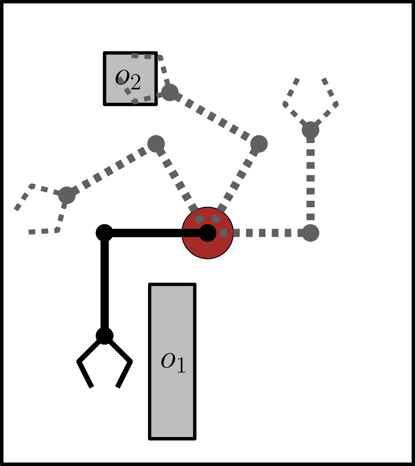
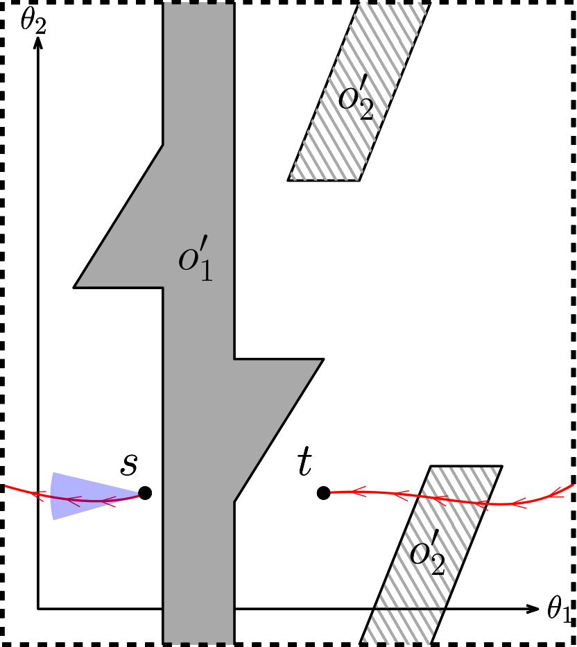
Consider the motion planning problem depicted in Figure 1, where a two joint planar manipulator must navigate from state to while avoiding obstacles . Now consider the related c-space in Figure 1(b), . Let be the guiding space whose heuristic is the distance to in , i.e., . As we will show next, this guiding space can be used to guide planning in .
A guiding space projection is a mapping from pairs of states in some search space to states of a guiding space . This mapping is conditioned on a search tree , which intuitively represents the known information regarding and . By relating tasks in to states in the projection allows a guided search algorithm to use the heuristic during search. Often for convenience we will drop the second term to the projection, namely .
In the example of Figure 1 the projection is . Note that this projection does not change the actual configuration , and only modifies its validity since configurations which collide only with obstacle in are valid in . Moreover, notice that despite colliding with obstacle , the path highlighted in red still contains useful information for computing paths in . First, the length of this path is a good estimate for the true global shortest path length, since a slight deviation is collision free and optimal. Second, regardless of global properties of the path, at certain configurations it contains locally near-optimal controls. The key insight is that not only does this path contain useful information, but also it is easier to compute than the true optimal solution, since it corresponds to a simpler search problem. The existence of quick to compute useful information is what motivates our definition of guided motion planning.
A guided motion planning problem is a motion planning problem augmented with a projection . We note that the image of describes a (potentially implicit) guiding space and corresponding . Next we formalize both how this information is used and where it comes from.
III-A Guided Search
Given a search tree , a baseline exploration algorithm might explore the space by selecting an existing state on the tree uniformly at random and then expanding from it according to some local planner. Unfortunately this approach has poor exploration properties, as it is heavily biased towards regions that have already been explored. Discrete search avoids this problem as newly explored states are checked against a cached set of visited states.
Algorithm 1 shows a guided search procedure for solving a problem . In each iteration the algorithm maps nodes on the tree through the projection then uses to determine the next node to explore, i.e., by selecting the node with minimum . In general, we can think of the projection as providing guidance by computing a distribution over the nodes of the tree from which we can sample to select how to expand. The tree then grows according to the neighborhood defined by the local planner. This parallels the well known heuristic guided discrete search algorithm A*.
III-B Computing a Guiding Space Projection
Consider an unknown but fixed distribution over robots, environments, and tasks. Guided search consists of an initial offline training phase, during which we train a projection on samples from this distribution. Note we are generally not concerned with time complexity during training, and that many algorithms skip this phase entirely. For example, RRT does not “train”, and performs the same procedure regardless of c-space. More commonly, after making assumptions about the c-space distribution, the human engineer encodes their prior knowledge into a suitable procedure for computing the projection, thus replacing the training phase. For example knowing that most obstacles in the environment are fixed might motivate projecting onto a guiding space in which collision with those obstacles has been precomputed [21]. Alternatively, knowing that some degree of freedom has negligible impact on might motivate projecting onto the other dimensions [24].
Next begins the online phase, in which a specific instantiation of a motion planning problem is sampled from the distribution and we conduct guided search on following Algorithm 1.
III-C Simple Examples of Guiding Spaces
One guiding space for is itself, , where is the identity and is the true distance to the goal configuration. This highlights the general setting in which a search space is used as a guiding space, in which for guidance to be useful we expect that solving tasks in be easier than in . Similarly, is a guiding space with a trivial projection and uninformed . Such trivial projections correspond to fixed sampling distributions over . We observe a natural trade-off between guidance quality and computation difficulty - computing solutions when is difficult (the original problem) but they provide perfect guidance, whereas when we can compute in constant time but get uninformed guidance.
The classic implementation of RRT samples uniformly in to select which node on the tree to expand. This is clearly not equivalent to sampling a node uniformly at random from the tree, and is known to consequently guide exploration towards unexplored regions via Voronoi bias. While in practice the guiding space is implicit in the sampling and nearest neighbor procedure, we can compute it explicitly through the Voronoi decomposition, where the value of each node on the tree is proportional to the volume of its corresponding cell. Notice how the guiding space depends on the search tree, as the nodes dictate the Voronoi cells.
As noted previously, a PRM in configuration space is a guiding space. If the distribution contains a single robot and environment, but is stochastic over tasks, then precomputing a discrete roadmap in is a common approach for answering multiple queries. The projection is often taken to be the function which returns the nearest neighbor on the graph. For any task and vertex , the heuristic is the length of the shortest path on the graph between and . This length is an approximation to the optimal solution for that task and can sometimes provide imperfect guidance; for example not every point in space might be locally navigable to a node on the graph.
IV Related work: categories of guidance
In this section we discuss existing work which does guided search. Note that many of the works cited below do not discuss guidance as a contribution, yet here we identify that they do implicitly perform guided search.
We separate guiding space methods into three main categories: robot modification, environment modification and experience based guidance. We find these subcategories natural and comprehensive, as the entire motion planning problem is encapsulated in the structure of the configuration space, which can be learned from experience, or is induced by its robot and environment constraints.
IV-A Robot Modification
Recalling that a configuration space is the product of a robot and environment , , we define robot modification as producing a guiding space for some new robot . In this paradigm, the projection function maps configurations in the first robot’s c-space to configurations in the second.
Given such a mapping , generally computes paths between configurations in . Notice that the translation of a path back into is often costly and may be one-to-many (e.g., inverse-kinematics), but isn’t necessary because we are only interested in the value of each state. It is then the job of the guided search algorithm to translate this value into feasible paths in .
There are many natural ways one might modify a robot description to obtain a closely related configuration space. One of the most natural projections is to define as workspace itself, ignoring the robot entirely and treating it as a fully controllable point robot in the environment [19, 13]. Some prior work ignores kinodynamic constraints on the robot [26], thereby yielding a guiding space where the robot is locally controllable. For chain-link robots, such as manipulators, a common guiding space involves focusing on a subset of the degrees of freedom [24]. Such methods often use heuristics in deciding which subsets to consider, e.g. focus on the first joints of a manipulator. Finally, some work attempts to learn a subspace of the robot’s degrees of freedom, e.g. using statistical projections such as PCA [25].
In general, we may think of robot modification methods as performing transfer learning in which examples of one robot performing tasks are used to inform plans for a second robot [14]. In the absence of a ground truth robot model, one can be learned from data [9].
All the above robot modification methods produce a search space as opposed to a guiding space. For example, workspace guidance methods often build a sparse graph in workspace, such as the medial axis [13]. Therefore there is often a secondary guided search that occurs in the modified robot space, e.g., the medial axis graph. This both highlights the hierarchical nature of guidance and helps isolate contributions - the medial axis is a useful structure for guiding search in workspace, and workspace is useful for guiding search in c-space.
IV-B Environment Modification
Environment modification refers to guiding spaces which map to . Unlike in robot modification, the associated projection is often simpler to compute, and translation of paths in back to requires relatively little work. In fact, in all work mentioned below, is nothing but the identity function, which only changes the validity of some points in to produce .
Narrow passages are a known bottleneck for randomized sampling algorithms. As such, some works modify obstacles in an attempt to widen passages [6, 29]. Lazy planning methods [10, 18] also perform a type of environment modification by ignoring constraints during initial planning, and incorporating them later as needed. When removing constraints, paths in are not necessarily valid in , and thus often such methods iteratively or hierarchically compute a guiding space (e.g., the initial lazy graph), use to produce samples near the unvalidated path, and then repeat with a new guiding space informed by the recently acquired samples (e.g., remove edges found to be invalid).
In contrast to the removal of environment constraints, adding constraints is less common, but can be done to simplify geometries and therefore collision detection [17]. Moreover, paths found when adding constraints are always valid in the original search space, and are thus easy to reuse. In other words, if we take to be the cost of paths in the modified space, constraint removal provides optimistic lower bounds whereas constraint addition produces conservative upper bounds.
IV-C Experience Based Guidance
The most common version of experience based guidance assumes the dataset contains a variety of environments all for the same robot. Consequently, database queries often consist of evaluating the degree to which paths in the dataset violate discovered constraints in the current motion planning instance [7]. While some methods only query using the task endpoints [12], more recent approaches propose to query (or filter) the database using local task features derived from workspace occupancy [11]. Another approach projects trajectories onto a lower dimensional abstract space via auto-encoding [20] or metrics like dynamic time warping [1], which improves database query.
Some methods perform multiple queries, where the guiding space effectively becomes the composite space of multiple independent motion planning problems from the dataset, e.g., through gaussian mixture models [11].
At the extreme end we have learning based methods which train a neural network from a dataset of experience to provide guidance, effectively combining all past solutions through the weights of the neurons of a neural network. In encoder-decoder models [27] we may think of the encoder as , which maps the input configuration space onto an abstract guiding space, and the decoder as , which solves the task in the abstract space to provide guidance, say through predicting cost-to-go [8]. Many learning based methods have poor generalization due to dependence on problem specific features, e.g., top down 2D occupancy maps [30]. Those with good generalization often scale poorly by learning an equivalent to cost-to-go [8], which even in a discrete space corresponds to computing or storing a prohibitively expensive all pairs shortest path.
In all learning based approaches a major challenge is gathering appropriate data, leading to methods which simplify the problem by learning local guidance through learned local planners [15]. Some work [5] proposes to gather appropriate data for training by using probabilistic roadmaps.
V Evaluation metric
V-A Sampling Efficiency
Often we evaluate sampling based motion planning methods using algorithm level holistic metrics such as running time or number of samples. While minimizing such metrics is a reasonable end goal, they can be sensitive to implementation details, and focusing on them can obscure which aspect of a proposed contribution is responsible for the results. In the context of guided motion planning, we now present a new method to evaluate quality of guidance.
In this work we focus on node selection as opposed to node expansion, and note that evaluating node expansion can be reduced to evaluating a node selection procedure between the set of possible expansions at a given node.
We propose to evaluate guidance by comparing the distribution of samples produced by the guiding space to some target distribution, namely one derived from an optimal sampling distribution with oracle access.
Definition 1 (Sampling efficiency)
Given a tree , a target sampling distribution over the tree nodes , and an empirical sampling distribution , the sampling efficiency of is defined as the information gain of using the target instead of , equivalently described as the Kullback-Liebler divergence between the two distributions,
When and are very similar is close to zero, and grows as they grow far apart. In the case where our empirical distribution is deterministic, , we have,
reducing to the negative log-likelihood of the empirical sample under the target distribution.
Intuitively, we aim to measure the difference between these two distributions, and while the KL-Divergence provides such a measure, it can be dominated by small regions in space where the two distributions have largest difference (e.g., when one distribution assigns zero probability to a region in which the other is non-zero). In sampling based motion planning we often aren’t worried about a few bad samples, so long as good ones are made with high enough probability so the bounded and symmetric Jensen-Shannon Divergence metric provides a smoother comparison, i.e.,
for mixture distribution . is therefore useful as it is less influenced by outliers in the distributions. Alternatively we can assume the target assigns a minimum nonzero probability to every node, for all , and therefore . In this way captures the maximum penalty we associate with poor sampling decisions made by the guiding space.
In shortest path problems we are interested in (efficiently) computing a boundedly optimal path in . Let be the suboptimality of , , where represents the distance between nodes on the tree and is the true shortest path between configurations in . Now let be the work remaining for a search starting at , . We propose to define with respect to these two quantities:
i.e., for temperature parameters which naturally balance the relative importance of optimality and efficiency. The smaller these parameters the steeper the distribution, assigning higher probability to samples with low and , and more heavily penalizing poor samples.
We can now define the smoothed as
where
V-B Axes for Evaluating Guidance
The metric described above measures the quality of each individual node expansion step of the guided search algorithm, but there are other options for evaluating guidance.
V-B1 Environment level
One can measure quality of guidance globally or in terms of local (possibly hierarchical) environment regions. In global evaluation we take an expectation of quality over tasks sampled from the environment. In local evaluation we subdivide the environment and compute our metric on each region independently, reporting the distribution of results over the full environment. Note that our method for global evaluation naturally applies to any subdivision of the environment, and we leave a discussion of appropriate environment partitioning to future work.
V-B2 Sample level
One can measure quality of guidance by considering both single and multiple samples. In single-step evaluation we measure the expected quality of a single node expansion of a single search tree. Such evaluation not only depends on the task and environment, but on the current exploration progress, namely information regarding previously sampled points in the configuration space encoded in the search tree. In multiple-sample evaluation we instead measure the holistic efficiency of all samples produced by the guiding space over the course of planning.
In other words, single-step evaluation considers distributions over trees , whereas in multiple-sample evaluation considers distributions over , implicitly described by the distribution of valid trees produced by an algorithm. We refer the reader to [4] for a more in depth discussion of multiple-sample evaluation, and here summarize that in that setting our metric reduces to measuring the entropy of the observed sampling distribution. In this case lower entropy means better guidance.
VI Refactoring Existing Algorithms
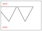
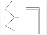
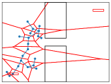
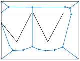
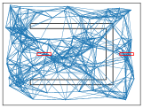
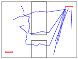
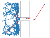
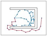
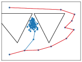
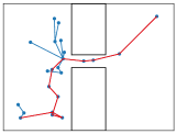
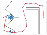
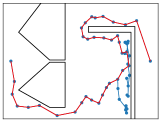
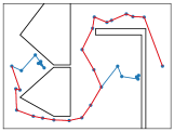
Existing algorithms such as those cited in Section IV are not implemented in the form of Algorithm 1, rather each uses their respective guiding space in a different way. In the next section we conduct experiments on four guided search algorithms, RRT [23], LazyPRM [10], DR-RRT [13], and Lightning [7]. Figure 4 shows examples of trees produced by these algorithms for solving the tasks depicted in Figure 2, and Figure 3 visualizes their guiding spaces.
LazyPRM builds a probabilistic roadmap without performing collision detection with the environment (or only doing so for vertices but not edges). Our implementation grows a tree using the length of the shortest path on this lazy graph as guidance for selecting which node to expand on the tree. When an invalid sample is found in c-space, we pass this information back to the guiding space (the lazy graph) by deleting nearby vertices/edges.
DR-RRT uses the medial axis skeleton computed in workspace to guide the robot. The original proposed implementation uses the edges of this skeleton to define “dynamic regions” along which to sample, and does so by creating balls around these regions and projecting back into c-space. For robots whose workspace configuration is a subset of the dimensions of their c-space this is easy, but for more complex c-space the general form of such a procedure involves an inverse-kinematics projection. Our new implementation, which we call MedialAxisGuidance is more straightforward - we project c-space nodes with forward-kinematics into workspace, then project these workspace poses onto the nearest medial axis edge . The corresponding guidance value is then the distance along the skeleton edges from the projected edge to the projection of the goal, . Whenever a node fails to expand due to obstacle collision we increase the weight of , thereby reducing the chance that the guidance encourages exploration along that edge.
Lightning uses a database of paths from related motion planning problems to guide exploration. Namely, given a motion planning problem, a path that was produced by the most similar task (start and goal) is selected from the database, and then copied into the current c-space. Where the path is invalid the algorithm fixes the solution by running a bi-directional RRT from the two ends of the breakage. We highlight that this sub-problem can be just as difficult as the original, and moreover that the full power of the database is never used. Our new implementation, which we call PathDatabaseGuidance uses the length of the queried path as the guidance value. As with LazyPRM, failed sample information is passed down to the guiding space by filtering out paths that pass close to invalid regions. If no node can locally plan to any path, then we default to RRT until a new node is found from which there is a visible path. We note that this implementation is relatively similar to [1], but we query the database using task similarity as in [7] rather than dynamic time warping, and more importantly we actively filter the database using information from the search tree.
VII Experiments
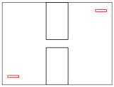
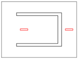
We design environments intended to demonstrate both pros and cons of each guiding space mentioned in Section VI, using a rectangular mobile base (3-dimensional c-space) in a 2-dimensional workspace.
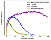
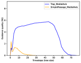
We show results in Figure 5, plotting quality of guidance (lower is better) over the course of search progress, i.e., number of samples. RRT initially performs similarly on all environments, doing well and then poorly as it struggles to get through narrow passages. LazyPRM performs well on SimplePassage but poorly on Cup, where it spends time exploring the dead end. MedialAxisGuidance does well on SimplePassage but poorly on Trap, where a valid passage in workspace is not valid in c-space. These first three experiments demonstrate that guidance matches our intuition for when each algorithm performs well or struggles, which can be seen qualitatively in Figure 4. In addition, we highlight that RRT is comparable to other algorithms initially, and especially on environments where MedialAxisGuidance or LazyPRM lead the search astray.
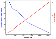
Next we test PathDatabaseGuidance on a dataset of RandomSimplePassages, an environment with a randomly placed narrow passage between two rooms. We show how guidance improves as dataset size increases, while runtime gets worse (as querying the database takes longer), showing how such traditional metrics can obscure properties of algorithms because they are implementation dependent. This matches the intuition mentioned in Section III-C regarding the trade-off between guidance quality and the difficulty of computing it.
VII-A Multi-guidance search
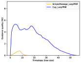
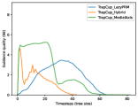
Finally, we create a hybrid environment TrapCup which combines features form both the Trap and Cup environments. We now design a hybrid guiding space that is a combination of LazyPRM and MedialAxis. In other words, it creates both guiding spaces (i.e., the cross product) and uses a rule to determine how to select or combine the heuristics from the two. In the experiments shown in Figure 6 we simply swap the source of the guidance each time the search collides with an obstacle. Intuitively, each form of guidance faces certain local minima and by using multiple guiding spaces we can quickly escape those minima by passing control to another guiding space. Notice that the individual guidance plots for each guiding space indicate that these local minima are distinct (e.g., the curves have different peaks), and thus we see the hybrid guiding space out-performs its parts. Moreover, using number of samples alone as a metric would obscure this fact since MedialAxis and LazyPRM take about the same number of samples to find the goal. These results parallel what one would expect from running a multi-heuristic A* search [2] as opposed to single heuristic search, and highlights the value of framing sampling based motion planning as guided search; we now have a structured way of combining different algorithmic ideas from the literature as multiple guiding spaces, whereas the original implementation are not so conducive to modularization.
VIII Conclusion
In this work we presented the guiding space framework, in which an explicit guiding space provides heuristic guidance to a tree based search algorithm in a configuration space. We showed how many existing methods fit this framework, albeit implicitly. By viewing such methods as guiding spaces, we can more easily compare and combine them into hybrid algorithms. As such, we defined sampling efficiency as a way to measure the quality of biased node selections of a search tree, and showed how this metric matches intuition for a variety of algorithms and environments.
References
- [1] Sandip Aine, Charupriya Sharma, and Maxim Likhachev. Learning to search more efficiently from experience: A multi-heuristic approach. In Proceedings of the International Symposium on Combinatorial Search, volume 6, pages 141–145, 2015.
- [2] Sandip Aine, Siddharth Swaminathan, Venkatraman Narayanan, Victor Hwang, and Maxim Likhachev. Multi-heuristic a. The International Journal of Robotics Research, 35(1-3):224–243, 2016.
- [3] Nancy M Amato, O Burchan Bayazit, Lucia K Dale, Christopher Jones, Daniel Vallejo, et al. Obprm: An obstacle-based prm for 3d workspaces. In Proc. Int. Workshop on Algorithmic Foundations of Robotics (WAFR), pages 155–168, 1998.
- [4] Amnon Attali, Stav Ashur, Isaac Burton Love, Courtney McBeth, James Motes, Diane Uwacu, Marco Morales, and Nancy M Amato. Evaluating guiding spaces for motion planning. arXiv preprint arXiv:2210.08640, 2022.
- [5] Amnon Attali, Marco Morales, and Nancy M Amato. Discrete state-action abstraction via the successor representation. arXiv preprint arXiv:2206.03467, 2022.
- [6] O. Burçhan Bayazit, Dawen Xie, and Nancy M. Amato. Iterative relaxation of constraints: a framework for improving automated motion planning. In 2005 IEEE/RSJ International Conference on Intelligent Robots and Systems, 2005, pages 3433–3440. IEEE, 2005.
- [7] Dmitry Berenson, Pieter Abbeel, and Ken Goldberg. A robot path planning framework that learns from experience. In 2012 IEEE International Conference on Robotics and Automation, pages 3671–3678. IEEE, 2012.
- [8] Mohak Bhardwaj, Sanjiban Choudhury, and Sebastian Scherer. Learning heuristic search via imitation. In Conference on Robot Learning, pages 271–280. PMLR, 2017.
- [9] Botond Bocsi, Lehel Csató, and Jan Peters. Alignment-based transfer learning for robot models. In The 2013 international joint conference on neural networks (IJCNN), pages 1–7. IEEE, 2013.
- [10] Robert Bohlin and Lydia E. Kavraki. Path planning using lazy PRM. In International Conference on Robotics and Automation, ICRA, pages 521–528. IEEE, 2000.
- [11] Constantinos Chamzas, Zachary Kingston, Carlos Quintero-Peña, Anshumali Shrivastava, and Lydia E Kavraki. Learning sampling distributions using local 3d workspace decompositions for motion planning in high dimensions. In 2021 IEEE International Conference on Robotics and Automation (ICRA), pages 1283–1289. IEEE, 2021.
- [12] David Coleman, Ioan A Şucan, Mark Moll, Kei Okada, and Nikolaus Correll. Experience-based planning with sparse roadmap spanners. In 2015 IEEE International Conference on Robotics and Automation (ICRA), pages 900–905. IEEE, 2015.
- [13] Jory Denny, Read Sandström, Andrew Bregger, and Nancy M. Amato. Dynamic region-biased rapidly-exploring random trees. In Proceedings of the Twelfth Workshop on the Algorithmic Foundations of Robotics, WAFR 2016,, volume 13 of Springer Proceedings in Advanced Robotics, pages 640–655. Springer, 2016.
- [14] Coline Devin, Abhishek Gupta, Trevor Darrell, Pieter Abbeel, and Sergey Levine. Learning modular neural network policies for multi-task and multi-robot transfer. In 2017 IEEE international conference on robotics and automation (ICRA), pages 2169–2176. IEEE, 2017.
- [15] Aleksandra Faust, Kenneth Oslund, Oscar Ramirez, Anthony Francis, Lydia Tapia, Marek Fiser, and James Davidson. Prm-rl: Long-range robotic navigation tasks by combining reinforcement learning and sampling-based planning. In 2018 IEEE international conference on robotics and automation (ICRA), pages 5113–5120. IEEE, 2018.
- [16] Roland Geraerts and Mark H Overmars. Creating high-quality paths for motion planning. The international journal of robotics research, 26(8):845–863, 2007.
- [17] Mukulika Ghosh, Shawna L. Thomas, Marco Morales, Samuel Rodríguez, and Nancy M. Amato. Motion planning using hierarchical aggregation of workspace obstacles. In 2016 IEEE/RSJ International Conference on Intelligent Robots and Systems, pages 5716–5721. IEEE, 2016.
- [18] Kris Hauser. Lazy collision checking in asymptotically-optimal motion planning. In IEEE International Conference on Robotics and Automation, ICRA 2015, Seattle, WA, USA, 26-30 May, 2015, pages 2951–2957. IEEE, 2015.
- [19] Christopher Holleman and Lydia E Kavraki. A framework for using the workspace medial axis in prm planners. In IEEE International Conference on Robotics and Automation, volume 2, pages 1408–1413. IEEE, 2000.
- [20] Brian Ichter and Marco Pavone. Robot motion planning in learned latent spaces. IEEE Robotics and Automation Letters, 4(3):2407–2414, 2019.
- [21] Léonard Jaillet and Thierry Siméon. A prm-based motion planner for dynamically changing environments. In 2004 IEEE/RSJ International Conference on Intelligent Robots and Systems (IROS)(IEEE Cat. No. 04CH37566), volume 2, pages 1606–1611. IEEE, 2004.
- [22] Lydia E. Kavraki, Petr Svestka, Jean-Claude Latombe, and Mark H. Overmars. Probabilistic roadmaps for path planning in high-dimensional configuration spaces. IEEE Trans. Robotics Autom., 12(4):566–580, 1996.
- [23] Steven LaValle. Rapidly-exploring random trees: A new tool for path planning. Research Report 9811, 1998.
- [24] Tomas Lozano-Perez. A simple motion-planning algorithm for general robot manipulators. IEEE Journal on Robotics and Automation, 3(3):224–238, 1987.
- [25] Arthur Mahoney, Joshua Bross, and David Johnson. Deformable robot motion planning in a reduced-dimension configuration space. In IEEE International Conference on Robotics and Automation, ICRA 2010, pages 5133–5138. IEEE, 2010.
- [26] Erion Plaku, Lydia E. Kavraki, and Moshe Y. Vardi. Discrete search leading continuous exploration for kinodynamic motion planning. In Robotics: Science and Systems III, 2007. The MIT Press, 2007.
- [27] Ahmed H Qureshi, Anthony Simeonov, Mayur J Bency, and Michael C Yip. Motion planning networks. In 2019 International Conference on Robotics and Automation (ICRA), pages 2118–2124. IEEE, 2019.
- [28] Kensen Shi, Jory Denny, and Nancy M Amato. Spark prm: Using rrts within prms to efficiently explore narrow passages. In 2014 IEEE International Conference on Robotics and Automation (ICRA), pages 4659–4666. IEEE, 2014.
- [29] Vojtech Vonásek, Robert Penicka, and Barbora Kozlíková. Computing multiple guiding paths for sampling-based motion planning. In 19th International Conference on Advanced Robotics, ICAR 2019, pages 374–381. IEEE, 2019.
- [30] Jiankun Wang, Wenzheng Chi, Chenming Li, Chaoqun Wang, and Max Q-H Meng. Neural rrt*: Learning-based optimal path planning. IEEE Transactions on Automation Science and Engineering, 17(4):1748–1758, 2020.