A primal-dual adaptive finite element method for total variation based motion estimation

Abstract

Based on previous work we extend a primal-dual semi-smooth Newton method for minimizing a general $L^{1}$-$L^{2}$-$TV$ functional over the space of functions of bounded variations by adaptivity in a finite element setting. For automatically generating an adaptive grid we introduce indicators based on a-posteriori error estimates. Further we discuss data interpolation methods on unstructured grids in the context of image processing and present a pixel-based interpolation method. For the computation of optical flow we derive an adaptive finite element coarse-to-fine scheme for resolving large displacements. The coarse-to-fine scheme speeds-up the computing time tremendously.

1 Introduction

Let $\Omega\subseteq\mathbb{R}^{d}$, $d\in\mathbb{N}$, be an open, bounded and simply connected domain with Lipschitz boundary. We consider the problem of minimizing the $L^{1}$-$L^{2}$-TV functional [22], which has various applications in image processing and has been subject of study in [24, 25] and in a finite element context in [2]. More precisely, as in [21] we consider it in the following form

$$\inf_{\mathbf{u}\in V}\Big{\{}\alpha_{1}\int_{\Omega}\varphi_{\gamma_{1}}(|T\mathbf{u}-g|)\;\mathrm{d}\mathbf{x} +\tfrac{\alpha_{2}}{2}\|T\mathbf{u}-g\|_{L^{2}}^{2}+\tfrac{\beta}{2}\|S\mathbf{u}\|_{V_{S}}^{2}$$ (1)

$$+\lambda\int_{\Omega}\varphi_{\gamma_{2}}(|D\mathbf{u}|_{F})\;\mathrm{d}\mathbf{x}=:E(\mathbf{u})\Big{\}},$$

where $V:=H^{1}(\Omega)^{m}$, $m\in\mathbb{N}$, is a continuously embedded Hilbert space, $S:V\to V_{S}$ is a bounded linear operator for some Hilbert space $V_{S}$, $T:L^{2}(\Omega)^{m}\to L^{2}(\Omega)$ is a bounded linear operator, $g\in L^{2}(\Omega)$ is some given data, $|\operatorname{\,\cdot\,}|_{F}:\mathbb{R}^{d\times m}\mapsto\mathbb{R}$ denotes the Frobenius norm, and $\alpha_{1},\alpha_{2},\lambda,\beta\geq 0$ are adjustable weighting parameters. Further $\gamma_{1},\gamma_{2}\geq 0$ are Huber-regularization parameters associated to the Huber-function $\varphi_{\gamma}:\mathbb{R}\to[0,\infty)$ for $\gamma\geq 0$ defined by

$$\varphi_{\gamma}(x):=\begin{cases}\mathchoice{\tfrac{1}{2\gamma}}{\frac{1}{2\gamma}}{\frac{1}{2\gamma}}{\frac{1}{2\gamma}}x^{2}&\text{if }|x|\leq\gamma,\\ |x|-\mathchoice{\tfrac{\gamma}{2}}{\frac{\gamma}{2}}{\frac{\gamma}{2}}{\frac{\gamma}{2}}&\text{if }|x|>\gamma.\end{cases}$$ (2)

We remark that $d$ denotes the spatial dimension, e.g. one sets $d=1$ for signals and $d=2$ for images, and $m$ describes the number of channels, i.e. for grey-scale images $m=1$ and for motion fields we have $m=d$. In [21] a primal-dual framework around 1 has been developed and a finite element semi-smooth Newton scheme established. The present work aims to extend [21] to an adaptive finite element setting and considers the image analysis problem of estimating the optical flow in image sequences. Note that we set $V=H^{1}(\Omega)^{m}$, although in general a solution of 1 can only be guaranteed in $L^{2}(\Omega)^{m}$, see section 2.2 below for more details. However, any of these solutions can be approximated by continuous piecewise linear finite elements [7, Chapter 10.2]. Since all such discrete functions are elements of $H^{1}(\Omega)^{m}$ and in this paper we are interested in developing an adaptive finite element scheme for 1, it seems sufficient to us to set $V=H^{1}(\Omega)^{m}$ from the beginning. Moreover, we note that the finite element semi-smooth Newton scheme in [21] is also derived for this space setting.

Related work

While mathematical image processing techniques are often presented or discretized in a finite difference setting due to simple handling of image array data, finite element methods in image processing have also been studied, see [16] for an overview. The ability to adaptively refine or coarsen unstructured finite element meshes seems promising in order to save computational resources during processing. We refer the reader to [27, 30] for an overview of adaptive finite element methods. We note that images usually have homogeneous regions as well as parts with a lot of details. It seems intuitively sufficient to discretize fine in regions of transitions and fine details, while a coarse discretisation should do well in uniform parts. To this end error estimates are crucial in order to correctly guide the refinement process. First attempts for using adaptive finite element methods in image processing (restoration) have been made for non-linear diffusion models, which are mainly used for image denoising and edge detection. In particular, in [4, 9, 28] adaptive finite element methods are proposed for the modified Perona-Malik model [15]. Based on primal-dual gap error estimators adaptive finite element methods for the $L^{2}$-TV model, i.e. 1 with $\alpha_{1}=\beta=\gamma_{2}=0$, are proposed in [6, 8]. While in [6] the dual problem is discretized by continuous, piecewise affine finite elements, in [8] the Brezzi-Douglas-Morini finite elements [14] are used. Note that in [6, 8] only clean images are considered and no image reconstruction or analysis problem is tackled. In a similar way relying on a semi-smooth Newton method for minimizing the $L^{2}$-TV model over the Hilbert space $H^{1}_{0}(\Omega)$ in [23] an adaptive finite element method, again using a posteriori error estimates, is suggested for image denoising only. Adaptive finite element methods for optical flow computation have been presented in [10, 11]. However, these methods differ significantly from our approaches. Firstly, a different minimization problem is considered. Secondly, the mesh in the methods in [10, 11] is initialized at fine image resolution and iteratively coarsened only after a costly computation, while our approach allows to start with a coarse mesh and refines cells only if deemed necessary.

On this work

In the present work we extend the finite element framework of [21] to an adaptive finite element setting and consider the application of motion estimation. The proposed adaptive finite element method is based on a-posteriori error estimates. For deriving the residual-based error estimates we do not consider a variation inequality setting as in [23] but utilize the strong convexity of the functional in 1. Further, while the approach in [23] only considers the image denoising case, i.e.  $T$ being the identity, our estimate allows for general linear and bounded operators $T$. Utilizing our derived a-posteriori estimators allows us to propose an adaptive scheme for estimating motion in image sequences. More precisely, we incorporate into [21, Algorithm 3] an adaptive coarse-to-fine warping scheme for optical flow computation which makes use of the developed adaptive finite element framework and is able to resolve large displacements. In particular, due to the adaptive coarse-to-fine warping scheme the proposed algorithm improves [21, Algorithm 3] in two directions. Firstly, it produces more accurate approximations of the optical flow and secondly, it significantly reduces the computing time.

Note that for finite elements in general an interpolation method needs to be employed to transfer given data onto a finite element function. The choice of this method is especially relevant when the underlying grid is coarser than the original image resolution since in that case e.g. nodal sampling for standard linear Lagrange finite elements can lead to aliasing artifacts. In this vein, we propose a new pixel-adapted method to interpolate image data onto finite element meshes and compare it to other alternatives. This new method is designed to minimize the discrete $\ell^{2}$-distance to the original image on the original image grid. That is, it actually optimizes the peak signal-to-noise ratio ($\operatorname{PSNR}$) and therefore might be especially suited for images.

The rest of the paper is organized as follows: In section 2 we fix the basic notation and terminology used and describe the primal-dual setting of 1. Based on this primal-dual formulation we introduce in section 3 our finite element setting. The main part of this section is devoted to the derivative of a-posteriori error estimates to establish an adaptive finite element algorithm for 1. Moreover, we describe several different image interpolation methods and compare them with a newly proposed pixel-adapted interpolation method. Based on the developed adaptive finite element method in section 4 an adaptive coarse-to-fine warping scheme for motion estimation is proposed and its applicability to detect large displacements on image sequences is demonstrated.

2 Preliminaries

2.1 Notation and Terminology

For a Hilbert space $H$ we denote by $\langle\operatorname{\,\cdot\,},\operatorname{\,\cdot\,}\rangle_{H}$ its inner product and by $\|\operatorname{\,\cdot\,}\|_{H}$ its induced norm. The duality pairing between $H$ and its continuous dual space $H^{*}$ is written as $\langle\operatorname{\,\cdot\,},\operatorname{\,\cdot\,}\rangle_{H,H^{*}}$. In the case $H=L^{2}(\Omega)^{n}$, $n\in\mathbb{N}$, we define the associated inner product by $\langle\operatorname{\,\cdot\,},\operatorname{\,\cdot\,}\rangle_{H}:\big{(}(u_{k})_{k=1}^{n},(v_{k})_{k=1}^{n}\big{)}\mapsto\sum_{k=1}^{n}\langle u_{k},v_{k}\rangle_{L^{2}(\Omega)}$, where $\langle\operatorname{\,\cdot\,},\operatorname{\,\cdot\,}\rangle_{L^{2}(\Omega)}$ is the standard $L^{2}$ inner product. Apart from notational convenience, we treat a matrix-valued space $L^{2}(\Omega)^{d\times m}$ as equivalent to $L^{2}(\Omega)^{dm}$ using the numbering $(i,j)\mapsto(j-1)\cdot d+i$, $i\in\{1,\dotsc,d\}$, $j\in\{1,\dotsc,m\}$ of the respective components. Moreover, for any $L^{2}$ function space we may use the inner product shorthand notations $\langle\operatorname{\,\cdot\,},\operatorname{\,\cdot\,}\rangle_{L^{2}}:=\langle\operatorname{\,\cdot\,},\operatorname{\,\cdot\,}\rangle_{H}$ and similarly $\|\operatorname{\,\cdot\,}\|_{L^{2}}:=\|\operatorname{\,\cdot\,}\|_{H}$ for the norm. In the sequel, the dual space $H^{*}$ of a Hilbert space $H$ will often be identified with itself.

For a bounded linear operator $\Lambda\in\mathcal{L}(X,Y)$, where $X,Y$ are Hilbert spaces, we define by $\|\Lambda\|:=\|\Lambda\|_{\mathcal{L}(X,Y)}$ its operator norm and denote by $\Lambda^{*}:Y^{*}\to X^{*}$ its adjoint operator. In the sequel by single strokes, i.e. $|\operatorname{\,\cdot\,}|$, we describe the Euclidean norm on $\mathbb{R}^{n}$, $n\in\mathbb{N}$. Often operations are applied in a pointwise sense, such that for a vector-valued function $\mathbf{u}:\Omega\to\mathbb{R}^{m}$ the expression $|\mathbf{u}|$ denotes the function $|\mathbf{u}|:\Omega\to\mathbb{R}$, $\mathbf{x}\mapsto|\mathbf{u}(\mathbf{x})|$.

A function $f:H\to\overline{\mathbb{R}}:=\mathbb{R}\cup\{+\infty\}$ is called coercive, if for any sequence $(\mathbf{v}_{n})_{n\in\mathbb{N}}\subseteq H$ we have

$$\|\mathbf{v}_{n}\|_{H}\to\infty\implies f(\mathbf{v}_{n})\to\infty.$$

A bilinear form $a:H\times H\to\mathbb{R}$ is called coercive, if there exists a constant $c>0$ such that $a(\mathbf{v},\mathbf{v})\geq c\|\mathbf{v}\|^{2}_{H}$ for all $\mathbf{v}\in H$. The subdifferential for a convex function $f:X\to\overline{\mathbb{R}}:=\mathbb{R}\cup\{+\infty\}$ at $\mathbf{v}\in X$ is defined as the set valued function

$$\partial f(\mathbf{v})=\begin{cases}\emptyset&\text{if }f(\mathbf{v})=\infty,\\ \{\mathbf{v}^{*}\in X^{*}:\langle\mathbf{v}^{*},\mathbf{u}-\mathbf{v}\rangle_{X^{*},X}+f(\mathbf{v})\leq f(\mathbf{u})\ \forall\mathbf{u}\in X\}&\text{otherwise}.\end{cases}$$

Further for a predicate $w:\Omega\to\{\mathrm{true},\mathrm{false}\}$ we define the indicator $\chi_{w}\in\overline{\mathbb{R}}$ as

$$\chi_{w}:=\begin{cases}0&\text{if $w(\mathbf{x})$ is true for almost every\ $\mathbf{x}\in\Omega$},\\ \infty&\text{else}.\end{cases}$$

For example, let $u\in L^{2}(\Omega)$, then $\chi_{|u|\leq 1}$ would evaluate to $\infty$ if and only if $|u|$ is greater than $1$ on a set of non-zero measure.

2.2 Primal-Dual Formulation

Let us recall the functional setting and the primal-dual formulation of [21], on which our derived a-posteriori estimates and hence our proposed adaptive finite element scheme, presented in section 3 below, are based. We restrict ourselves for the operator $S$ in 1 and its related spaces to the following two settings:

1. $S:=I:V\to V_{S}$ with $\|\operatorname{\,\cdot\,}\|_{V}:=\|\operatorname{\,\cdot\,}\|_{H^{1}}$ and $V_{S}=L^{2}(\Omega)^{m}$, $\|\operatorname{\,\cdot\,}\|_{V_{S}}:=\|\operatorname{\,\cdot\,}\|_{L^{2}}$ or

2. $S:=\nabla:V\to V_{S}$ with $\|\operatorname{\,\cdot\,}\|_{V}:=\|\operatorname{\,\cdot\,}\|_{H^{1}}$ and $V_{S}=L^{2}(\Omega)^{d\times m}$ (the boundedness of $S$ follows due to $\|\nabla\mathbf{v}\|_{L^{2}}\leq\|\mathbf{v}\|_{H^{1}}$), $\|\operatorname{\,\cdot\,}\|_{V_{S}}:=\|\operatorname{\,\cdot\,}\|_{L^{2}}$.

Note that items ($S$.i) and ($S$.ii) here differ from the ones in [21]. The reason is that here $V=H^{1}(\Omega)$ is fixed and in our discretisation, see section 3 below, our finite dimensional space $V_{h}$ is a subspace of $H^{1}(\Omega)^{m}$ and not a subspace of a subspace of $L^{2}(\Omega)^{m}$ and $H^{1}(\Omega)^{m}$, as in [21].

We define the symmetric bilinear form $a_{B}:V\times V\to\mathbb{R}$ by

$$a_{B}(\mathbf{u},\mathbf{w}):=\alpha_{2}\langle T\mathbf{u},T\mathbf{w}\rangle_{L^{2}}+\beta\langle S\mathbf{u},S\mathbf{w}\rangle_{L^{2}}=\langle B\mathbf{u},\mathbf{w}\rangle_{V^{*},V},$$ (3)

whereby $B:=\alpha_{2}T^{*}T+\beta S^{*}S:V\to V^{*}$. The bilinear form $a_{B}$ induces a respective energy norm defined by

$$\|\mathbf{u}\|_{B}^{2}:=a_{B}(\mathbf{u},\mathbf{u})\qquad\text{for}\ \mathbf{u}\in V.$$

To guarantee the existence of a (unique) solution of 1 in the sequel we assume that $a_{B}$ is coercive [21, Proposition 3.1]:

1. The bilinear form $a_{B}:V\times V\to\mathbb{R}$ is coercive.

Here the coercivity is to be understood in the following ways according to item ($S$.i) and item ($S$.ii): In item ($S$.i) the coercivity is with respect to the $L^{2}$-norm, i.e. $a_{B}$ is $L^{2}$-coercive, and hence a solution is (only) ensured in $L^{2}(\Omega)^{m}$. This is, as in this case coercivity with respect to the $H^{1}$-norm seems too restrictive and may only hold in very special cases. For item ($S$.ii) the coercivity is understood with respect to $\|\cdot\|_{V}$ (i.e. the $H^{1}$-norm) which guarantees a solution in $V$.

Replacing $V$ by a finite dimensional subspace of $L^{2}(\Omega)^{m}$ in item ($S$.i) or $V$ in item ($S$.ii), then (A1) guarantees a solution in the respective finite dimensional space [21]. Further, the coercivity of $a_{B}$ implies the invertibility of $B$ [21, Remark 2.1]. Accordingly, we define the norm $\|\mathbf{u}\|_{B^{-1}}^{2}:=\langle\mathbf{u},{B^{-1}}\mathbf{u}\rangle_{V^{*},V}$ for $\mathbf{u}\in V^{*}$. Additionally, we introduce the linear and bounded operator $\Lambda:=(T,\nabla):V\to W:=L^{2}(\Omega)\times L^{2}(\Omega)^{d\times m}$.

In these settings we recall the following duality result.

Theorem 2.1 ([21, Theorem 3.1 $\&$ Proposition 3.2]).

The pre-dual problem to 1 reads

$$\inf_{\mathbf{p}=(p_{1},\mathbf{p}_{2})\in W^{*}}\;\Big{\{}\tfrac{1}{2}\big{\|}\Lambda^{*}\mathbf{p}- \alpha_{2}T^{*}g\big{\|}_{B^{-1}}^{2}-\tfrac{\alpha_{2}}{2}\|g\|_{L^{2}}^{2}+\langle g,p_{1}\rangle_{L^{2}}+\chi_{|p_{1}|\leq\alpha_{1}}$$ (4)

$$+\tfrac{\gamma_{1}}{2\alpha_{1}}\|p_{1}\|_{L^{2}}^{2}+\chi_{|\mathbf{p}_{2}|_{F}\leq\lambda}+\tfrac{\gamma_{2}}{2\lambda}\|\mathbf{p}_{2}\|_{L^{2}}^{2}=:D(\mathbf{p})\Big{\}},$$

where for $\alpha_{1}=0$ or $\lambda=0$ we use the convention that the terms $\tfrac{\gamma_{1}}{2\alpha_{1}}\|p_{1}\|_{L^{2}}^{2}$ and $\tfrac{\gamma_{2}}{2\lambda}\|\mathbf{p}_{2}\|_{L^{2}}^{2}$ vanish respectively.

Furthermore, solutions $p=(p_{1},\mathbf{p}_{2})\in W^{*}$ and $\mathbf{u}\in V$ of 4 and 1 respectively are characterized by

$$0 =\Lambda^{*}\mathbf{p}-\alpha_{2}T^{*}g+B\mathbf{u},$$ (5)

$$0 =p_{1}\max\{\gamma_{1},|T\mathbf{u}-g|\}-\alpha_{1}(T\mathbf{u}-g), |p_{1}| \leq\alpha_{1},$$

$$0 =\mathbf{p}_{2}\max\{\gamma_{2},|\nabla\mathbf{u}|_{F}\}-\lambda\nabla\mathbf{u}, |\mathbf{p}_{2}|_{F} \leq\lambda,$$

where $\max$ denotes the pointwise maximum.

The primal functional $E$ from 1 satisfies the following strong convexity property.

Lemma 2.2.

If $\hat{\mathbf{u}}\in V$ is a minimizer of $E$, then we have

$$\tfrac{1}{2}\|\mathbf{u}-\hat{\mathbf{u}}\|_{B}^{2}\leq E(\mathbf{u})-E(\hat{\mathbf{u}})$$

for all $\mathbf{u}\in V.$

Proof.

We apply the same method as in [5, Lemma 10.2]. For the energy $E$ from 1 we write $E(\mathbf{u})=F(\mathbf{u})+G(\mathbf{u})$ with

$$G(\mathbf{u}):=\alpha_{1}\int_{\Omega}\varphi_{\gamma_{1}}(|T\mathbf{u}-g|)\;\mathrm{d}\mathbf{x}+\lambda\int_{\Omega}\varphi_{\gamma_{2}}(|D\mathbf{u}|_{F})\;\mathrm{d}\mathbf{x}$$

and

$$F(u):=\tfrac{\alpha_{2}}{2}\|T\mathbf{u}-g\|_{L^{2}}^{2}+\tfrac{\beta}{2}\|S\mathbf{u}\|_{L^{2}}^{2}.$$

Note that $F$ is Frechet-differentiable with

$$\langle F^{\prime}(\mathbf{u}),\mathbf{w}\rangle_{V^{*},V}=\alpha_{2}\langle T\mathbf{u}-g,T\mathbf{w}\rangle_{L^{2}}+\beta\langle S\mathbf{u},S\mathbf{w}\rangle_{L^{2}}$$

for all $\mathbf{w}\in V$. Expanding $F(\mathbf{u})$ at $\hat{\mathbf{u}}$ then yields

$$F(\mathbf{u})=F(\hat{\mathbf{u}})+\langle F^{\prime}(\hat{\mathbf{u}}),\mathbf{u}-\hat{\mathbf{u}}\rangle_{V^{*},V}+\tfrac{1}{2}\|\mathbf{u}-\hat{\mathbf{u}}\|_{B}^{2}.$$

Since $\hat{u}\in V$ is a minimizer, we have $0\in\partial E(\hat{\mathbf{u}})=F^{\prime}(\hat{\mathbf{u}})+\partial G(\hat{\mathbf{u}})$. Hence $-F^{\prime}(\hat{\mathbf{u}})\in\partial G(\hat{\mathbf{u}})$, i.e.

$$\langle-F^{\prime}(\hat{\mathbf{u}}),\mathbf{u}-\hat{\mathbf{u}}\rangle_{V^{*},V}\leq G(\mathbf{u})-G(\hat{\mathbf{u}})$$

and thus

$$\tfrac{1}{2}\|\mathbf{u}-\hat{\mathbf{u}}\|_{B}^{2}\leq F(\mathbf{u})-F(\hat{\mathbf{u}})+G(\mathbf{u})-G(\hat{\mathbf{u}}),$$

which proves the statement. ∎

Putting lemma 2.2 and coercivity of $a_{B}$ from item (A1) together we obtain that for a minimizer $\mathbf{u}$ of $E$ there is a constant $c>0$ such that

$$E(\mathbf{v})-E(\mathbf{u})\geq\tfrac{1}{2}\|\mathbf{u}-\mathbf{v}\|_{B}^{2}=\begin{cases}\tfrac{c}{2}\|\mathbf{u}-\mathbf{v}\|_{L^{2}}^{2}&\text{for \lx@cref{creftype~refnum}{setting-identity}}\\ \tfrac{c}{2}\|\mathbf{u}-\mathbf{v}\|_{H^{1}}^{2}&\text{for \lx@cref{creftype~refnum}{setting-nabla}}\end{cases}$$

for all $\mathbf{v}\in V$.

3 Discretization: Finite Elements

Central to the idea of finite element discretization is the idea to find a solution within a finite dimensional subspace of the original space. This discrete space usually consists of cellwise polynomial functions defined on a mesh of cells, e.g. simplices. In contrast to finite differences the discretization may be adaptively refined to accomodate certain local error indicators, thereby reducing the amount of degrees of freedom needed to represent a solution up to a certain accuracy. For more details on adaptive finite element schemes in general, we refer the reader to the survey [27].

Here we are interested in discretizing two-dimensional computer images via finite elements. That is here and in the sequel we have $d=2$. For such an image the domain $\Omega$ is defined as $\Omega:=[1,n_{1}]\times[1,n_{2}]$, $n_{1},n_{2}\in\mathbb{N}$. We triangulate $\Omega$ by simplices with nodes at integer coordinates $(x_{1},x_{2})\in\mathbb{Z}^{2}$, $1\leq x_{1}\leq n_{1}$, $1\leq x_{2}\leq n_{2}$ corresponding to pixel centers as depicted in figure 1. The corners of the grid are split into two cells, such that no cell has more than one boundary facet.

(a) image with $3\times 3$ square pixels

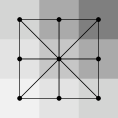
(b) simplicial grid whose nodes are located in the pixel centers

Figure 1: Image aligned simplicial grid construction as in [21].

Let $\mathcal{T}$ denote the set of cells and $\Gamma$ the set of oriented facets (i.e. edges as $d=2$) of the simplicial triangulation. For any cell $K\in\mathcal{T}$ let $P_{k}(K)$ be the space of polynomial functions on $K$ with total degree $k\in\mathbb{N}$. We define the finite subspaces $V_{h}\subseteq H^{1}(\Omega)^{m}=V$, $W_{h}^{*}\subseteq L^{2}(\Omega)\times L^{2}(\Omega)^{d\times m}\simeq W^{*}$, i.e. $W^{*}$ can be identified with $W=L^{2}(\Omega)\times L^{2}(\Omega)^{d\times m}$, and $Z_{h}\subseteq L^{2}(\Omega)$ as

$$V_{h} :=\{\mathbf{u}\in C(\Omega)^{m}:\mathbf{u}|_{K}\in P_{1}(K)^{m},K\in\mathcal{T}\},$$ (6)

$$W_{h}^{*} :=\{(p_{1},\mathbf{p}_{2})\in C(\Omega)\times L^{2}(\Omega)^{d\times m}:p_{1}|_{K}\in P_{1}(K),\mathbf{p}_{2}|_{K}\in P_{0}(K)^{d\times m},$$

$$\phantom{:=\{(p_{1},\mathbf{p}_{2})\in C(\Omega)\times L^{2}(\Omega)^{d\times m}:p_{1}|_{K}\in P_{1}(K),\mathbf{p}_{2}|_{K}\in P_{0}(K)}K\in\mathcal{T}\},$$

$$Z_{h} :=\{g\in C(\Omega):g|_{K}\in P_{1}(K),K\in\mathcal{T}\}.$$

As in [21] we do not discretize 1 directly but the optimality conditions 5 instead. In our discrete finite element setting this means that we search for solutions $\mathbf{p}_{h}=(p_{1_{h}},\mathbf{p}_{2,h})\in W_{h}^{*}$, $\mathbf{u}_{h}\in V_{h}$ which satisfy

$$0 =\Lambda^{*}\mathbf{p}_{h}-\alpha_{2}T^{*}g_{h}+B\mathbf{u}_{h},$$ (7)

$$0 =p_{1,h}\max\{\gamma_{1},|T\mathbf{u}_{h}-g_{h}|\}-\alpha_{1}(T\mathbf{u}_{h}-g_{h}), |p_{1,h}| \leq\alpha_{1},$$

$$0 =\mathbf{p}_{2,h}\max\{\gamma_{2},|\nabla\mathbf{u}_{h}|_{F}\}-\lambda\nabla\mathbf{u}_{h}, |\mathbf{p}_{2,h}|_{F} \leq\lambda,$$

where $g_{h}\in Z_{h}$ is a discrete version of the data $g$. We elaborate further in section 3.1 below on possibilities how to map image data onto the given grid. Note that the last two equations in 7 are enforced on vertices only. This is due to the fact, that the expression $|T\mathbf{u}_{h}-g_{h}|$ is not necessarily cell-wise linear, even though $T\mathbf{u}_{h}-g_{h}$ is.

Further we define: Let $F\in\Gamma$ be an oriented inner facet with adjacent cells $K_{1},K_{2}\in\mathcal{T}$ and $\mathbf{\varphi}\in L^{2}(K_{1}\cup K_{2})^{d\times m}$ with $\mathbf{\varphi}|_{K_{i}}\in C(K_{i})^{d\times m}$, $i\in\{1,2\}$, a square integrable function which allows continuous representations $\mathbf{\varphi}|_{K_{i}}$ on each cell $K_{i}$ individually. We then define the jump term $[\mathbf{\varphi}]_{F}\in C(F)^{d\times m}$ by $[\mathbf{\varphi}]_{F}(\mathbf{x}):=\mathbf{\varphi}|_{K_{1}}(\mathbf{x})-\mathbf{\varphi}|_{K_{2}}(\mathbf{x})$ and omit the index as in $[\mathbf{\varphi}]$ when the facet in question is clear. For outer facets only the term corresponding to the existing adjacent cell is considered. Note that $[\mathbf{\varphi}]_{F}$ is in general dependent on the orientation of $F$, while e.g. $[\mathbf{n}^{\top}\mathbf{\varphi}]_{F}$ for the oriented facet-normal $\mathbf{n}$ is not.

3.1 On Image Interpolation Methods

For aligned grids as in figure 1 image data $A\in[0,1]^{n_{1}\times n_{2}}$ is interpolated to a grid function $g_{h}\in Z_{h}$ by nodal sampling. This way, when resampling at pixel centers one receives the original image. For non-aligned grids, i.e. when pixel centers do not correspond to vertices of the grid, a mapping of the image $A$ to some grid function $g_{h}\in Z_{h}$ has to be computed. Choosing nodal sampling (e.g. of bilinearly interpolated image data) for this map can result in aliasing and is a well known undesired effect in image processing [13]. The Shannon-Whittaker sampling theorem provides ample conditions for correct equidistant sampling of bandwidth-limited functions [29, 13], namely to remove high-frequency contributions (e.g. by a linear smoothing filter) before sampling on a coarser grid. It is however unclear to us how to apply this to general unstructured sampling points.

We evaluate three projection schemes and then explore one alternative. Let $g\in C(\Omega)$ be the bilinear interpolation of the nodal image data $A$. For methods involving quadratures the quadrature over a cell $E\in\mathcal{T}$ is computed using a simple averaging quadrature on a Lagrange lattice of degree $\lceil\operatorname{diam}(E)\rceil$, i.e. we properly scale the number of quadrature points depending on the size of the cell (and thus the number of pixels it covers) to avoid aliasing effects.

The projection schemes are defined as follows:

1. nodal: Nodal interpolation, i.e. $g_{h}\in Z_{h}$ such that $g_{h}(\mathbf{x}):=g(\mathbf{x})$ at every mesh vertex $\mathbf{x}$.

2. l2lagrange: Standard $L^{2}$-projection, i.e. $g_{h}\in Z_{h}$ such that $\int_{\Omega}g_{h}\cdot\varphi\;\mathrm{d}\mathbf{x}=\int_{\Omega}g\cdot\varphi\;\mathrm{d}\mathbf{x}$ for all $\varphi\in Z_{h}$.

3. qilagrange: The general $L^{1}$-stable quasi-interpolation operator as proposed in [19], i.e. the continuous $g_{h}\in Z_{h}$ is given by setting its nodal degrees of freedom at each vertex to the arithmetic mean of the corresponding local degrees of freedom of a discontinuous interpolant $\widetilde{g}_{h}\in\widetilde{Z}_{h}:=\{f\in L^{\infty}(\Omega):f|_{K}\in P_{1}(K),K\in\mathcal{T}\}$, which is defined on each cell $K\in\mathcal{T}$ by its local nodal degrees of freedom $\sigma_{K,i}=\mathchoice{\tfrac{1}{|K|}}{\frac{1}{|K|}}{\frac{1}{|K|}}{\frac{1}{|K|}}\int_{K}g(\mathbf{x})\cdot\rho_{K,i}(\mathbf{x})\;\mathrm{d}\mathbf{x}$, $i=1,\dotsc,3$ where the test function $\rho_{K,i}$ in our case is given in barycentric coordinates $\lambda_{K}$ by $\rho_{K,i}(\lambda_{K})=12\lambda_{K,i}-3$. The reader may refer to [19] for details on the general construction.

4. l2pixel: Our proposed method, i.e. minimizing the sum of pointwise squared errors over all pixel coordinates: $\inf_{g_{h}\in Z_{h}}\sum_{\mathbf{x}\in\Omega\cap\mathbb{Z}^{2}}\tfrac{1}{2}\|g_{h}(\mathbf{x})-g(\mathbf{x})\|^{2}$.

Note that l2pixel may be interpreted as an $L^{2}$-projection with a cell-dependent averaging quadrature rule, adapted to the original image pixel locations.

Figure 2: Discrete input image for mesh interpolation comparison, $32\times 32$ pixels.

Figure 3: Interpolated finite element functions for varying mesh sizes and interpolation methods. Methods from left to right: nodal, l2lagrange, qilagrange, l2pixel. Number of mesh vertices in each dimension from top to bottom: 32, 16, 13.

Table 1: PSNR values (higher is better) of interpolated mesh functions from figure 3, sampled at image coordinates.

&nodall2lagrangeqilagrangel2pixel $32$$\infty$$55.826$$22.606$$327.597$ $16$$21.141$$22.020$$21.483$$23.106$ $13$$18.861$$19.650$$19.053$$19.981$

Table 2: SSIM values (higher is better) of interpolated mesh functions from figure 3, sampled at image coordinates.

&nodall2lagrangeqilagrangel2pixel $32$$1.000$$1.000$$0.978$$1.000$ $16$$0.939$$0.951$$0.948$$0.967$ $13$$0.893$$0.909$$0.901$$0.921$

We evaluate these schemes by interpolating the discrete image given in figure 2 onto $V_{h}$ for regular meshes of different sizes. In figure 3 we see the interpolated results as cellwise linear functions. We sample the interpolated functions on the original image grid $\Omega_{h}$ and quantify the error to the original image. In particular, sections 3.1 and 3.1 list the $\operatorname{PSNR}$, given for two scalar images $u,v:\Omega_{h}\to[0,1]$ by $\operatorname{PSNR}(u,v):=-10\log_{10}\big{(}\mathchoice{\tfrac{1}{|\Omega_{h}|}}{\frac{1}{|\Omega_{h}|}}{\frac{1}{|\Omega_{h}|}}{\frac{1}{|\Omega_{h}|}}\sum_{\mathbf{x}\in\Omega_{h}}(u(\mathbf{x})-v(\mathbf{x}))^{2}\big{)}$, and the structural similarity index $\operatorname{SSIM}$ as defined in [31]. Perhaps unsurprisingly, due to construction, l2pixel produces results closest to the original image for both metrics. We note that, theoretically, l2pixel in the finest mesh setting should provide exact results (i.e. infinite $\operatorname{PSNR}$) and the discrepancy is due to numerical imprecision.

It should be noted that while l2pixel seems to provide visually superior results, it does not necessarily preserve other quantities of the image, such as the total mass, which may be relevant for the image processing task in question. Further, it is not necessarily well-defined for meshes finer than the original image and in that case a regularization needs to be applied.

We conclude that, since digital images are usually given as an array of brightness values and the output of image processing algorithms is expected to be so too, working in unstructured finite element spaces comes with the drawback of information loss due to mesh interpolation. Apart from increased complexity, this may be considered a problem for applying unstructured adaptive finite element methods to image processing tasks in practice.

3.2 Residual A-Posteriori Error Estimator

In [23] an a-posteriori error estimate for a smooth functional, composed of an $L^{2}$-data term and a total variation term, was derived using residual-based methods for variational inequalities. We try to use a similar technique for our general setting to establish a suitable guiding criterion for adaptive spatial discretization. Our presentation avoids the variational inequality setting in [23] by making use of strong convexity, which seems to lead to a simpler presentation. Additionally, we consider both choices of items ($S$.i) and ($S$.ii), which requires different interpolation estimates depending on the corresponding coercivity of $a_{B}$ stated in item (A1).

Since the derivation requires local (cell-wise) adjoints $T^{*}$, we will make the following locality assumption on the operator $T$.

1. For almost every $\mathbf{x}\in\Omega$ there exists $f_{\mathbf{x}}:\mathbb{R}^{m}\to\mathbb{R}$ such that:

   $$(T\mathbf{u})(\mathbf{x})=f_{\mathbf{x}}(\mathbf{u}(\mathbf{x}))\qquad\forall\mathbf{u}\in V.$$ (8)

Note that item (A2) excludes global operators such as Fourier transforms. Implementing global operators in an unstructured finite element setting efficiently, however, is considered impractical at best because of the non-local access pattern and will therefore not be pursued here.

We recall $E:V\to\overline{\mathbb{R}}$ from 1 in the split form $E(\mathbf{u})=F(\mathbf{u})+G(\Lambda\mathbf{u})$, where $\Lambda=(T,\nabla):V\to W$ as in section 2.2 and $F:V\to\overline{\mathbb{R}}$, $G:W\to\overline{\mathbb{R}}$ are given by

$$F(\mathbf{u}) :=\tfrac{\alpha_{2}}{2}\|T\mathbf{u}-g\|_{L^{2}}^{2}+\tfrac{\beta}{2}\|S\mathbf{u}\|_{L^{2}}^{2},$$

$$G(\Lambda\mathbf{u}) :=\alpha_{1}\int_{\Omega}\varphi_{\gamma_{1}}(|T\mathbf{u}-g|)\;\mathrm{d}\mathbf{x}+\lambda\int_{\Omega}\varphi_{\gamma_{2}}(|\nabla\mathbf{u}|_{F})\;\mathrm{d}\mathbf{x}.$$

The optimality conditions in this setting, see [18, Remark III.4.2], are given by

$$-\Lambda^{*}p \in\partial F(\mathbf{u}),$$

$$p \in\partial G(\Lambda\mathbf{u}),$$

where we accounted for the sign change in the dual variable $p$ to be consistent with the formulation in 5. We assume for the moment that $\alpha_{1}=0$ and the discrete solution pair $\mathbf{u}_{h}\in V_{h}$, $\mathbf{p}_{h}\in W_{h}^{*}$ satisfies the corresponding discrete optimality conditions

$$-\Lambda^{*}\mathbf{p}_{h} \in\partial F_{h}(\mathbf{u}_{h}),$$ (9)

$$\mathbf{p}_{h} \in\partial G_{h}(\Lambda\mathbf{u}_{h}),$$

where for clarity we explicitly denoted with $F_{h}:V_{h}\to\overline{\mathbb{R}}$, $G_{h}:W_{h}\to\overline{\mathbb{R}}$ the restrictions of $F$, $G$ on the respective discrete spaces, since their subdifferentials differ from those of $F$ and $G$ respectively. Note that $W_{h}$ denotes the (pre-)dual space of $W_{h}^{*}$. One may obtain this system analogously to [21] by application of the Fenchel duality from [18, Remark III.4.2] on the corresponding discrete energy functional. Indeed, theorem 2.1 in general allows for $V$ and $W$ to be appropriate subspaces. This way existence of a discrete solution pair $\mathbf{u}_{h}\in V_{h}$, $\mathbf{p}_{h}\in W_{h}^{*}$ is ensured. Since $F$ is Fréchet-differentiable we see that

$$\langle\partial F(\mathbf{u}),\mathbf{v}\rangle_{V^{*},V} =\alpha_{2}\langle T\mathbf{u}-g,T\mathbf{v}\rangle_{L^{2}}+\beta\langle S\mathbf{u},S\mathbf{v}\rangle_{L^{2}}$$

$$=a_{B}(\mathbf{u},\mathbf{v})-l(\mathbf{v})$$

with $l(\mathbf{v}):=\alpha_{2}\langle T\mathbf{v},g\rangle_{L^{2}}$. Analogously $\langle\partial F_{h}(\mathbf{u}_{h}),\mathbf{v}_{h}\rangle_{V_{h}^{*},V_{h}}=a_{B}(\mathbf{u}_{h},\mathbf{v}_{h})-l(\mathbf{v}_{h})$ and from 9 we infer for all $\mathbf{v}_{h}\in V_{h}$:

$$-\langle\mathbf{p}_{h},\Lambda\mathbf{v}_{h}\rangle_{L^{2}}=a_{B}(\mathbf{u}_{h},\mathbf{v}_{h})-l(\mathbf{v}_{h}).$$ (10)

For $\partial G$ on the other hand we have the following non-obvious observation.

Lemma 3.1.

Let $\mathbf{p}_{h}=(p_{h,1},\mathbf{p}_{h,2})\in W_{h}^{*}$ satisfy 9. If $\alpha_{1}=0$ then

$$\mathbf{p}_{h}\in\partial G(\Lambda\mathbf{u}_{h}),$$

where $\mathbf{p}_{h}\in W_{h}^{*}\subseteq W^{*}$ is identified with an element of the dual space $(W^{*})^{*}=W$.

Proof.

Let $\mathbf{q}=(q_{1},\mathbf{q}_{2})\in\partial G(\Lambda\mathbf{u}_{h})$. Due to 5 and 9 we deduce $q_{1}=p_{h,1}=0$ since $\alpha_{1}=0$. From 5 we infer for $\mathbf{q}_{2}$, and analogously for $\mathbf{p}_{h,2}$, due to 9 that pointwise, whenever $\nabla\mathbf{u}_{h}\neq 0$, we have

$$\mathbf{q}_{2}=\mathchoice{\tfrac{\lambda\nabla\mathbf{u}_{h}}{\max\{\gamma_{2},|\nabla\mathbf{u}_{h}|_{F}\}}}{\frac{\lambda\nabla\mathbf{u}_{h}}{\max\{\gamma_{2},|\nabla\mathbf{u}_{h}|_{F}\}}}{\frac{\lambda\nabla\mathbf{u}_{h}}{\max\{\gamma_{2},|\nabla\mathbf{u}_{h}|_{F}\}}}{\frac{\lambda\nabla\mathbf{u}_{h}}{\max\{\gamma_{2},|\nabla\mathbf{u}_{h}|_{F}\}}}=\mathbf{p}_{h,2}.$$

Therefore $\mathbf{q}_{2}$ is piecewise constant whenever $\nabla\mathbf{u}_{h}\neq 0$. Further both $\mathbf{q}_{2}$ and $\mathbf{p}_{h,2}$ are bounded pointwise by $|\mathbf{q}_{2}|_{F}\leq\lambda$ and $|\mathbf{p}_{h,2}|_{F}\leq\lambda$. On cells where $\nabla\mathbf{u}_{h}=0$ holds, $\mathbf{q}_{2}$ may assume any value bounded by $|\mathbf{q}_{2}|_{F}\leq\lambda$. Since this holds true for $\mathbf{p}_{h,2}$ in particular, one may choose $\mathbf{q}:=(0,\mathbf{p}_{h,2})\in\partial G(\Lambda\mathbf{u}_{h})$. ∎

We note that for $\alpha_{1}>0$ the optimality conditions 9 might not be valid for $\mathbf{p}_{h}\in W_{h}^{*}$ due to the presence of the operator $T$. A possibility to circumvent this shortcoming might be to enlarge the space $W_{h}^{*}$ to $\{(p_{1},\mathbf{p}_{2})\in L^{2}(\Omega)\times L^{2}(\Omega)^{d\times m}:p_{1}|_{K}\in P_{1}(K),\mathbf{p}_{2}|_{K}\in P_{0}(K)^{d\times m},K\in\mathcal{T}\}$. However, even in such a new setting lemma 3.1 would not necessarily hold true for $\alpha_{1}>0$, as $\partial G(\Lambda\mathbf{u}_{h})=\alpha_{1}\tfrac{T\mathbf{u}_{h}-g}{\max\{\gamma_{1},|T\mathbf{u}_{h}-g|\}}$ does not need to be piecewise linear, even if $\mathbf{u}_{h}$ is. We will continue the derivation nevertheless, noting that theoretical justification is lacking for $\alpha_{1}>0$. That is in the sequel we assume that

$$\mathbf{p}_{h}\in\partial G(\Lambda\mathbf{u}_{h}).$$ (11)

With these observations we are ready to estimate the error $\|\mathbf{u}_{h}-\mathbf{u}\|_{B}$. Denote $\mathbf{e}_{h}:=\mathbf{u}_{h}-\mathbf{u}\in V$ and bound using lemma 2.2:

$$\tfrac{1}{2}\|\mathbf{u}_{h}-\mathbf{u}\|_{B}^{2} \leq E(\mathbf{u}_{h})-E(\mathbf{u})$$

$$=F(\mathbf{u}_{h})-F(\mathbf{u})+G(\Lambda\mathbf{u}_{h})-G(\Lambda\mathbf{u})$$

$$\leq\langle\partial F(\mathbf{u}_{h}),\mathbf{e}_{h}\rangle_{V^{*},V}+\langle\partial G(\Lambda\mathbf{u}_{h}),\Lambda\mathbf{e}_{h}\rangle_{L^{2}}$$

$$=a_{B}(\mathbf{u}_{h},\mathbf{e}_{h})-l(\mathbf{e}_{h})+\langle\partial G(\Lambda\mathbf{u}_{h}),\Lambda\mathbf{e}_{h}\rangle_{L^{2}}.$$

Depending on $S$, we will now further bound the error $\tfrac{1}{2}\|\mathbf{u}_{h}-\mathbf{u}\|_{B}^{2}$.

Item ($S$.ii): the Case ${S=\nabla}$

We will make use of the fact that $a_{B}$ is coercive on $V$, see item (A1), to derive an estimate on the error $\|\mathbf{e}_{h}\|_{H^{1}(\Omega)^{m}}$.

Due to 11 and the discrete optimality condition 10 we have for any bounded linear operator $I_{h}:V\to V_{h}$:

$$\tfrac{1}{2}\|\mathbf{u}_{h}-\mathbf{u}\|_{B}^{2} \leq a_{B}(\mathbf{u}_{h},\mathbf{e}_{h})-l(\mathbf{e}_{h})+\langle\mathbf{p}_{h},\Lambda\mathbf{e}_{h}\rangle_{L^{2}}$$ (12)

$$=a_{B}(\mathbf{u}_{h},\mathbf{e}_{h}-I_{h}\mathbf{e}_{h})-l(\mathbf{e}_{h}-I_{h}\mathbf{e}_{h})+\langle\mathbf{p}_{h},\Lambda(\mathbf{e}_{h}-I_{h}\mathbf{e}_{h})\rangle_{L^{2}}$$

$$=\langle\alpha_{2}(T\mathbf{u}_{h}-g)+p_{h,1},T(\mathbf{e}_{h}-I_{h}\mathbf{e}_{h})\rangle_{L^{2}}$$

$$\qquad+\langle\beta S\mathbf{u}_{h},S(\mathbf{e}_{h}-I_{h}\mathbf{e}_{h})\rangle_{L^{2}}+\langle\mathbf{p}_{h,2},\nabla(\mathbf{e}_{h}-I_{h}\mathbf{e}_{h})\rangle_{L^{2}}.$$

Actually we choose $I_{h}:V\to V_{h}$ to be a quasi-interpolation operator which satisfies the interpolation estimates [30, Proposition 1.3] [1, Theorem 1.7]:

$$\|\mathbf{v}-I_{h}\mathbf{v}\|_{L^{2}(K)} \leq c_{1}h_{K}\|\nabla\mathbf{v}\|_{L^{2}(\omega_{K})},$$ (13)

$$\|\mathbf{v}-I_{h}\mathbf{v}\|_{L^{2}(F)} \leq c_{2}h_{F}^{\mathchoice{\tfrac{1}{2}}{\frac{1}{2}}{\frac{1}{2}}{\frac{1}{2}}}\|\nabla\mathbf{v}\|_{L^{2}(\omega_{F})},$$ (14)

where $c_{1},c_{2}>0$, $\omega_{K}$, $\omega_{F}$ denote the union of triangles which share a common vertex with the cell $K$ or the facet $F$ respectively and $h_{K}$, $h_{F}$ denote the diameter of $K$ and $F$ respectively.

Utilizing Green’s formula, see e.g. [26, Proposition 2.4], in 12 yields

$$\tfrac{1}{2} \|\mathbf{u}_{h}-\mathbf{u}\|_{B}^{2}\leq\big{\langle}\alpha_{2}(T\mathbf{u}_{h}-g)+p_{h,1},T(\mathbf{e}_{h}-I_{h}\mathbf{e}_{h})\big{\rangle}_{L^{2}}$$

$$\phantom{\|\mathbf{u}_{h}-\mathbf{u}\|_{B}^{2}\leq}+\big{\langle}\beta\nabla\mathbf{u}_{h}+\mathbf{p}_{h,2},\nabla(\mathbf{e}_{h}-I_{h}\mathbf{e}_{h})\big{\rangle}_{L^{2}}$$

$$=\sum_{K\in\mathcal{T}}\bigg{(}\Big{\langle}\alpha_{2}T^{*}(T\mathbf{u}_{h}-g)+T^{*}p_{h,1}-\beta\operatorname{\Delta}\mathbf{u}_{h}-\operatorname{div}\mathbf{p}_{h,2},\mathbf{e}_{h}-I_{h}\mathbf{e}_{h}\Big{\rangle}_{L^{2}(K)^{m}}$$

$$\qquad\qquad+\Big{\langle}\mathbf{n}^{\top}(\beta\nabla\mathbf{u}_{h}+\mathbf{p}_{h,2}),\mathbf{e}_{h}-I_{h}\mathbf{e}_{h}\Big{\rangle}_{L^{2}(\partial K)^{m}}\bigg{)},$$

where we used locality of $T$ from item (A2). Denoting $\mathbf{\xi}:=\alpha_{2}T^{*}(T\mathbf{u}_{h}-g)+T^{*}p_{h,1}-\beta\operatorname{\Delta}\mathbf{u}_{h}-\operatorname{div}\mathbf{p}_{h,2}\in L^{2}(\Omega)^{m}$ and $\mathbf{\zeta}:=\beta\nabla\mathbf{u}_{h}+\mathbf{p}_{h,2}\in L^{2}(\Omega)^{d\times m}$ we obtain using interpolation estimates 13 and 14:

$$\tfrac{1}{2}\|\mathbf{u}_{h}-\mathbf{u}\|_{B}^{2} \leq\sum_{K\in\mathcal{T}}\Big{(}\langle\xi,\mathbf{e}_{h}-I\mathbf{e}_{h}\rangle_{L^{2}(K)^{m}}+\langle\mathbf{n}^{\top}\zeta,\mathbf{e}_{h}-I\mathbf{e}_{h}\rangle_{L^{2}(\partial K)^{m}}\Big{)}$$

$$=\sum_{K\in\mathcal{T}}\langle\xi,\mathbf{e}_{h}-I\mathbf{e}_{h}\rangle_{L^{2}(K)^{m}}+\sum_{F\in\Gamma}\langle[\mathbf{n}^{\top}\zeta],\mathbf{e}_{h}-I\mathbf{e}_{h}\rangle_{L^{2}(F)^{m}}$$

$$\leq\max\{c_{1},c_{2}\}\Big{(}\sum_{K\in\mathcal{T}}\|\nabla\mathbf{e}_{h}\|_{L^{2}(\omega_{K})^{d\times m}}h_{K}\|\xi\|_{L^{2}(K)^{m}}$$

$$\qquad\qquad\qquad\quad+\sum_{F\in\Gamma}\|\nabla\mathbf{e}_{h}\|_{L^{2}(\omega_{F})^{d\times m}}h_{F}^{\mathchoice{\tfrac{1}{2}}{\frac{1}{2}}{\frac{1}{2}}{\frac{1}{2}}}\|[\mathbf{n}^{\top}\zeta]\|_{L^{2}(F)^{m}}\Big{)}$$

$$\leq\max\{c_{1},c_{2}\}\Big{(}\sum_{K\in\mathcal{T}}\|\nabla\mathbf{e}_{h}\|_{L^{2}(\omega_{K})^{d\times m}}^{2}+\sum_{F\in\Gamma}\|\nabla\mathbf{e}_{h}\|_{L^{2}(\omega_{F})^{d\times m}}^{2}\Big{)}^{\mathchoice{\tfrac{1}{2}}{\frac{1}{2}}{\frac{1}{2}}{\frac{1}{2}}}$$

$$\qquad\qquad\qquad\quad\Big{(}\sum_{K\in\mathcal{T}}h_{K}^{2}\|\xi\|_{L^{2}(K)^{m}}^{2}+\sum_{F\in\Gamma}h_{F}\|[\mathbf{n}^{\top}\zeta]\|_{L^{2}(F)^{m}}^{2}\Big{)}^{\mathchoice{\tfrac{1}{2}}{\frac{1}{2}}{\frac{1}{2}}{\frac{1}{2}}}.$$

Let $B(K)$ be the set of facets of $K$ belonging to $\partial\Omega$ and $I(K)$ all other facets of $K$. Realizing that $\omega_{F}\subseteq\omega_{K}$ for all to $F$ adjacent cells $K$ and having at most one boundary facet at each cell we may bound

$$\begin{split}\sum_{F\in\Gamma}\|&\nabla\mathbf{e}_{h}\|_{L^{2}(\omega_{F})^{d\times m}}^{2}\\ &=\sum_{K\in\mathcal{T}}\left(\sum_{F\in B(K)}\|\nabla\mathbf{e}_{h}\|_{L^{2}(\omega_{F})^{d\times m}}^{2}+\mathchoice{\tfrac{1}{2}}{\frac{1}{2}}{\frac{1}{2}}{\frac{1}{2}}\sum_{F\in I(K)}\|\nabla\mathbf{e}_{h}\|_{L^{2}(\omega_{F})^{d\times m}}^{2}\right)\\ &\leq\sum_{K\in\mathcal{T}}\left(\sum_{F\in B(K)}\|\nabla\mathbf{e}_{h}\|_{L^{2}(\omega_{K})^{d\times m}}^{2}+\mathchoice{\tfrac{1}{2}}{\frac{1}{2}}{\frac{1}{2}}{\frac{1}{2}}\sum_{F\in I(K)}\|\nabla\mathbf{e}_{h}\|_{L^{2}(\omega_{K})^{d\times m}}^{2}\right)\\ &\leq 2\sum_{K\in\mathcal{T}}\|\nabla\mathbf{e}_{h}\|_{L^{2}(\omega_{K})^{d\times m}}^{2}\leq 2c_{\mathcal{T}}^{2}\|\nabla\mathbf{e}_{h}\|_{L^{2}(\Omega)^{d\times m}}^{2},\end{split}$$ (15)

where $c_{\mathcal{T}}$ denotes the shape regularity constant of the mesh independent of the mesh size. We thus arrive at

$$\tfrac{1}{2}\|\mathbf{u}_{h}-\mathbf{u}\|_{B}^{2}$$

$$\quad\leq\max\{c_{1},c_{2}\}\Big{(}3\sum_{K\in\mathcal{T}}\|\nabla\mathbf{e}_{h}\|_{L^{2}(\omega_{K})^{d\times m}}^{2}\Big{)}^{\mathchoice{\tfrac{1}{2}}{\frac{1}{2}}{\frac{1}{2}}{\frac{1}{2}}}\Big{(}\sum_{K\in\mathcal{T}}h_{K}^{2}\|\xi\|_{L^{2}(K)^{m}}^{2}$$

$$\phantom{\hskip 213.39566pt}+\sum_{F\in\Gamma}h_{F}\|[\mathbf{n}^{\top}\zeta]\|_{L^{2}(F)^{m}}^{2}\Big{)}^{\mathchoice{\tfrac{1}{2}}{\frac{1}{2}}{\frac{1}{2}}{\frac{1}{2}}}$$

$$\quad\leq\sqrt{3}\max\{c_{1},c_{2}\}c_{\mathcal{T}}\|\nabla\mathbf{e}_{h}\|_{L^{2}(\Omega)^{d\times m}}\Big{(}\sum_{K\in\mathcal{T}}h_{K}^{2}\|\xi\|_{L^{2}(K)^{m}}^{2}$$

$$\phantom{\hskip 213.39566pt}+\sum_{F\in\Gamma}h_{F}\|[\mathbf{n}^{\top}\zeta]\|_{L^{2}(F)^{m}}^{2}\Big{)}^{\mathchoice{\tfrac{1}{2}}{\frac{1}{2}}{\frac{1}{2}}{\frac{1}{2}}}$$

$$\quad\leq\sqrt{3}\max\{c_{1},c_{2}\}c_{\mathcal{T}}\|\mathbf{e}_{h}\|_{H^{1}(\Omega)^{m}}\Big{(}\sum_{K\in\mathcal{T}}h_{K}^{2}\|\xi\|_{L^{2}(K)^{m}}^{2}$$

$$\phantom{\hskip 213.39566pt}+\sum_{F\in\Gamma}h_{F}\|[\mathbf{n}^{\top}\zeta]\|_{L^{2}(F)^{m}}^{2}\Big{)}^{\mathchoice{\tfrac{1}{2}}{\frac{1}{2}}{\frac{1}{2}}{\frac{1}{2}}}.$$

Together with coercivity $\|\mathbf{v}\|_{B}^{2}=a_{B}(\mathbf{v},\mathbf{v})\geq c_{B}\|\mathbf{v}\|_{V}^{2}=c_{B}\|\mathbf{v}\|_{H^{1}(\Omega)^{m}}^{2}$ from item (A1) we arrive at an a-posteriori error bound

$$\|\mathbf{u}_{h} -\mathbf{u}\|_{H^{1}(\Omega)^{m}}^{2}$$

$$\leq C\bigg{(}\sum_{K\in\mathcal{T}}h_{K}^{2}\|\alpha_{2}T^{*}(T\mathbf{u}_{h}-g)+T^{*}p_{h,1}-\beta\operatorname{\Delta}\mathbf{u}_{h}-\operatorname{div}\mathbf{p}_{h,2}\|_{L^{2}(K)^{m}}^{2}$$

$$\qquad\qquad+\sum_{F\in\Gamma}h_{F}\|[\mathbf{n}^{\top}(\beta\nabla\mathbf{u}_{h}+\mathbf{p}_{h,2})]\|_{L^{2}(F)^{m}}^{2}\bigg{)}$$

with constant $C:=\mathchoice{\tfrac{12}{c_{B}}}{\frac{12}{c_{B}}}{\frac{12}{c_{B}}}{\frac{12}{c_{B}}}\max\{c_{1}^{2},c_{2}^{2}\}c_{\mathcal{T}}^{2}$.

Item ($S$.i): the case ${S=I}$

Using the fact that $a_{B}$ is coercive in this setting with respect to $L^{2}$, see item (A1), we derive an estimate for the error $\|\mathbf{e}_{h}\|_{L^{2}(\Omega)^{m}}$.

Let $I_{h}:L^{2}(\Omega)^{m}\to V_{h}$ be a bounded and linear quasi-interpolation operator satisfying the interpolation estimate [1, Theorem 1.7]:

$$\|\mathbf{v}-I_{h}\mathbf{v}\|_{L^{2}(F)}\leq c_{3}h_{F}^{-\mathchoice{\tfrac{1}{2}}{\frac{1}{2}}{\frac{1}{2}}{\frac{1}{2}}}\|\mathbf{v}\|_{L^{2}(\omega_{F})},$$ (16)

where $c_{3}>0$. Then, as above in item ($S$.ii), cf. 12, we obtain from 11 and the discrete optimality condition 10 that we have

$$\tfrac{1}{2}\|\mathbf{u}_{h}-\mathbf{u}\|_{B}^{2} =\langle\alpha_{2}(T\mathbf{u}_{h}-g)+p_{h,1},T(\mathbf{e}_{h}-I_{h}\mathbf{e}_{h})\rangle_{L^{2}}$$ (17)

$$\qquad+\langle\beta S\mathbf{u}_{h},S(\mathbf{e}_{h}-I_{h}\mathbf{e}_{h})\rangle_{L^{2}}+\langle\mathbf{p}_{h,2},\nabla(\mathbf{e}_{h}-I_{h}\mathbf{e}_{h})\rangle_{L^{2}}.$$

Applying Green’s formula to 17 yields the estimate

$$\tfrac{1}{2}a_{B}( \mathbf{e}_{h},\mathbf{e}_{h})\leq\langle\alpha_{2}T^{*}(T\mathbf{u}_{h}-g)+T^{*}p_{h,1}+\beta\mathbf{u}_{h},\mathbf{e}_{h}-I_{h}\mathbf{e}_{h}\rangle_{L^{2}}$$

$$\phantom{\mathbf{e}_{h},\mathbf{e}_{h})\leq\langle}+\langle\mathbf{p}_{h,2},\nabla(\mathbf{e}_{h}-I_{h}\mathbf{e}_{h})\rangle_{L^{2}}$$

$$\leq\sum_{K\in\mathcal{T}}\bigg{(}\Big{\langle}\alpha_{2}T^{*}(T\mathbf{u}_{h}-g)+T^{*}p_{h,1}+\beta\mathbf{u}_{h}-\operatorname{div}\mathbf{p}_{h,2},\mathbf{e}_{h}-I_{h}\mathbf{e}_{h}\Big{\rangle}_{L^{2}(K)^{m}}$$

$$\phantom{\mathbf{e}_{h},\mathbf{e}_{h})\leq\langle}+\Big{\langle}\mathbf{n}^{\top}\mathbf{p}_{h,2},\mathbf{e}_{h}-I_{h}\mathbf{e}_{h}\Big{\rangle}_{L^{2}(\partial K)^{m}}\bigg{)}.$$

Denoting $\xi:=\alpha_{2}T^{*}(T\mathbf{u}_{h}-g)+T^{*}p_{h,1}+\beta\mathbf{u}_{h}-\operatorname{div}\mathbf{p}_{h,2}$ and $\zeta:=\mathbf{n}^{\top}\mathbf{p}_{h,2}$ for brevity one continues to derive using 16, Cauchy-Schwarz inequality and 15:

$$\tfrac{1}{2} a_{B}(\mathbf{e}_{h},\mathbf{e}_{h})$$

$$\leq\sum_{K\in\mathcal{T}}\|\xi\|_{L^{2}(K)^{m}}\|\mathbf{e}_{h}-I_{h}\mathbf{e}_{h}\|_{L^{2}(K)^{m}}+\sum_{F\in\Gamma}\|[\zeta]\|_{L^{2}(F)^{m}}\|\mathbf{e}_{h}-I_{h}\mathbf{e}_{h}\|_{L^{2}(F)^{m}}$$

$$\stackrel{{\scriptstyle[}}{{]}}{\lx@cref{refnum}{eq:interpolation-estimate-3}}{\leq}\sum_{K\in\mathcal{T}}\|\xi\|_{L^{2}(K)^{m}}\|\mathbf{e}_{h}-I_{h}\mathbf{e}_{h}\|_{L^{2}(K)^{m}}+\sum_{F\in\Gamma}\|[\zeta]\|_{L^{2}(F)^{m}}h_{F}^{-1/2}c_{3}\|\mathbf{e}_{h}\|_{L^{2}(\omega_{F})^{m}}$$

$$\stackrel{{\scriptstyle[}}{{]}}{\begin{subarray}{c}\text{C.-S.}\\ \text{ineq.}\end{subarray}}{\leq}\left(\sum_{K\in\mathcal{T}}\|\mathbf{e}_{h}-I_{h}\mathbf{e}_{h}\|_{L^{2}(K)^{m}}^{2}+\sum_{F\in\Gamma}c_{3}^{2}\|\mathbf{e}_{h}\|_{L^{2}(\omega_{F})^{m}}^{2}\right)^{\mathchoice{\tfrac{1}{2}}{\frac{1}{2}}{\frac{1}{2}}{\frac{1}{2}}}\Bigg{(}\sum_{K\in\mathcal{T}}\|\xi\|_{L^{2}(K)^{m}}^{2}$$

$$\phantom{\hskip 227.62204pt}+\sum_{F\in\Gamma}h_{F}^{-1}\|[\zeta]\|_{L^{2}(F)^{m}}^{2}\Bigg{)}^{\mathchoice{\tfrac{1}{2}}{\frac{1}{2}}{\frac{1}{2}}{\frac{1}{2}}}$$

$$\leq\left(\sum_{K\in\mathcal{T}}\tilde{c}\|\mathbf{e}_{h}\|_{L^{2}(K)^{m}}^{2}+\sum_{F\in\Gamma}c_{3}^{2}\|\mathbf{e}_{h}\|_{L^{2}(\omega_{F})^{m}}^{2}\right)^{\mathchoice{\tfrac{1}{2}}{\frac{1}{2}}{\frac{1}{2}}{\frac{1}{2}}}\Bigg{(}\sum_{K\in\mathcal{T}}\|\xi\|_{L^{2}(K)^{m}}^{2}$$

$$\phantom{\hskip 227.62204pt}+\sum_{F\in\Gamma}h_{F}^{-1}\|[\zeta]\|_{L^{2}(F)^{m}}^{2}\Bigg{)}^{\mathchoice{\tfrac{1}{2}}{\frac{1}{2}}{\frac{1}{2}}{\frac{1}{2}}}$$

$$\stackrel{{\scriptstyle[}}{{]}}{\lx@cref{refnum}{Eq:cell_inequ}}{\leq}\left(\sum_{K\in\mathcal{T}}\tilde{c}\|\mathbf{e}_{h}\|_{L^{2}(\omega_{K})^{m}}^{2}+2c_{3}^{2}\|\mathbf{e}_{h}\|_{L^{2}(\omega_{K})^{m}}^{2}\right)^{\mathchoice{\tfrac{1}{2}}{\frac{1}{2}}{\frac{1}{2}}{\frac{1}{2}}}\Bigg{(}\sum_{K\in\mathcal{T}}\|\xi\|_{L^{2}(K)^{m}}^{2}$$

$$\phantom{\hskip 227.62204pt}+\sum_{F\in\Gamma}h_{F}^{-1}\|[\zeta]\|_{L^{2}(F)^{m}}^{2}\Bigg{)}^{\mathchoice{\tfrac{1}{2}}{\frac{1}{2}}{\frac{1}{2}}{\frac{1}{2}}}$$

$$\stackrel{{\scriptstyle[}}{{]}}{\lx@cref{refnum}{Eq:cell_inequ}}{\leq}\left(\tilde{c}+2c_{3}^{2}\right)^{\mathchoice{\tfrac{1}{2}}{\frac{1}{2}}{\frac{1}{2}}{\frac{1}{2}}}c_{\mathcal{T}}\|\mathbf{e}_{h}\|_{L^{2}(\Omega)^{m}}\left(\sum_{K\in\mathcal{T}}\|\xi\|_{L^{2}(K)^{m}}^{2}+\sum_{F\in\Gamma}h_{F}^{-1}\|[\zeta]\|_{L^{2}(F)^{m}}^{2}\right)^{\mathchoice{\tfrac{1}{2}}{\frac{1}{2}}{\frac{1}{2}}{\frac{1}{2}}},$$

where $\tilde{c}>0$. Together with the $L^{2}$-coercivity of $a_{B}$ from item (A1) we arrive at

$$\|\mathbf{u}_{h}-\mathbf{u}\|_{L^{2}(\Omega)^{m}}^{2} \leq C\bigg{(}\sum_{K\in\mathcal{T}}\|\alpha_{2}T^{*}(T\mathbf{u}_{h}-g)+T^{*}p_{h,1}+\beta\mathbf{u}_{h}-\operatorname{div}\mathbf{p}_{h,2}\|_{L^{2}(K)^{m}}^{2}$$

$$\qquad\qquad+\sum_{F\in\Gamma}h_{F}^{-1}\|[\mathbf{n}^{\top}\mathbf{p}_{h,2}]\|_{L^{2}(F)^{m}}^{2}\bigg{)}$$

for some constant $C>0$.

Error Indicators

For a cell $K\in\mathcal{T}$ we define our local error indicators as follows

$$\eta_{2,K}^{2}:=\tilde{\eta}_{2,K}^{2}+\sum_{\begin{subarray}{c}F\in\Gamma\\ F\cap K\neq\emptyset\end{subarray}}\tilde{\eta}_{2,F}^{2},$$ (18)

where $\tilde{\eta}_{2,K}$ and $\tilde{\eta}_{2,F}$ are chosen as follows. For item ($S$.ii) and $S=\nabla$ we set

$$\tilde{\eta}_{2,K}^{2} :=h_{K}^{2}\big{\|}\alpha_{2}T^{*}(T\mathbf{u}_{h}-g)+T^{*}p_{h,1}-\beta\operatorname{\Delta}\mathbf{u}_{h}-\operatorname{div}\mathbf{p}_{h,2}\big{\|}^{2}_{L^{2}(K)^{m}},$$ (19)

$$\tilde{\eta}_{2,F}^{2} :=h_{F}\big{\|}[\mathbf{n}^{\top}(\beta\nabla\mathbf{u}_{h}+\mathbf{p}_{h,2})]\big{\|}^{2}_{L^{2}(F)^{m}},$$

where for piecewise linear $\mathbf{u}_{h}$ and piecewise constant $\mathbf{p}_{h,2}$ the terms $\operatorname{\Delta}\mathbf{u}_{h}$ and $\operatorname{div}\mathbf{p}_{h,2}$ in 19 vanish. For item ($S$.i) and $S=I$ we set

$$\tilde{\eta}_{2,K}^{2} :=\big{\|}\alpha_{2}T^{*}(T\mathbf{u}_{h}-g)+T^{*}p_{h,1}+\beta\mathbf{u}_{h}-\operatorname{div}\mathbf{p}_{h,2}\big{\|}_{L^{2}(K)^{m}}^{2},$$

$$\tilde{\eta}_{2,F}^{2} :=h_{F}^{-1}\big{\|}[\mathbf{n}^{\top}\mathbf{p}_{h,2}]\big{\|}_{L^{2}(F)^{m}}^{2}.$$

Note that the indicators are computable locally on each cell again because of item (A2). For item ($S$.i) with $S=I$ the facet indicator $\tilde{\eta}_{2,F}$ scales inversely with the diameter and is therefore not very useful in the context of adaptive refinement. This is due to $a_{B}$ only being $L^{2}$-coercive in that case, which limits our choice of interpolation estimates and it is unclear to us whether this result can be improved. Showing efficiency of these estimators may be considered in future work and is expected to work out in a similar way as in [23].

3.3 Refinement Strategy

For refinement we bisect triangles using the newest-vertex strategy [27], i.e. the bisection edge is chosen to be opposite of the vertex which was inserted last. In an adaptive refinement setting we mark cells for refinement using the greedy Dörfler marking strategy [27] with $\theta_{\text{mark}}=0.5$, i.e. given error indicators in descending order $(\eta_{K_{n}})_{1\leq n\leq|\mathcal{T}|}$ for triangles $K_{n}\in\mathcal{T}$ we refine the first $n_{\text{mark}}\in\mathbb{N}$ triangles that satisfy

$$\sum_{n=1}^{n_{\text{mark}}}\eta_{K_{n}}\geq\theta_{\text{mark}}\sum_{n=1}^{|\mathcal{T}|}\eta_{K_{n}}.$$

3.4 Adaptive Finite Element Algorithm

Our generic adaptive finite element algorithm for solving 1 is presented in algorithm 1.

Algorithm 1 (AFEM for 1).

1. Choose an initial grid $\mathcal{T}$.

2. Find a finite element solution $\mathbf{u}_{h}$ of 1 on $\mathcal{T}$, e.g. by [21, Algorithm 1].

3. Compute on each cell the local indicator given by 18.

4. Stop if a certain termination criterion holds (e.g. the a-posteriori error estimators are sufficiently small), or continue with next step.

5. Determine $\mathcal{R}_{h}$, the set of cells to be refined, by using the greedy Dörfler strategy as described in section 3.3.

6. Refine the cells $K\in\mathcal{R}_{h}$ by utilizing newest-vertex bisection and set $\mathcal{T}$ to be the new grid.

7. Project the image data onto $\mathcal{T}$ (e.g. by l2lagrange or l2pixel) and continue with step 2.).

4 Application: Motion Estimation

We apply the adaptive finite element algorithm, see algorithm 1, developed for our model 1 to estimate motion in image sequences. For finding a finite element solution $\mathbf{u}_{h}$ in step 2 of algorithm 1 we utilize the primal-dual semi-smooth Newton method of [21].

Motion estimation is the problem of numerically computing the apparent motion field in a sequence of images. Following the discussion in [21] the motion field $\mathbf{u}$ of two (smooth) images $f_{0}$, $f_{1}$ may be computed solving model 1 with

$$T\mathbf{u}:=\nabla f_{w}\cdot\mathbf{u},\qquad g:=\nabla f_{w}\cdot\mathbf{u}_{0}-(f_{w}-f_{0}),$$

where $f_{w}(\mathbf{x}):=f_{1}(\mathbf{x}+\mathbf{u}_{0}(\mathbf{x}))$ is a warped version of $f_{1}$ with $\mathbf{u}_{0}$ being some smooth initial guess and $\mathbf{x}\in\Omega$. To account for large displacements an optical flow warping algorithm is introduced [21, Algorithm 3].

We combine the warping technique from [21, Algorithm 3] with adaptive refinement leading to LABEL:alg:optflow_adapt.

Algorithm 2 (Optical flow algorithm with adaptive warping).

Parameters: warping threshold $\varepsilon_{\text{warp}}$, parameters for [21, Algorithm 1] Input: images $f_{0},f_{1}$, initial guess $\mathbf{u}_{0}$ Output: motion fields $(\mathbf{u}_{k})_{k}$

$f_{w,0}(\mathbf{x})=f_{1}(\mathbf{x}+\mathbf{u}_{0}(\mathbf{x}))$

for $k=1,2,\dotsc$ do

     find approximate discrete solution $\mathbf{u}_{k}$ to 1 using [21, Algorithm 1]

     $f_{w,k}(\mathbf{x})=f_{1}(\mathbf{x}+\mathbf{u}_{k}(\mathbf{x}))$

     if $\tfrac{\|f_{w,k-1}-f_{0}\|_{L^{2}}-\|f_{w,k}-f_{0}\|_{L^{2}}}{\|f_{w,k-1}-f_{0}\|_{L^{2}}}<\varepsilon_{\text{warp}}$ then

         refine mesh and reproject image data

     end if

end for

To approximately solve for $\mathbf{u}_{k}$ in LABEL:alg:optflow_adapt, we use our model 1 by choosing $T\mathbf{u}:=\nabla f_{w,k-1}\cdot\mathbf{u}$ and $g:=\nabla f_{w,k-1}\cdot\mathbf{u}_{k-1}-(f_{w,k-1}-f_{0})$ and utilize the primal-dual semi-smooth Newton method of [21]. Thereby we use the discrete space $Z_{h}$ for the images $f_{0}$, $f_{1}$, $f_{w,k}$, except for the warping step, in which $f_{w,k}(\mathbf{x})=f_{1}(\mathbf{x}+\mathbf{u}_{k}(\mathbf{x}))$ is carried out at original image resolution by evaluating $f_{1}$ using bicubic interpolation and in a second step projected (e.g. using l2lagrange or l2pixel) onto the current finite element space in order to capture more detailed displacement information. For $g$ we instead use a cellwise linear discontinuous space to capture the discontinuous component $\nabla f_{w,k-1}$.

Loosely speaking, LABEL:alg:optflow_adapt solves the linearized optical flow equation for $u_{k}$ and warps the input data by the computed flow field until it no longer improves on the data difference $f_{w,k}-f_{0}$, which indicates displacement. In that case, the mesh is refined using the indicators from 18 and the process repeats, now including more detailed image data.

We note, that this approach to adaptivity allows us to start off with a coarse mesh and refine cells only if deemed necessary by the error indicator. In that respect it is different from the only other adaptive finite element methods for optical flow we are aware of, see [10, 11], where the mesh is initialized at fine image resolution first and iteratively coarsened only after a costly computation of the flow field and a suitable metric for adaptivity on this fine mesh has been established.

Experiments

The implementation of the performed algorithms is done in the programming language Julia [12] and can be found at [20]. All evaluations were done on a notebook with a Intel Core i7-10875H CPU @ 2.30GHz and 32GB RAM.

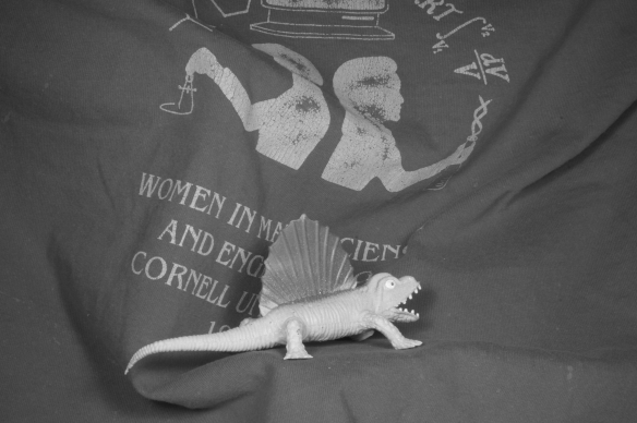
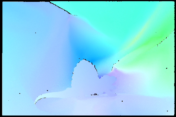
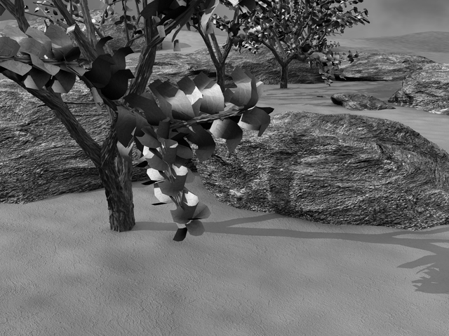
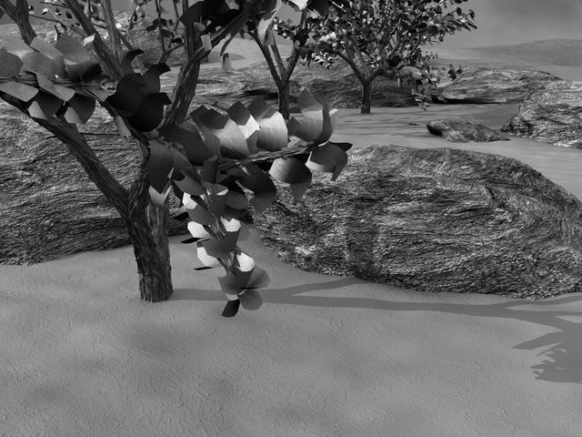
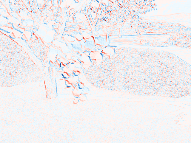
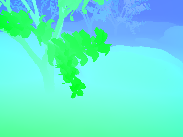
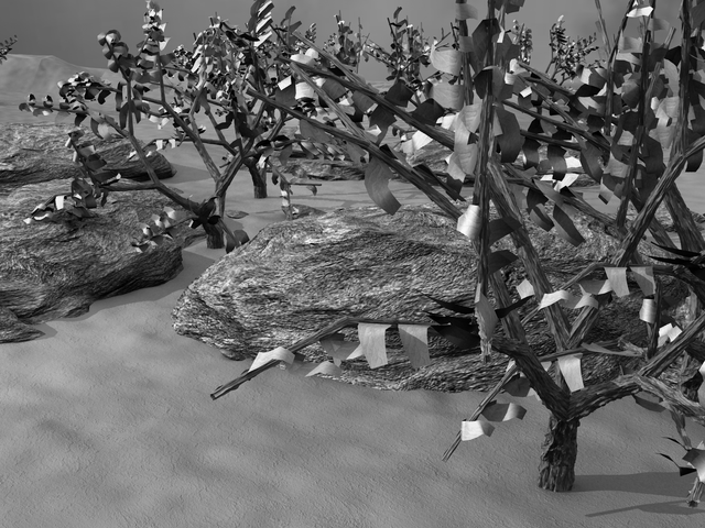
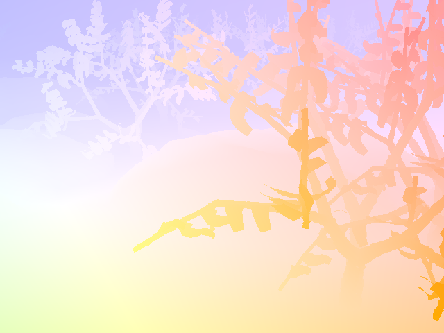
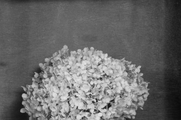
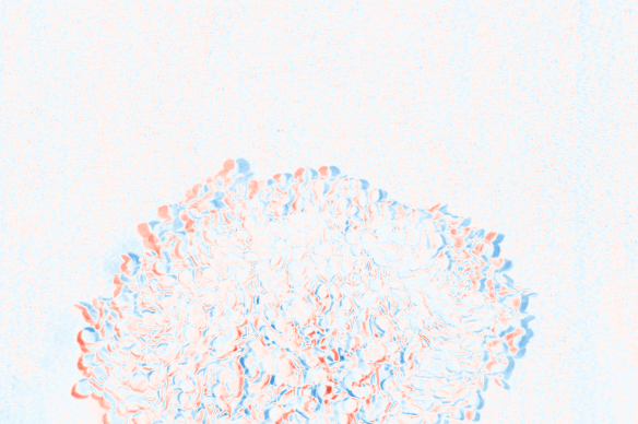
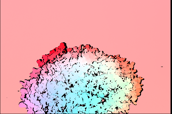
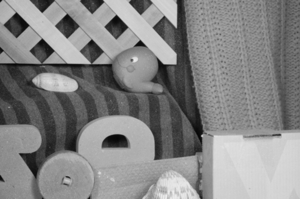
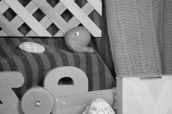
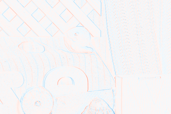
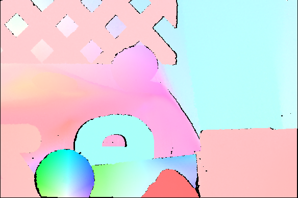
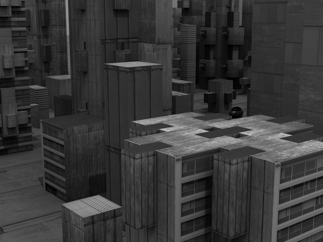
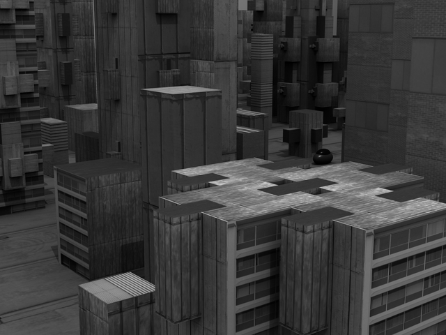
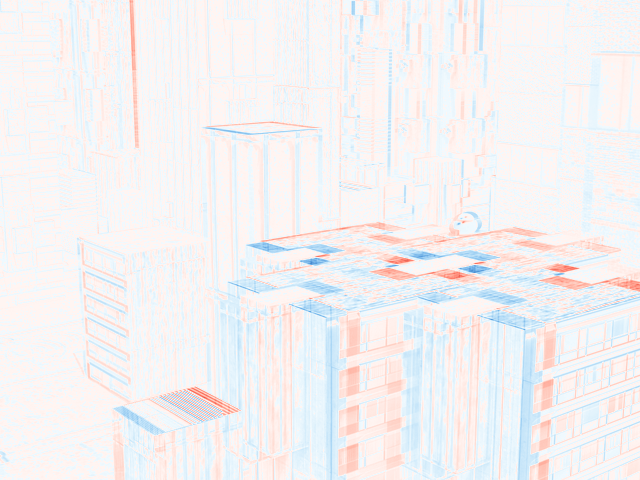
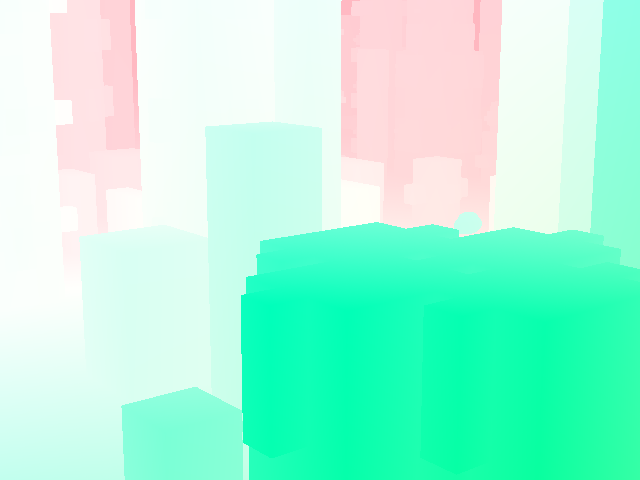
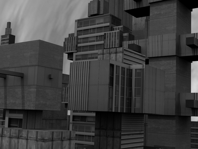
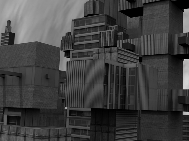
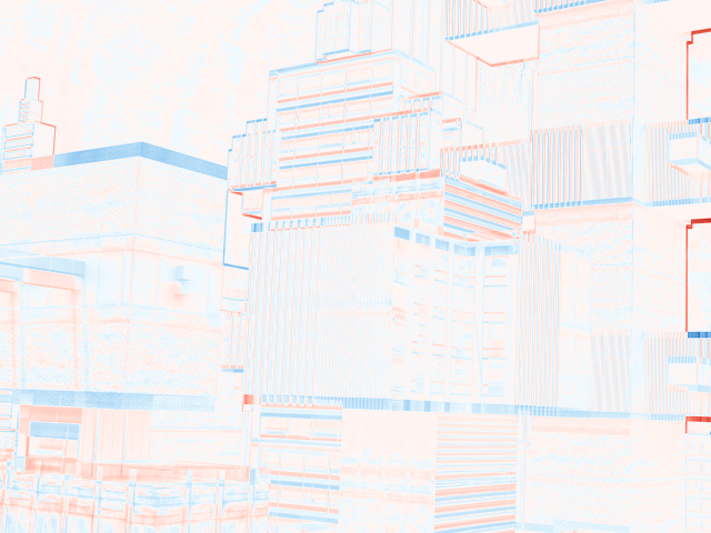
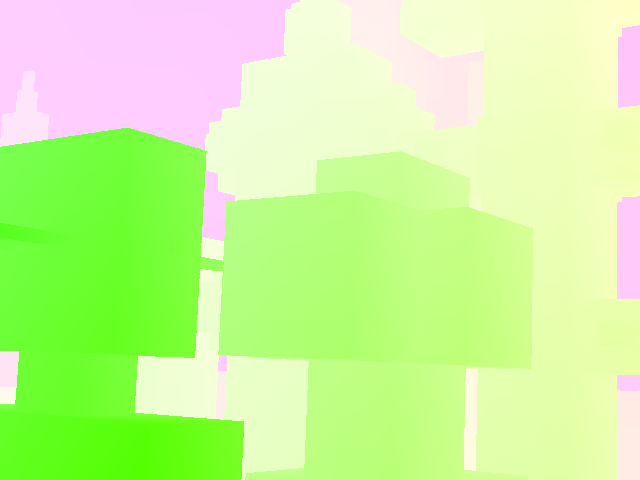
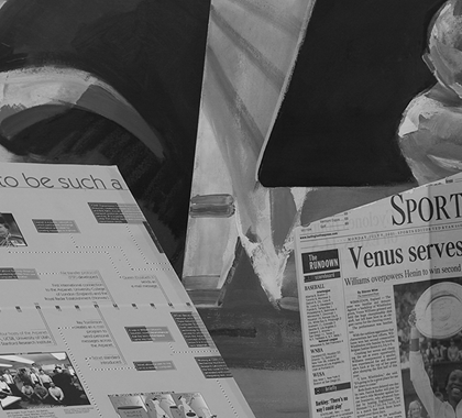
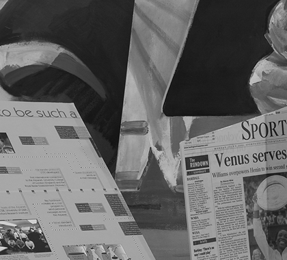
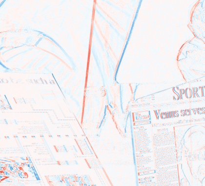
Figure 4: Middlebury Optical Flow Benchmark for $S=\nabla$: columns from left to right: $f_{0}$, $f_{1}$, image difference $f_{1}-f_{0}$, computed optical flow $\mathbf{u}$ using [21, Algorithm 3] without warping and with warping, computed optical flow $\mathbf{u}$ using LABEL:alg:optflow_adapt (adaptive warping), ground truth optical flow . Benchmarks from top to bottom: Dimetrodon, Grove2, Grove3, Hydrangea, RubberWhale, Urban2, Urban3, Venus.

& $0.41$ $0.37$ $0.13$ $0.12$ $83.96$ LABEL:alg:optflow_adapt (with l2-pixel) $0.42$ $0.38$ $0.14$ $0.12$ $74.62$

Grove2 [21, Algorithm 3] without warping $2.93$ $0.46$ $1.10$ $0.14$ $285.74$ [21, Algorithm 3] with warping $1.13$ $1.30$ $0.42$ $0.54$ $1{,}727.35$ LABEL:alg:optflow_adapt (with l2lagrange) $0.40$ $0.56$ $0.11$ $0.16$ $152.76$ LABEL:alg:optflow_adapt (with l2-pixel) $0.39$ $0.56$ $0.11$ $0.16$ $124.45$ Grove3 [21, Algorithm 3] without warping $3.69$ $2.33$ $1.01$ $0.32$ $312.74$ [21, Algorithm 3] with warping $1.93$ $2.11$ $0.26$ $0.29$ $1{,}628.13$ LABEL:alg:optflow_adapt (with l2lagrange) $1.12$ $1.50$ $0.16$ $0.29$ $168.02$ LABEL:alg:optflow_adapt (with l2-pixel) $1.10$ $1.49$ $0.16$ $0.29$ $176.56$ Hydrangea [21, Algorithm 3] without warping $3.33$ $1.22$ $0.91$ $0.23$ $222.65$ [21, Algorithm 3] with warping $0.22$ $0.52$ $0.04$ $0.10$ $1{,}396.16$ LABEL:alg:optflow_adapt (with l2lagrange) $0.58$ $0.47$ $0.08$ $0.11$ $106.36$ LABEL:alg:optflow_adapt (with l2-pixel) $0.56$ $0.44$ $0.07$ $0.11$ $83.33$ RubberWhale [21, Algorithm 3] without warping $0.67$ $0.58$ $0.36$ $0.25$ $263.60$ [21, Algorithm 3] with warping $0.26$ $0.52$ $0.14$ $0.26$ $633.41$ LABEL:alg:optflow_adapt (with l2lagrange) $0.37$ $0.59$ $0.20$ $0.33$ $80.61$ LABEL:alg:optflow_adapt (with l2-pixel) $0.37$ $0.59$ $0.20$ $0.33$ $71.32$

Urban2 [21, Algorithm 3] without warping $8.16$ $8.12$ $0.99$ $0.40$ $238.07$ [21, Algorithm 3] with warping $7.62$ $8.15$ $0.64$ $0.39$ $691.12$ LABEL:alg:optflow_adapt (with l2lagrange) $4.53$ $5.32$ $0.27$ $0.30$ $105.81$ LABEL:alg:optflow_adapt (with l2-pixel) $5.01$ $5.79$ $0.30$ $0.32$ $88.97$

Urban3 [21, Algorithm 3] without warping $7.04$ $4.45$ $1.13$ $0.24$ $237.47$ [21, Algorithm 3] with warping $5.56$ $4.45$ $0.50$ $0.40$ $1{,}173.47$ LABEL:alg:optflow_adapt (with l2lagrange) $1.72$ $2.35$ $0.25$ $0.50$ $137.35$ LABEL:alg:optflow_adapt (with l2-pixel) $1.78$ $2.35$ $0.25$ $0.50$ $119.87$

Venus [21, Algorithm 3] without warping $3.55$ $1.75$ $1.00$ $0.24$ $125.81$ [21, Algorithm 3] with warping $1.25$ $1.53$ $0.23$ $0.35$ $1{,}056.74$ LABEL:alg:optflow_adapt (with l2lagrange) $0.72$ $1.13$ $0.15$ $0.34$ $81.04$ LABEL:alg:optflow_adapt (with l2-pixel) $0.72$ $1.13$ $0.15$ $0.34$ $85.11$

Table 3: Quantitative results for $S=\nabla$: Endpoint errors (EE) and angular errors (AE) as in [3], each given by mean and standard deviation, and computational times in seconds.

For all benchmarks the same manually chosen model parameters were used. We choose $\alpha_{1}=10.00$, $\alpha_{2}=0.00$, $\lambda=1.00$ to obtain visually pleasing results, cf. superiority of L1-TV in [17], $\beta=0.00$, $\gamma_{1}=0.00$, $\gamma_{2}=0.00$ to balance between speed and quality of the reconstruction and $\mathbf{u}_{0}:=0$. For the interior method $\varepsilon_{\text{newton}}=0.00$ was chosen. The mesh is initialized to $\tfrac{1}{6.00}$ of the image resolution, rounded down to integer values, $\varepsilon_{\text{warp}}=0.05$ and a constant number of $6.00$ total refinements are carried out before stopping the algorithm.

In figure 4 we evaluate LABEL:alg:optflow_adapt visually against the middlebury optical flow benchmark [3] for $S=\nabla$ and using l2lagrange for projecting onto the finite element space. The color-coded images representing optical flow fields are normalized by the maximum motion of the ground truth flow data and black areas of the ground truth data represent unknown flow information, e.g. due to occlusion. A good resemblance of the computed optical flow to the ground truth and the effect of total variation regularization, i.e. sharp edges separating homogeneous regions, can be seen clearly. Large displacements are resolved quite well, e.g. the fast moving triangle-shaped object at the bottom of the RubberWhale benchmark, thanks to the warping algorithm employed. Using the same example, smaller slow-moving parts adjacent to the larger moving objects tend to get somewhat distorted however. For quantitatively evaluating our experiments we use the endpoint error and angular error defined as in [3] and summarize our findings in section 3.1. Additionally we also compare in section 3.1 the influence of the projections l2lagrange and l2pixel on LABEL:alg:optflow_adapt. In particular, it turns out that independently whether l2lagrange or l2pixel is used, the obtained result are nearly the same and visually hardly distinguishable, see figure 5.

Remarkable, but maybe not surprisingly, is the speed-up of our adaptive warping technique, which can be clearly seen in section 3.1. Hence LABEL:alg:optflow_adapt not only improves qualitatively the computation of the optical flow of [21, Algorithm 3] but also dramatically shortens the computational time. In particular we see from section 3.1 that LABEL:alg:optflow_adapt is even faster than [21, Algorithm 3] without warping and additionally generates a qualitatively much better optical flow. We note that we have not optimised the code with respect to runtime in any direction.

Figure 5: Middlebury Optical Flow Benchmark (Dimetrodon, Grove2, Grove3, Hydrangea, RubberWhale, Urban2, Urban3, Venus): LABEL:alg:optflow_adapt with l2lagrange ($1^{\text{st}}$ and $4^{\text{th}}$ column), LABEL:alg:optflow_adapt with l2pixel ($2^{\text{nd}}$ and $5^{\text{th}}$ column) and respective ground truth ($3^{\text{rd}}$ and $6^{\text{th}}$ column)

It is unclear how much visual improvement more careful or adaptive parameter selection may give and further study remains to be done. Exemplary, the adapted mesh for the Dimetrodon benchmark can be seen in figure 6, where refinement seems to take place largely around image edges.

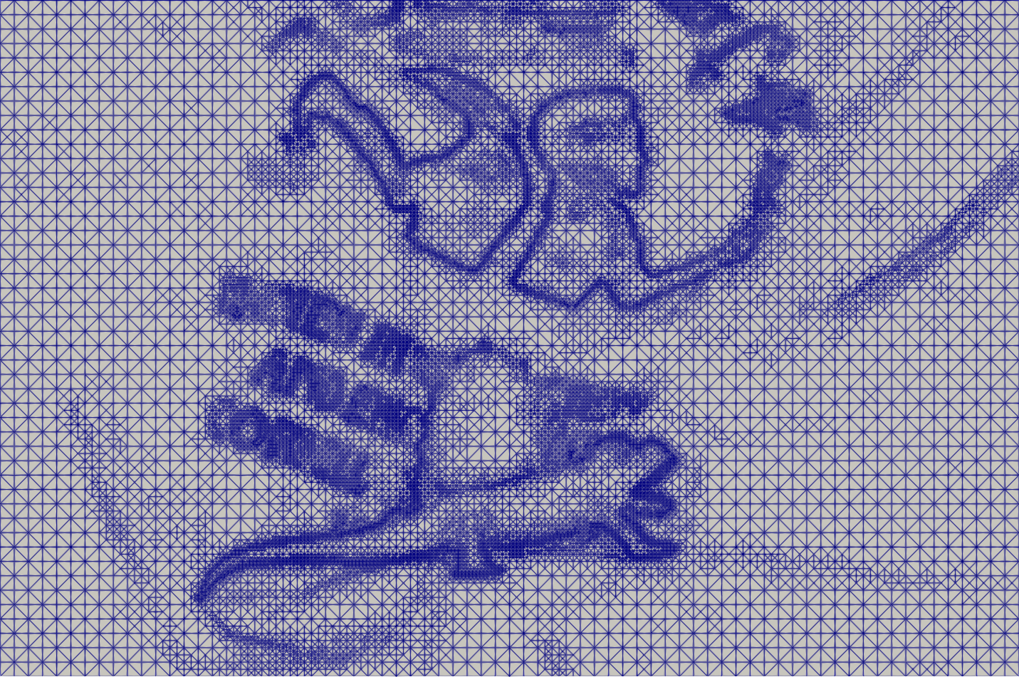
Figure 6: Exemplary adapted mesh for LABEL:alg:optflow_adapt on the Dimetrodon Middlebury optical flow benchmark.

We note that for $S=I$ very similar qualitative and quantitative results are obtained, see section 3.1. A reason for this might be that we choose $\beta=0.00$, which is rather small and hence the choice of $S$ does not play a crucial role for numerically computing a solution. Indeed, as the associated term $\mathchoice{\tfrac{\beta}{2}}{\frac{\beta}{2}}{\frac{\beta}{2}}{\frac{\beta}{2}}\|S\mathbf{u}\|_{V_{S}}^{2}$ is only added for theoretical reasons, one typically wants to choose $\beta$ very small [21].

& $0.43$ $0.40$ $0.14$ $0.13$ $79.52$ LABEL:alg:optflow_adapt (with l2-pixel) $0.43$ $0.39$ $0.14$ $0.12$ $60.89$

Grove2 [21, Algorithm 3] without warping $2.93$ $0.46$ $1.10$ $0.14$ $195.36$ [21, Algorithm 3] with warping $1.13$ $1.30$ $0.42$ $0.54$ $1{,}689.12$ LABEL:alg:optflow_adapt (with l2lagrange) $0.40$ $0.57$ $0.11$ $0.16$ $134.80$ LABEL:alg:optflow_adapt (with l2-pixel) $0.39$ $0.56$ $0.11$ $0.16$ $109.99$

Grove3 [21, Algorithm 3] without warping $3.69$ $2.33$ $1.01$ $0.32$ $211.27$ [21, Algorithm 3] with warping $1.93$ $2.10$ $0.27$ $0.29$ $1{,}579.88$ LABEL:alg:optflow_adapt (with l2lagrange) $1.14$ $1.51$ $0.17$ $0.29$ $152.71$ LABEL:alg:optflow_adapt (with l2-pixel) $1.12$ $1.49$ $0.16$ $0.29$ $151.63$

Hydrangea [21, Algorithm 3] without warping $3.33$ $1.22$ $0.91$ $0.23$ $151.16$ [21, Algorithm 3] with warping $0.22$ $0.52$ $0.04$ $0.10$ $1{,}303.31$ LABEL:alg:optflow_adapt (with l2lagrange) $0.60$ $0.50$ $0.08$ $0.12$ $86.75$ LABEL:alg:optflow_adapt (with l2-pixel) $0.57$ $0.47$ $0.08$ $0.11$ $72.85$

RubberWhale [21, Algorithm 3] without warping $0.67$ $0.58$ $0.36$ $0.25$ $187.59$ [21, Algorithm 3] with warping $0.26$ $0.52$ $0.14$ $0.26$ $624.25$ LABEL:alg:optflow_adapt (with l2lagrange) $0.39$ $0.59$ $0.21$ $0.33$ $65.65$ LABEL:alg:optflow_adapt (with l2-pixel) $0.39$ $0.60$ $0.21$ $0.33$ $57.27$

Urban2 [21, Algorithm 3] without warping $8.16$ $8.12$ $0.99$ $0.40$ $212.86$ [21, Algorithm 3] with warping $7.62$ $8.15$ $0.64$ $0.39$ $637.57$ LABEL:alg:optflow_adapt (with l2lagrange) $4.52$ $5.26$ $0.28$ $0.32$ $83.84$ LABEL:alg:optflow_adapt (with l2-pixel) $5.03$ $5.76$ $0.32$ $0.34$ $69.16$

Urban3 [21, Algorithm 3] without warping $7.04$ $4.45$ $1.13$ $0.24$ $242.47$ [21, Algorithm 3] with warping $5.57$ $4.45$ $0.50$ $0.40$ $1{,}062.80$ LABEL:alg:optflow_adapt (with l2lagrange) $1.76$ $2.34$ $0.25$ $0.50$ $127.76$ LABEL:alg:optflow_adapt (with l2-pixel) $1.82$ $2.35$ $0.26$ $0.50$ $100.39$

Venus [21, Algorithm 3] without warping $3.55$ $1.75$ $1.00$ $0.24$ $121.23$ [21, Algorithm 3] with warping $1.25$ $1.52$ $0.23$ $0.35$ $887.40$ LABEL:alg:optflow_adapt (with l2lagrange) $0.73$ $1.13$ $0.15$ $0.34$ $79.46$ LABEL:alg:optflow_adapt (with l2-pixel) $0.75$ $1.14$ $0.15$ $0.34$ $80.27$

Table 4: Results for $S=I$: Endpoint errors (EE) and angular errors (AE) as in [3], each given by mean and standard deviation, and computational time in seconds.

Acknowledgment

This work was partly supported by the Ministerium für Wissenschaft, Forschung und Kunst of Baden-Württemberg (Az: 7533.-30-10/56/1) through the RISC-project “Automatische Erkennung von bewegten Objekten in hochauflösenden Bildsequenzen mittels neuer Gebietszerlegungsverfahren”, by the Deutsche Forschungsgemeinschaft (DFG, German Research Foundation) under Germany’s Excellence Strategy – EXC 2075 – 390740016, and by the Crafoord Foundation through the project “Locally Adaptive Methods for Free Discontinuity Problems”.

References

- [1] M. Ainsworth and J. T. Oden. A Posteriori Error Estimation in Finite Element Analysis. Wiley-Interscience, New York, 2000.
- [2] M. Alkämper and A. Langer. Using DUNE-ACFem for Non-smooth Minimization of Bounded Variation Functions. Archive of Numerical Software, 5(1):3–19, 2017.
- [3] S. Baker, D. Scharstein, J. Lewis, S. Roth, M. J. Black, and R. Szeliski. A database and evaluation methodology for optical flow. International Journal of Computer Vision, 92(1):1–31, 2011.
- [4] E. Bänsch and K. Mikula. A coarsening finite element strategy in image selective smoothing. Computing and Visualization in Science, 1(1):53–61, 1997.
- [5] S. Bartels. Total Variation Minimization with Finite Elements: Convergence and Iterative Solution. SIAM Journal on Numerical Analysis, 50(3):1162–1180, 2012.
- [6] S. Bartels. Error Control and Adaptivity for a Variational Model Problem Defined on Functions of Bounded Variation. Mathematics of Computation, 84(293):1217–1240, 2015.
- [7] S. Bartels. Numerical Methods for Nonlinear Partial Differential Equations, volume 14. Springer, 2015.
- [8] S. Bartels and M. Milicevic. Primal-dual gap estimators for a posteriori error analysis of nonsmooth minimization problems. ESAIM: Mathematical Modelling and Numerical Analysis, 54(5):1635–1660, 2020.
- [9] C. Bazan and P. Blomgren. Adaptive finite element method for image processing. In Proceedings of COMSOL Multiphysics Conference, pages 377–381, 2005.
- [10] Z. Belhachmi and F. Hecht. Control of the effects of regularization on variational optic flow computations. Journal of Mathematical Imaging and Vision, 40(1):1–19, 2011.
- [11] Z. Belhachmi and F. Hecht. An adaptive approach for the segmentation and the TV-filtering in the optic flow estimation. Journal of Mathematical Imaging and Vision, 54(3):358–377, 2016.
- [12] J. Bezanson, A. Edelman, S. Karpinski, and V. B. Shah. Julia: A fresh approach to numerical computing. SIAM review, 59(1):65–98, 2017.
- [13] K. Bredies and D. Lorenz. Mathematical Image Processing. Applied and Numerical Harmonic Analysis. Birkhäuser, 1 edition, 2018.
- [14] F. Brezzi, J. Douglas, and L. D. Marini. Two families of mixed finite elements for second order elliptic problems. Numerische Mathematik, 47:217–235, 1985.
- [15] F. Catté, P.-L. Lions, J.-M. Morel, and T. Coll. Image selective smoothing and edge detection by nonlinear diffusion. SIAM Journal on Numerical Analysis, 29(1):182–193, 1992.
- [16] A. Chambolle and T. Pock. Approximating the total variation with finite differences or finite elements. In Handbook of Numerical Analysis, volume 22, pages 383–417. Elsevier, 2021.
- [17] H. Dirks. Variational methods for joint motion estimation and image reconstruction. PhD thesis, Universitäts-und Landesbibliothek Münster, 2015.
- [18] I. Ekeland and R. Témam. Convex Analysis and Variational Problems, volume 28 of Classics in Applied Mathematics. Society for Industrial and Applied Mathematics (SIAM), Philadelphia, PA, english edition, 1999. Translated from the French.
- [19] A. Ern and J.-L. Guermond. Finite element quasi-interpolation and best approximation. ESAIM: Mathematical Modelling and Numerical Analysis, 51(4):1367–1385, 2017.
- [20] S. Hilb. https://gitlab.mathematik.uni-stuttgart.de/stephan.hilb/semismoothnewton.jl.
- [21] S. Hilb, A. Langer, and M. Alkämper. A primal-dual finite element method for scalar and vectorial total variation minimization. Journal of Scientific Computing, 96(1):24, 2023.
- [22] M. Hintermüller and A. Langer. Subspace Correction Methods for a Class of Nonsmooth and Nonadditive Convex Variational Problems with Mixed Data-fidelity in Image Processing. SIAM Journal on Imaging Sciences, 6(4):2134–2173, 2013.
- [23] M. Hintermüller and M. Rincon-Camacho. An Adaptive Finite Element Method in -TV-based Image Denoising. Inverse Problems and Imaging, 8(3):685–711, 2014.
- [24] A. Langer. Automated parameter selection in the --TV model for removing Gaussian plus impulse noise. Inverse Problems, 33(7):074002, 2017.
- [25] A. Langer. Locally adaptive total variation for removing mixed Gaussian–impulse noise. International Journal of Computer Mathematics, 96(2):298–316, 2019.
- [26] J. Necas. Direct methods in the theory of elliptic equations. Springer Science & Business Media, 2011.
- [27] R. H. Nochetto, K. G. Siebert, and A. Veeser. Theory of adaptive finite element methods: An introduction. In Multiscale, nonlinear and adaptive approximation, pages 409–542. Berlin: Springer, 2009.
- [28] T. Preußer and M. Rumpf. An adaptive finite element method for large scale image processing. Journal of Visual Communication and Image Representation, 11(2):183–195, 2000.
- [29] C. E. Shannon. A mathematical theory of communication. The Bell System Technical Journal, 27(4):623–656, 1948.
- [30] R. Verfürth. A posteriori error estimation techniques for finite element methods. OUP Oxford, 2013.
- [31] Z. Wang, A. C. Bovik, H. R. Sheikh, and E. P. Simoncelli. Image quality assessment: from error visibility to structural similarity. IEEE Transactions on Image Processing, 13(4):600–612, 2004.