Suppressing the sample variance of DESI-like galaxy clustering with fast simulations

Abstract

Ongoing and upcoming galaxy redshift surveys, such as the Dark Energy Spectroscopic Instrument (DESI) survey, will observe vast regions of sky and a wide range of redshifts. In order to model the observations and address various systematic uncertainties, $N$-body simulations are routinely adopted, however, the number of large simulations with sufficiently high mass resolution is usually limited by available computing time. Therefore, achieving a simulation volume with the effective statistical errors significantly smaller than those of the observations becomes prohibitively expensive. In this study, we apply the Convergence Acceleration by Regression and Pooling (CARPool) method to mitigate the sample variance of the DESI-like galaxy clustering in the AbacusSummit simulations, with the assistance of the quasi-$N$-body simulations FastPM. Based on the halo occupation distribution (HOD) models, we construct different FastPM galaxy catalogs, including the luminous red galaxies (LRGs), emission line galaxies (ELGs), and quasars, with their number densities and two-point clustering statistics well matched to those of AbacusSummit. We also employ the same initial conditions between AbacusSummit and FastPM to achieve high cross-correlation, as it is useful in effectively suppressing the variance. Our method of reducing noise in clustering is equivalent to performing a simulation with volume larger by a factor of $5$ and $4$ for LRGs and ELGs, respectively. We also mitigate the standard deviation of the LRG bispectrum with the triangular configurations $k_{2}=2k_{1}=0.2\,h\,\mathrm{Mpc}^{-1}$ by a factor of 1.6. With smaller sample variance on galaxy clustering, we are able to constrain the BAO scale parameters to higher precision. The CARPool method will be beneficial to better constrain the theoretical systematics of BAO, redshift space distortions (RSD) and primordial non-Gaussianity.

1 Introduction

The Dark Energy Spectroscopic Instrument (DESI) is an ongoing Stage IV spectroscopic redshift survey [1, 2, 3, 4]. DESI will cover a large sky area $\sim 14000$ deg² and a wide redshift range $0<z<3.5$, targeting different tracers of dark matter distribution, i.e. the bright galaxy samples (BGS) at $0<z<0.4$ [5], luminous red galaxies (LRGs) at $0.4<z<1.1$ [6], emission line galaxies (ELGs) at $1.1<z<1.6$ [7], quasars (QSOs) at $0.9<z<2.1$ [8], and Lyman alpha (Ly-$\alpha$) forest at $2.1<z<3.5$. At the end of survey, DESI is going to collect over $40$ million extra-galactic spectra of galaxies and quasars, one order of magnitude larger than the spectra from the previous galaxy redshift surveys, e.g. the 2-degree Field Galaxy Redshift Survey [9], the WiggleZ Dark Energy Survey [10], the 6-degree Field Galaxy Survey [11], and the Sloan Digital Sky Survey [12, 13, 14, 15, 16, 17, 18] combined together. Taking BAO as a standard ruler, DESI is able to measure the cosmological distances at sub-per cent level [4], which dramatically tightens the constraints on the expansion rate of the Universe and the dark energy models. Meanwhile, DESI measures the redshift space distortions (RSD), which is originated from the peculiar motions of galaxies. RSD adds anisotropy on the measured galaxy clustering signal [19, 20]. Measuring RSD can directly probe the structure growth rate and the amount of matter in the Universe, hence, it is essential to constrain gravity models [21, 22, 18]. In addition, we can probe primordial non-Gaussianity (NG) from high-order galaxy clustering statistics, such as bispectrum [23, 24]. For the case of local NG, it would induce a scale-dependent galaxy bias proportional to $k^{-2}$ on galaxy power spectrum [25]. Several studies have been conducted recently to constrain the local NG parameter $f_{\mathrm{nl}}$, e.g. [26, 27, 28, 29, 30].

Besides DESI, other forthcoming Stage IV galaxy surveys including the Euclid space telescope [31], the Prime Focus Spectrograph [32], the China Space Station Telescope [33], and the Nancy Grace Roman Space Telescope [34], will dramatically increase the survey volumes and sample size. In order to interpret the observation and calibrate different systematic errors for cosmological analysis, we widely refer to $N$-body simulations. In DESI, the flagship $N$-body simulation is AbacusSummit [35]. Due to its large volume and high mass resolution, the number of AbacusSummit simulations is limited, e.g. 25 base boxes for the primary cosmology. But for other cosmologies the number of simulations is less, and there is only one simulation for most of cosmologies. Comparing the simulation box size $8\,h^{-3}\mathrm{Gpc}^{3}$ with the DESI effective survey volume $\sim 20\,h^{-3}\mathrm{Gpc}^{3}$ [4], the sample variance of simulations will be larger than that of DESI data.

There have been several methods proposed to mitigate the sample variance of simulations. [36] proposed the fixed and paired method, which utilizes a paired initial conditions (ICs) with the fixed amplitude and inverse phases. With a small number of the paired simulations, it can significantly suppress the sample variance of dark matter, halo and galaxy two-point clustering statistics on large scales without introducing bias [e.g. 37, 38, 39]. It has been applied and studied in various simulations, e.g. [40, 41, 42]. Another method recently proposed is adopting the principle of control variates, including the simulation based one and the theory based one. The former utilizes fast simulations or surrogates to construct the control variates [43, 44, 45], while the latter theoretically predicts the control variates [46, 47, 48, 49]. The analytic control variates only require ICs without running a number of surrogates as needed for the simulation based one, hence, it can save quite amount of computational time. However, currently it is only available to model galaxy two-point clustering but not for higher order statistics, e.g. bispectrum. In addition, it is not trivial to include some observational systematics, such as fiber collision, in the theoretical template, while it is straightforward for simulations. In this study, we focus on the simulation based method, and study the performance of the sample variance suppression on galaxy clustering.

Galaxies form in dark matter halos and are tracers of dark matter distribution. In cosmological simulations with dark matter only, we directly simulate the spatial distribution and motion of dark matter particles. Then we define some gravitational bounded regions with particles concentrated as dark matter halos. After that, we generate the galaxy distribution by painting galaxies into halos based on some galaxy-halo connection schemes varying from more physical to more empirical ones (see a recent review [50]). The halo occupation distribution (HOD) is a phenomenological model [51, 52, 53], which models the distribution of central and satellite galaxies separately. In this study, we apply the HOD models to generate FastPM galaxy catalogs, whose number density and galaxy clustering are matched to those of AbacusSummit.

Our paper is constructed as follows. In section 2, we summarize the details of AbacusSummit and FastPM simulations. In section 3, we introduce the HOD models, the HOD fitting process, and the CARPool method. In section 4, we describe the galaxy clustering statistics that we study. In section 5, we show the comparison of the FastPM and AbacusSummit galaxy clustering, the suppression on the sample variance of the AbacusSummit galaxy clustering and the increased BAO constraints from CARPool. In section 6, we make conclusions and discussions.

2 Simulations

2.1 AbacusSummit

AbacusSummit is a large suite of high-accuracy $N$-body simulations prepared for the DESI survey. The simulations were generated at the Summit supercomputer of the Oak Ridge National Laboratory using the Abacus code [54]. AbacusSummit covers different cosmologies. In our study, we focus on the simulations with the primary cosmology, denoted as c000, which is the $\Lambda$CDM model with the cosmological parameters constrained from the Planck 2018 result (TT,TE,EE+lowE+lensing) [55]. AbacusSummit also covers different box sizes and mass resolutions of dark matter particles. There are 25 base boxes with the cosmology c000 but different initial conditions (ICs), denoted as ph0[00-24]. Each realization has the box size $2\,h^{-1}\mathrm{Gpc}$ per side and contains $6912^{3}$ particles with mass equal to $\sim 2.1\times 10^{9}\,h^{-1}\mathrm{M}_{\odot}$. AbacusSummit utilizes compaso to identify dark matter halos and adopts a cleaning method to remove spuriously identified halos [56]. Based on the cleaned halo catalogs at different redshifts, different types of galaxy catalogs have been generated using HOD. We describe the HOD models in section 3.1. The best-fit HOD parameters are obtained from fitting the AbacusSummit galaxy clustering to the observed one from the DESI One-Percent Survey [58]. Therefore, the obtained galaxy catalogs with the best-fit HOD have similar galaxy clustering as the true one that DESI will observe, ignoring any effects from survey footprint, observational systematics, and fiber assignment. We call these galaxy catalogs as DESI-like samples. Table 1 displays the basic information of the DESI-like catalogs for different tracers.

	redshift	$n$ [$10^{-4}\,h^{3}\mathrm{Mpc}^{-3}$]	bias	$f$
LRGs	0.8	10	2.0	0.838
ELGs	1.1	30	1.2	0.888
QSOs	1.4	1.3	2.1	0.920

Table 1: The redshift, galaxy number density, galaxy bias and growth rate of the cubic DESI-like galaxy catalogs from AbacusSummit.

2.2 FastPM

FastPM is a type of quasi-$N$-body simulations [59]. It implements the Particle-Mesh (PM) scheme with modified kick and drift factors to ensure that the linear growth of displacement agrees with the Zel’dovich approximation at large scales. With a lower mass resolution compared to the $N$-body simulation (e.g. AbacusSummit) and a few time steps ($\sim 40$), FastPM is able to recover the matter power spectrum up-to $k\sim 1\,h\,\mathrm{Mpc}^{-1}$ within $2$ per cent level accuracy [60]. FastPM uses Friends-of-Friends (FoF) algorithm to find dark matter halos. In addition, several methods have been proposed to further improve the FastPM matter and halo clustering at small scales [61, 62]. Meanwhile, [63] implements the contribution of neutrinos in FastPM. [64] populates galaxies in FastPM halos based on HOD, and makes the galaxy clustering well matched to that of AbacusSummit.

In our study, we utilize the FastPM simulations generated in [45], which contains $25$ realizations with the cosmology c000 and the same ICs as the AbacusSummit base boxes. In addition, we have generated $313$ boxes with random (nonfixed-amplitude) ICs. The simulation box has size of $2\,h^{-1}\mathrm{Gpc}$ per side and $5184^{3}$ particles with mass resolution $\sim 5\times 10^{9}\,h^{-1}\mathrm{M}_{\odot}$. The force resolution is set by the parameter $B=N_{m}/N_{g}=2$, where $N_{m}$ and $N_{g}$ are the number of the mesh size and galaxies per side of box, respectively. Simulations start from the initial redshift $19$ to $0.1$ with $40$ time steps linearly separated in scale $a=\frac{1}{1+z}$. One simulation takes about $50$ minutes using 1152 KNL nodes each with 68 CPU cores and 98 GB memory based on the Cori supercomputer at NERSC. Although the computational cost is much cheaper than that of $N$-body simulation, it is still costly to run a number of FastPM with such configuration. To populate galaxies in FastPM halos, we select halos with mass larger than $5\times 10^{10}\,h^{-1}\mathrm{M}_{\odot}$. The particle mass resolution in our simulation is close to the low resolution one of [64], which uses a halo mass cut similar to ours, and gives reliable HOD fitting. We have also tested using a higher halo mass cut, and found that it does not affect our final result.

3 Methodology

3.1 HOD models

We describe the HOD models used to populate different types of galaxies in the AbacusSummit and FastPM catalogs. We also notify some modifications on the FastPM HOD models.

3.1.1 LRGs

At $0.4<z<1.1$, DESI mainly observe LRGs, which are relatively easy to select with their characteristic 4000 $\mathring{A}$ break in the spectra. They are assumed to inhabit massive halos and have high galaxy biases. We adopt the vanilla HOD model based on [53] for AbacusSummit LRGs. In this model, the distribution of central galaxies follows a Bernoulli distribution with the mean occupation number given by

$$\langle N_{\text{cent}}^{\text{LRG}}\rangle=\frac{1}{2}\bigg{[}1+\text{erf}\Big{(}\frac{\log M_{\text{h}}-\log M_{\text{cut}}}{\sqrt{2}\sigma_{\log M_{\text{h}}}}\Big{)}\bigg{]},$$ (3.1)

where $M_{\text{h}}$ is the halo mass, $M_{\text{cut}}$ is the halo mass limit at which half of the halos host one central galaxy on average, $\log$ denotes the 10 based logarithm, and erf is the error function, i.e.

$$\text{erf}(x)=\frac{2}{\sqrt{\pi}}\int_{0}^{x}e^{-t^{2}}dt.$$ (3.2)

The distribution of satellite galaxies follows a Poisson distribution. The mean number distribution follows a power low, i.e.

$$\langle N_{\text{sat}}^{\text{LRG}}\rangle=\bigg{(}\frac{M_{\text{h}}-\kappa M_{\text{cut}}}{M_{1}}\bigg{)}^{\alpha},$$ (3.3)

where $\kappa M_{\text{cut}}$ denotes the minimum mass that halos can host satellite galaxies, $M_{1}$ is the halo mass at which halos host on average one satellite galaxy, and $\alpha$ is the slope of the power-law function. For the spatial distribution of satellites, it follows the Navarro-Frenk-White profile [65]. We assign velocities to satellites based on a Gaussian distribution with the mean halo velocity and the velocity distribution of dark matter particles inside a halo.

To make the FastPM galaxy clustering match with that of AbacusSummit better in redshift space, we add an additional parameter $v_{\text{disp}}$ on top of the default model [64]. It modifies velocities along the line of sight (LoS) for the FastPM satellites, i.e.

$$v^{\text{sat, modified}}_{\parallel}=(v^{\text{sat, default}}_{\parallel}-v^{\text{halo}}_{\parallel})\times v_{\text{disp}}+v^{\text{halo}}_{\parallel},$$ (3.4)

where the subscript $\parallel$ denotes parallel to the LoS. In this study, we include $v_{\text{disp}}$ in all the FastPM HOD models.

3.1.2 ELGs

At $0.8<z<1.6$, DESI observes the primary galaxy samples with strong [O II] doublet $\lambda\lambda$ 3726,29 $\mathring{A}$ emission lines, denoted as ELGs, which are sub-samples of the star-forming galaxies. Star forming process depends on halo mass and environment. For central ELGs living in more massive halos, they are more likely to quench, hence, the canonical step function cannot fully describe the distribution. The high mass quenching model [66, 67, 68] works quite well for central ELGs, and it models the mean number distribution as

$$\langle N_{\text{cen}}^{\text{ELG}}\rangle=2A\phi(M)\Phi(\gamma M)+\frac{1}{2Q}\bigg{[}1+\text{erf}\bigg{(}\frac{\text{log}M_{h}-\text{log}M_{\text{cut}}}{0.01}\bigg{)}\bigg{]}.$$ (3.5)

where

$$\phi(x) =\mathcal{N}(\log M_{\text{cut}},\sigma_{\text{log}M_{\text{h}}}),$$ (3.6)

$$\Phi(x) =\int_{-\infty}^{x}\phi(x^{\prime})dx^{\prime}=\frac{1}{2}\bigg{[}1+\text{erf}\bigg{(}\frac{x}{\sqrt{2}}\bigg{)}\bigg{]},$$ (3.7)

$$A =\frac{p_{\max}-1/Q}{\text{max}(2\phi(x)\Phi(\gamma x))}.$$ (3.8)

$\mathcal{N}$ denotes the Gaussian distribution, $Q$ models the galaxy quenching efficiency at massive halos, $p_{\text{max}}$ sets the saturation level of the occupation probability, and $\gamma$ is a skewness parameter. We refer the readers to [68] for more detailed study on these parameters. For the FastPM centrals, we only adopt the first part of eq. 3.5 to populate. For the AbacusSummit ELG satellites, the mean number distribution follows the same relation as the LRGs’ (eq. 3.3). Recent studies have found that the galactic conformity has strong effect on the population of satellites. Satellites are more likely to inhabit halos with central galaxies are ELGs [69, 70, 71]. Such galactic conformity can boost the one-halo term clustering at very small scales. We leave the study of galactic conformity in future work.

3.1.3 QSOs

QSOs are luminous point-like sources, generated by the accretion of matter onto super-massive black holes in centers of galaxies. DESI observes QSOs as direct tracers at $0.9<z<2.1$, and takes them as backlights for the Ly $\alpha$ forest at $2.1<z<3.6$. Here, we only consider the QSOs as direct tracers. For the central distribution of AbacusSummit QSOs, it is the same as the LRGs’ but with the downsampling parameter $p_{\text{max}}$ that models the duty cycle of QSOs [68, 72], i.e.

$$\langle N_{\text{cent}}^{\text{QSO}}\rangle=\frac{1}{2}p_{\text{max}}\bigg{[}1+\text{erf}\Big{(}\frac{\log M_{\text{h}}-\log M_{\text{cut}}}{\sqrt{2}\sigma_{\log M_{\text{h}}}}\Big{)}\bigg{]},$$ (3.9)

For the distribution of satellites, it follows eq. 3.3 as well.

3.2 HOD fitting process

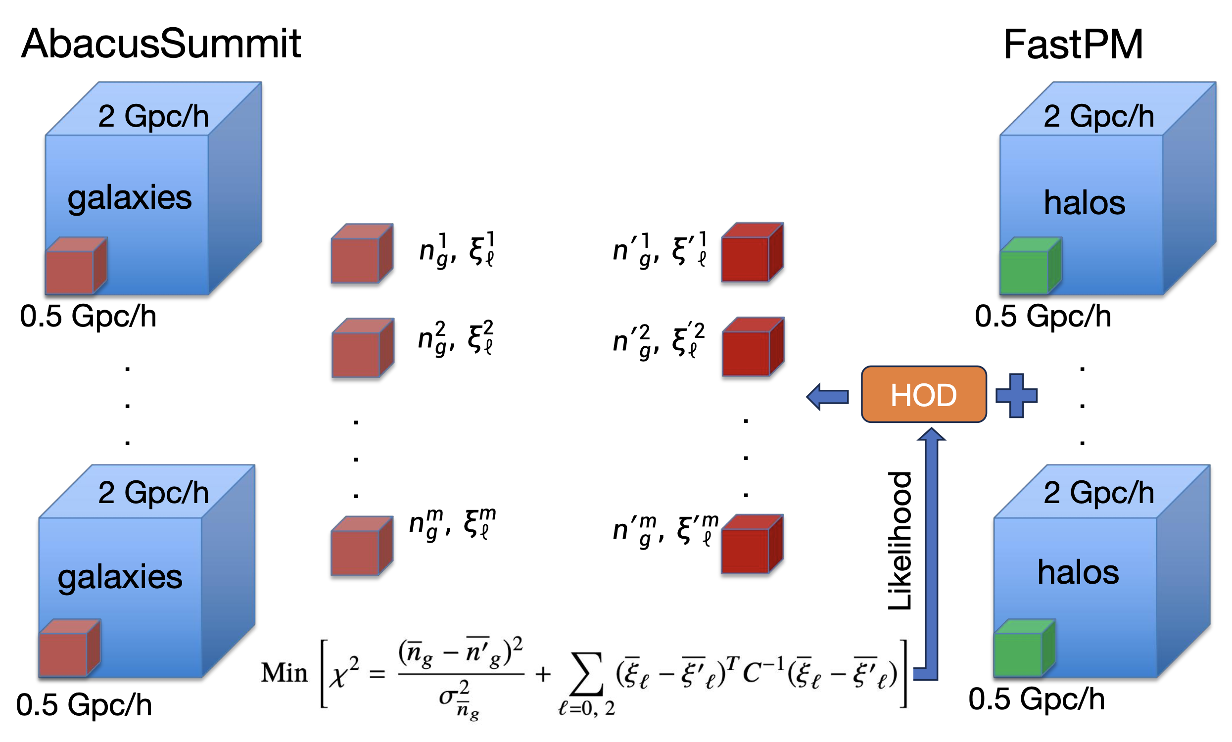
Figure 1: A cartoon diagram showing the flowchart of the HOD fitting process. Given an AbacusSummit galaxy catalog with the original box size $(2\,h^{-1}\mathrm{Gpc})^{3}$, we cut out a $500\,h^{-1}\mathrm{Mpc}$ sub-box. For the sub-box, we calculate the galaxy number density and two-point clustering statistics. From a paired FastPM simulation with the AbacusSummit IC, we cut out the same sub-box, and populate galaxies in the halos given a HOD model. To find the optimal HOD parameters, we compare the galaxy number density and two-point clustering, and minimize the difference between the two galaxy catalogs. In order to reduce the sample variance, we compare the mean galaxy number density and clustering over a number of the paired sub-boxes. We use the nested sampling to find the best-fit HOD parameters.

To find the optimal HOD parameters, we follow the routine described in [64] with some modifications. Basically, we match the FastPM galaxy number density $n_{\text{g}}$ and galaxy two-point clustering $\xi_{\ell}$ (or $P_{\ell}$) to those of AbacusSummit. We find the best FastPM HOD parameters via minimizing

$$\chi^{2}=(D-M)^{T}\Sigma^{-1}(D-M),$$ (3.10)

where $D$ and $M$ denotes data (observation) and model prediction, respectively, and $\Sigma$ is the covariance matrix of $D$.

Since we have the paired FastPM with the AbacusSummit ICs, some of the sample variance can be cancelled out when we compare the galaxy statistics from the two simulations, especially at larger scales. We consider the data as the difference of the galaxy number density and clustering from FastPM and AbacusSummit, i.e. $D\rightarrow D_{\text{F}}-D_{\text{A}}$ with the subscripts F and A denoting FastPM and AbacusSummit, respectively. Ideally, we expect that $D_{\text{F}}$ can match closely to $D_{\text{A}}$, given some optimal HOD parameters, hence, the model expectation of $D_{\text{F}}-D_{\text{A}}$ is close to 0, i.e. $M\rightarrow 0$. We can transform eq. 3.10 to

$$\chi^{2}\simeq(D_{\text{F}}-D_{\text{A}})^{T}\Sigma_{\text{diff}}^{-1}(D_{\text{F}}-D_{\text{A}}),$$ (3.11)

where $\Sigma_{\text{diff}}$ is the covariance matrix of $D_{\text{F}}-D_{\text{A}}$. However, we do not know $\Sigma_{\text{diff}}$ without having FastPM galaxy catalogs. To resolve that, our fitting process consists of two steps.

For the first-step fitting, we aim to get initial guess on the FastPM HOD, so that it more or less reproduces the AbacusSummit clustering. This will allow us to obtain a first estimate of the difference covariance matrix $\Sigma_{\text{diff}}$. We then use such difference covariance matrix to run the second step of fitting and obtain the final HOD parameter for the FastPM simulations.

In the first step, we consider the AbacusSummit galaxy statistics as the model, to which we fit the FastPM statistics. Instead of using the original $2\,h^{-1}\mathrm{Gpc}$ boxes, we choose sub-boxes to perform HOD fitting for two reasons. Firstly, it is computationally more efficient to populate galaxies and calculate the clustering given a set of sub-boxes thanks to the smaller volume. It is especially necessary for the case when we need to perform such process multiple times during the HOD fitting with some sampling method. Secondly, we can construct a covariance matrix $\Sigma$ from the sub-boxes. In our case, we cut each AbacusSummit box into 64 sub-boxes, each of which has side length $500\,h^{-1}\mathrm{Mpc}$. We compute the galaxy number density and clustering for each sub-box, and get the covariance matrix from 1600 ($25\times 64$) AbacusSummit sub-boxes. Given that we only want to estimate the best-fit in this step, we simply use the diagonal terms of the covariance matrix, i.e.

$$\Sigma=\text{Diag}\bigg{[}\sigma^{2}_{\xi_{1}(s_{1})}\;\sigma^{2}_{\xi_{1}(s_{2})}\;\cdots\;\sigma^{2}_{\xi_{1}(s_{N})}\;\sigma^{2}_{\xi_{2}(s_{1})}\,\sigma^{2}_{\xi_{2}(s_{2})}\;\cdots\;\sigma^{2}_{\xi_{2}(s_{N})}\;\sigma^{2}_{n_{\text{g}}}\bigg{]},$$ (3.12)

where we consider the correlation function monopole and quadrupole, as well as the galaxy number density; $s_{1}$, $s_{2}$, $\cdots$, $s_{N}$ denote the radial coordinates of the multipoles. We set $s_{1}=2\,h^{-1}\mathrm{Mpc}$, $s_{N}=46\,h^{-1}\mathrm{Mpc}$, and the step size equal to $4\,h^{-1}\mathrm{Mpc}$. Our results are not very sensitive to these choices, and the large scale limit $s_{N}$ chosen is to keep the model computation efficient.

For FastPM, we cut out the sub-boxes with the same way as AbacusSummit. Given some HOD model, we can populate the FastPM halos with galaxies in the sub-boxes. To reduce the sample variance, we calculate the mean galaxy number density and two-point clustering from a number of sub-boxes, and compare them with those from the paired AbacusSummit sub-boxes. Minimizing the difference between the two based on eq. 3.10, we can find the best-fit HOD parameters. We use the fitting pipeline hodor, which implements halotools [73], and utilizes PyMultiNest [74, 75, 76, 77] as a nested sampling Monte Carlo library. We show the demonstration of the HOD fitting process in figure 1.

For the second-step fitting, we first obtain the FastPM galaxy catalogs based on the best-fit HOD parameters from the first-step fitting. Then we cut 25 FastPM ($2\,h^{-1}\mathrm{Gpc}$) boxes into 1600 ($500\,h^{-1}\mathrm{Mpc}$) sub-boxes. We calculate the covariance matrix of the difference of the two-point galaxy clustering ($D_{\text{A}}-D_{\text{F}}$) between AbacusSummit and FastPM, denoted as $\mathbb{C}$. We concatenate $\mathbb{C}$ with the variance of the galaxy number density to get

$$\Sigma_{\text{diff}}=\begin{pmatrix}\mathbb{C}&0\\ 0&\sigma^{2}_{n_{\text{g}}}\\ \end{pmatrix},$$ (3.13)

We plug $\Sigma_{\text{diff}}$ into eq. 3.10 and obtain the final HOD fitting parameters. Note that the two-point clustering can be the correlation function, power spectrum, or the two combined. We have tested that using the power spectrum monopole and quadrupole with the fitting range $0.02\,h\,\mathrm{Mpc}^{-1}\leq k\leq 0.5\,h\,\mathrm{Mpc}^{-1}$ and the step size $0.02\,h\,\mathrm{Mpc}^{-1}$ gives reliable HOD fitting parameters. We show the best-fit FastPM HOD parameters for the FastPM LRGs, ELGs, and QSOs in table 3.

3.3 CARPool method

Given a limited number of $N$-body simulations, the measured clustering signal has large sample variance. The CARPool method, short for Convergence Acceleration by Regression and Pooling, firstly proposed by [43], is a straightforward way to mitigate the sample variance. It utilizes the principle of control variates. Starting from the scalar case, supposing $y$ is an observable from an $N$-body simulation, we can construct a new observable $x$ as

$$x=y-\beta(c-\mu_{c}),$$ (3.14)

where $c$ is the same observable from a paired fast simulation or surrogate using the same IC as the $N$-body simulation, $\beta$ is a coefficient, and $\mu_{c}$ is the expected mean of $c$. Note that $\mu_{c}$ can be modeled by theory or estimated from a number of simulations with random ICs. Since the ICs of $c$ and $\mu_{c}$ are different, there will be no cross-correlation between $c$ and $\mu_{c}$. Based on eq. 3.14, the expectation of $x$ is unbiased from that of $y$, i.e. $\langle x\rangle=\langle y\rangle$, since $\langle c\rangle=\mu_{c}$. In addition, the sample variance of $x$ is

$$\sigma^{2}_{x}=\sigma^{2}_{y}-2\beta\text{cov}(y,c)+\beta^{2}\sigma^{2}_{c}+\beta^{2}\sigma^{2}_{\mu_{c}},$$ (3.15)

where $\text{cov}(y,c)$ is the covariance between $y$ and $c$. We aim to make $\sigma^{2}_{x}<\sigma^{2}_{y}$ from CARPool. By varying the coefficient $\beta$ to have $\frac{\partial\sigma^{2}_{x}}{\partial\beta}=0$, we can minimize $\sigma^{2}_{x}$. So we get

$$\beta=\frac{\text{cov}(y,c)}{\sigma^{2}_{c}+\sigma^{2}_{\mu_{c}}}\simeq\frac{\text{cov}(y,c)}{\sigma_{c}^{2}}.$$ (3.16)

The second equation holds if $\mu_{c}$ is from theoretical prediction (i.e. $\sigma_{\mu_{c}}=0$) or from a large number of surrogates (i.e. $\sigma_{\mu_{c}}\ll\sigma_{c}$). Substituting eq. 3.16 into eq. 3.15, we have

$$\frac{\sigma_{x}^{2}}{\sigma_{y}^{2}}=1+\rho^{2}_{y,c}\bigg{(}\frac{\sigma^{2}_{\mu_{c}}}{\sigma^{2}_{c}}-1\bigg{)},$$ (3.17)

where $\rho_{y,c}=\text{cov}(y,c)/(\sigma_{y}\sigma_{c})$ is the Pearson correlation coefficient between $y$ and $c$. The larger cross-correlation between $y$ and $c$ (as $\rho_{y,c}\rightarrow 1$) and smaller $\sigma^{2}_{\mu_{c}}$, the smaller the sample variance of $x$ will be. In addition, we can derive the ratio of the variance of the mean $x$ and $y$ over $N$ realizations, i.e.

$$\frac{\sigma_{\overline{x}}^{2}}{\sigma_{\overline{y}}^{2}}=1+\rho^{2}_{y,c}\bigg{(}N\frac{\sigma^{2}_{\mu_{c}}}{\sigma^{2}_{c}}-1\bigg{)},$$ (3.18)

where we assume that the same $\mu_{c}$ is used for $N$ paired simulations, hence, averaging $x$ over $N$ realizations does not reduce the sample variance from $\mu_{c}$, which is counted by the factor $N$ in eq. 3.18. In this study, we mainly estimate $\mu_{c}$ from 313 FastPM simulations with random ICs. In section 5, we show the sample variance suppression for one mock and $N=25$ mocks, respectively.

We can extend eq. (3.14) and (3.16) to the case of vectors, e.g. $Y=(y_{1},y_{2},\cdots,y_{j})$, where the subscript $j$ denotes the bin index. Assuming $\mu_{C}$ is known, we can calculate the covariance matrix $\Sigma_{XX}$ of a vector $X$, i.e.

$$\Sigma_{XX}(\beta)=\Sigma_{YY}-\beta\Sigma_{YC}^{T}-\Sigma_{YC}\beta^{T}+\beta\Sigma_{CC}\beta^{T},$$ (3.19)

where $\Sigma_{YY}$ and $\Sigma_{CC}$ are the covariance matrices of $Y$ and $C$, respectively. $\Sigma_{YC}$ is the cross covariance between $Y$ and $C$, and the superscript $T$ denotes the transpose. To minimize the determinant of $\Sigma_{XX}$, we can derive

$$\beta=\Sigma_{YC}\Sigma_{CC}^{-1}.$$ (3.20)

If the number of the surrogates paired with $N$-body simulations is less compared to the length of vector $C$, we can not directly calculate the inverse of $\Sigma_{CC}$. We may use the singular value decomposition to do pseudo-inverse, however, the estimated $\beta$ can be unstable and reduces the CARPool performance [43, 45]. We simply set the off-diagonal terms of $\beta$ to zero following the suggestion in [43], i.e.

$$\beta^{\text{diag}}=\begin{pmatrix}\text{cov}(y_{1},c_{1})/\sigma_{c_{1}}^{2}&0&\dots&0\\ 0&\text{cov}(y_{2},c_{2})/\sigma_{c_{2}}^{2}&\dots&0\\ \vdots&\vdots&\ddots&\vdots\\ 0&0&\dots&\text{cov}(y_{j},c_{j})/\sigma_{c_{j}}^{2}\end{pmatrix}$$ (3.21)

Such setting is named as the univariate CARPool, which considers each vector element independent from each other. Basically, we apply the scalar case of $\beta$ for each element. In our study, we adopt $\beta^{\text{diag}}$, and estimate $\Sigma_{YC}$ and $\Sigma_{CC}$ from 25 paired AbacusSummit and FastPM realizations.

4 Galaxy clustering statistics

4.1 Two-point correlation function

For cubic mocks, the two-point correlation function can be calculated from [78]

$$\xi(s,\mu)=\frac{DD(s,\mu)-RR(s,\mu)}{RR(s,\mu)},$$ (4.1)

where DD and RR denote the galaxy-galaxy and random-random pairs in a given $(s,\mu)$ bin, respectively. $s$ is the modulus of the separation vector ${\bf\it s}$ of a galaxy pair, i.e. $s=\sqrt{s^{2}_{\parallel}+s^{2}_{\perp}}$, and $\mu$ is the cosine angle between ${\bf\it s}$ and the LoS, i.e. $\mu=s_{\parallel}/s$. We consider the RSD effect on the coordinates along the LoS, i.e.

$${\bf\it s}={\bf\it r}+\frac{(1+z){\bf\it v}\cdot\hat{{\bf\it z}}}{H(z)},$$ (4.2)

where $H(z)$ is the Hubble parameter. For the galaxy catalog after the density field reconstruction that is discussed in section 4.4, we usually calculate the correlation function as

$$\xi(s,\mu)=\frac{DD(s,\mu)-2SD(s,\mu)+SS(s,\mu)}{RR(s,\mu)},$$ (4.3)

where $S$ denotes the shifted random catalog.

Due to the anisotropy of $\xi(s,\mu)$ from RSD, we can expend $\xi(s,\mu)$ in the basis of the Legendre polynomials with the coefficients as the correlation function multipoles, i.e.

$$\xi_{\ell}(s)=\frac{2\ell+1}{2}\int_{-1}^{1}\xi(s,\mu)L_{\ell}(\mu)d\mu,$$ (4.4)

where $L_{\ell}$ is the Legendre polynomial at the order $\ell$. Due to the symmetry of $\xi(s,\mu)$ in terms of $\mu$, when $\ell$ is odd, $\xi_{\ell}$ vanishes. In our study, we mainly focus on the monopole ($\ell=0$) and quadrupole ($\ell=2$), which are widely used for the current galaxy survey analyses. We use Pycorr[79] to calculate the correlation function.

4.2 Power spectrum

The power spectrum is the Fourier transform of the two-point correlation function. We can also calculate the power spectrum from the density fluctuation directly, i.e.

$$\langle\delta({\bf\it k})\delta({\bf\it k^{\prime}})\rangle=\frac{(2\pi)^{3}}{V}\delta_{D}({\bf\it k}+\mathbf{k^{\prime}})P({\bf\it k}),$$ (4.5)

where $V$ is the data volume, $\delta_{D}$ is the Dirac delta function. Similar to eq. 4.4, we can obtain the power spectrum multipoles $P_{\ell}(k)$, i.e.

$$P_{\ell}(k)=\frac{2\ell+1}{2}\int_{-1}^{1}P(k,\mu)L_{\ell}(\mu)d\mu.$$ (4.6)

We adopt pypower[80] to calculate the power spectrum mulitpoles. We have removed the Poisson shot noise ($1/n_{\text{g}}$) when we show the power spectrum monopole.

4.3 Bispectrum

If the density field is exactly Gaussian distributed, the cosmological information is entirely encoded in the two-point statistics. However, the non-linear structure growth due to gravity induces non-Gaussianity in the later universe, hence, some cosmological information leaks into higher-order statistics. For the simplest case, we study the three-point statistics in Fourier space, i.e. the bispectrum,

$$\langle\delta({\bf\it k_{1}})\delta({\bf\it k_{2}})\delta({\bf\it k_{3}})\rangle=\delta_{D}({\bf\it k_{1}}+{\bf\it k_{2}}+{\bf\it k_{3}})B(k_{1},k_{2},k_{3}),$$ (4.7)

where the wave vectors ${\bf\it k_{1}}$, ${\bf\it k_{2}}$ and ${\bf\it k_{3}}$ form a triangle. We can normalize the bispectrum to obtain the reduced bispectrum, i.e.

$$Q(\theta)=\frac{B(k_{1},k_{2},k_{3})}{P(k_{1})P(k_{2})+P(k_{1})P(k_{3})+P(k_{2})P(k_{3})},$$ (4.8)

where $\theta$ is the subtended angle between ${\bf\it k_{1}}$ and ${\bf\it k_{2}}$. We use pylians3[81] to calculate the bispectrum under the triangle configurations with $k_{2}=2k_{1}=0.2\,h\,\mathrm{Mpc}^{-1}$, which relates to the scale of the BAO and RSD analyses.

4.4 BAO reconstruction

The non-linear structure growth and RSD can smear the BAO signature and induce systematic shifts on the BAO scale. In order to increase the BAO S/N and to reduce the systematics, the BAO reconstruction technique was first proposed by [82]. Since then, it has been widely studied in simulations (e.g. [83, 84, 85, 86]) and has become a standard tool in galaxy surveys (e.g. [87, 88, 89]). In this study, we adopt the standard reconstruction scheme, which solves the linear displacement ${\bf\it\Psi}$ based on the Zel’dovich approximation, i.e.

$$\nabla\cdot{\bf\it\Psi}+\frac{f}{b_{0}}\nabla\cdot\left((\mathbf{\Psi}\cdot\hat{{\bf\it r}})\hat{{\bf\it r}}\right)=-\frac{\delta_{\text{g}}({\bf\it s})}{b_{0}},$$ (4.9)

where $\delta_{g}({\bf\it s})$ is the galaxy density fluctuation in redshift space, $b_{0}$ is the linear galaxy bias, $f$ is the linear growth rate, and $\hat{{\bf\it r}}$ is the LoS unit vector. In this study, we use the iterative fast Fourier transformation (IFFT) reconstruction, which solves eq. 4.9 iteratively in Fourier space [90]. We set $b_{0}=2.0,\,f=0.838$ and $b_{0}=1.2,\,f=0.888$ for LRGs and ELGs, respectively. Due to the low S/N ratio, we do not preform the BAO reconstruction on QSO.

At small scales, the galaxy density field becomes non-linear, which breaks the linear continuity equation (eq. 4.9). We usually apply a Gaussian smoothing term on $\delta_{\text{g}}(k)$ in Fourier space to smooth out the non-linearity, i.e.

$$\tilde{\delta}_{\text{g}}(k)=\delta_{\text{g}}(k)\text{e}^{-k^{2}\Sigma_{\text{sm}}^{2}/2},$$ (4.10)

where $\Sigma_{\text{sm}}$ is the density smoothing scale. We adopt $\Sigma_{\text{sm}}=10\,h^{-1}\mathrm{Mpc}$ for both LRGs and ELGs. Once we get ${\bf\it\Psi}$, we displace the positions of galaxies by $-{\bf\it\Psi}-f({{\bf\it\Psi\cdot\hat{r}}}){\bf\it\hat{r}}$, and obtain the displaced density field, denoted as $\delta_{d}$. In addition, we shift a set of random particles by $-{\bf\it\Psi}-f({{\bf\it\Psi\cdot\hat{r}}}){\bf\it\hat{r}}$ as that of the data, and obtain the shifted random catalog. We calculate the density contrast of the shifted random, denoted as $\delta_{\text{s}}$. The final reconstructed density field contrast is defined as

$$\delta_{\text{rec}}\equiv\delta_{d}-\delta_{s}.$$ (4.11)

Note that we choose the anisotropic reconstruction convention, denoted as RecSym, which contains the linear RSD signal in the reconstructed density field [82, 91, 84]. If we only shift the random by $-{\bf\it\Psi}$, the reconstructed field removes most of the RSD signal, known as the isotropic reconstruction convention [87, 13], denoted as RecIso. In this study, we use pyrecon to perform the reconstruction.

4.5 BAO fitting model

We can measure the BAO signal from the galaxy correlation function or power spectrum. Since CARPool reduces the sample variance of galaxy clustering signal, we study how much it can tighten the BAO constraints quantitatively. In addition, we can compare our result with that of the theoretical control variates [49]. In the following, we perform the BAO fitting and adopt the BAO fitting models same as those in the BOSS and eBOSS data analyses, e.g. [14, 92, 93, 94]. We briefly summarize the BAO models in both configuration and Fourier spaces. We model the anisotropic power spectrum as

$$P(k,\mu)=b_{0}^{2}(1+\beta\mu^{2}R)^{2}F_{\text{fog}}(k,\mu,\Sigma_{s})\left[P_{\text{sm}}(k)+\left(P_{\text{lin}}(k)-P_{\text{sm}}(k)\right)\text{e}^{-k^{2}\mu^{2}\Sigma_{\parallel}^{2}-k^{2}(1-\mu^{2})\Sigma_{\perp}^{2}}\right],$$ (4.12)

where $(1+\beta\mu^{2}R)^{2}$ is the linear Kaiser factor [19], $\beta=f/b_{0}$ (different from the $\beta$ coefficient in CARPool), and the factor $R$ relates to the BAO reconstruction, i.e. $R=1-\exp(-k^{2}\Sigma^{2}_{\text{sm}}/2)$ for the RecIso, and $R=1$ for the RecSym and the pre-reconstruction case [95]. Due to RSD in the non-linear regime, there is the “finger-of-God” damping, which can be modeled by $F_{\text{fog}}=1/(1+k^{2}\mu^{2}\Sigma_{s}^{2}/2)^{2}$ with $\Sigma_{s}$ as a damping parameter. We decompose the linear power spectrum into two parts: one is the smooth component without the BAO signal, denoted as $P_{\text{sm}}(k)$, which can be calculated from [96], and the other is the BAO signal, i.e. $P_{\text{lin}}(k)-P_{\text{sm}}(k)$. The non-linear structure growth and RSD can damp the BAO signal. In Fourier space, it is modeled as a Gaussian damping function with two parameters $\Sigma_{\parallel}$ and $\Sigma_{\perp}$, which account for the damping along and perpendicular to LoS, respectively.

In real observation, we do not know the true cosmology. Usually, we assume a fiducial cosmology, and convert the observed redshifts and angular positions of galaxies into physical positions, then we measure the spatial galaxy clustering. The BAO peak position in the observed clustering shifts away from the true due to different cosmologies. Based on the standard ruler test, We can have two parameters describing such shifting along and perpendicular to the LoS, respectively, i.e.

$$\alpha_{\parallel} =\frac{H^{\text{fid}}(z)r_{s}^{\text{fid}}(z_{d})}{H(z)r_{s}(z_{d})},$$ (4.13)

$$\alpha_{\perp} =\frac{D_{\mathrm{A}}(z)r_{s}^{\text{fid}}(z_{d})}{D^{\text{fid}}_{\text{A}}(z)r_{s}(z_{d})},$$ (4.14)

where $D_{\mathrm{A}}(z)$ is the angular diameter distance as a function of redshift, $r_{\mathrm{s}}(z_{\mathrm{d}})$ is the comoving sound horizon scale at the end of the baryonic-drag epoch $z_{d}$, and the superscript fid denotes the fiducial cosmology. We have $k^{\prime}_{\parallel}=k_{\parallel}/\alpha_{\parallel}$ and $k^{\prime}_{\perp}=k_{\perp}/\alpha_{\perp}$, where $(k^{\prime}_{\parallel},k^{\prime}_{\perp})$ and $(k_{\parallel},k_{\perp})$ are the true and observed coordinates, respectively. In addition, $\alpha_{\parallel}$ and $\alpha_{\perp}$ are related with $\alpha$ and $\epsilon$ [97, 98], i.e.

$$\alpha =(\alpha_{\perp}^{2}\alpha_{\parallel})^{\frac{1}{3}},$$ (4.15)

$$1+\epsilon =\Big{(}\frac{\alpha_{\parallel}}{\alpha_{\perp}}\Big{)}^{\frac{1}{3}},$$ (4.16)

where $\alpha$ describes the isotropic coordinate dilation, and $\epsilon$ quantifies the anisotropic coordinate warping. In our study, we show both sets of parameters from BAO fitting.

From real observation, we directly measure the power spectrum multipoles $P_{\ell}(k)$ instead of $P(k,\mu)$. We need to convert the model $P(k,\mu)$ to $P_{\ell}(k)$ using eq. 4.6, and compare it with the observed one. To find the best fit parameters, we minimize the $\chi^{2}$ value, i.e.

$$\chi^{2}=(P^{\text{obs}}_{\ell}-P^{\text{model}}_{\ell})^{T}\text{C}^{-1}(P^{\text{obs}}_{\ell}-P^{\text{model}}_{\ell})$$ (4.17)

with

$$P_{\ell}^{\text{model}}(k)=P_{\ell}(k)+\sum_{i=i_{\text{min}}}^{i_{\text{max}}}a_{\ell i}k^{i}.$$ (4.18)

$a_{lm}k^{m}$ are additional polynomial terms, which can account for non-linear galaxy bias and residual systematics, and give better fit on the broad-band shape of the power spectrum. $a_{\ell i}$ are the nuisance parameters that are marginalized over for the BAO scale measurement. In this study, we set $i_{\text{min}}=-1$ and $i_{\text{max}}=4$ with 5 nuisance parameters, and the fitting range $0.02\,h\,\mathrm{Mpc}^{-1}<k<0.3\,h\,\mathrm{Mpc}^{-1}$ with $k$ width $0.005\,h\,\mathrm{Mpc}^{-1}$. We apply the barry package to perform the BAO fitting. A better BAO fitting model is proposed by the recent work [100], however, the current model is sufficient for our purpose, since we mainly compare the relative difference of the statistical error of the fitted BAO scale parameters before and after CARPool applied.

In configuration space, we can obtain $\xi_{\ell}(s)$ from $P_{\ell}(k)$ via Hankel transform, i.e.

$$\xi_{\ell}(s)=\frac{i^{\ell}}{2\pi^{2}}\int_{0}^{\infty}k^{2}j_{\ell}(ks)P_{\ell}(k)dk,$$ (4.19)

where $j_{\ell}$ is the Bessel function. We fit the observation by $\xi_{\ell}^{\text{model}}$ with some nuisance parameters, i.e.

$$\xi_{\ell}^{\text{model}}(s)=\xi_{\ell}(s)+\sum_{i=i_{\text{min}}}^{i_{\text{max}}}a_{\ell i}s^{i}.$$ (4.20)

We set $i_{\text{min}}=-1$ and $i_{\text{max}}=1$ with three nuisance parameters, and the fitting range $50\,h^{-1}\mathrm{Mpc}<s<150\,h^{-1}\mathrm{Mpc}$ with bin size $4\,h^{-1}\mathrm{Mpc}$.

5 Result

In this section, we show the FastPM galaxy clustering from the HOD fitting, and compare it with the AbacusSummit clustering. After applying CARPool, we demonstrate the suppression on the sample variance of the galaxy clustering. As a case study, we check the constraints on the BAO scale parameters.

5.1 FastPM LRG clustering

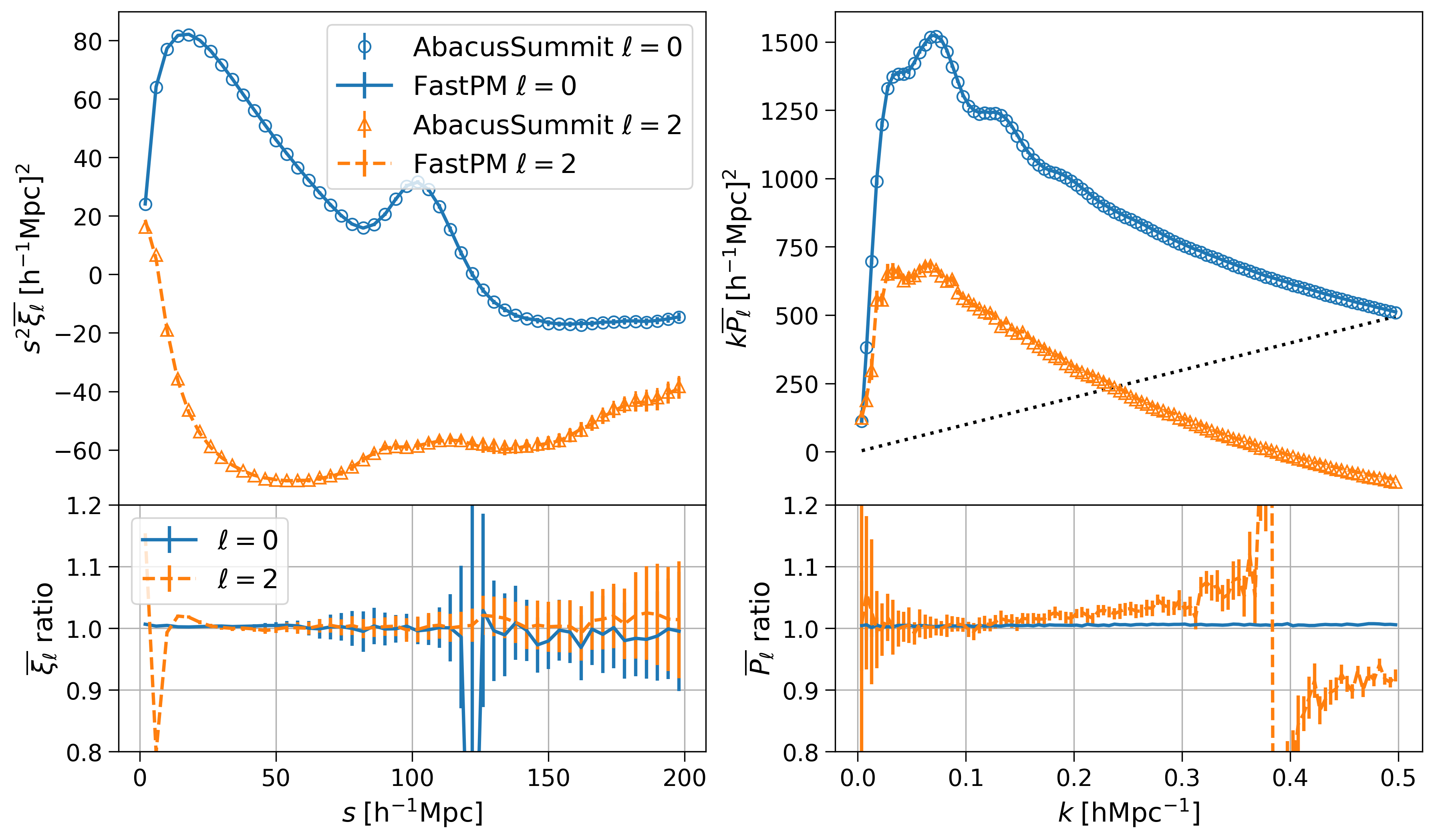
Figure 2: Comparison of the mean LRG power spectrum and correlation function multipoles from 25 AbacusSummit and FastPM paired simulations. The left and right panels are for the correlation function and power spectrum, respectively. The upper panels overplot the monopoles ($\ell=0$) and quadrupoles ($\ell=2$) from the two simulations. The circular and triangular points denote the AbacusSummit monopoles and quadrupoles, respectively. Correspondingly, the solid and dashed lines show the monopoles and quadrupoles from FastPM, respectively. The black dotted line denotes the mean Poisson shot noise from FastPM, which closely matches to the AbacusSummit one with $0.3$ per cent difference. The lower panels display the ratios of the mean monopoles and quadrupoles between FastPM and AbacusSummit. Note that some large fluctuations shown are simply due to the zero crossings of the signals. Overall, the agreement is good on the two-point clustering between the two catalogs.

With the best-fit HOD parameters, we populate galaxies into FastPM halo catalogs over 25 realizations. As an example, here we display the FastPM LRG clustering. Figure 2 displays the comparison of the mean two-point galaxy clustering from AbacusSummit and FastPM LRG catalogs averaged over 25 realizations. The left and right panels are for the correlation function and power spectrum multipoles, respectively. The upper panels show the overall shape of the monopole ($\ell=0$) and quadrupole ($\ell=2$) moments from the two simulations. The error bars represent the standard deviation of the mean. The power spectrum monopoles shown have been subtracted by the Poisson shot noise. We denote the mean shot noise of the FastPM catalogs as the black dotted line in the upper right panel. The mean galaxy number density of FastPM is closely matched the AbacusSummit one with only $0.3$ per cent difference. The lower panels show the ratios of the monopoles and quadrupoles between FastPM and AbacusSummit, respectively. With the HOD parameters fitted from $500\,h^{-1}\mathrm{Mpc}$ sub-boxes, we can match the FastPM monopoles to the AbacusSummit ones with $\sim 1$ per cent level for both Fourier and configuration spaces. In terms of the power spectrum quadrupoles, the difference is within 2 (5) per cent up-to $k=0.2\,h\,\mathrm{Mpc}^{-1}$ ($k=0.3\,h\,\mathrm{Mpc}^{-1}$), and within 10 per cent up-to $k=0.5\,h\,\mathrm{Mpc}^{-1}$. For the correlation function quadrupoles, the agreement is also within 1 per cent level except for scales $s<25\,h^{-1}\mathrm{Mpc}$. Note that the result we show here is conservative; we can further improve the agreement of the quadrupoles by turning HOD parameters. In figure 10 and 11, we show similar results for ELGs and QSOs, respectively.

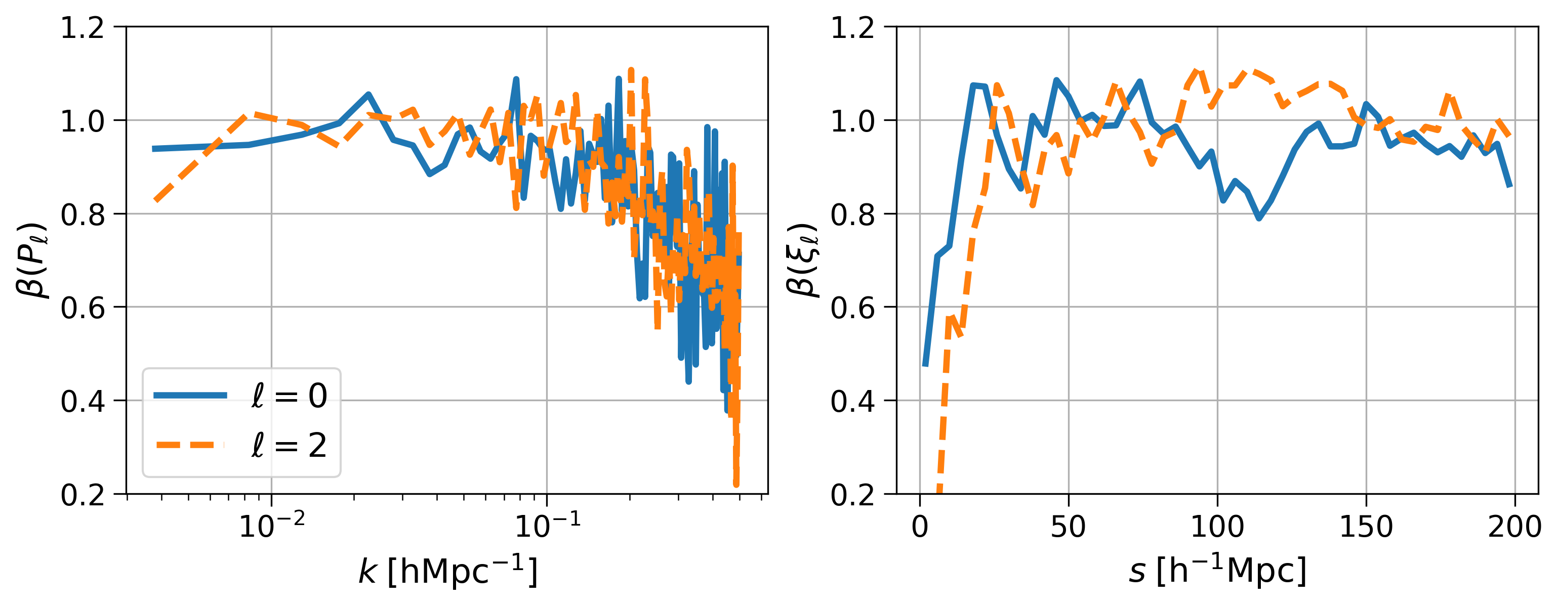
Figure 3: Diagonal terms of the $\beta^{\text{diag}}$ matrix for the LRG power spectrum and correlation function multipoles. The solid and dashed lines denote the monopole and quadrupole, respectively. $\beta$ is close to 1 at large scales, which indicates that there is high cross-correlation between the AbacusSummit and FastPM clustering.

Figure 3 illustrates the CARPool coefficient $\beta$ (see eq. 3.21) for both the LRG power spectrum multipoles (in the left panel) and correlation function multipoles (in the right panel). The solid and dashed lines are for the monopoles and quadrupoles, respectively. For the power spectrum, $\beta>0.8$ at $k<0.2\,h\,\mathrm{Mpc}^{-1}$, which indicates the high cross-correlation at large scales. Correspondingly, for the correlation function, $\beta>0.8$ for $s>25\,h^{-1}\mathrm{Mpc}$. There is relatively large difference on $\beta$ between the correlation function monopole and quadrupole around $s=100\,h^{-1}\mathrm{Mpc}$, which is probably due to statistical fluctuation. Since there is high cross-correlation between the neighbouring $s$ bins of $\text{Cov}(\xi^{\text{Abacus}}_{\ell},\,\xi^{\text{FastPM}}_{\ell})$, statistical fluctuation on the diagonal terms from the off-diagonal terms can be large.

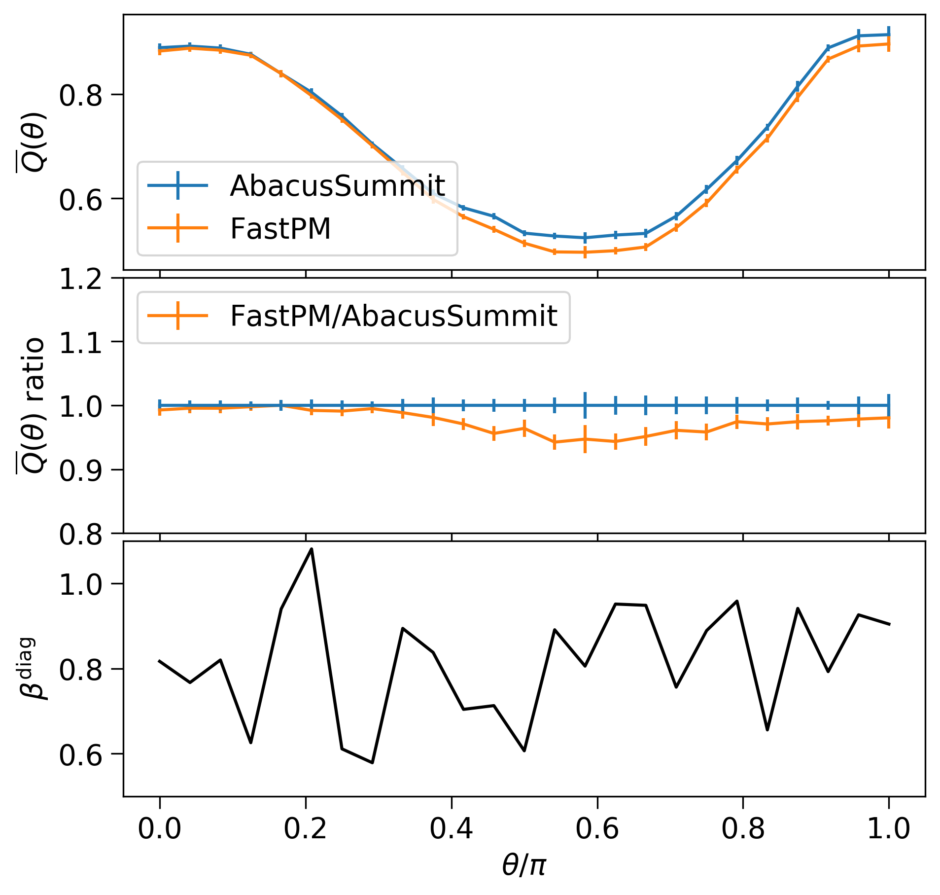
Figure 4: Upper panel: Comparison of the mean reduced bispectra $\overline{Q}(\theta)$ averaged over 25 paired AbacusSummit and FastPM LRG mocks. The triangle configurations of the bispectra are set as $k_{2}=2k_{1}=0.2\,h\,\mathrm{Mpc}^{-1}$ with $\theta$ as the subtended angle between the wave vectors ${\bf\it k_{1}}$ and ${\bf\it k_{2}}$. Middle panel: Ratio of $\overline{Q}(\theta)$ between FastPM and AbacusSummit. Lower panel: $\beta^{\text{diag}}$ coefficient for the paired AbacusSummit and FastPM LRG mocks with $\beta\simeq 0.8$ for such configuration.

In addition, we check the relative difference of the bispectra between the AbacusSummit and FastPM LRGs. In figure 4, we specifically compare the bispectra from the triangle configurations of $k_{2}=2k_{1}=0.2\,h\,\mathrm{Mpc}^{-1}$. The upper panel shows the mean reduced bispectra $\overline{Q}(\theta)$ (calculated via eq. 4.8). The middle panel shows the ratio of $\overline{Q}(\theta)$ between FastPM and AbacusSummit. The agreement is within 5 per cent, which is consistent with the finding in [64]. The lower panel shows the coefficient $\beta$, which is around $0.8$, indicating the relatively high cross-correlation between the bispectra from the AbacusSummit and FastPM LRGs at these configurations.

5.2 Suppressing the sample variance of galaxy clustering

In this section, we illustrate the suppression on the sample variance of galaxy clustering from CARPool.

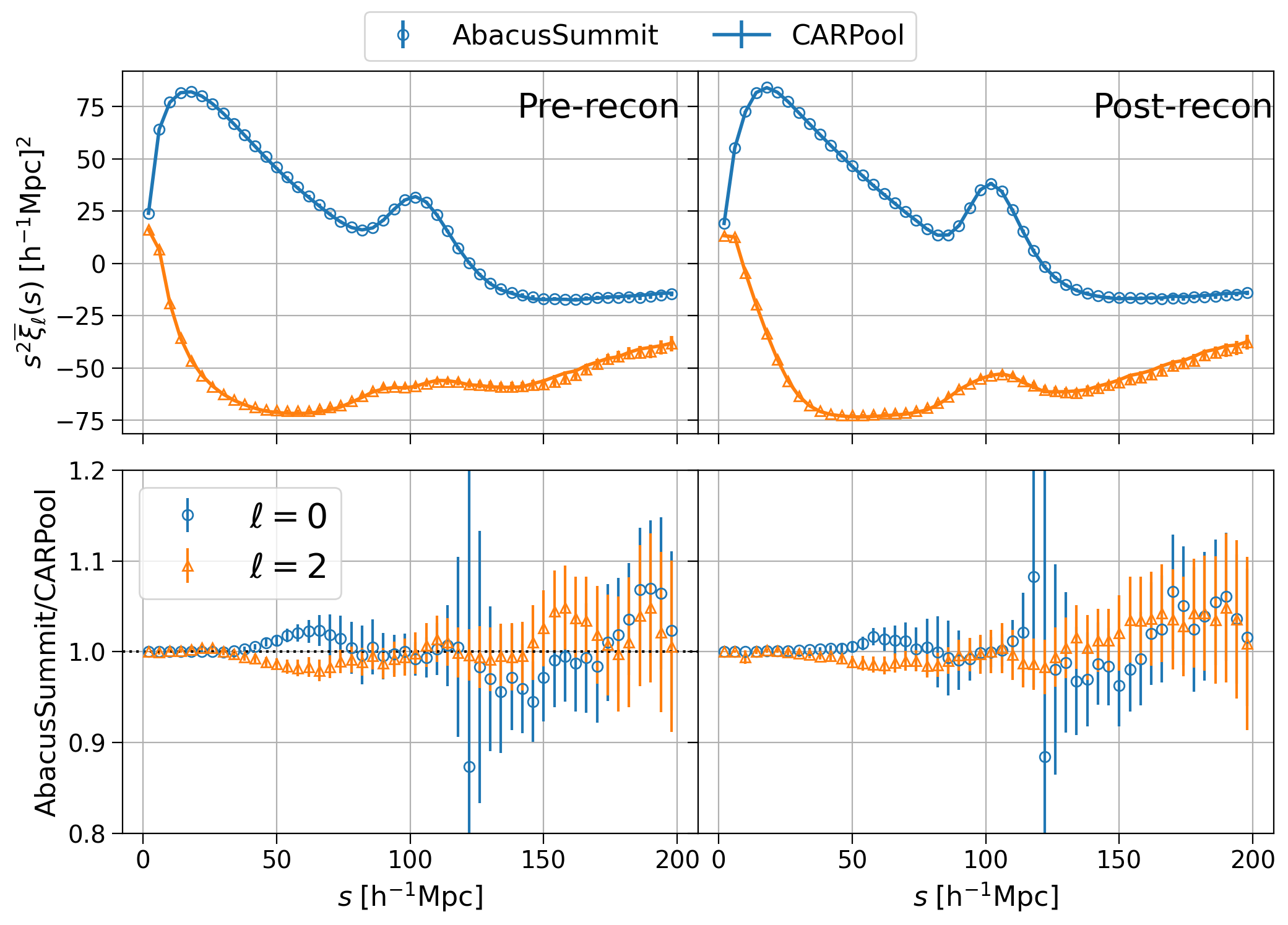
Figure 5: Upper panels: Comparison of the correlation function multipoles after CARPool applied with those from the original AbacusSummit LRG catalogs. We show the mean over 25 realizations. The markers denote the results from AbacusSummit with the circles for $\xi_{0}$ and the triangles for $\xi_{2}$. Correspondingly, the solid lines are the CARPool results. Lower panels: Ratio of the correlation function multipoles before and after CARPool applied. The left and right panels display the results before and after the BAO reconstruction, respectively.

Figure 5 compares the correlation function multipoles ($\ell=0$ and $\ell=2$) from the AbacusSummit LRGs before and after CARPool applied. The left and right panels show the results before and after the BAO reconstruction, respectively. In the upper panels, the data points represent the overall shape of the mean correlation function monopole (circular points) and quadrupole (triangular points) averaged over 25 AbacusSummit catalogs, and the lines denote the results with CARPool applied. The error bars represent $1\sigma$ error of the mean. In the lower panels, we show the ratios of the mean multipoles before and after CARPool applied. The ratios are close to $1.0$ with the fluctuation within $\sim 2\sigma$ level, indicating that the mean signal from CARPool is unbiased compared to the original AbacusSummit result for both the pre- and post-reconstruction cases. Note that the large fluctuation of the monopoles at around $120\,h^{-1}\mathrm{Mpc}$ is simply due to the zero crossing of the signal.

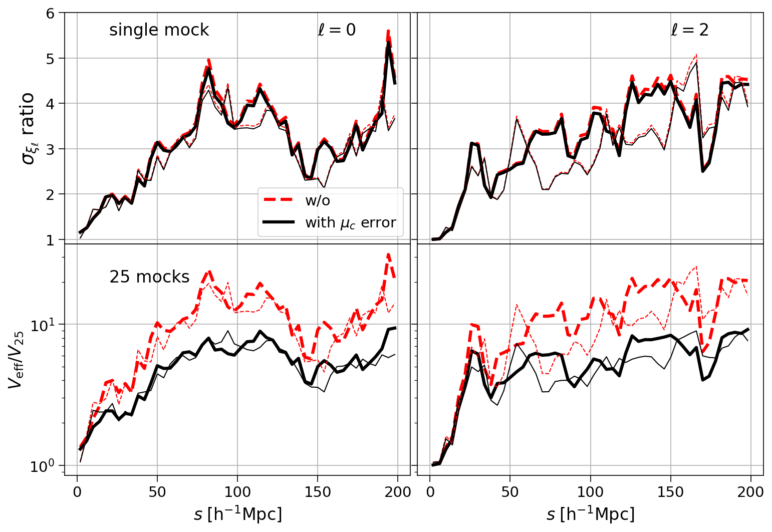
Figure 6: Upper panels: Reduction of the standard deviation of the correlation function multipoles from CARPool. We consider the standard deviation in terms of one single mock. Lower panels: Increase on the effective volume of 25 mocks from CARPool. The left and right panels are for the monopole and quadrupole, respectively. The black solid lines consider the error of $\mu_{c}$ in the CARPool result, while the red dashed lines do not, and represent the optimal gains. We compare the results before and after the BAO reconstruction, shown as the thick and thin lines, respectively.

Figure 6 illustrates the reduction on the sample variance of the AbacusSummit LRG catalogs from CARPool. The upper panels plot the ratios of the standard deviation of the AbacusSummit LRG correlation function multipoles before and after CARPool applied. We get the standard deviation from the diagonal terms of the correlation function covariance matrices. The left and right panels are for the monopole and quadrupole, respectively. With CARPool, the standard deviation of one single mock is reduced by a factor of $3\sim 4$ at the scale $50\,h^{-1}\mathrm{Mpc}<s<200\,h^{-1}\mathrm{Mpc}$. At $s<50\,h^{-1}\mathrm{Mpc}$, the reduction factor is less but still larger than 1, slightly better than that from the theoretical control variates, e.g. figure 7 of [49]. In the case that we consider the sample variance of $\mu_{c}$ (in eq. 3.14) estimated from the FastPM catalogs with random ICs, the result is shown as the black solid lines. Ignoring the $\mu_{c}$ error, we have the red dashed lines, which represent the optimal results. The difference between the black and red lines is small, indicating that the contribution of $\mu_{c}$ error is negligible on the sample variance in terms of one single mock. In addition, we compare the results before and after the BAO reconstruction, shown as the thick and thin lines, respectively. They have similar amplitude, indicating that the reconstruction does not affect much on the CARPool performance.

The lower panels of figure 6 show the increase on the volume over 25 mocks, denoted as $V_{25}$. We calculate it based on eq. 3.18, i.e. $V_{\text{eff}}/V_{25}=\sigma^{2}_{\overline{y}}/\sigma^{2}_{\overline{x}}$. Without the sample variance of $\mu_{c}$, we can increase the simulation volume a factor of $\sim 10$ at $50<s<200\,h^{-1}\mathrm{Mpc}$ from CARPool, shown as the dashed lines. Considering the $\mu_{c}$ error estimated from 313 FastPM catalogs, the gain is degraded to a factor of $\sim 5$. We expect that using the FastPM catalogs with the fixed-amplitude or fixed-and-paired ICs can effectively reduce the sample variance of $\mu_{c}$, and lift the solid lines closer to the dashed lines, similar to the case of halo clustering as studied in [45]. Figure 15 illustrates that we can reach about $80$ per cent of the optimal $V_{\text{eff}}$ in the case that we use 200 fixed-amplitude FastPM catalogs to estimate $\mu_{c}$.

Similar to figure 6, figure 7 shows the results for the AbacusSummit ELGs based on the power spectrum monopoles and quadrupoles. At $k<0.1\,h\,\mathrm{Mpc}^{-1}$, the reduction on the standard deviation of one single mock is larger than a factor of $2$, and the effective volume of 25 mocks increases about $4$ times. Such significant suppression on the sample variance at large scales can be beneficial for a tighter constraint on the theoretical systematics for BAO, RSD and $f_{\mathrm{nl}}$. We notice that the $\sigma$ ratio (or $V_{\text{eff}}/V_{25}$) before and after the BAO reconstruction varies less for the power spectrum case, compared to that of the correlation function (figure 6). It is probably due to the larger cross-correlation between the diagonal and off-diagonal terms in the correlation function covariance matrix.

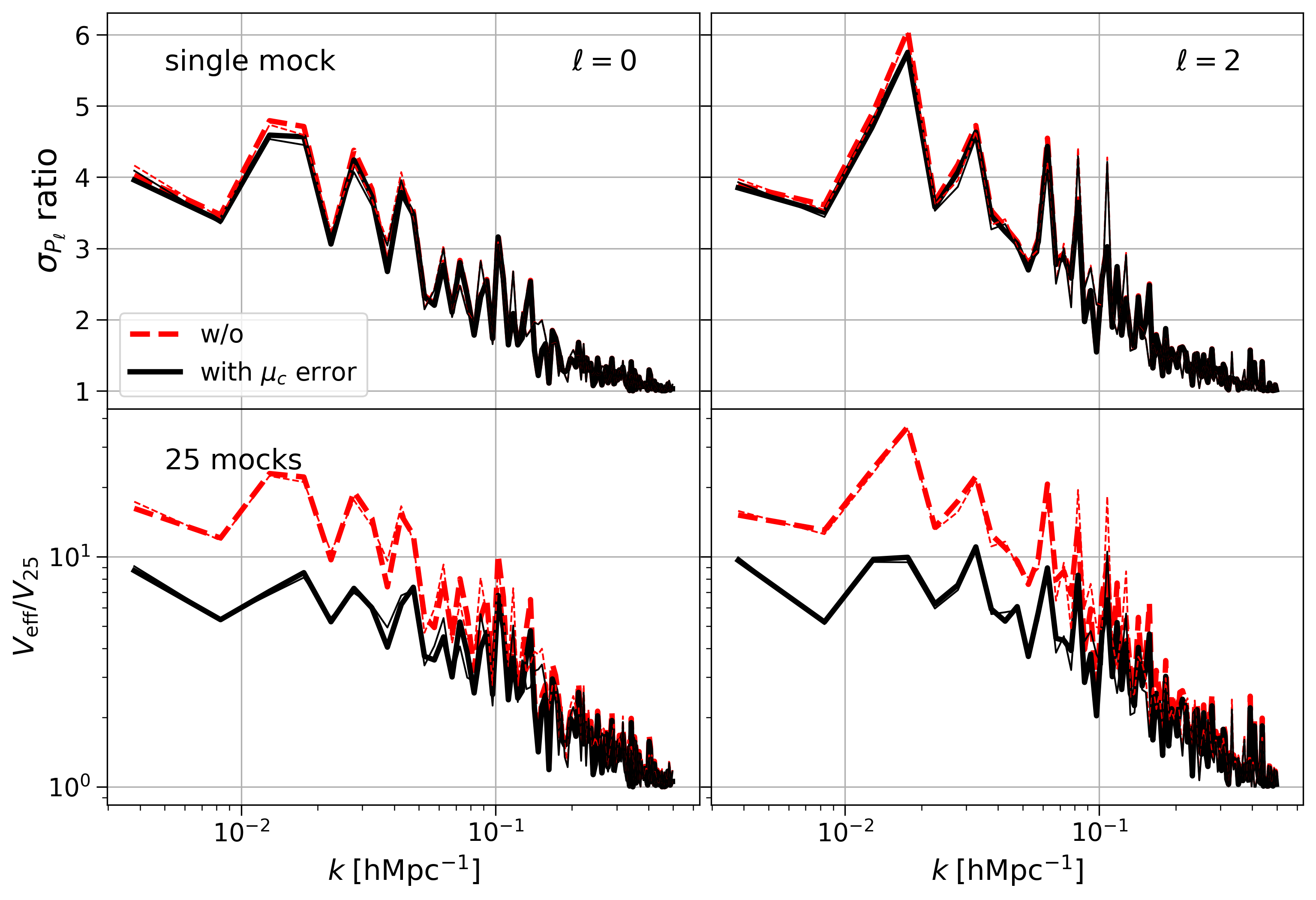
Figure 7: Similar to figure 6 but for the AbacusSummit ELG power spectrum multipoles.

Our previous study [45] has shown that CARPool can effectively reduce the sample variance of the halo bispectrum with the triangle configurations $k_{2}=2k_{1}=0.2\,h\,\mathrm{Mpc}^{-1}$. In this study, we further check that it is true for the galaxy bispectrum as well, as shown in figure 8. In the left panel, we check the ratio of the AbacusSummit LRG reduced bispectrum (eq. 4.8) before and after CARPool, shown as the squares. It fluctuates around $1.0$ without noticeable bias. The orange shaded region denotes the standard deviation of the result with CARPool. In the right panel, we display the ratio of the standard deviation before and after CARPool applied. The solid line is for the case of one single mock, and the dashed line is for the mean of 25 mocks. The CARPool method reduces the standard deviation by $\sim 1.6$ times for both cases.

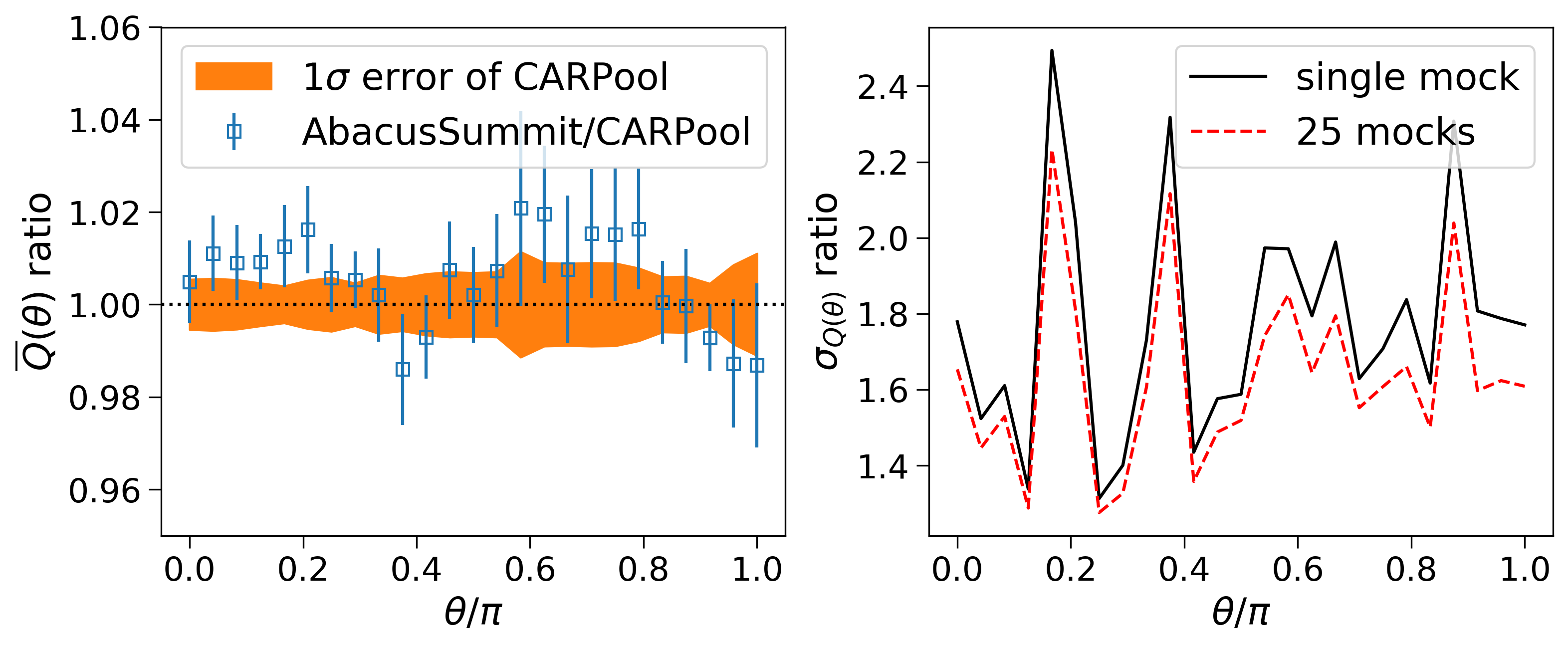
Figure 8: Left panel: Ratio of the mean $Q(\theta)$ of the AbacusSummit LRGs before and after CARPool applied shown as the blue squares. The error bars denote $1\sigma$ error of the mean, and the shaded region depicts the error bar after CARPool applied. Right panel: Ratio of the standard deviation of $Q(\theta)$ before and after CARPool. The black solid line is the case of one single mock, while the red dashed line represents for the mean of 25 mocks.

5.3 Improving the BAO constraints

We have shown that the sample variance of galaxy clustering can be effectively suppressed by CARPool. Such clustering with smaller sample variance can be useful to constrain theoretical systematics tighter, given a limited number of $N$-body simulations. Here we perform the BAO fitting as an example. We demonstrate that fitting the galaxy clustering with CARPool applied outputs unbiased result but with smaller uncertainties on the BAO scale parameters.

	$\langle\alpha\rangle$	$\sigma_{\alpha}$	$\langle\epsilon\rangle$	$\sigma_{\epsilon}$	$\langle\alpha_{\parallel}\rangle$	$\sigma_{\alpha_{\parallel}}$	$\langle\alpha_{\perp}\rangle$	$\sigma_{\alpha_{\perp}}$
	Pre-recon LRGs
Pre-CARPool	1.0039	0.0044	0.0031	0.0073	1.0104	0.0170	1.0008	0.0071
Post-CARPool	1.0046	0.0026	0.0016	0.0034	1.0078	0.0086	1.0031	0.0031
ratio		1.6835		2.1465		1.9815		2.3018
	Post-recon LRGs
Pre-CARPool	1.0000	0.0031	-0.0003	0.0048	0.9995	0.0105	1.0003	0.0052
Post-CARPool	1.0007	0.0020	0.0004	0.0026	1.0015	0.0063	1.0003	0.0024
ratio		1.5449		1.8516		1.6744		2.1344
	Pre-recon ELGs
Pre-CARPool	1.0031	0.0053	0.0022	0.0057	1.0075	0.0136	1.0010	0.0070
Post-CARPool	1.0030	0.0038	0.0032	0.0028	1.0094	0.0072	0.9998	0.0043
ratio		1.3958		2.0717		1.8693		1.6276
	Post-recon ELGs
Pre-CARPool	1.0015	0.0036	-0.0013	0.0026	0.9989	0.0066	1.0028	0.0042
Post-CARPool	1.0020	0.0027	-0.0002	0.0022	1.0017	0.0040	1.0022	0.0042
ratio		1.3317		1.1627		1.6616		1.0001

Table 2: Summary of the BAO scale parameters fitted from the AbacusSummit LRGs and ELGs two-point clustering before and after CARPool applied, denoted as Pre-CARPool and Post-CARPool, respectively. For each tracer, we also compare the results before and after the BAO reconstruction, denoted as Pre-recon and Post-recon, respectively.

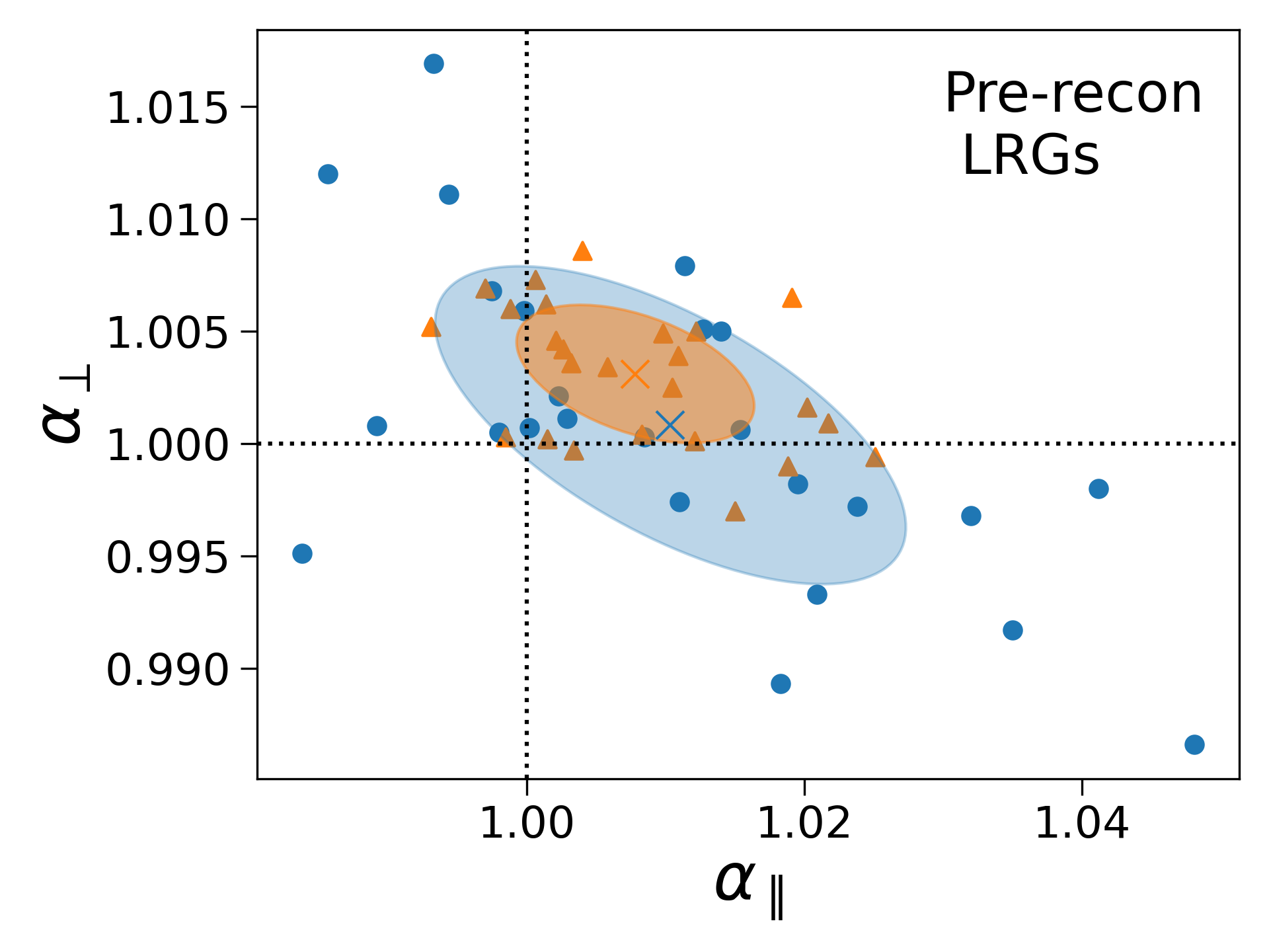
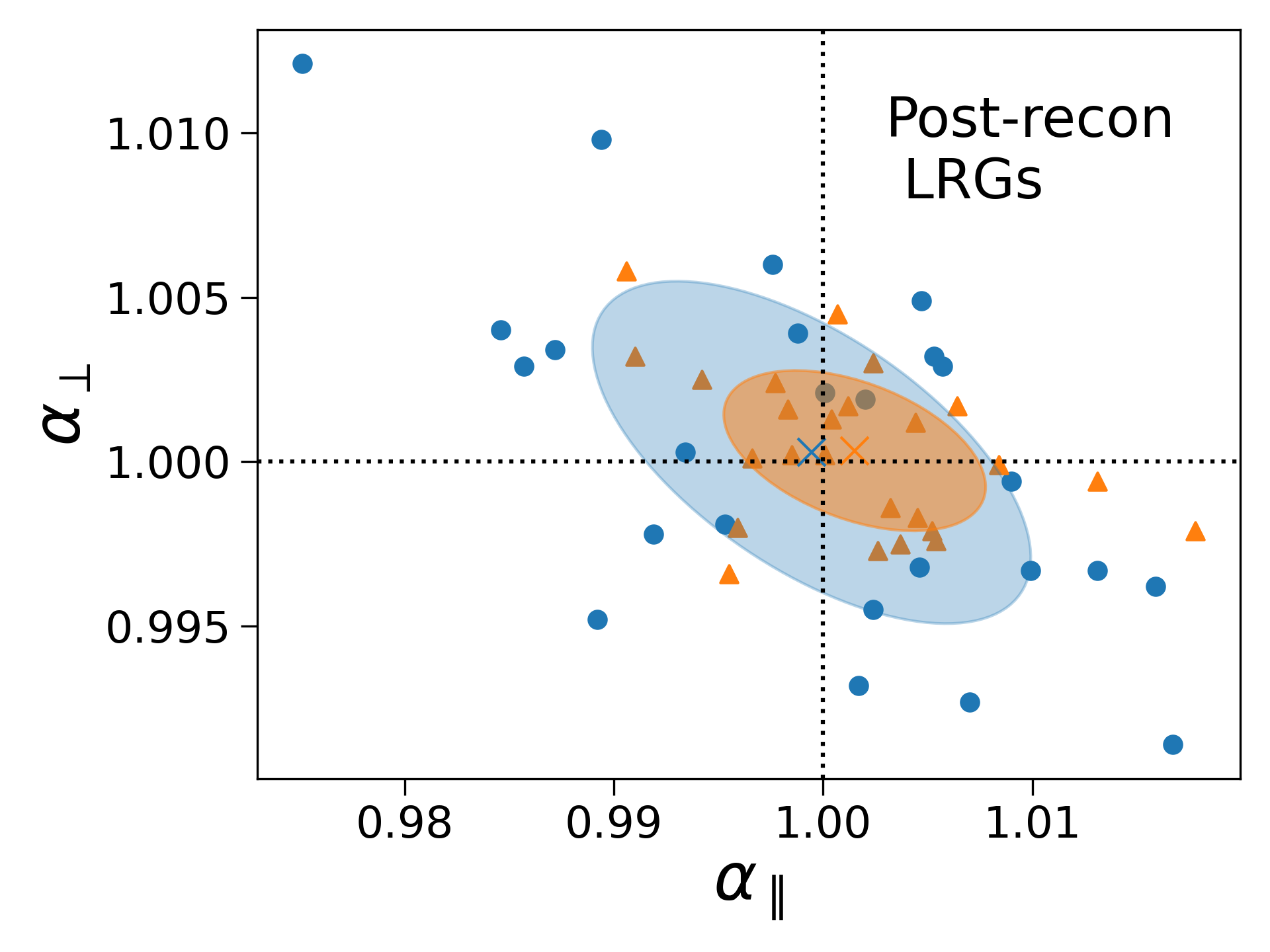
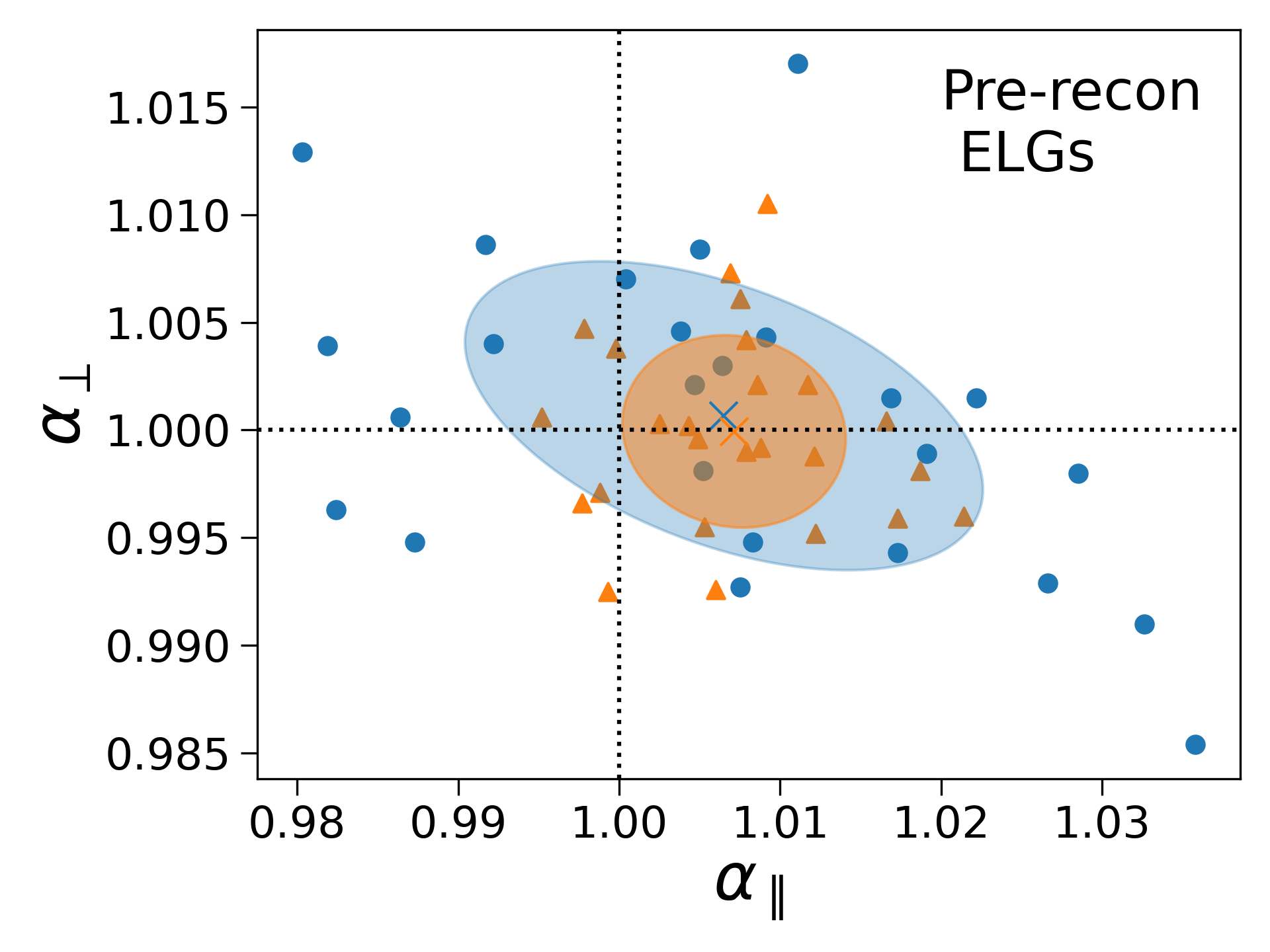
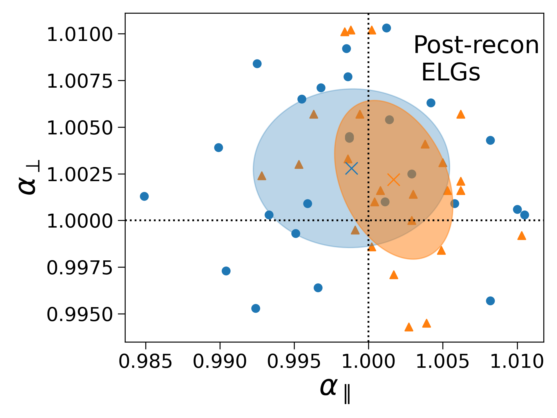
Figure 9: BAO fitting parameters $\alpha_{\parallel}$ and $\alpha_{\perp}$ fitted from the AbacusSummit LRGs and ELGs. The left and right panels show the results before and after the BAO reconstruction, respectively. For LRGs, we fit the correlation function monopole and quadrupole in the range $50\,h^{-1}\mathrm{Mpc}<s<150\,h^{-1}\mathrm{Mpc}$. For ELGs, we fit the power spectrum monopole and quadrupole in the range $0.02\,h\,\mathrm{Mpc}^{-1}<k<0.3\,h\,\mathrm{Mpc}^{-1}$. Each data point represents the fitting result from one mock. The blue and orange colors denote the results before and after CARPool applied, respectively. For each case, we plot a contour based on the mean (denoted by the crosses), the standard deviation, and the cross-correlation coefficient between $\alpha_{\parallel}$ and $\alpha_{\perp}$ over 25 realizations. With CARPool, the contour shrinks significantly, indicating the suppression on the sample variance of the BAO scale parameters over realizations.

In the fitting with barry, we set $\alpha$, $\epsilon$, $b_{0}$, $\beta$, $\Sigma_{\parallel}$, $\Sigma_{\perp}$, and $\Sigma_{s}$ as free parameters. We can convert $\alpha$ and $\epsilon$ to get $\alpha_{\parallel}$ and $\alpha_{\perp}$ based on eq. 4.13 and 4.16. We get the mean $\alpha$ and $\epsilon$ (or $\alpha_{\parallel}$ and $\alpha_{\perp}$) after marginalizing over the other parameters including the nuisance parameters. In figure 9, the upper panels show the marginalized mean of $\alpha_{\parallel}$ and $\alpha_{\perp}$ from fitting the correlation function monopoles and quadrupoles over 25 AbacusSummit LRG mocks. The left and right panels are the results before and after the BAO reconstruction, respectively. When we fit the clustering with and without CARPool applied, we use the same covariance matrix, which is estimated from 313 FastPM catalogs with the random ICs. Strictly speaking, the covariance matrix of the galaxy clustering after CARPool should be different from the one before CARPool (as shown in eq. 3.19). Here we only focus on the potential application of the CARPool method, and leave more details for future work. For the AbacusSummit clustering with reconstruction, we apply the same reconstruction process on the FastPM catalogs to obtain the post-reconstruction covariance matrix. In each panel, the blue circles and the orange triangles represent the results before and after CARPool applied, respectively. Each data point is fitted from one mock. To visually compare the scattering of the data points between the two cases, we plot two shaded contours, whose size and ellipticity are based on the standard deviations of $\alpha_{\parallel}$ and $\alpha_{\perp}$, as well as their cross-correlation coefficients. We match the colors of contours to those of data points. The mean values of $\alpha_{\parallel}$ and $\alpha_{\perp}$ are denoted by the crosses, which are close to each other from the two cases, indicating that there is little bias on the fitted parameters using the clustering with CARPool. Since the BAO reconstruction removes most of systematics from the non-linear structure growth and RSD, the resultant density field becomes more linear, and the BAO scale parameters are closer to 1. As shown in the right panel, the mean values of $\alpha_{\parallel}$ and $\alpha_{\perp}$ (shown as the crosses) are close to 1 for both cases before and after CARPool applied.

Similarly, we show the fitting results of the AbacusSummit ELGs in the lower panels of figure 9. We fit the power spectrum monopoles and quadrupoles over 25 realizations. The results are similar to those of LRGs, illustrating that we can apply galaxy clustering with CARPool in both configuration and Fourier spaces for systematics study. We notice that there is a larger bias ($\sim 0.25\%$) on the mean $\alpha_{\perp}$ of post-reconstruction for both cases before and after CARPool applied compared to that of LRGs, indicating some systematic error. We have tested changing the density smoothing parameter from $10\,h^{-1}\mathrm{Mpc}$ to $15\,h^{-1}\mathrm{Mpc}$, which is a parameter can be optimized [101, 102] for the BAO reconstruction, however, it reduce the bias little. Increasing the random sample size from 5 to 20 times of the data size does not help neither, when we perform reconstruction for the AbacusSummit ELGs. We suspect that the systematics can be caused by the covariance matrix from the limited number of FastPM realizations. If we replace our covariance matrix by the one from 1000 realizations of EZmocks[103], the bias can be largely mitigated. We discuss the result in appendix D. In terms of the dispersions of the BAO fitting parameters among 25 AbacusSummit mocks, we have checked that our results agree well with the ones from the studies of the LRG and ELG HOD systematics [104, 105]. In their studies, the “FirstGen” mocks are the same as our AbacusSummit mocks.

Table 2 lists the quantitative values of the BAO fitting parameters for the AbacusSummit LRGs and ELGs, respectively. In the first few columns, we show the mean of $\alpha$ and $\epsilon$ over 25 mocks, as well as their standard deviation, i.e. $\sigma_{\alpha}$ and $\sigma_{\epsilon}$. In the last few columns, we show the mean and standard deviation of $\alpha_{\parallel}$ and $\alpha_{\perp}$, respectively. In addition, we display the ratio of the mean and standard deviation before and after CARPool applied (denoted as Pre-CARPool and Post-CARPool). For the mean values of the parameters, we expect that their ratios are close to 1, which is the case except for $\epsilon$. It is simply due to numerical fluctuation, since $\epsilon$ is close to 0 especially for the post-reconstruction. If we take the difference between $\epsilon$ from Pre- and Post-CARPool, it is less than or comparable with the standard deviation of the mean, i.e. $\sigma_{\epsilon}/\sqrt{25}$. For the ratio of the standard deviation before and after CARPool, we see that it is larger than 1. For the LRGs after the reconstruction, the constraints on $\alpha$, $\epsilon$, $\alpha_{\parallel}$ and $\alpha_{\perp}$ are enhanced from CARPool by a factor of 1.54, 1.85, 1.67, and 2.13, respectively. For the ELGs after the reconstruction, the improved factors are 1.33, 1.16, 1.66, and 1.0, respectively. Our result is generally consistent with that from the theoretical control variates [49, 104, 105], the relative difference can be caused by different settings on the reconstruction and BAO fitting.

6 Conclusions and discussions

To study the CARPool performance on galaxy clustering, we utilize the FastPM simulations, which use the same cosmology as the AbacusSummit simulations. Based on the HOD models, we produce the FastPM galaxy catalogs, which can mimic the DESI-like LRGs, ELGs, and QSOs from AbacusSummit. For each tracer, the FastPM galaxy number density and the two-point clustering are well matched to those of AbacusSummit. The agreement is within a few per cent or better for both the correlation function and power spectrum multipoles at the scales relating to the BAO and RSD analyses. Although the higher-order galaxy clustering is not included in the HOD fitting, the resultant FastPM galaxy bispectrum agrees well with the AbacusSummit one. For LRGs, the agreement is better than $5$ per cent at the triangle configurations with $k_{2}=2k_{1}=0.2\,h\,\mathrm{Mpc}^{-1}$.

In addition, we utilize the paired FastPM and AbacusSummit simulations with the same ICs. There is high cross-correlation between the galaxy clustering from the two sets of simulations, which encourages the application of CARPool. In our previous study, we have shown that CARPool can effectively reduce the sample variance of AbacusSummit halo clustering [45]. In this work, we adopt the same methodology but extend it to the galaxy clustering. We have examined in detail that the galaxy clustering with CARPool applied is unbiased. We obtain the quantitative amount of the sample variance reduction from CARPool. Specifically, for the AbacusSummit LRG correlation function multipoles, we can reduce the standard deviation of a single mock by a factor of $3\sim 4$ at the scale range $50\,h^{-1}\mathrm{Mpc}<s<200\,h^{-1}\mathrm{Mpc}$. The effective volume of 25 mocks can be increased at least by a factor of 5 given the current number of FastPM simulations with random ICs. We expect that the optimal performance is a factor of $\sim 10$. It can be largely achieved with the assistance of the fixed-amplitude FastPM simulations, which can significantly reduce the sample variance of the ensemble average of the statistics, i.e. $\mu_{c}$ in eq. (3.14). For the power spectra of ELGs, we find that CARPool can increase the effective volume larger than 4 times at $k<0.1\,h\,\mathrm{Mpc}^{-1}$. We have checked the CARPool performance for the galaxy clustering after the BAO reconstruction applied. We show that there is no obvious difference on the cross-correlation coefficient (i.e. $\beta$) between the AbacusSummit and FastPM galaxy clustering before and after the BAO reconstruction.

For QSOs, we find that the cross-correlation coefficient of the two-point clustering is less than 1.0 between FastPM and AbacusSummit at large scales. We notice that the work [47] based on the Zel’dovich control variates has found similar result (see their figure 8). It is probably due to the high shot noise over all relevant scales that degrades the cross-correlation.

As a case of application, we study the improvement on the BAO constraints from the galaxy clustering with CARPool applied. We perform the BAO fitting on the AbacusSummit two-point galaxy clustering. For LRGs, we fit the correlation function monopole and quadrupole from each realization. We study the mean and standard deviation of the fitted BAO scale shifting parameters along and perpendicular to the LoS, i.e. $\alpha_{\parallel}$ and $\alpha_{\perp}$, which are related with the isotropic and anisotropic parameters, i.e. $\alpha$ and $\epsilon$. The mean of the fitted BAO scale parameters are close to each other before and after CARPool, illustrating that there is no bias from CARPool. The standard deviation is significantly reduced after CARPool applied. The reduction factors for $\alpha$, $\epsilon$, $\alpha_{\parallel}$ and $\alpha_{\perp}$ are respectively 1.54, 1.85, 1.67, and 2.13 for the case after the BAO reconstruction. For ELGs, we perform the BAO fitting similarly but on the power spectrum monopoles and quadrupoles. The improved factors of the constraints on $\alpha$, $\epsilon$, $\alpha_{\parallel}$ and $\alpha_{\perp}$ are 1.33, 1.16, 1.66, and 1.0, respectively.

Since the suppression on the sample variance is mostly significant at large scales, we expect that our work can be useful for tighter constraints on the theoretical systematics of the RSD and $f_{\mathrm{nl}}$ models as well. With some observational systematics, such as the imaging weight and fiber assignment, added on the galaxy catalogs, we are able to study their impacts on the clustering signal and the fitted cosmological parameters more precisely with the assistance of CARPool. We leave such study in future work.

Compared with the method of theoretical control variates, the main caveat of CARPool is computational time consuming. It takes tens of millions of CPU hours to generate hundreds of fast simulations in our case. To mitigate such issue, we may choose some cheaper simulations, such as EZmock [103, 106]. On the other hand, we usually run a large number of fast simulations to estimate covariance matrices for galaxy clustering analysis. If these fast simulations are ready, it can be a byproduct to perform CARPool. Although It is relatively cheap to fit HOD parameters for FastPM galaxies, performing density field reconstruction and calculating two-point statistics can take some amount of computational time for hundreds of galaxy mocks. Again, these products are not only used by CARPool, but can be useful for other purposes. In addition, it is straightforward to apply CARPool on higher order statistics, such as bispectrum, compared to the current stage of theoretical control variates.

Data availability.

We share all the necessary data and code to generate the figures and tables of this publication in zenodo repository https://zenodo.org/records/10644109.

Appendix A FastPM HOD parameters

	LRGs		ELGs		QSOs
Parameters	prior	best-fit	prior	best-fit	prior	best-fit
log$M_{\text{cut}}$	(11.6, 13.6)	12.69 [12.687]	(10.7, 13.0)	11.03 [11.22]	(11.6, 13.6)	13.25 [12.473]
log$M_{1}$	(9.0, 14.0)	11.71 [13.71]	(12.0, 15.0)	14.38 [12.28]	(9.0, 14.0)	11.88 [14.0]
$\sigma_{\text{log}M_{h}}$	(0.0, 4.0)	0.44 [0.5]	(0.0, 5.0)	1.12 [0.6]	(0.0, 4.0)	1.71 [1.0]
$\kappa$	(0.0, 20.0)	4.08 [1.0]	(0.5, 2.0)	2.32 [0.01]	(0.0, 20.0)	3.56 [1.0]
$\alpha$	(0.0, 1.3)	0.12 [0.8]	(0.0, 5.0)	0.49 [0.007]	(0.0, 1.3)	0.0455 [1.0]
$v_{\text{disp}}$	(0.7, 1.5)	1.01	(0.8, 1.6)	1.32	(0.7, 1.5)	0.58
$\gamma$			(5.0, 10.0)	6.28 [4.7]
$A$			(0.0, 1.0)	0.14
$p_{\text{max}}$				[0.65]	(0.0, 1.0)	0.20 [0.1]

Table 3: The priors and best-fits of the HOD parameters for the FastPM LRGs, ELGs, and QSOs, respectively. The HOD models vary for different tracers. We also show the corresponding HOD parameters of the AbacusSummit catalogs as the numbers in the square brackets.

Based on the HOD fitting process described in section 3.1, we obtain the best-fit HOD parameters for the FastPM galaxy catalogs, including LRGs, ELGs and QSOs, as shown in table 3. We also show the priors of the fitting parameters for each model. Different tracers have different HOD models. Each blank space indicates that there is no such parameter in a specific HOD model. Note that there are significant differences on halo properties between the FastPM and AbacusSummit catalogs, such as halo mass function, we should not expect the fitted FastPM HOD parameters close to those of AbacusSummit, even though we match the FastPM galaxy number density and two-point clustering at relatively large scales very well to those of AbacusSummit. The FastPM HOD parameters do not have similar physical interpretation as the ones from normal $N$-body simulations.

Appendix B FastPM ELG and QSO clustering

With the best-fit HOD parameters (in table 3) for the FastPM ELGs and QSOs, we compare their two-point clustering with those of AbacusSummit, as shown in figure 10 and figure 11. Same as figure 2, we display the mean over 25 catalogs. For QSOs, due to the low number density and large shot noise, the clustering signals are much noisier compared to those of LRGs and ELGs, shown as the larger fluctuation in the signal ratio.

In figure 12, we also show the $\beta$ coefficients of the correlation function and power spectrum multipoles. The upper panels are for ELGs, and the lower panels are for QSOs. The $\beta$ value of QSOs is smaller than that of ELGs or LRGs, which we suspect is mainly due to the large shot noise.

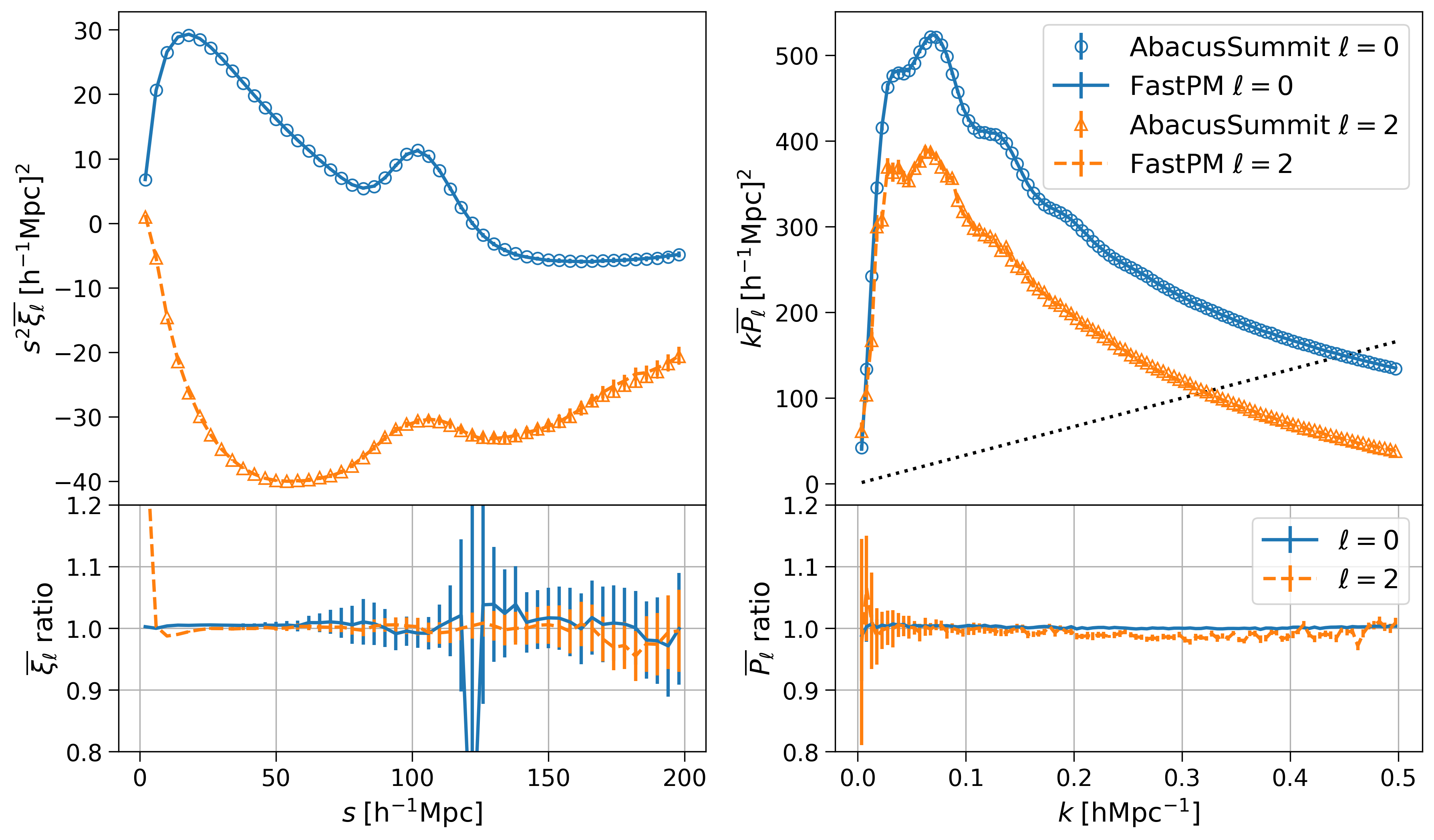
Figure 10: Same as figure 2 but for the comparison of the ELG clustering from AbacusSummit and FastPM.

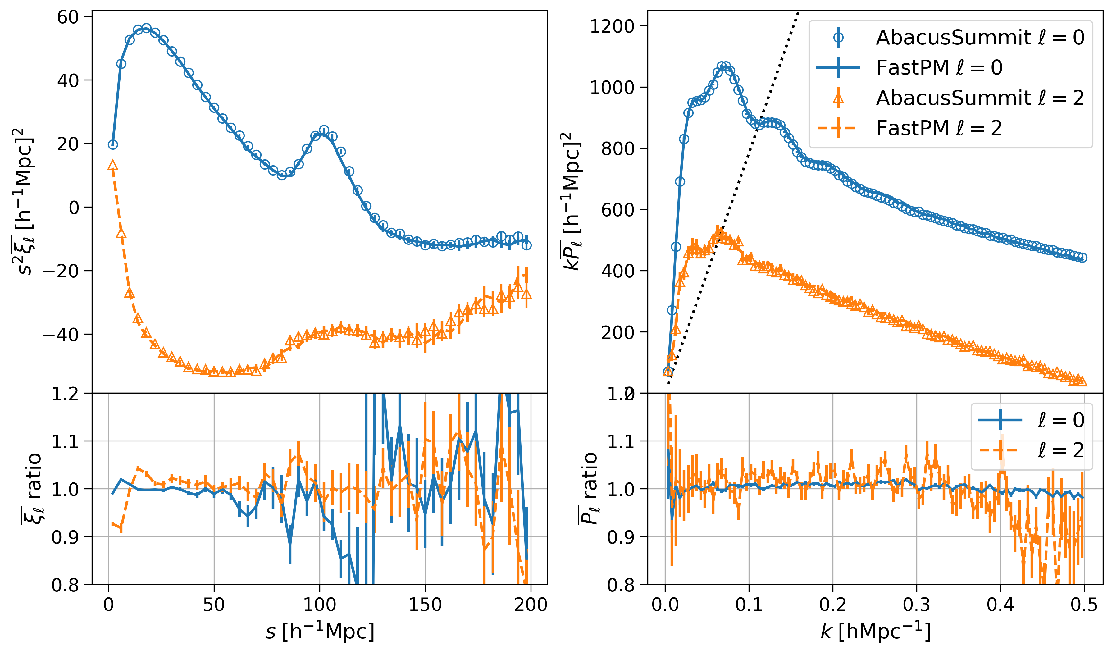
Figure 11: Same as figure 2 but for the comparison of the QSO clustering from AbacusSummit and FastPM.

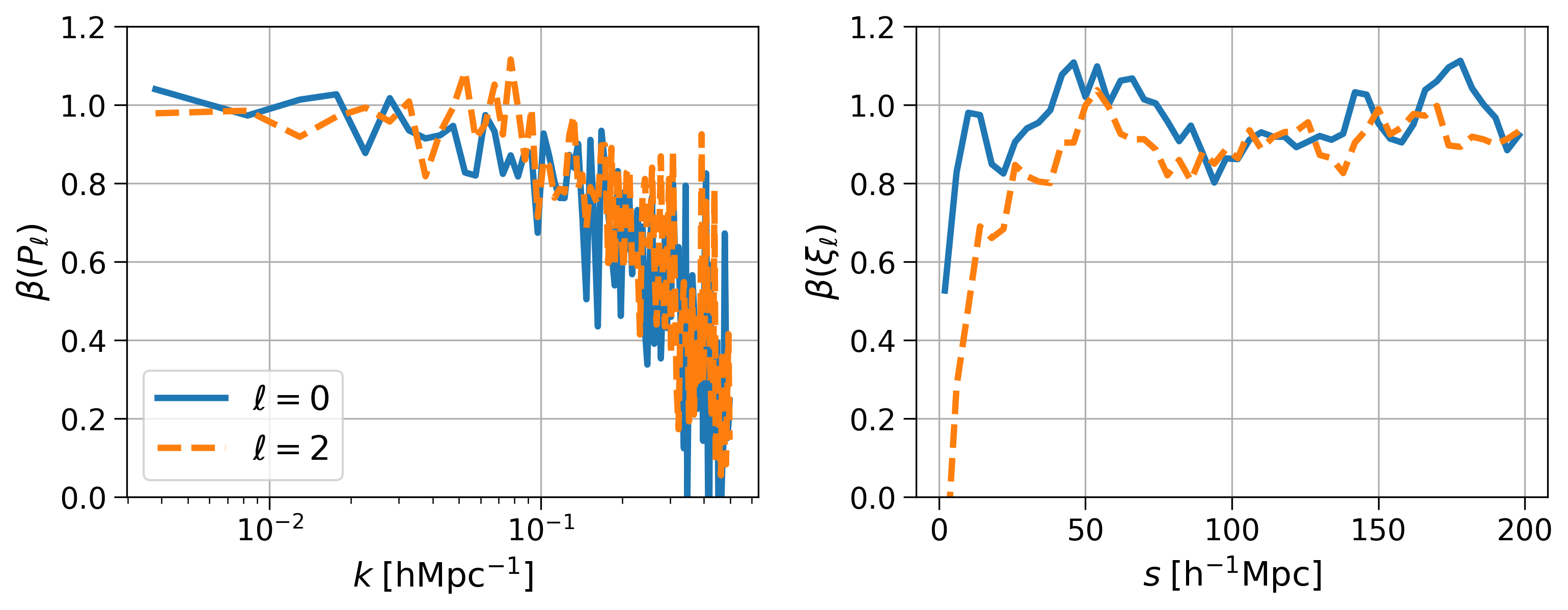
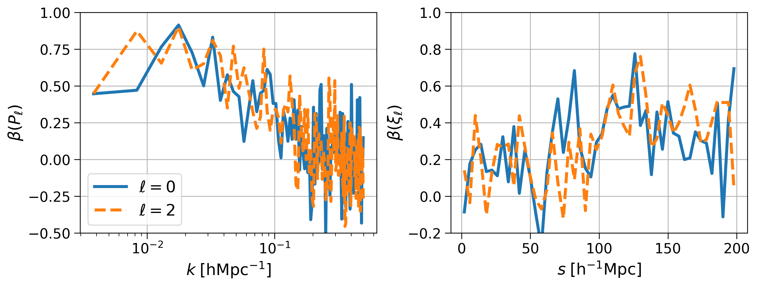
Figure 12: Similar to figure 3, we show the $\beta$ coefficients for the ELG and QSO clustering in the upper and lower panels, respectively.

Appendix C BAO parameters $\alpha$ and $\epsilon$

For complementary information, figure 13 displays the isotropic and anisotropic BAO scale parameters $\alpha$ and $\epsilon$ for LRGs and ELGs over 25 realizations, respectively. We focus on the results after the BAO reconstruction.

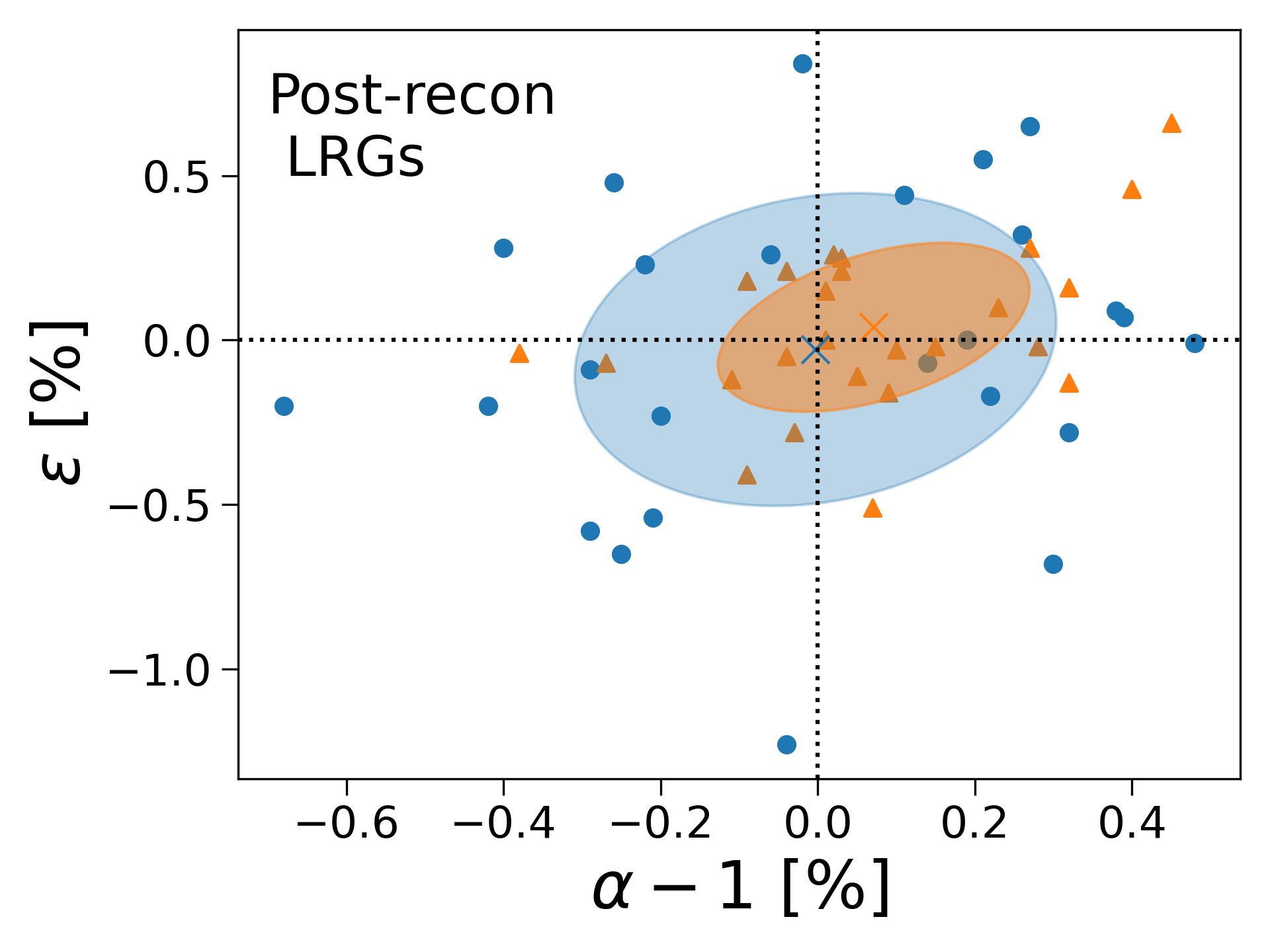
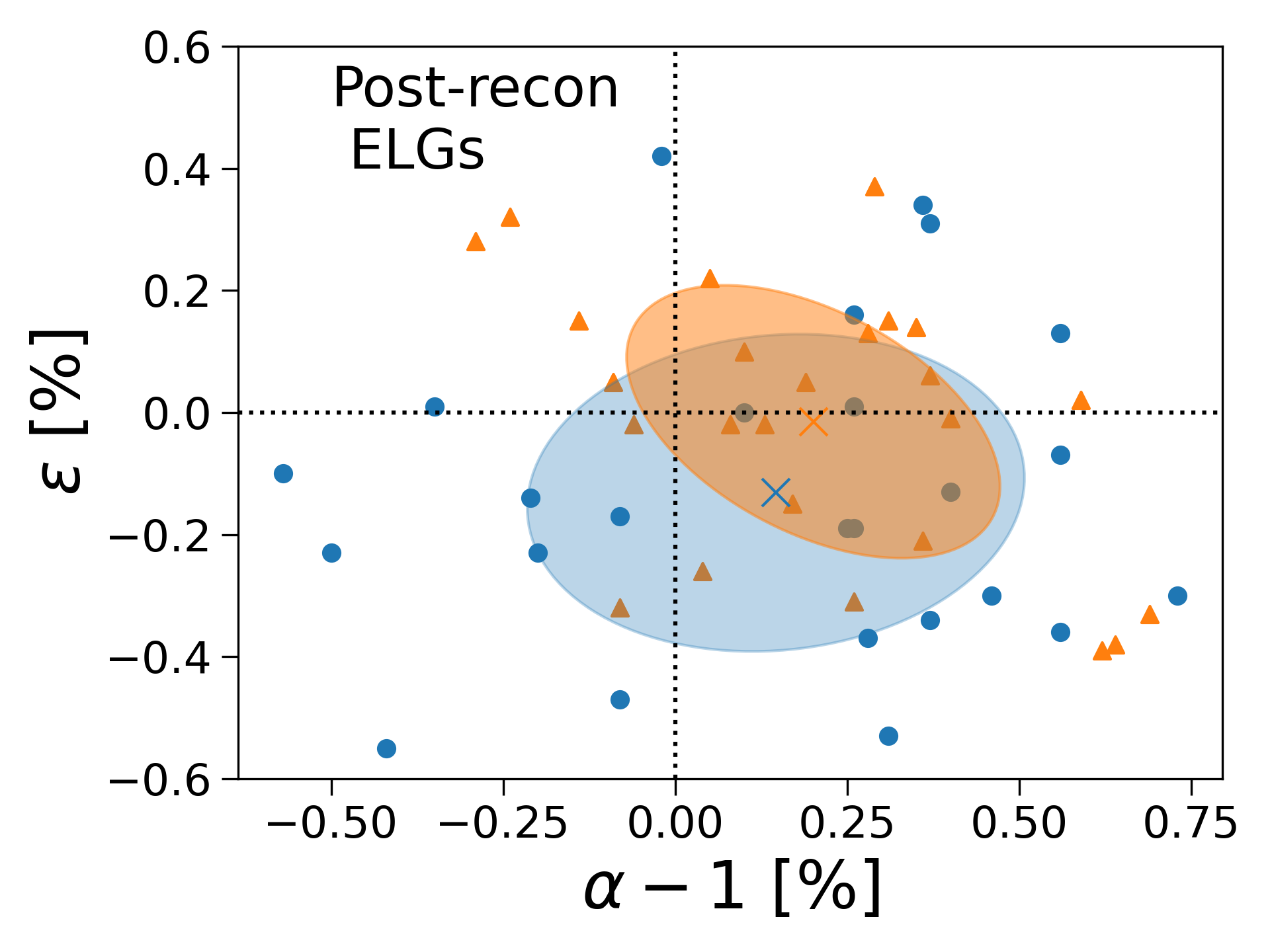
Figure 13: Similar to figure 9 but for the fitting parameters $\alpha$ and $\epsilon$ (eq. 4.15 and 4.16). The left and right panels are for LRGs and ELGs, respectively. Both are after the BAO reconstruction.

Appendix D ELG BAO fitting with the EZmock covariance

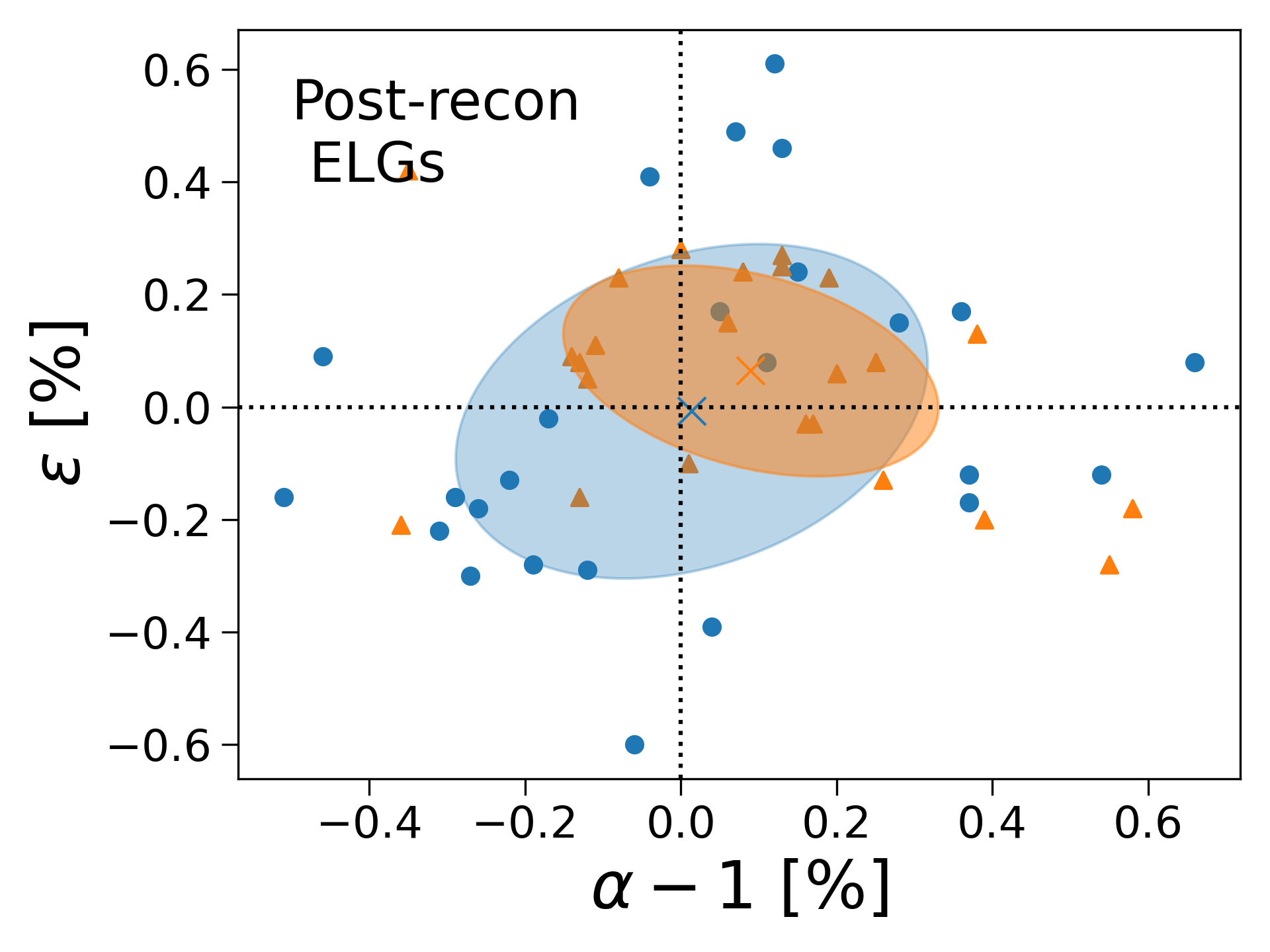
Figure 14: With the covariance matrix from EZmocks, we show the BAO fitting parameters for ELGs after the BAO reconstruction. The left (right) panel depicts the parameters $\alpha_{\parallel}$ and $\alpha_{\perp}$ ($\alpha$ and $\epsilon$).

From the lower right panel of figure 9, we notice that there is some bias on the BAO fitting parameter $\alpha_{\parallel}$ for ELGs after the BAO reconstruction. We suspect that the systematics can be due to the FastPM covariance matrix, which is estimated from a limited number (313) of FastPM realizations. If we replace the covariance matrix by the one from 1000 EZmocks, which is adopted in recent studies [49, 105], we can largely mitigate such systematics. We show the fitted BAO parameters in figure 14.

Appendix E Fixed-amplitude FastPM simulations

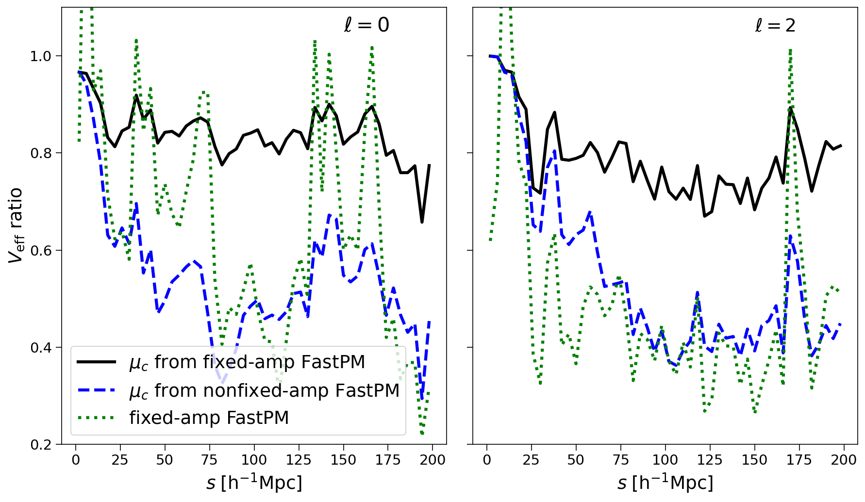
Figure 15: Influence of the $\mu_{c}$ error on the effective volume of 25 AbacusSummit LRG mocks from CARPool. We show the result for the correlation function monopole (left panel) and quadrupole (right panel). We consider the cases with $\mu_{c}$ estimated from a set of FastPM simulations with the nonfixed-amplitude and fixed-amplitude ICs, shown as the black solid and blue dashed lines, respectively. For each case, we calculate the ratio of the effective volume with respect to the optimal one with $\sigma^{2}_{\mu_{c}}=0$ (red lines in figure 6). In addition, we overplot the result if we use the fixed-amplitude FastPM simulations instead of CARPool to increase the effective volume, shown as the green dotted lines.

It has been studied that using the fixed-amplitude ICs can effectively suppress the sample variance of dark matter and halo clustering, e.g. [38, 45]. From the lower panels of figure 6 and 7, we have seen that the CARPool performance on the effective volume over multiple realizations depends on the sample variance of $\mu_{c}$, i.e. $\sigma^{2}_{\mu_{c}}$, which is estimated from a bunch of FastPM simulations in our study. We are interested in whether we can use the fixed-amplitude FastPM simulations to reduce the sample variance of galaxy clustering, hence, we can improve the CARPool performance.

In our previous work [45], we have generated more than $200$ fixed-amplitude FastPM halo catalogs. As an instance, we populate LRGs in the fixed-amplitude simulations adopting the same HOD parameters as the non-fixed-amplitude FastPM at $z=0.8$. We calculate the correlation function multipoles and the covariance matrix over 200 fixed-amplitude realizations. In figure 15, we compare the effective volumes of 25 AbacusSummit realizations from the cases with $\mu_{c}$ estimated from the default (non-fixed-amplitude) and fixed-amplitude FastPM simulations, respectively. Note that for the non-fixed-amplitude case, we use 313 realizations. To show the relative difference, we have rescaled the volumes by the reference, which is the optimal CARPool result with $\sigma^{2}_{\mu_{c}}=0$, i.e. assuming no sample variance on $\mu_{c}$. With smaller $\sigma_{\mu_{c}}$ from the fixed-amplitude FastPM, $V_{\text{eff}}$ increases significantly and reaches $\sim 80$ per cent of the optimal one. We also compare the volume of 25 fixed-amplitude FastPM LRGs with respect to the optimal CARPool result, shown as the green dotted lines. Interestingly, it is comparable with the CARPool result with $\mu_{c}$ from the non-fixed-amplitude FastPM. This test also demonstrates the power suppressing the sample variance via combining the fixed-amplitude and CARPool methods.

References

- [1] DESI Collaboration, A. Aghamousa, J. Aguilar, S. Ahlen, S. Alam, L.E. Allen et al., The DESI Experiment Part I: Science,Targeting, and Survey Design, arXiv e-prints (2016) arXiv:1611.00036 [1611.00036].
- [2] DESI Collaboration, A. Aghamousa, J. Aguilar, S. Ahlen, S. Alam, L.E. Allen et al., The DESI Experiment Part II: Instrument Design, arXiv e-prints (2016) arXiv:1611.00037 [1611.00037].
- [3] DESI Collaboration, B. Abareshi, J. Aguilar, S. Ahlen, S. Alam, D.M. Alexander et al., Overview of the Instrumentation for the Dark Energy Spectroscopic Instrument, AJ 164 (2022) 207 [2205.10939].
- [4] DESI Collaboration, A.G. Adame, J. Aguilar, S. Ahlen, S. Alam, G. Aldering et al., Validation of the Scientific Program for the Dark Energy Spectroscopic Instrument, arXiv e-prints (2023) arXiv:2306.06307 [2306.06307].
- [5] C. Hahn, M.J. Wilson, O. Ruiz-Macias, S. Cole, D.H. Weinberg, J. Moustakas et al., The DESI Bright Galaxy Survey: Final Target Selection, Design, and Validation, AJ 165 (2023) 253 [2208.08512].
- [6] R. Zhou, B. Dey, J.A. Newman, D.J. Eisenstein, K. Dawson, S. Bailey et al., Target Selection and Validation of DESI Luminous Red Galaxies, AJ 165 (2023) 58 [2208.08515].
- [7] A. Raichoor, J. Moustakas, J.A. Newman, T. Karim, S. Ahlen, S. Alam et al., Target Selection and Validation of DESI Emission Line Galaxies, AJ 165 (2023) 126 [2208.08513].
- [8] E. Chaussidon, C. Yèche, N. Palanque-Delabrouille, D.M. Alexander, J. Yang, S. Ahlen et al., Target Selection and Validation of DESI Quasars, ApJ 944 (2023) 107 [2208.08511].
- [9] S. Cole, W.J. Percival, J.A. Peacock, P. Norberg, C.M. Baugh, C.S. Frenk et al., The 2dF Galaxy Redshift Survey: power-spectrum analysis of the final data set and cosmological implications, MNRAS 362 (2005) 505 [astro-ph/0501174].
- [10] C. Blake, E.A. Kazin, F. Beutler, T.M. Davis, D. Parkinson, S. Brough et al., The WiggleZ Dark Energy Survey: mapping the distance-redshift relation with baryon acoustic oscillations, MNRAS 418 (2011) 1707 [1108.2635].
- [11] F. Beutler, C. Blake, M. Colless, D.H. Jones, L. Staveley-Smith, L. Campbell et al., The 6dF Galaxy Survey: baryon acoustic oscillations and the local Hubble constant, MNRAS 416 (2011) 3017 [1106.3366].
- [12] D.J. Eisenstein, I. Zehavi, D.W. Hogg, R. Scoccimarro, M.R. Blanton, R.C. Nichol et al., Detection of the Baryon Acoustic Peak in the Large-Scale Correlation Function of SDSS Luminous Red Galaxies, ApJ 633 (2005) 560 [astro-ph/0501171].
- [13] L. Anderson, É. Aubourg, S. Bailey, F. Beutler, V. Bhardwaj, M. Blanton et al., The clustering of galaxies in the SDSS-III Baryon Oscillation Spectroscopic Survey: baryon acoustic oscillations in the Data Releases 10 and 11 Galaxy samples, MNRAS 441 (2014) 24 [1312.4877].
- [14] F. Beutler, H.-J. Seo, A.J. Ross, P. McDonald, S. Saito, A.S. Bolton et al., The clustering of galaxies in the completed SDSS-III Baryon Oscillation Spectroscopic Survey: baryon acoustic oscillations in the Fourier space, MNRAS 464 (2017) 3409 [1607.03149].
- [15] J.E. Bautista, N.G. Busca, J. Guy, J. Rich, M. Blomqvist, H. du Mas des Bourboux et al., Measurement of baryon acoustic oscillation correlations at z = 2.3 with SDSS DR12 Ly-Forests, A & A 603 (2017) A12 [1702.00176].
- [16] H. du Mas des Bourboux, J. Rich, A. Font-Ribera, V. de Sainte Agathe, J. Farr, T. Etourneau et al., The Completed SDSS-IV Extended Baryon Oscillation Spectroscopic Survey: Baryon Acoustic Oscillations with Ly Forests, ApJ 901 (2020) 153 [2007.08995].
- [17] Y. Wang, G.-B. Zhao, C. Zhao, O.H.E. Philcox, S. Alam, A. Tamone et al., The clustering of the SDSS-IV extended baryon oscillation spectroscopic survey DR16 luminous red galaxy and emission-line galaxy samples: cosmic distance and structure growth measurements using multiple tracers in configuration space, MNRAS 498 (2020) 3470 [2007.09010].
- [18] G.-B. Zhao, Y. Wang, A. Taruya, W. Zhang, H. Gil-Marín, A. de Mattia et al., The completed SDSS-IV extended Baryon Oscillation Spectroscopic Survey: a multitracer analysis in Fourier space for measuring the cosmic structure growth and expansion rate, MNRAS 504 (2021) 33 [2007.09011].
- [19] N. Kaiser, Clustering in real space and in redshift space, MNRAS 227 (1987) 1.
- [20] A.J.S. Hamilton, Linear Redshift Distortions: a Review, in The Evolving Universe, D. Hamilton, ed., vol. 231 of Astrophysics and Space Science Library, p. 185, Jan., 1998, DOI [astro-ph/9708102].
- [21] F. Beutler, S. Saito, H.-J. Seo, J. Brinkmann, K.S. Dawson, D.J. Eisenstein et al., The clustering of galaxies in the SDSS-III Baryon Oscillation Spectroscopic Survey: testing gravity with redshift space distortions using the power spectrum multipoles, MNRAS 443 (2014) 1065 [1312.4611].
- [22] H. Gil-Marín, J.E. Bautista, R. Paviot, M. Vargas-Magaña, S. de la Torre, S. Fromenteau et al., The Completed SDSS-IV extended Baryon Oscillation Spectroscopic Survey: measurement of the BAO and growth rate of structure of the luminous red galaxy sample from the anisotropic power spectrum between redshifts 0.6 and 1.0, MNRAS 498 (2020) 2492 [2007.08994].
- [23] L. Verde, R. Jimenez, M. Kamionkowski and S. Matarrese, Tests for primordial non-Gaussianity, MNRAS 325 (2001) 412 [astro-ph/0011180].
- [24] R. Scoccimarro, E. Sefusatti and M. Zaldarriaga, Probing primordial non-Gaussianity with large-scale structure, Phys. Rev. D 69 (2004) 103513 [astro-ph/0312286].
- [25] N. Dalal, O. Doré, D. Huterer and A. Shirokov, Imprints of primordial non-Gaussianities on large-scale structure: Scale-dependent bias and abundance of virialized objects, Phys. Rev. D 77 (2008) 123514 [0710.4560].
- [26] E. Castorina, N. Hand, U. Seljak, F. Beutler, C.-H. Chuang, C. Zhao et al., Redshift-weighted constraints on primordial non-Gaussianity from the clustering of the eBOSS DR14 quasars in Fourier space, JCAP 2019 (2019) 010 [1904.08859].
- [27] E.-M. Mueller, M. Rezaie, W.J. Percival, A.J. Ross, R. Ruggeri, H.-J. Seo et al., Primordial non-Gaussianity from the completed SDSS-IV extended Baryon Oscillation Spectroscopic Survey II: measurements in Fourier space with optimal weights, MNRAS 514 (2022) 3396.
- [28] G. Cabass, M.M. Ivanov, O.H.E. Philcox, M. Simonović and M. Zaldarriaga, Constraints on multifield inflation from the BOSS galaxy survey, Phys. Rev. D 106 (2022) 043506 [2204.01781].
- [29] G. D’Amico, M. Lewandowski, L. Senatore and P. Zhang, Limits on primordial non-Gaussianities from BOSS galaxy-clustering data, arXiv e-prints (2022) arXiv:2201.11518 [2201.11518].
- [30] M. Rezaie, A.J. Ross, H.-J. Seo, H. Kong, A. Porredon, L. Samushia et al., Local primordial non-Gaussianity from the large-scale clustering of photometric DESI luminous red galaxies, arXiv e-prints (2023) arXiv:2307.01753 [2307.01753].
- [31] R. Laureijs, J. Amiaux, S. Arduini, J.L. Auguères, J. Brinchmann, R. Cole et al., Euclid Definition Study Report, arXiv e-prints (2011) arXiv:1110.3193 [1110.3193].
- [32] M. Takada, R.S. Ellis, M. Chiba, J.E. Greene, H. Aihara, N. Arimoto et al., Extragalactic science, cosmology, and Galactic archaeology with the Subaru Prime Focus Spectrograph, PASJ 66 (2014) R1 [1206.0737].
- [33] Y. Gong, X. Liu, Y. Cao, X. Chen, Z. Fan, R. Li et al., Cosmology from the Chinese Space Station Optical Survey (CSS-OS), ApJ 883 (2019) 203 [1901.04634].
- [34] D. Spergel, N. Gehrels, C. Baltay, D. Bennett, J. Breckinridge, M. Donahue et al., Wide-Field InfrarRed Survey Telescope-Astrophysics Focused Telescope Assets WFIRST-AFTA 2015 Report, arXiv e-prints (2015) arXiv:1503.03757 [1503.03757].
- [35] N.A. Maksimova, L.H. Garrison, D.J. Eisenstein, B. Hadzhiyska, S. Bose and T.P. Satterthwaite, ABACUSSUMMIT: a massive set of high-accuracy, high-resolution N-body simulations, MNRAS 508 (2021) 4017 [2110.11398].
- [36] R.E. Angulo and A. Pontzen, Cosmological N-body simulations with suppressed variance, MNRAS 462 (2016) L1 [1603.05253].
- [37] F. Villaescusa-Navarro, S. Naess, S. Genel, A. Pontzen, B. Wandelt, L. Anderson et al., Statistical Properties of Paired Fixed Fields, ApJ 867 (2018) 137 [1806.01871].
- [38] C.-H. Chuang, G. Yepes, F.-S. Kitaura, M. Pellejero-Ibanez, S. Rodríguez-Torres, Y. Feng et al., UNIT project: Universe N-body simulations for the Investigation of Theoretical models from galaxy surveys, MNRAS 487 (2019) 48 [1811.02111].
- [39] F. Maion, R.E. Angulo and M. Zennaro, Statistics of biased tracers in variance-suppressed simulations, JCAP 2022 (2022) 036 [2204.03868].
- [40] S. Avila and A.G. Adame, Validating galaxy clustering models with fixed and paired and matched-ICs simulations: application to primordial non-Gaussianities, MNRAS 519 (2023) 3706 [2204.11103].
- [41] A. Acharya, E. Garaldi, B. Ciardi and Q.-b. Ma, Cosmic variance suppression in radiation-hydrodynamic modeling of the reionization-era 21-cm signal, arXiv e-prints (2023) arXiv:2310.13401 [2310.13401].
- [42] C. Hernández-Aguayo, V. Springel, R. Pakmor, M. Barrera, F. Ferlito, S.D.M. White et al., The MillenniumTNG Project: high-precision predictions for matter clustering and halo statistics, MNRAS 524 (2023) 2556 [2210.10059].
- [43] N. Chartier, B. Wandelt, Y. Akrami and F. Villaescusa-Navarro, CARPool: fast, accurate computation of large-scale structure statistics by pairing costly and cheap cosmological simulations, MNRAS 503 (2021) 1897 [2009.08970].
- [44] N. Chartier and B.D. Wandelt, CARPool covariance: fast, unbiased covariance estimation for large-scale structure observables, MNRAS 509 (2022) 2220 [2106.11718].
- [45] Z. Ding, C.-H. Chuang, Y. Yu, L.H. Garrison, A.E. Bayer, Y. Feng et al., The DESI N-body Simulation Project - II. Suppressing sample variance with fast simulations, MNRAS 514 (2022) 3308 [2202.06074].
- [46] N. Kokron, S.-F. Chen, M. White, J. DeRose and M. Maus, Accurate predictions from small boxes: variance suppression via the Zel’dovich approximation, JCAP 2022 (2022) 059 [2205.15327].
- [47] J. DeRose, S.-F. Chen, N. Kokron and M. White, Precision redshift-space galaxy power spectra using Zel’dovich control variates, JCAP 2023 (2023) 008 [2210.14239].
- [48] J. DeRose, N. Kokron, A. Banerjee, S.-F. Chen, M. White, R. Wechsler et al., Aemulus : precise predictions for matter and biased tracer power spectra in the presence of neutrinos, JCAP 2023 (2023) 054 [2303.09762].
- [49] B. Hadzhiyska, M.J. White, X. Chen, L.H. Garrison, J. DeRose, N. Padmanabhan et al., Mitigating the noise of DESI mocks using analytic control variates, The Open Journal of Astrophysics 6 (2023) 38 [2308.12343].
- [50] R.H. Wechsler and J.L. Tinker, The Connection Between Galaxies and Their Dark Matter Halos, ARAA 56 (2018) 435 [1804.03097].
- [51] Y.P. Jing, H.J. Mo and G. Börner, Spatial Correlation Function and Pairwise Velocity Dispersion of Galaxies: Cold Dark Matter Models versus the Las Campanas Survey, ApJ 494 (1998) 1 [astro-ph/9707106].
- [52] J.A. Peacock and R.E. Smith, Halo occupation numbers and galaxy bias, MNRAS 318 (2000) 1144 [astro-ph/0005010].
- [53] Z. Zheng, A.A. Berlind, D.H. Weinberg, A.J. Benson, C.M. Baugh, S. Cole et al., Theoretical Models of the Halo Occupation Distribution: Separating Central and Satellite Galaxies, ApJ 633 (2005) 791 [astro-ph/0408564].
- [54] L.H. Garrison, D.J. Eisenstein, D. Ferrer, N.A. Maksimova and P.A. Pinto, The ABACUS cosmological N-body code, MNRAS 508 (2021) 575 [2110.11392].
- [55] Planck Collaboration, N. Aghanim, Y. Akrami, M. Ashdown, J. Aumont, C. Baccigalupi et al., Planck 2018 results. VI. Cosmological parameters, A & A 641 (2020) A6 [1807.06209].
- [56] B. Hadzhiyska, D. Eisenstein, S. Bose, L.H. Garrison and N. Maksimova, COMPASO: A new halo finder for competitive assignment to spherical overdensities, MNRAS 509 (2022) 501 [2110.11408].
- [57] S. Yuan, L.H. Garrison, B. Hadzhiyska, S. Bose and D.J. Eisenstein, ABACUSHOD: a highly efficient extended multitracer HOD framework and its application to BOSS and eBOSS data, MNRAS 510 (2022) 3301 [2110.11412].
- [58] DESI Collaboration, A.G. Adame, J. Aguilar, S. Ahlen, S. Alam, G. Aldering et al., The Early Data Release of the Dark Energy Spectroscopic Instrument, arXiv e-prints (2023) arXiv:2306.06308 [2306.06308].
- [59] Y. Feng, M.-Y. Chu, U. Seljak and P. McDonald, FASTPM: a new scheme for fast simulations of dark matter and haloes, MNRAS 463 (2016) 2273 [1603.00476].
- [60] C. Grove, C.-H. Chuang, N.C. Devi, L. Garrison, B. L’Huillier, Y. Feng et al., The DESI N-body simulation project - I. Testing the robustness of simulations for the DESI dark time survey, MNRAS 515 (2022) 1854 [2112.09138].
- [61] B. Dai, Y. Feng and U. Seljak, A gradient based method for modeling baryons and matter in halos of fast simulations, JCAP 2018 (2018) 009 [1804.00671].
- [62] B. Dai, Y. Feng, U. Seljak and S. Singh, High mass and halo resolution from fast low resolution simulations, JCAP 2020 (2020) 002 [1908.05276].
- [63] A.E. Bayer, A. Banerjee and Y. Feng, A fast particle-mesh simulation of non-linear cosmological structure formation with massive neutrinos, JCAP 2021 (2021) 016 [2007.13394].
- [64] A. Variu, S. Alam, C. Zhao, C.-H. Chuang, Y. Yu, D. Forero-Sánchez et al., DESI mock challenge: constructing DESI galaxy catalogues based on FASTPM simulations, MNRAS 527 (2024) 11539 [2307.14197].
- [65] J.F. Navarro, C.S. Frenk and S.D.M. White, The Structure of Cold Dark Matter Halos, ApJ 462 (1996) 563 [astro-ph/9508025].
- [66] V. Gonzalez-Perez, J. Comparat, P. Norberg, C.M. Baugh, S. Contreras, C. Lacey et al., The host dark matter haloes of [O II] emitters at , MNRAS 474 (2018) 4024 [1708.07628].
- [67] S. Avila, V. Gonzalez-Perez, F.G. Mohammad, A. de Mattia, C. Zhao, A. Raichoor et al., The Completed SDSS-IV extended Baryon Oscillation Spectroscopic Survey: exploring the halo occupation distribution model for emission line galaxies, MNRAS 499 (2020) 5486 [2007.09012].
- [68] S. Alam, J.A. Peacock, K. Kraljic, A.J. Ross and J. Comparat, Multitracer extension of the halo model: probing quenching and conformity in eBOSS, MNRAS 497 (2020) 581 [1910.05095].
- [69] B. Hadzhiyska, L. Hernquist, D. Eisenstein, A.M. Delgado, S. Bose, R. Kannan et al., The MillenniumTNG Project: refining the one-halo model of red and blue galaxies at different redshifts, MNRAS 524 (2023) 2524 [2210.10068].
- [70] H. Gao, Y.P. Jing, K. Xu, D. Zhao, S. Gui, Y. Zheng et al., The DESI One-Percent Survey: A concise model for galactic conformity of ELGs, arXiv e-prints (2023) arXiv:2309.03802 [2309.03802].
- [71] A. Rocher, V. Ruhlmann-Kleider, E. Burtin, S. Yuan, A. de Mattia, A.J. Ross et al., The DESI One-Percent survey: exploring the Halo Occupation Distribution of Emission Line Galaxies with ABACUSSUMMIT simulations, JCAP 2023 (2023) 016 [2306.06319].
- [72] S. Yuan, H. Zhang, A.J. Ross, J. Donald-McCann, B. Hadzhiyska, R.H. Wechsler et al., The DESI One-Percent Survey: Exploring the Halo Occupation Distribution of Luminous Red Galaxies and Quasi-Stellar Objects with AbacusSummit, arXiv e-prints (2023) arXiv:2306.06314 [2306.06314].
- [73] A.P. Hearin, D. Campbell, E. Tollerud, P. Behroozi, B. Diemer, N.J. Goldbaum et al., Forward Modeling of Large-scale Structure: An Open-source Approach with Halotools, AJ 154 (2017) 190 [1606.04106].
- [74] F. Feroz and M.P. Hobson, Multimodal nested sampling: an efficient and robust alternative to Markov Chain Monte Carlo methods for astronomical data analyses, MNRAS 384 (2008) 449 [0704.3704].
- [75] F. Feroz, M.P. Hobson and M. Bridges, MULTINEST: an efficient and robust Bayesian inference tool for cosmology and particle physics, MNRAS 398 (2009) 1601 [0809.3437].
- [76] F. Feroz, M.P. Hobson, E. Cameron and A.N. Pettitt, Importance Nested Sampling and the MultiNest Algorithm, The Open Journal of Astrophysics 2 (2019) 10 [1306.2144].
- [77] J. Buchner, A. Georgakakis, K. Nandra, L. Hsu, C. Rangel, M. Brightman et al., X-ray spectral modelling of the AGN obscuring region in the CDFS: Bayesian model selection and catalogue, A & A 564 (2014) A125 [1402.0004].
- [78] P.J.E. Peebles and M.G. Hauser, Statistical Analysis of Catalogs of Extragalactic Objects. III. The Shane-Wirtanen and Zwicky Catalogs, ApJS 28 (1974) 19.
- [79] M. Sinha and L.H. Garrison, CORRFUNC - a suite of blazing fast correlation functions on the CPU, MNRAS 491 (2020) 3022.
- [80] N. Hand, Y. Li, Z. Slepian and U. Seljak, An optimal FFT-based anisotropic power spectrum estimator, JCAP 2017 (2017) 002 [1704.02357].
- [81] F. Villaescusa-Navarro, C. Hahn, E. Massara, A. Banerjee, A.M. Delgado, D.K. Ramanah et al., The Quijote Simulations, ApJS 250 (2020) 2 [1909.05273].
- [82] D.J. Eisenstein, H.-J. Seo, E. Sirko and D.N. Spergel, Improving Cosmological Distance Measurements by Reconstruction of the Baryon Acoustic Peak, ApJ 664 (2007) 675 [astro-ph/0604362].
- [83] H.-J. Seo and D.J. Eisenstein, Improved Forecasts for the Baryon Acoustic Oscillations and Cosmological Distance Scale, ApJ 665 (2007) 14 [astro-ph/0701079].
- [84] K.T. Mehta, H.-J. Seo, J. Eckel, D.J. Eisenstein, M. Metchnik, P. Pinto et al., Galaxy Bias and Its Effects on the Baryon Acoustic Oscillation Measurements, ApJ 734 (2011) 94 [1104.1178].
- [85] Z. Ding, H.-J. Seo, Z. Vlah, Y. Feng, M. Schmittfull and F. Beutler, Theoretical systematics of Future Baryon Acoustic Oscillation Surveys, MNRAS 479 (2018) 1021 [1708.01297].
- [86] M. Vargas-Magaña, S. Ho, A.J. Cuesta, R. O’Connell, A.J. Ross, D.J. Eisenstein et al., The clustering of galaxies in the completed SDSS-III Baryon Oscillation Spectroscopic Survey: theoretical systematics and Baryon Acoustic Oscillations in the galaxy correlation function, MNRAS 477 (2018) 1153 [1610.03506].
- [87] N. Padmanabhan, X. Xu, D.J. Eisenstein, R. Scalzo, A.J. Cuesta, K.T. Mehta et al., A 2 per cent distance to z = 0.35 by reconstructing baryon acoustic oscillations - I. Methods and application to the Sloan Digital Sky Survey, MNRAS 427 (2012) 2132 [1202.0090].
- [88] Y. Wang, G.-B. Zhao, C.-H. Chuang, A.J. Ross, W.J. Percival, H. Gil-Marín et al., The clustering of galaxies in the completed SDSS-III Baryon Oscillation Spectroscopic Survey: tomographic BAO analysis of DR12 combined sample in configuration space, MNRAS 469 (2017) 3762 [1607.03154].
- [89] J. Hou, A.G. Sánchez, A.J. Ross, A. Smith, R. Neveux, J. Bautista et al., The completed SDSS-IV extended Baryon Oscillation Spectroscopic Survey: BAO and RSD measurements from anisotropic clustering analysis of the quasar sample in configuration space between redshift 0.8 and 2.2, MNRAS 500 (2021) 1201 [2007.08998].
- [90] A. Burden, W.J. Percival and C. Howlett, Reconstruction in Fourier space, MNRAS 453 (2015) 456 [1504.02591].
- [91] H.-J. Seo, J. Eckel, D.J. Eisenstein, K. Mehta, M. Metchnik, N. Padmanabhan et al., High-precision Predictions for the Acoustic Scale in the Nonlinear Regime, ApJ 720 (2010) 1650 [0910.5005].
- [92] A.J. Ross, F. Beutler, C.-H. Chuang, M. Pellejero-Ibanez, H.-J. Seo, M. Vargas-Magaña et al., The clustering of galaxies in the completed SDSS-III Baryon Oscillation Spectroscopic Survey: observational systematics and baryon acoustic oscillations in the correlation function, MNRAS 464 (2017) 1168 [1607.03145].
- [93] R. Neveux, E. Burtin, A. de Mattia, A. Smith, A.J. Ross, J. Hou et al., The completed SDSS-IV extended Baryon Oscillation Spectroscopic Survey: BAO and RSD measurements from the anisotropic power spectrum of the quasar sample between redshift 0.8 and 2.2, MNRAS 499 (2020) 210 [2007.08999].
- [94] J.E. Bautista, R. Paviot, M. Vargas Magaña, S. de la Torre, S. Fromenteau, H. Gil-Marín et al., The completed SDSS-IV extended Baryon Oscillation Spectroscopic Survey: measurement of the BAO and growth rate of structure of the luminous red galaxy sample from the anisotropic correlation function between redshifts 0.6 and 1, MNRAS 500 (2021) 736 [2007.08993].
- [95] H.-J. Seo, F. Beutler, A.J. Ross and S. Saito, Modeling the reconstructed BAO in Fourier space, MNRAS 460 (2016) 2453 [1511.00663].
- [96] D.J. Eisenstein and W. Hu, Baryonic Features in the Matter Transfer Function, ApJ 496 (1998) 605 [astro-ph/9709112].
- [97] N. Padmanabhan and M. White, Constraining anisotropic baryon oscillations, Phys. Rev. D 77 (2008) 123540 [0804.0799].
- [98] X. Xu, A.J. Cuesta, N. Padmanabhan, D.J. Eisenstein and C.K. McBride, Measuring DA and H at z=0.35 from the SDSS DR7 LRGs using baryon acoustic oscillations, MNRAS 431 (2013) 2834 [1206.6732].
- [99] J.S. Speagle, DYNESTY: a dynamic nested sampling package for estimating Bayesian posteriors and evidences, MNRAS 493 (2020) 3132 [1904.02180].
- [100] S.-F. Chen, C. Howlett, M. White, P. McDonald, A.J. Ross, H.-J. Seo et al., Baryon Acoustic Oscillation Theory and Modelling Systematics for the DESI 2024 results, arXiv e-prints (2024) arXiv:2402.14070 [2402.14070].
- [101] Chen et al., in preparation (2024) .
- [102] Paillas et al., in preparation (2024) .
- [103] C.-H. Chuang, F.-S. Kitaura, F. Prada, C. Zhao and G. Yepes, EZmocks: extending the Zel’dovich approximation to generate mock galaxy catalogues with accurate clustering statistics, MNRAS 446 (2015) 2621 [1409.1124].
- [104] Mena-Fernandez et al., in preparation (2024) .
- [105] Garcia-Quintero et al., in preparation (2024) .
- [106] C. Zhao, C.-H. Chuang, J. Bautista, A. de Mattia, A. Raichoor, A.J. Ross et al., The completed SDSS-IV extended Baryon Oscillation Spectroscopic Survey: 1000 multi-tracer mock catalogues with redshift evolution and systematics for galaxies and quasars of the final data release, MNRAS 503 (2021) 1149 [2007.08997].