Ab initio leading order effective potential for elastic proton scattering
based on the symmetry-adapted no-core shell model
Abstract
- Background
-
Calculating microscopic optical potentials for elastic scattering at intermediate energies from light nuclei in an ab initio fashion within the Watson expansion has been established within the last few years.
- Purpose
-
Based on the Watson expansion of the multiple scattering series, we employ a nonlocal translationally invariant nuclear density derived within the symmetry-adapted no-core shell model (SA-NCSM) framework from a chiral next-to-next-to-leading order (NNLO) nucleon-nucleon interaction and the very same interaction for a consistent full-folding calculation of the effective (optical) potential for nucleon-nucleus scattering for medium-heavy nuclei.
- Methods
-
The leading order effective (optical) folding potential is computed by integrating over a translationally invariant SA-NCSM one-body scalar density, spin-projected momentum distribution, and the Wolfenstein amplitudes , , and . The resulting nonlocal potentials serve as input for a momentum space Lippmann-Schwinger equation, whose solutions are summed up to obtain nucleon-nucleus scattering observables. In the SA-NCSM, the model space is systematically up-selected using symmetry considerations.
- Results
-
For the light nucleus of 6He, we establish a systematic selection scheme in the SA-NCSM for scattering observables. Then, we apply this scheme to calculations of scattering observables, such as differential cross sections, analyzing powers, and spin rotation functions for elastic proton scattering from 20Ne and 40Ca in the energy regime between 65 and 200 MeV, and compare to available data.
- Conclusions
-
Our calculations show that the leading order effective nucleon-nucleus potential in the Watson expansion of multiple scattering theory obtained from an up-selected SA-NCSM model space describes 40Ca elastic scattering observables reasonably well to about 60 degrees in the center-of-mass frame, which coincides roughly with the validity of the NNLO chiral interaction used to calculate both the nucleon-nucleon amplitudes and the one-body scalar and spin nuclear densities.
I Introduction
The study of atomic nuclei depends on nuclear reactions to extract structure and dynamics observables. A specific approach to studying nuclear reactions consists of reducing the many-body scattering problems to a few-body problem by isolating the relevant degrees of freedom Johnson et al. (2020) to arrive at a few-body problem that is solved with the use of effective interactions, which are often called optical potentials. While different techniques have been implemented for these effective interactions from first principles, e.g. Refs. Rotureau et al. (2017); Idini et al. (2018); Burrows et al. (2024, 2020); Gennari et al. (2018); Arellano and Blanchon (2022), we focus here on the use of the symmetry-adapted no-core shell model (SA-NCSM) Launey et al. (2016); Dytrych et al. (2020a); Launey et al. (2021) to provide the relevant structure inputs. Specifically, we combine the one-body densities for the target calculated within the SA-NCSM framework with the multiple scattering approach in leading order in the spectator expansion to arrive at ab initio effective interactions for elastic nucleon-nucleus () scattering. This spectator expansion allows using the same nucleon-nucleon () interaction when calculating the one-body densities, which are then folded with those amplitudes. Using realistic (and three-nucleon interactions) derived from chiral effective field theory, we can implement this procedure within a fully ab initio framework, provided we include all relevant terms in the spectator expansion at each order. The recent work of Ref. Burrows et al. (2020) has constructed and implemented effective nucleon-nucleus interactions that include the spin of the struck target nucleon consistently at the leading order.
The pioneering work in deriving an ab initio effective interaction for elastic scattering for intermediate projectile energies was based on the no-core shell model (NCSM) and thus limited to light nuclei with masses up to Burrows et al. (2019, 2020); Baker et al. (2023a); Gennari et al. (2018) for reasonably well-converged calculations of binding energies. The SA-NCSM can push the structure calculations to higher mass nuclei ( 48 Launey et al. (2021); Burrows et al. (2023)) by considering shape-related symmetries to construct the basis and selecting only the nonnegligible configurations. The advantage of this selection process is the drastic reduction in the number of basis states, which in turn allows calculations to move toward heavier nuclei.
In this work, the non-local, translationally invariant scalar one-body densities and spin-projected momentum distributions are derived from the SA-NCSM and employed for the calculation of a leading order – in the spectator expansion – effective interaction for targets of the halo nucleus 6He, the deformed 20Ne, and the medium-mass 40Ca nucleus. For the underlying interaction used in the structure as well as reaction calculation, we choose the chiral interaction at the next-to-next-to-leading order NNLOopt from Ref. Ekström et al. (2013). This interaction is fitted with per degree of freedom for laboratory energies up to about 125 MeV. In the nucleon systems, the contribution of three-nucleon forces (s) of this interaction is smaller than in most other parameterizations of chiral interactions. Consequently, nuclear quantities like root-mean-square radii and electromagnetic transitions in light and intermediate-mass nuclei can be calculated reasonably well without invoking s Launey et al. (2021); Henderson et al. (2018); Ruotsalainen et al. (2019); Launey et al. (2018); Miller et al. (2022). In addition, observables calculated with the NNLOopt interaction have been found to be in good agreement with those calculated with other chiral potentials that require the use of the corresponding three-nucleon forces (see, e.g., Refs. Burrows et al. (2019); Baker et al. (2020); Sargsyan et al. (2022)). From this point of view, the NNLOopt chiral interaction is very well suited for elastic scattering calculations using an optical potential based on the leading order in the spectator expansion since this order only contains explicit two-nucleon forces. Other choices for structure methods and realistic nuclear interactions can be made, e.g., leading order optical potential calculations have also been performed for scattering from 40Ca in Ref. Vorabbi et al. (2024) based on densities obtained from self-consistent Green’s function using the NNLOsat chiral interaction.
The structure of the paper is as follows. In Sec. II, we first review the basic approach for the SA-NCSM, then we illustrate the selection prescriptions for the model spaces and review their effect on structure observables. We also briefly review the derivation of the leading order effective interaction in calculating scattering. In Sec. III, we first show the effect of different symmetry-adapted selections for structure and proton elastic scattering observables from 6He as a test case. The choice of this test case is motivated by the fact that 6He is a -shell nucleus, for which highly converged traditional NCSM calculations exist. Then, we apply those findings to elastic proton scattering from 20Ne and 40Ca, and conclude in Sec. IV.
II Theoretical Frameworks
II.1 Symmetry-Adapted No-Core Shell Model
The SA-NCSM is an ab initio many-body approach that can achieve drastically reduced model spaces based on symmetries inherent to nuclei Dytrych et al. (2020b). This allows one to describe heavier nuclear systems and spatially expanded nuclear modes, including collective, clustering, and continuum degrees of freedom. The SA-NCSM framework is reviewed in Refs. Launey et al. (2016, 2021). An important feature of the symmetry-adapted (SA) framework is that the model space is reorganized to an SA basis that respects the deformation-related symmetry or the shape-related symmetry Launey et al. (2016). While the approach utilizes symmetry groups to construct the basis and the many-body Hamiltonian matrix (e.g., see Refs. Akiyama and Draayer (1973); Draayer et al. (1989); Langr et al. (2019); Oberhuber et al. (2021)), calculations are not limited a priori by any symmetry. They employ a large set of basis states that can describe a significant symmetry breaking if the nuclear Hamiltonian demands it. In addition, when necessary, the SA-NCSM calculations can be performed in complete model spaces that are equivalent within a unitary transformation to the ones used in NCSM. Key features, especially the selection of nonnegligible contributions within the model space, are described in Ref. Launey et al. (2020).
The many-nucleon basis states of the SA-NCSM are labeled according to S by the total intrinsic spin and quantum numbers, in addition to many other quantum numbers needed to provide a complete labeling, including the nucleon distribution across the harmonic oscillator (HO) major shells, total proton spin and total neutron spin. Specifically, and , where is the total HO quanta distributed in the , , and direction. The quantum numbers describe deformation (see Ref. Heller et al. (2023)), and for example, the case of , or equally , describes a spherical configuration, while larger than () indicates prolate deformation. A closed-shell configuration has , so spherical modes (or no deformation) are a part of the SA basis. However, most nuclei, from light to heavy, are deformed in the body-fixed frame (), which appear spherical in the laboratory frame for ground states.
We emphasize that within the SA-NCSM selected model spaces, the spurious center-of-mass motion can be exactly factored out from the intrinsic dynamics Verhaar (1960); Hecht (1971) (see, e.g., Ref. Burrows et al. (2024)). This plays an important role in scattering calculations since the necessary one-body densities computed in the SA-NCSM are exactly translationally invariant (without any center-of-mass spuriousity).
II.2 A Selection Procedure for the SA Calculations
In the SA-NCSM, all basis states are kept up to a given , while for higher (), the model space is systematically selected using considerations (as in NCSM, the model space is truncated at defined as the maximum number of HO quanta allowed in a many-particle state above the minimum for a given nucleus). Hence, the SA model spaces are labeled as “”. Configurations that are highly favored in the model space inform important configurations in the model space, which in turn inform the model space, etc., and those track with larger deformation along the axis. Notably, these configurations can be readily reached from the configurations in the - plane by two excitations in the direction.
In this paper, we adopt a selection prescription, detailed in Ref. Launey et al. (2020), that has been heretofore tested for structure observables only. Here, we apply it for the first time to scattering observables. Namely, we introduce a selection cutoff , given by the fraction of the model space used, that is,
| (1) |
where is the dimensionality of the complete model space for a given (and “SA” denotes its selected counterpart). The order in which basis states are included in the SA model space is determined according to the weight (see Ref. Launey et al. (2020)),
| (2) |
where is the probability amplitude of the eigenfunction obtained in SA-NCSM calculations in the smaller model space (e.g., the ground state, if this is the state of interest), and denotes the dimensionality of the configuration in the larger model space to be selected (spin degrees are omitted for simplicity). The prescription is then applied to up through . For ease of comparing across different values (since configurations for large have much smaller probability amplitudes compared to those for low ), we normalize of Eq. (2) to the highest weight value in a given :
| (3) |
Similar to the NCSM, a measure of convergence for the results is the degree to which the SA-NCSM obtains results independent of the model parameters (the HO frequency), , and . Remarkably, even for small cutoffs, which correspond to drastically reduced model spaces, observables such as, e.g., B(E2) values are quite close to the converged results, a feature that further improves with Launey et al. (2020). In this paper, we show that the same selection scheme is valid for elastic scattering observables.
II.3 The Leading Order Effective NA Interaction
Calculating elastic nucleon-nucleus scattering observables in an ab initio fashion requires not only the interaction between the nucleons within the target but also the interaction between the projectile and the nucleons in the target. A multiple scattering expansion provides a framework to organize these interactions in a tractable way. For example, the spectator expansion Siciliano and Thaler (1977); Baker et al. (2023a) organizes the scattering of a nucleon from a nucleus consisting of nucleons in terms of active nucleons. In the leading order of the spectator expansion, there are two active nucleons, the projectile and one target nucleon. The next-to-leading order will have three active nucleons, the projectile and two target nucleons, and so on. Thus, by construction, the leading order term only contains the two-nucleon force between the projectile and the struck target nucleon. A scalar one-body density and a spin-projected momentum distribution represent the struck nucleon in the target, here calculated by employing ab initio many-body methods. For the current work, we use the SA-NCSM, which has been applied up to medium-mass nuclei, i.e., masses up to Launey et al. (2021); Burrows et al. (2023). This nonlocal, translationally invariant one-body density Burrows et al. (2018) is then folded with off-shell amplitudes given in the Wolfenstein parameterization Wolfenstein and Ashkin (1952); Wolfenstein (1956). To ensure that the two-nucleon interactions are treated consistently in the structure and reaction calculation, the spin of the struck target nucleon must be considered. This leads to a folding with the well-known scalar one-body density matrix and a spin-projected one-body momentum distribution. This ensures that central, spin-orbit, and tensor parts of the interaction enter the effective interaction. We refer interested readers to Ref. Burrows et al. (2020) for the formal derivation of the leading order effective interaction.
For the densities considered in this work, we concentrate on proton scattering from nuclei with in leading order in the spectator expansion. In this case, the effective interaction of the proton projectile with a single target nucleon can be written as a function of the momentum transfer and the average momentum , where the subscript refers to the nucleon-nucleus () frame. The effective interaction in the leading order of the spectator expansion is given as
| (5) | |||||||
| (6) | |||||||
| (7) | |||||||
| (8) | |||||||
where the subscript p indicates the projectile as being a proton. The energy is taken in the impulse approximation as half of the projectile energy. The momentum vectors in the problem are given as
| (9) | |||||
| (10) | |||||
| (11) | |||||
| (12) | |||||
| (13) | |||||
| (14) |
The momentum of the incoming proton is given by , its outgoing momentum by , the momentum transfer by , and the average momentum . The struck nucleon in the target has an initial momentum and a final momentum . The two quantities representing the structure of the nucleus are the scalar one-body density and the spin-projected momentum distribution . Both distributions are nonlocal and translationally invariant. Lastly, the term in Eq. (5) comes from projecting from the frame to the frame. For further details, see Ref. Burrows et al. (2020). The term is the Møller factor Møller (1945) describing the transformation from the frame to the frame.
The functions , , and represent the interaction through Wolfenstein amplitudes. Since the incoming proton can interact with either a proton or a neutron in the nucleus, the index indicates the neutron () and proton () contributions, which are calculated separately and then summed up. Concerning the nucleus, the operator represents the spin-orbit operator in the momentum space of the projectile. As such, Eq. (5) exhibits the expected form of an interaction between a spin- projectile and a target nucleus in a state Rodberg and Thaler (1967).
When calculating elastic scattering amplitudes, the leading order term of Eq. (5) does not directly enter a Lippmann-Schwinger type integral equation for the transition amplitude. To obtain the Watson optical potential , an additional integral equation needs to be solved Baker et al. (2023a); Burrows et al. (2019),
| (15) |
where, for simplicity, the momentum variables are omitted. Here, is the free propagator and a projector on the ground state.
III Results and Discussion
III.1 Examining the selection procedure with 6He observables
To study the effect the symmetry-adapted selection procedure described in Section II.2 has on reaction observables, we first examine a light nucleus, where calculations in complete model spaces are currently available and can be used for validations. As shown in the third column of Table 1, the dimension of the 6He, model space grows by three orders of magnitude from to (from a dimension of less than to over ). This offers a good opportunity to explore the effect of different selection criteria in more detail. The dimensions of the model spaces resulting from various selection cutoffs values are shown in Table 1, where we have adopted the notation to signify that the complete basis is included up to and SA selections are included from to , based on normalized weights , as mentioned above. This results in a selection process where we construct SA model spaces consisting of basis states in the subspace with weights from to (), to (), and so on.
As can be seen in Table 1, each model space may have a different range of selectable values. For example, the model space has included all configurations by , but the model space has configurations with normalized weights as small as , though their contributions to the results shown later are negligible. Note that the difference in basis dimension from, e.g., in to comes from new configurations at that are not connected to those in through the prescription of Eq. (2).
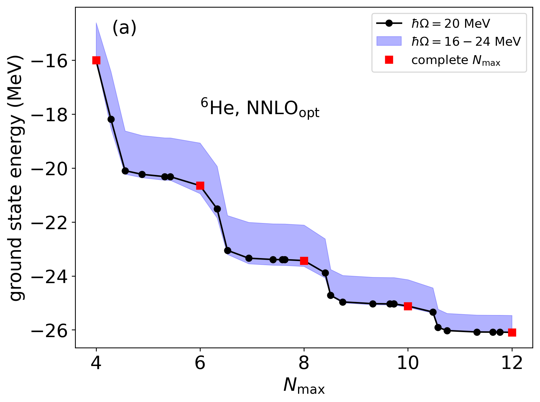
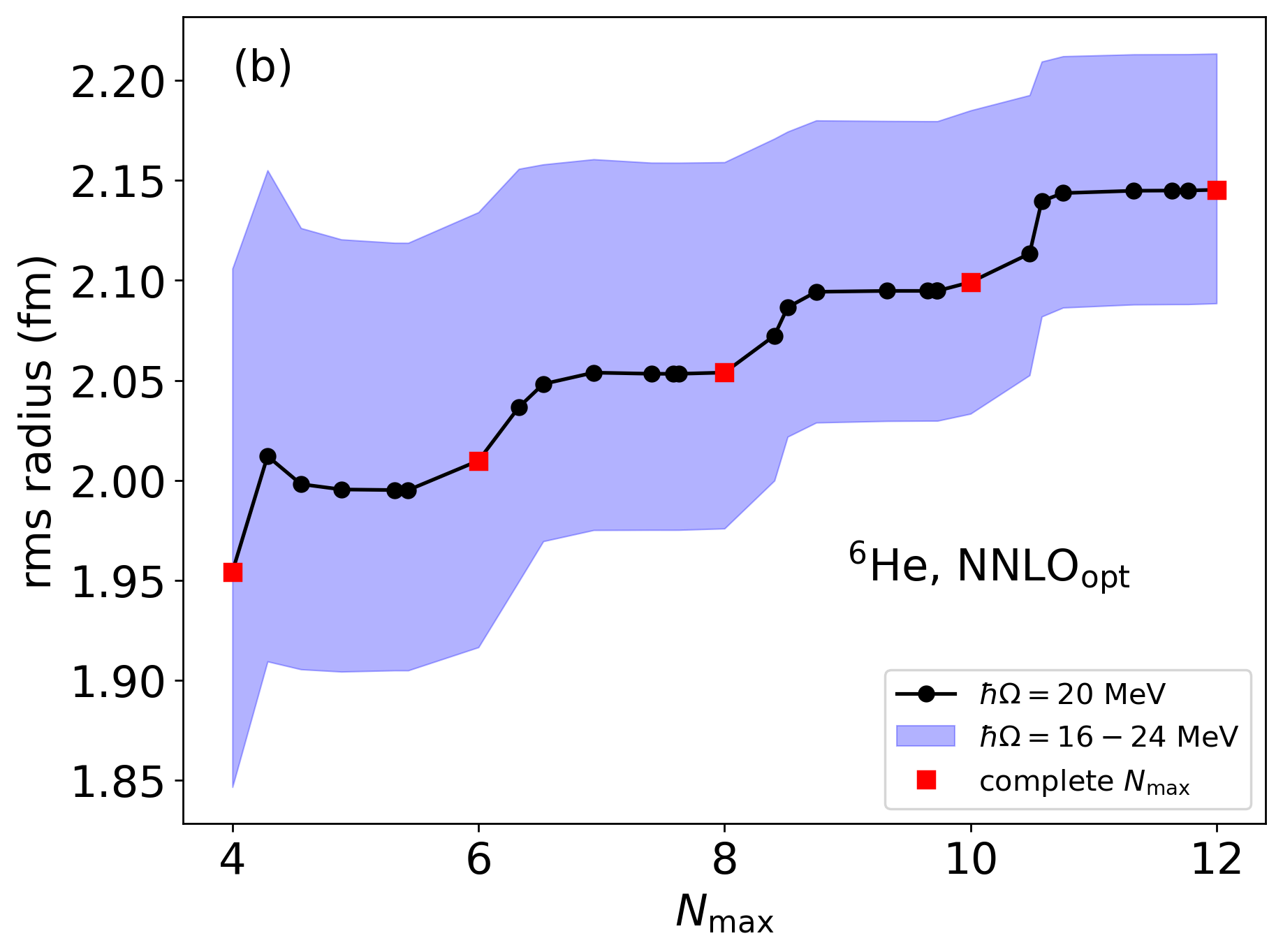
Using these SA model spaces in a structure calculation, the value of the corresponding structure observables is shown in Fig. 1, with Fig. 1(a) showing the ground state energy, and Fig. 1(b) showing the root-mean-square (rms) matter radius. The red squares correspond to calculations in the complete model spaces, while the black dots correspond to symmetry-adapted model spaces at different values. The black dots are placed along the -axis such that they indicate the percent of the model space included, e.g., a black dot near corresponds to a model space with a dimension roughly the size of the complete model space. Note that the bands indicate the variation in the results at nearby values. The line for the center value was selected according to , which typically yields the fastest convergence of rms radii. For 6He, this corresponds to MeV, which also emerges as the variational minimum in the ground state energy as increases [Fig. 1(a)].
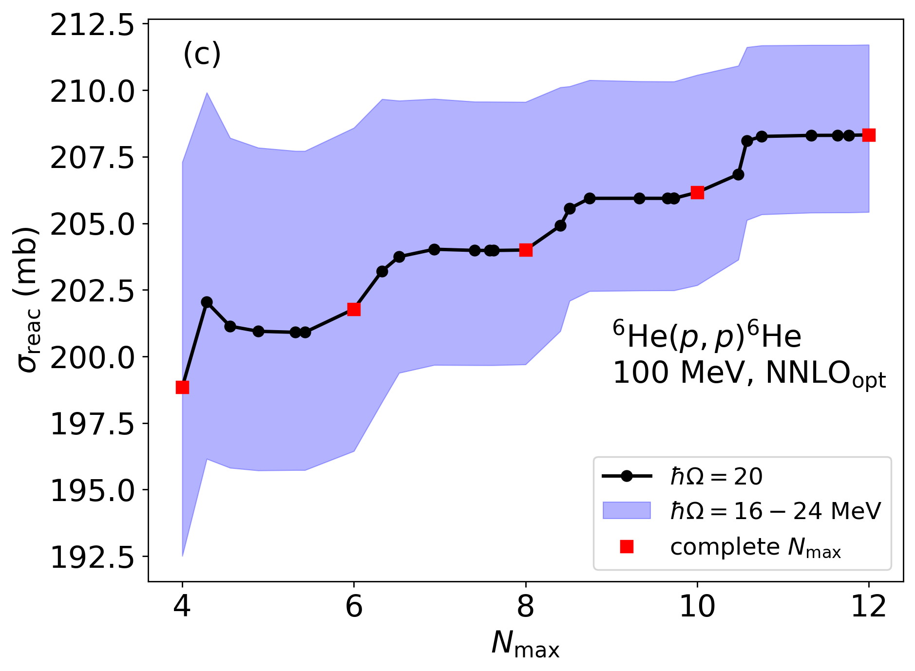
As shown by the structure observables in Fig. 1(a) and Fig. 1(b), in most cases, only a third of the model space (-, constructed from ) is already sufficient to reproduce the results of the complete model space. This is particularly true at the larger values. Notably, this pattern continues when examining scalar reaction observables. Namely, the reaction cross section for proton scattering at 100 MeV laboratory energy, , shown in Fig. 1(c), has a convergence pattern almost identical to that of the rms radius. From each of these results, it is worth noting that the variation in each observable with respect to is larger than the variation with respect to the model space selection – that is, the width of the bands is larger than the difference between neighboring black points in Fig. 1.
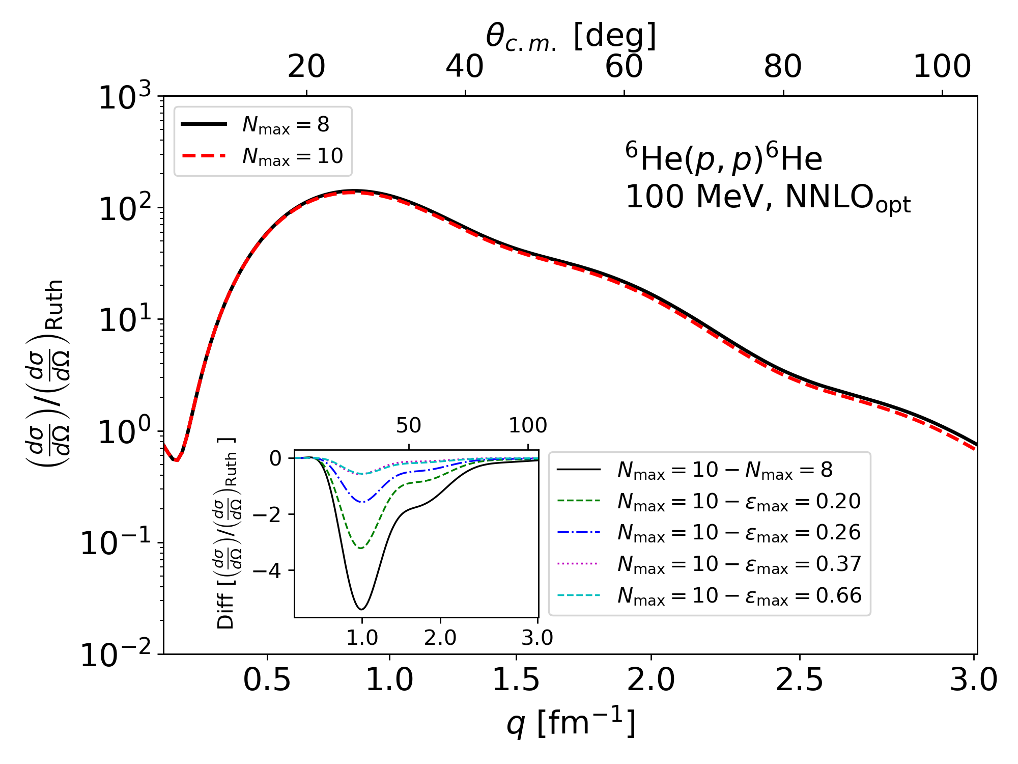
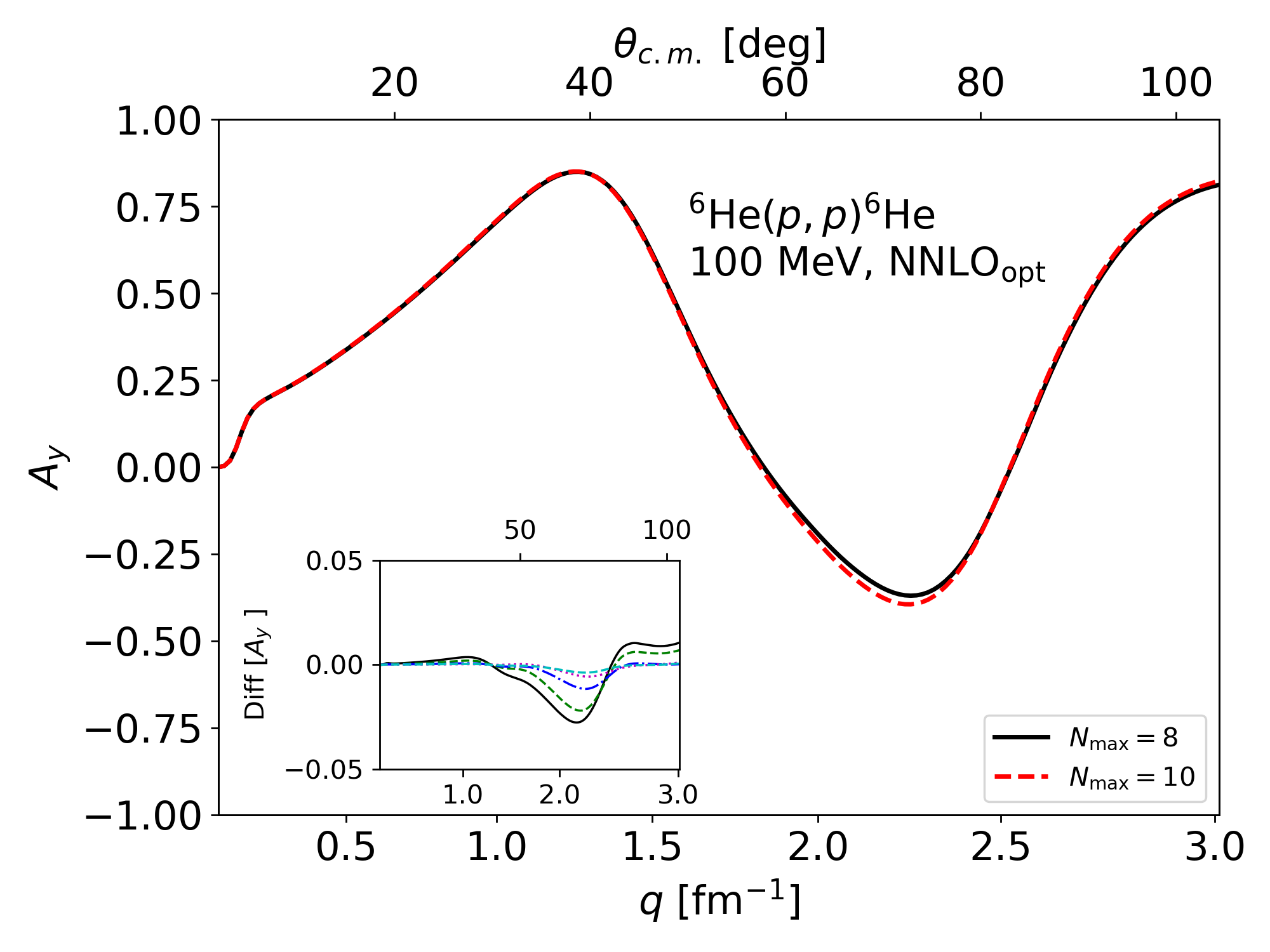
With an understanding of how the scalar observables converge for different model space selections, we can also examine functional observables, as shown in Figs. 2 and 3, which shows the differential cross section and analyzing power for proton scattering on 6He at 100 MeV. Comparing the and results (Fig. 2), small differences can be seen at large momentum transfers , where previous work has already shown these observables are slower to converge with respect to Burrows et al. (2019). Focusing on these two results, the inset shows the differences, where the solid black line shows how the results change from to , and the other lines show the differences in the and a selection of the model spaces. Similar to the structure observables, by approximately (or , roughly of the model space), the differences for the scattering observables in the SA and complete spaces are quite small. While not shown here, the convergence pattern for the spin rotation function is the same as the analyzing power .
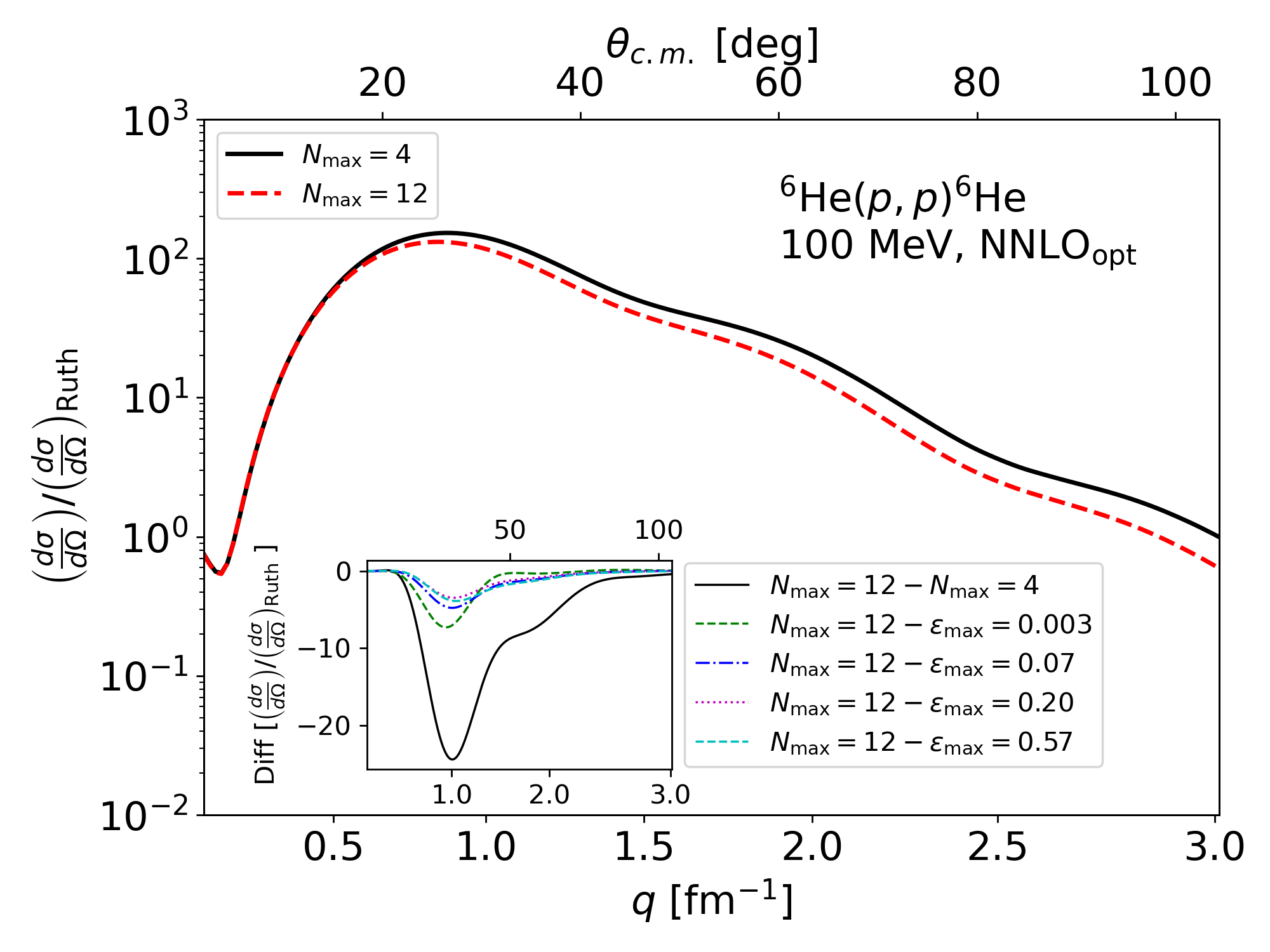
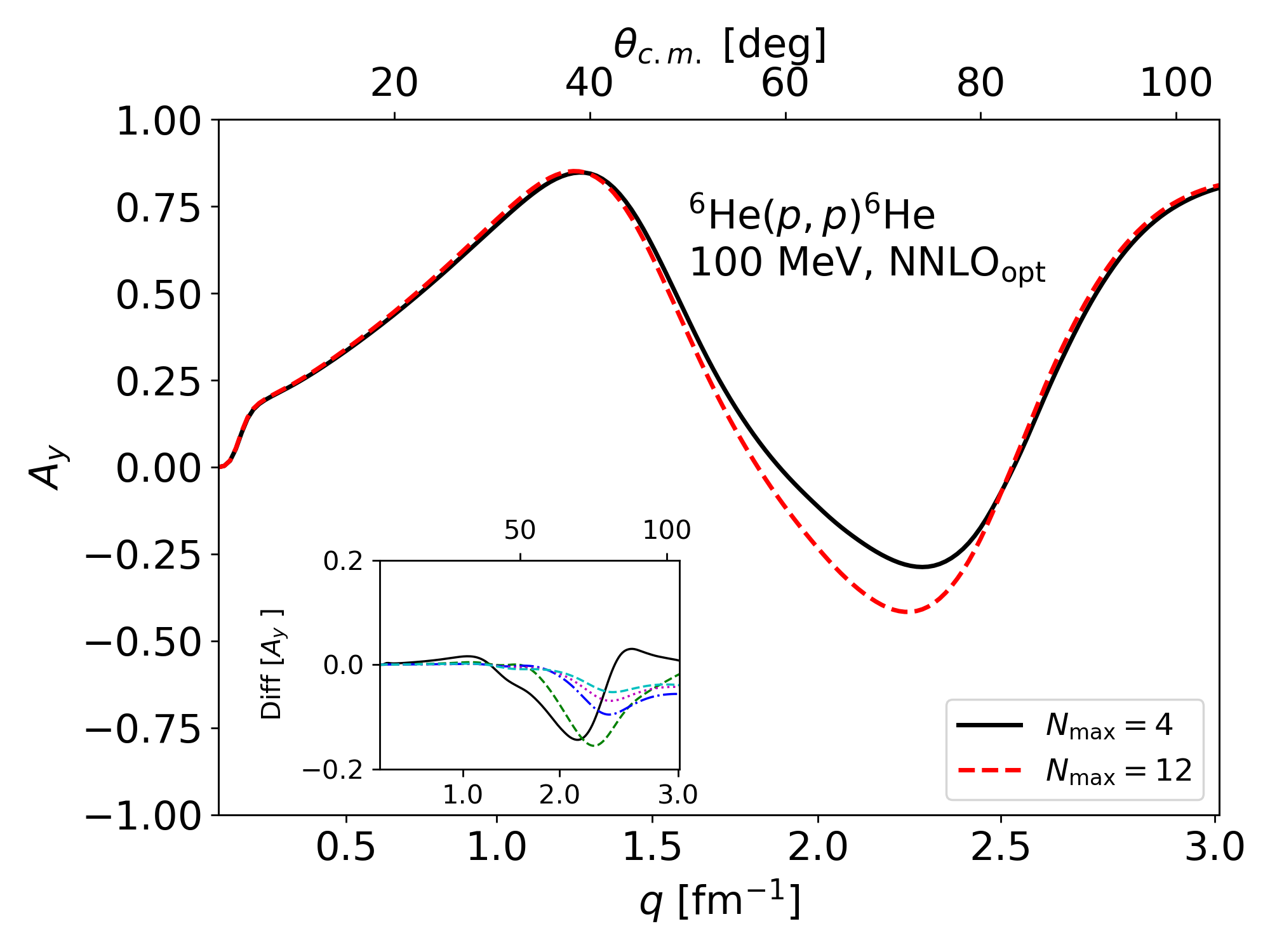
Similarly, Fig. 3 shows the same observables but compares against a broader span of , namely and . In this case, more significant differences are noticeable, as the results are much closer to convergence than . We see similar behavior as in the previous examples by applying the same process to construct SA model spaces. Namely, a well-constructed SA model space can reproduce the complete space results to within a few percent, which is typically smaller than the uncertainty from the variation or choice of the realistic interaction Burrows et al. (2019); Baker et al. (2023b).
III.2 Applying the selection procedure to proton scattering from 20Ne and 40Ca
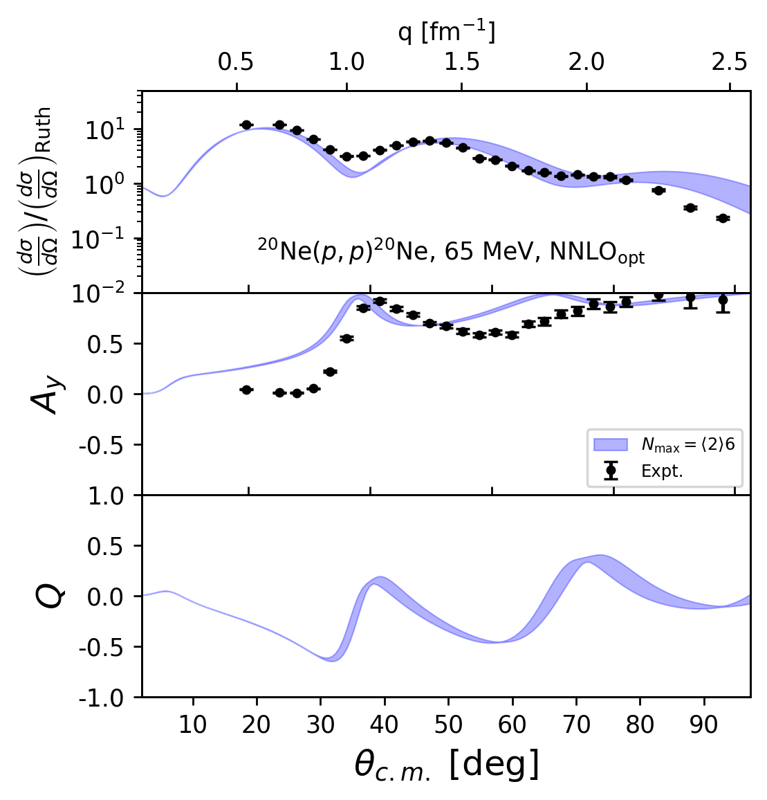
Acknowledging the convergence behavior of the observables for 6He as discussed in the previous section, we now turn to heavier nuclei, namely, the doubly open-shell nucleus 20Ne and the closed-shell 40Ca, where complete model spaces for sufficiently large are not feasible due to the rapid growth of the model space dimensions. Applying the same selection procedure for the ground state of 20Ne, we construct a model space and compute the nonlocal scalar densities and the spin-projected momentum distributions (where refers to the separate proton or neutron distributions) that enter the expression of Eq. (5) for the effective proton-nucleus interaction. Since experimental information for proton scattering from 20Ne in the energy regime above 60 MeV is limited, we show in Fig. 4 elastic scattering observables at 65 MeV calculated with three different values of the oscillator parameter indicated by the shaded band. The magnitude of the differential cross section (divided by the Rutherford cross section) is slightly underpredicted by the calculation, as is the first diffraction minimum. This small shift in the minimum corresponds to a slightly smaller rms matter radius from the theory calculation – here, fm – compared to the experimental value of fm Ozawa et al. (2001). This is consistent with the slightly smaller rms matter radii obtained by NNLOopt in light nuclei Burrows et al. (2019). Additionally, the calculation deviates from the data for momentum transfers larger than 2 fm-1. However, at the higher momentum transfers (or larger angles), the leading order in the spectator expansion should not be expected to be sufficient. Similarly, in addition to the slight radius discrepancy, rescattering terms may contribute to the first minimum in the differential cross section, as studies in few-body systems within the Faddeev framework Elster et al. (2008) suggest. The calculation of the analyzing power follows the general shape of the data but does not describe them well. This should also be taken as an indication that this energy is at the lower limit of applicability of the leading order term in the spectator expansion. The spin rotation function is shown as a prediction, as no experimental data exists.
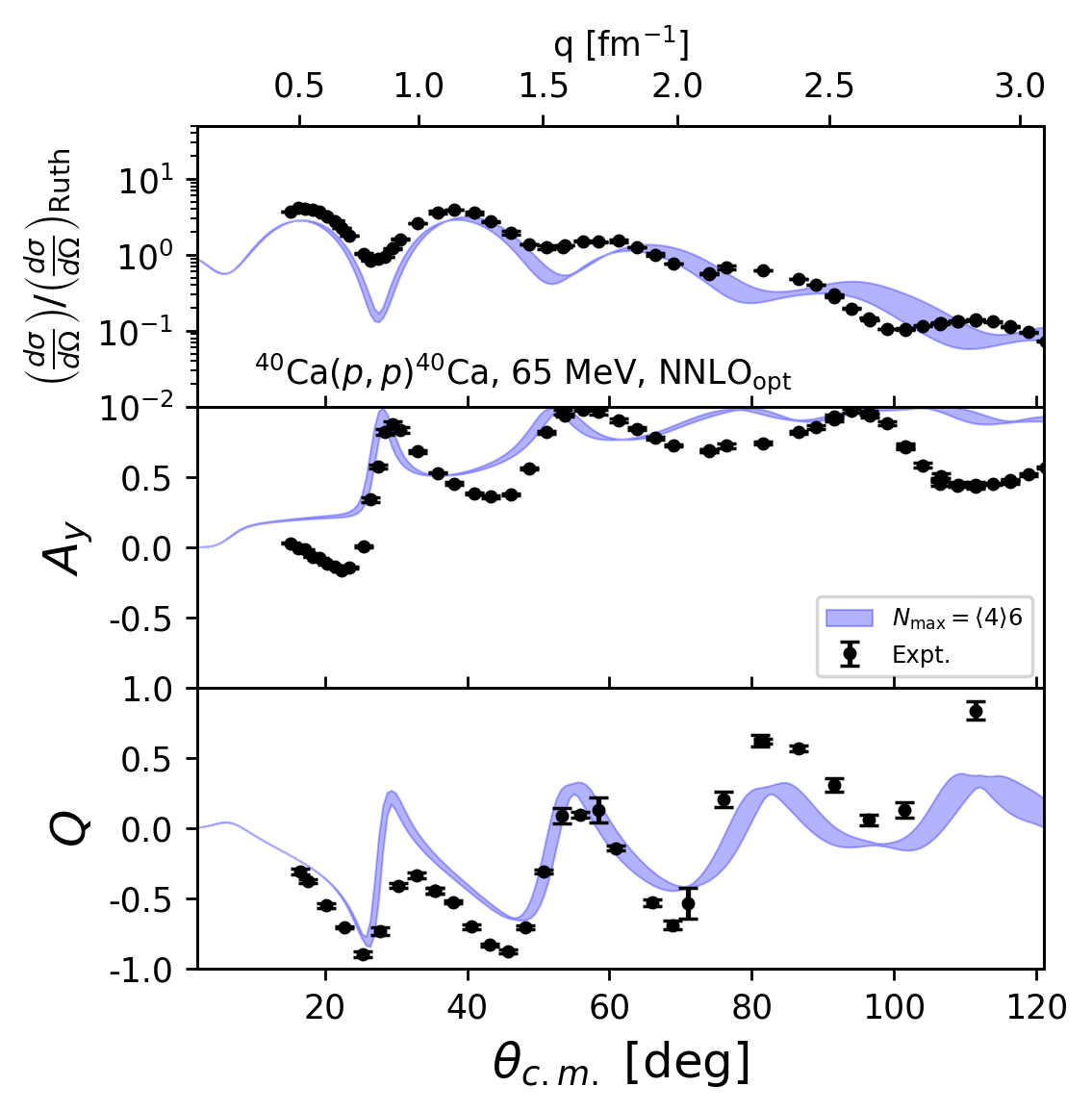
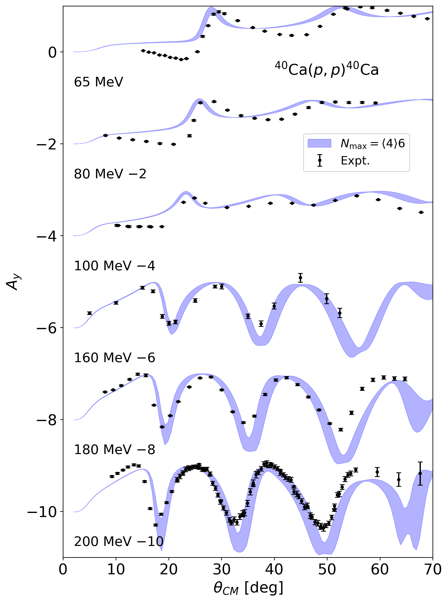
Turning to 40Ca, we employ the same procedure for computing the nonlocal scalar densities and the spin-projected momentum distributions. Unlike the dimensions of the 6He model spaces, the 40Ca model spaces grow significantly faster, with the complete space for having a dimension of 327,125,599. As a result, the important states provided by the same values () give smaller values (a model space fraction of only ) than for 6He. Elastic proton scattering from 40Ca is well measured in the energy regime between 65 and 200 projectile energy. Figure 5 shows the calculations for values between 11 and 13 MeV compared to the experimental data. Similar to the calculations for 20Ne, the differential cross section is slightly underpredicted for small momentum transfers, while the first diffraction minimum corresponds to the experimental one. Considering the diffraction pattern given by the first few minima, we see that it is wider than the experiment suggests. This may be related to the smaller calculated rms radius than the measured one. For the model spaces used here, this corresponds to an rms matter radius of fm, compared to the experimental charge radius of fm Angeli and Marinova (2013).
Comparing the differential cross section for 40Ca, Fig. 5, to the one for 20Ne at the same energy of 65 MeV, Fig. 4, we observe that the description of the Neon data at higher momentum transfer is better. This may be related to 20Ne being a deformed, doubly open-shell nucleus, sometimes considered to have an 16O core with two extra protons and neutrons in the outer shell (see, e.g., Ref. Dreyfuss et al. (2020) for the projection of the 20Ne ground state on the s-wave 16O, and Ref. Launey et al. (2021) for the cluster substructure revealed in the one-body density profile). If the nuclear density probed with proton scattering is less dense, rescattering, i.e., the next order in the multiple scattering expansion, may contribute less. Therefore, the leading order term gives a better description of the data. A similar effect has been seen in Ref. Burrows et al. (2020) in the very good description of the differential cross section for proton scattering from 6He and 8He.
At 65 MeV, the analyzing power and the spin rotation function are also measured for proton scattering from 40Ca. For small momentum transfers, is overpredicted by the calculation, while is more consistent with the data. As mentioned earlier, 65 MeV projectile energy is at the lower limit of the validity of the leading order in the spectator expansion, and corrections to the leading order should become visible. In Ref. Chinn et al. (1993), a modification of the many-body propagator due to the nuclear medium was introduced in a mean-field framework. In this work, calculations of the same observables for 40Ca show that those modifications improve the description of the spin-observables at 65 MeV while having no effect at higher energies.
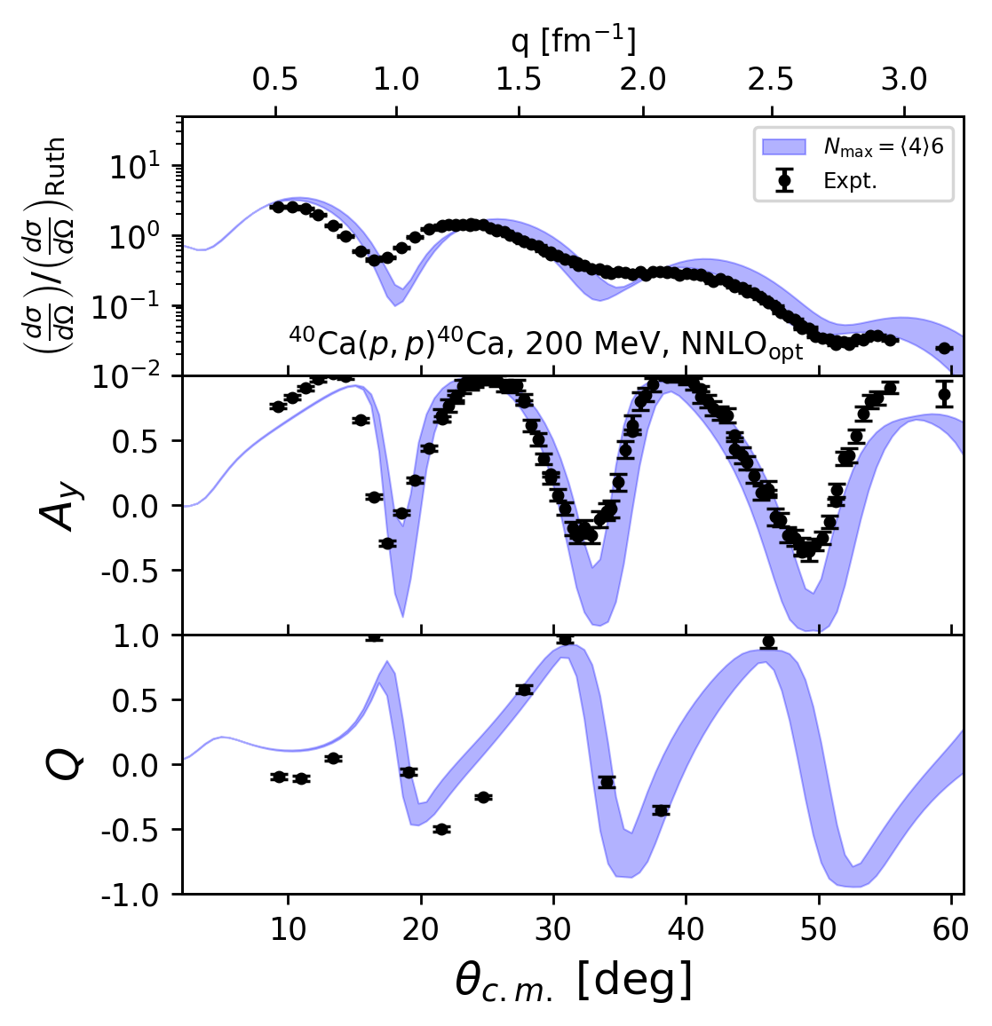
In Fig. 6, the observables for elastic proton scattering from 40Ca for 200 MeV projectile energy are shown for the same variation of and the same model space. Here, the pattern of both spin observables is very well described. The differential cross section is slightly overpredicted for small momentum transfers, and the first calculated diffraction minimum is shifted toward higher momentum transfers. Only the next minima line up better with the experiment. This slight shift of the first minimum is also seen in and .
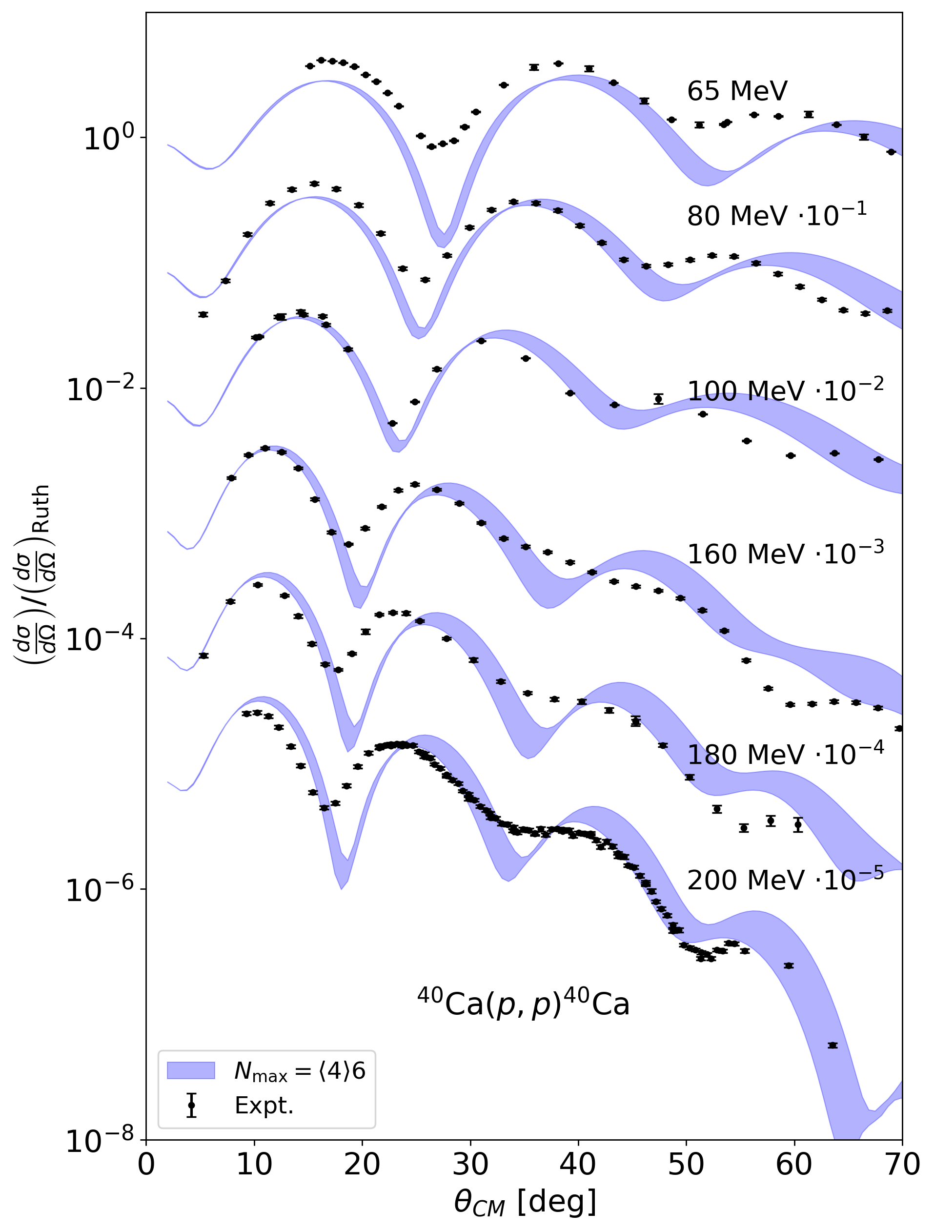
To study the energy dependence of elastic scattering observables, we show in Fig. 7 the differential cross section divided by the Rutherford cross section between 65 and 200 MeV projectile energy. The bands indicate the variation in for the many-body structure calculations. The dependence on observed for large angles suggests that larger model spaces may be needed to describe the data in this region. It is interesting to observe that for MeV, the overall agreement for fm-1 is remarkable, whereas the deviations at other energies may stem from rescattering effects not included at leading order (at lower energies) and properties of the interaction (at higher energies). Indeed, for the energies lower than 100 MeV, the differential cross section for small momentum transfers is slightly underpredicted, while for energies higher than 180 MeV, the experiment is overpredicted. In addition, while for the lower energies, the location of the first minimum corresponds exactly to the experimentally observed one, at energies higher than 100 MeV, the calculated first minimum shifts towards larger angles. This shift of the first diffraction minimum towards higher angles as a function of projectile energy was also observed in Ref. Vorabbi et al. (2024). Though in Born approximation and treating the nucleus as a black disk, the first minimum is directly related to the radius of the nucleus, the full calculation reveals an energy dependence of the location of the first minimum. Considering that the leading order term in the spectator expansion dominates the elastic scattering at higher energies, the predicted first minimum at 200 MeV being shifted to slightly larger angles is most likely related to the NNLOopt properties that are responsible for underpredicting the rms radius.
For a careful study of the energy dependence of the elastic scattering observables, we show in Fig. 8 the analyzing powers at the same energies given in Fig. 7. Here, we observe that the calculations match the minima and maxima of the experimental data well in the entire energy range shown in the figure. However, for the energies from 100 MeV and below, the experiment shows almost no analyzing power for small angles (momentum transfers), a feature that is not captured by the calculations, while above 100 MeV, the calculations describe the experiment very well. Similar to the differential cross section, the agreement of the analyzing power with the experiment is almost perfect at MeV.
IV Conclusions and Outlook
In this work, we concentrate on pursuing the theoretical description of the leading order term of the spectator expansion of the multiple scattering theory that employs SA-NCSM structure calculations and the first explorations of the SA-NCSM model space selection for scattering observables. This allows the consideration of heavier nuclei. In this selection procedure, all basis states are kept up to a given , while for higher , the model space is up-selected systematically using symmetry considerations. This procedure was successfully applied in considering structure phenomena across intermediate- and medium-mass nuclei and is now applied in the context of the construction of ab initio leading order effective interactions for elastic scattering. This effective interaction treats the interaction in the reaction part of the calculation on the same footing as in the structure part. This means that the leading order of the spectator expansion does not only take into account the spin of the projectile nucleon but also that of the struck target nucleon Burrows et al. (2020). Since this work concentrates on advancing the theoretical description towards heavier nuclei, we only use a single chiral potential, namely, NNLOopt Ekström et al. (2013).
Since our work is the first application of the selection procedure in the SA-NCSM calculations to scattering, we first thoroughly test it by calculating scattering observables for 6He. We chose this nucleus because scattering calculations using NCSM results with large model spaces have previously been studied Burrows et al. (2020). In addition, 6He is a light nucleus, but not closed-shell as 4He. After establishing the selection procedure, we calculate elastic proton scattering observables for 20Ne and, more importantly, 40Ca. For 40Ca we study observables in the energy range from 65 to 200 MeV. Our calculations for differential cross sections and spin observables compare favorably to the experiment. This paves the way for applying the SA-NCSM together with a selection procedure that only includes the nonnegligible configurations from the larger model spaces to calculations of the leading order effective interaction for nuclei with masses around -.
Acknowledgements.
This work was partly performed under the auspices of the U. S. Department of Energy under contract Nos. DE-FG02-93ER40756 and DE-SC0023532, and by the Czech Science Foundation (22-14497S). We thank Daniel Langr for his invaluable contributions to code development. The numerical computations benefited from computing resources provided by the Louisiana Optical Network Initiative and HPC resources provided by LSU, together with resources of the National Energy Research Scientific Computing Center, a U. S. DOE Office of Science User Facility located at Lawrence Berkeley National Laboratory, operated under contract No. DE-AC02-05CH11231.References
- Johnson et al. (2020) C. W. Johnson et al., J. Phys. G 47, 123001 (2020), arXiv:1912.00451 [nucl-th] .
- Rotureau et al. (2017) J. Rotureau, P. Danielewicz, G. Hagen, F. M. Nunes, and T. Papenbrock, Phys. Rev. C 95, 024315 (2017), arXiv:1611.04554 [nucl-th] .
- Idini et al. (2018) A. Idini, C. Barbieri, and P. Navrátil, J. Phys. Conf. Ser. 981, 012005 (2018).
- Burrows et al. (2024) M. Burrows, K. D. Launey, A. Mercenne, R. B. Baker, G. H. Sargsyan, T. Dytrych, and D. Langr, Phys. Rev. C 109, 014616 (2024), arXiv:2307.00202 [nucl-th] .
- Burrows et al. (2020) M. Burrows, R. B. Baker, Ch. Elster, S. P. Weppner, K. D. Launey, P. Maris, and G. Popa, Phys. Rev. C 102, 034606 (2020), arXiv:2005.00111 [nucl-th] .
- Gennari et al. (2018) M. Gennari, M. Vorabbi, A. Calci, and P. Navratil, Phys. Rev. C 97, 034619 (2018), arXiv:1712.02879 [nucl-th] .
- Arellano and Blanchon (2022) H. F. Arellano and G. Blanchon, Eur. Phys. J. A 58, 119 (2022), arXiv:2206.09461 [nucl-th] .
- Launey et al. (2016) K. D. Launey, T. Dytrych, and J. P. Draayer, Prog. Part. Nucl. Phys. 89, 101 (2016).
- Dytrych et al. (2020a) T. Dytrych, K. D. Launey, J. P. Draayer, D. J. Rowe, J. L. Wood, G. Rosensteel, C. Bahri, D. Langr, and R. B. Baker, Phys. Rev. Lett. 124, 042501 (2020a), arXiv:1810.05757 [nucl-th] .
- Launey et al. (2021) K. D. Launey, A. Mercenne, and T. Dytrych, Annu. Rev. Nucl. Part. Sci. 71, 253 (2021).
- Burrows et al. (2019) M. Burrows, Ch. Elster, S. P. Weppner, K. D. Launey, P. Maris, A. Nogga, and G. Popa, Phys. Rev. C 99, 044603 (2019), arXiv:1810.06442 [nucl-th] .
- Baker et al. (2023a) R. B. Baker, M. Burrows, C. Elster, K. D. Launey, P. Maris, G. Popa, and S. P. Weppner, Front. Phys. 10, 1071971 (2023a), arXiv:2301.04293 [nucl-th] .
- Burrows et al. (2023) M. Burrows, R. B. Baker, S. Bacca, K. D. Launey, T. Dytrych, and D. Langr, (2023), arXiv:2312.09782 [nucl-th] .
- Ekström et al. (2013) A. Ekström, G. Baardsen, C. Forssén, G. Hagen, M. Hjorth-Jensen, G. R. Jansen, R. Machleidt, W. Nazarewicz, et al., Phys. Rev. Lett. 110, 192502 (2013).
- Henderson et al. (2018) J. Henderson et al., Phys. Lett. B 782, 468 (2018), arXiv:1709.03948 [nucl-ex] .
- Ruotsalainen et al. (2019) P. Ruotsalainen, J. Henderson, G. Hackman, G. H. Sargsyan, K. D. Launey, A. Saxena, P. C. Srivastava, S. R. Stroberg, T. Grahn, J. Pakarinen, G. C. Ball, R. Julin, P. T. Greenlees, J. Smallcombe, C. Andreoiu, N. Bernier, M. Bowry, M. Buckner, R. Caballero-Folch, A. Chester, S. Cruz, L. J. Evitts, R. Frederick, A. B. Garnsworthy, M. Holl, A. Kurkjian, D. Kisliuk, K. G. Leach, E. McGee, J. Measures, D. Mücher, J. Park, F. Sarazin, J. K. Smith, D. Southall, K. Starosta, C. E. Svensson, K. Whitmore, M. Williams, and C. Y. Wu, Phys. Rev. C 99, 051301 (2019).
- Launey et al. (2018) K. D. Launey, A. Mercenne, G. H. Sargsyan, H. Shows, R. B. Baker, M. E. Miora, T. Dytrych, and J. P. Draayer, in Proceedings of the 4th International Workshop on “State of the Art in Nuclear Cluster Physics” (SOTANCP4), Texas (AIP Conf. Proc., 2018).
- Miller et al. (2022) S. B. S. Miller, A. Ekström, and K. Hebeler, Phys. Rev. C 106, 024001 (2022).
- Baker et al. (2020) R. B. Baker, K. D. Launey, S. Bacca, N. N. Dinur, and T. Dytrych, Phys. Rev. C 102, 014320 (2020).
- Sargsyan et al. (2022) G. H. Sargsyan, K. D. Launey, M. T. Burkey, A. T. Gallant, N. D. Scielzo, G. Savard, A. Mercenne, T. Dytrych, D. Langr, L. Varriano, B. Longfellow, T. Hirsh, and J. P. Draayer, Phys. Rev. Lett. 128, 202503 (2022), arXiv:2107.10389 [nucl-th] .
- Vorabbi et al. (2024) M. Vorabbi, C. Barbieri, V. Somà, P. Finelli, and C. Giusti, Phys. Rev. C 109, 034613 (2024), arXiv:2309.04226 [nucl-th] .
- Dytrych et al. (2020b) T. Dytrych, K. D. Launey, J. P. Draayer, D. J. Rowe, J. L. Wood, G. Rosensteel, C. Bahri, D. Langr, and R. B. Baker, Phys. Rev. Lett. 124, 042501 (2020b).
- Akiyama and Draayer (1973) Y. Akiyama and J. P. Draayer, Comput. Phys. Commun. 5, 405 (1973).
- Draayer et al. (1989) J. P. Draayer, Y. Leschber, S. C. Park, and R. Lopez, Comput. Phys. Commun. 56, 279 (1989).
- Langr et al. (2019) D. Langr, T. Dytrych, K. D. Launey, and J. P. Draayer, The International Journal of High Performance Computing Applications 33, 522 (2019).
- Oberhuber et al. (2021) T. Oberhuber, T. Dytrych, K. D. Launey, D. Langr, and J. P. Draayer, Discrete & Continuous Dynamical Systems-S 14, 1111 (2021).
- Launey et al. (2020) K. D. Launey, T. Dytrych, G. H. Sargsyan, R. B. Baker, and J. P. Draayer, Eur. Phys. J. Spec. Top. 229, 2429 (2020).
- Heller et al. (2023) N. D. Heller, G. H. Sargsyan, K. D. Launey, C. W. Johnson, T. Dytrych, and J. P. Draayer, Phys. Rev. C 108, 024304 (2023), arXiv:2205.06943 [nucl-th] .
- Verhaar (1960) B. J. Verhaar, Nucl. Phys. 21, 508 (1960).
- Hecht (1971) K. T. Hecht, Nucl. Phys. A 170, 34 (1971).
- Siciliano and Thaler (1977) E. R. Siciliano and R. M. Thaler, Phys. Rev. C16, 1322 (1977).
- Burrows et al. (2018) M. Burrows, C. Elster, G. Popa, K. D. Launey, A. Nogga, and P. Maris, Phys. Rev. C 97, 024325 (2018), arXiv:1711.07080 [nucl-th] .
- Wolfenstein and Ashkin (1952) L. Wolfenstein and J. Ashkin, Phys. Rev. 85, 947 (1952).
- Wolfenstein (1956) L. Wolfenstein, Ann. Rev. Nucl. Part. Sci. 6, 43 (1956).
- Møller (1945) C. Møller, K. Dan. Vidensk. Sels. Mat. Fys. Medd. 23, 1 (1945).
- Rodberg and Thaler (1967) L. Rodberg and R. Thaler, Introduction of the Quantum Theory of Scattering, Pure and Applied Physics, Vol 26 (Academic Press, 1967).
- Baker et al. (2023b) R. B. Baker, M. Burrows, C. Elster, P. Maris, G. Popa, and S. P. Weppner, Phys. Rev. C 108, 044617 (2023b), arXiv:2306.12597 [nucl-th] .
- Ozawa et al. (2001) A. Ozawa, T. Suzuki, and I. Tanihata, Nuclear Physics A 693, 32 (2001), radioactive Nuclear Beams.
- Elster et al. (2008) C. Elster, T. Lin, W. Glockle, and S. Jeschonnek, Phys. Rev. C 78, 034002 (2008).
- Angeli and Marinova (2013) I. Angeli and K. Marinova, Atomic Data and Nuclear Data Tables 99, 69 (2013).
- Dreyfuss et al. (2020) A. C. Dreyfuss, K. D. Launey, J. E. Escher, G. H. Sargsyan, R. B. Baker, T. Dytrych, and J. P. Draayer, Phys. Rev. C 102, 044608 (2020).
- Chinn et al. (1993) C. R. Chinn, Ch. Elster, and R. M. Thaler, Phys. Rev. C 48, 2956 (1993).
- Sakaguchi et al. (1979) H. Sakaguchi, M. Nakamura, K. Hatanaka, A. Goto, T. Noro, F. Ohtani, H. Sakamoto, and S. Kobayashi, Phys. Lett. B 89, 40 (1979).
- Sakaguchi et al. (1986) H. Sakaguchi, M. Yosoi, M. Nakamura, T. Noro, H. Sakamoto, T. Ichihara, M. Ieiri, Y. Takeuchi, H. Togawa, T. T., H. Ikegami, and S. Kobayashi, J. Phys. Soc. Japan Suppl. 55, 61 (1986).
- Stephenson (1985a) E. J. Stephenson, in Antinucleon and Nucleon-Nucleon Interactions, edited by G. Walker et al. (Plenum Press, NY, 1985) p. 299, Telluride Co.
- Seifert et al. (1993) H. Seifert et al., Phys. Rev. C 47, 1615 (1993).
- Stephenson (1985b) E. Stephenson, J. Phys.Soc. Jpn (Suppl.) 55, 316 (1985b).
- Nadasen et al. (1981) A. Nadasen, P. Schwandt, P. P. Singh, W. W. Jacobs, A. D. Bacher, P. T. Debevec, M. D. Kaitchuck, and J. T. Meek, Phys. Rev. C 23, 1023 (1981).
- H.Seifert (1990) H.Seifert, Ph.D. thesis, University of Maryland (1990).
- van Oers (1971) W. T. H. van Oers, Phys. Rev. C 3, 1550 (1971).
- Schwandt et al. (1982) P. Schwandt, H. O. Meyer, W. W. Jacobs, A. D. Bacher, S. E. Vigdor, M. D. Kaitchuck, and T. R. Donoghue, Phys. Rev. C 26, 55 (1982).
| dimension | |||
| threshold | |||
| 4 | - | 905 | 1 |
| 6 | 1,121 | 0.14 | |
| 2,189 | 0.28 | ||
| 3,477 | 0.44 | ||
| 5,182 | 0.66 | ||
| 5,611 | 0.71 | ||
| 6 | - | 7,854 | 1 |
| 8 | 8,083 | 0.16 | |
| 12,972 | 0.26 | ||
| 23,064 | 0.47 | ||
| 34,624 | 0.70 | ||
| 38,969 | 0.79 | ||
| 40,131 | 0.81 | ||
| 8 | - | 49,248 | 1 |
| 10 | 49,742 | 0.20 | |
| 62,898 | 0.26 | ||
| 91,417 | 0.37 | ||
| 162,196 | 0.66 | ||
| 202,435 | 0.83 | ||
| 211,522 | 0.86 | ||
| 212,039 | 0.87 | ||
| 10 | - | 245,082 | 1 |
| 12 | 246,043 | 0.24 | |
| 296,552 | 0.29 | ||
| 385,576 | 0.38 | ||
| 680,062 | 0.66 | ||
| 837,611 | 0.82 | ||
| 905,918 | 0.88 | ||
| 12 | - | 1,024,654 | 1 |
 |
 |
 |
 |
 |
 |
 |