Multi-Robot Planning for Filming Groups of Moving Actors Leveraging Submodularity and Pixel Density

Abstract

Observing and filming a group of moving actors with a team of aerial robots is a challenging problem that combines elements of multi-robot coordination, coverage, and view planning. A single camera may observe multiple actors at once, and the robot team may observe individual actors from multiple views. As actors move about, groups may split, merge, and reform, and robots filming these actors should be able to adapt smoothly to such changes in actor formations. Rather than adopt an approach based on explicit formations or assignments, we propose an approach based on optimizing views directly. We model actors as moving polyhedra and compute approximate pixel densities for each face and camera view. Then, we propose an objective that exhibits diminishing returns as pixel densities increase from repeated observation. This gives rise to a multi-robot perception planning problem which we solve via a combination of value iteration and greedy submodular maximization. We evaluate our approach on challenging scenarios modeled after various kinds of social behaviors and featuring different numbers of robots and actors and observe that robot assignments and formations arise implicitly based on the movements of groups of actors. Simulation results demonstrate that our approach consistently outperforms baselines, and in addition to performing well with the planner’s approximation of pixel densities our approach also performs comparably for evaluation based on rendered views. Overall, the multi-round variant of the sequential planner we propose meets (within 1%) or exceeds the formation and assignment baselines in all scenarios we consider.

Figure 1: A team of robots work together to film an unstructured scene with multiple moving actors splitting and merging.

I Introduction

Uncrewed aerial vehicles (UAVs) are widely applicable as mobile sensing and camera platforms. UAVs provide the ability to position a camera anywhere in 3D space, opening up the door to many possibilities across cinematography, inspection, and search and rescue. Because of this, UAVs are uniquely suited to capture unscripted scenarios such as team sports or animal behaviors. Additionally, when operating in a team, UAVs are able to capture multiple viewpoints simultaneously which can enable filming [1] or reconstructing [2, 3, 4] one or more people from multiple perspectives. Filming an unstructured group of actors introduces additional complexity—groups may split, spread out, and reform in various ways. This complexity can be ameliorated when this group motion is structured. Groups that move as a unit could be abstracted as a single actor and filmed by a team of UAVs flying in formation [2, 3]. Alternatively, an assignment scheme [5] could match UAVs to individual actors or groups that move together. Yet, groups of people in relevant settings—such as a team sport, a dance, a race—may frequently split, rejoin, and reorganize in ways that are prone to break formation and assignment schemes. This motivates development of systems that can optimize the robots’ collective views more directly.

I-A Related work

A large part of this work revolves around design of an objective for filming groups of moving actors with multiple robots. Mapping or exploring unknown environments is often closely tied to reconstruction (e.g. in the form of a mesh). These works differ from our approach in that they typically represent the environment with an occupancy grid, but objectives that capture observations of surfaces or that include terms based on distance or incidence angle have similar intent as what we propose [6, 7]. Papers that focus on reconstruction of known static or dynamic environments [8, 9, 10, 11] are also closely related to our approach. From the perspective of perceptual reward, Roberts et al. [10] propose a submodular objective based on covering hemispheres of viewing angles for each face with increasing hemispherical coverage given to closer views. An objective such as this could be applied to our setting by summing over time-steps and treating each instant like a static scene. The approach we propose does not directly reward different viewing angles of individual surface elements but instead seeks to maximize the collective density of pixels, following [11]. Additionally, like Roberts et al. [10], we propose a formulation based on a submodular objective. Our Square-Root-PPA objective is a submodular variation of the Pixel-Per-Area (PPA) objective by Jiang and Isler [11].

Given the design of the perception objective, the robots must plan to maximize that objective. Submodular optimization [12, 13] can solve many multi-robot perception, sensing and coverage problems with guarantees on suboptimality [14, 15, 16, 17]. Often, this takes the form of a guarantee that the worst case perception reward will be no worse than half of optimal [13]. Then, like Bucker et al. [1] we solve the single-robot sub-problems optimally with value iteration on a directed graph which is possible because view rewards for individual robots form a sum. Because rewards for individual robots are additive and not submodular, methods for single-robot informative (submodular) path planning are not relevant to this setting [18, 15, 19], and submodularity is only relevant to the multi-robot problem. Alternatively, other methods for solving multi-robot active perception problems such as Dec-MCTS [20] could be applicable. However, solving the single-robot perception planning problem by methods like Monte-Carlo tree search [20, 21, 22, 23] would not be necessary for the same reason as before.

Finally, the aforementioned methods optimize routes and views directly. These methods can provide flexibility in movement and capacity to cover different actors at different times. On the other hand, methods for filming and reconstruction based on formations [2, 3] or controllers centered on subjects being filmed [24] may not behave well if the people being filmed do not move as like one person.

I-B Contributions

In this work we introduce a method that pairs perception planning with a videography application to coordinate multiple UAVs to obtain diverse views of multiple moving actors. We present an objective that approximates pixel densities over the surfaces of the actors and exhibits diminishing returns with repeat observation. This extends the pixel-per-area (PPA) density approximation that Jiang and Isler [11] propose with a mechanism for obtaining diminishing returns (producing square-root-PPA or SRPPA). This in turn enables multi-robot application. Likewise, our choice of the SRPPA objective extends the planning approach by Bucker et al. [1] to the multi-actor by enabling reasoning about the quality of views of different actors. Moreover, our analysis proves that SRPPA is monotonic and submodular. This enables application of submodular maximization methods to jointly optimize views across the multi-robot team. The results compare submodular maximization methods to formation and assignment baselines in a variety of scenarios that simulate challenging behaviors (splitting, merging, reorganization) and higher level scenarios (social groups, races). Our approach meets (within 1%) or exceeds the performance of our baselines all scenarios. and behaves intuitively such as by implicitly producing formations or assignments.

Additionally, an extension of this work that introduces non-collision constraints between robots and an objective implementation based on rendered views is also under review [25]. While the key contribution by Suresh et al. [25] is application to a more realistic setting, this paper’s unique contribution includes general analysis of submodularity of SRPPA and similar objectives—this is non-trivial because SRPPA does not readily reduce to a form of coverage—and evaluation in an unconstrained setting where suboptimality guarantees hold strictly and with scenarios that emphasize the role of cooperative view planning.

II Background

In this work, we apply methods for submodular optimization to coordinate the multi-robot teams and to analysis our perception objective. To begin, consider a set $\Omega=\bigcup_{r\in 1:N}{\mathscr{U}}_{r}$ that might represent possible assignments of actions to robots where each ${\mathscr{U}}_{r}$ represents a (disjoint) local sets of actions associated with each robot $r\in{\mathcal{R}}=\{1,\ldots,{N^{\mathrm{r}}}\}$. The following subsections build tools that operate on these sets when solving planning problems.

II-A Submodularity and monotonicity

The objectives in the perception planning problems we study map sets of actions—we call them set functions—to real numbers $g:2^{\Omega}\rightarrow$, and we can interpret the value of a set function as a reward. We will be interested in maximizing set functions subject to certain conditions. Generally, we are interested in set functions that are normalized $g(\emptyset)=0$, monotonic $g(A)\geq g(B)$ for $B\subseteq A\subseteq\Omega$, and submodular $g(A\cup c)-g(A)\leq g(B\cup c)-g(B)$ where $c\in\Omega\setminus A$. Monotonicity generally expresses the notion that more observations produce more reward or equivalently that the discrete derivative is positive. Submodularity is a monotonicity condition on the second discrete derivative [26] and expresses the notion that marginal gains decrease in the presence of more prior observations. Additionally, we will take some liberties with notation such as to replace unions with commas or to implicitly wrap elements in sets and so we will abbreviate marginal gains as follows $g(c|A)=g(A,c)-g(A)=g(A\cup c)-g(A)$ which we read as “the marginal gain for $c$ given $A$.”

II-B Submodular optimization for multi-robot coordination

In the problems we study, valid plans for the multi-robot team consist of at most one action from each robot’s local set. That is $X\in{\mathscr{I}}=\{X\subseteq\Omega\mid 1\geq|X\cap{\mathscr{U}}_{r}|,\forall r\in{\mathcal{R}}\}$ which forms a simple partition matroid [27, Sec. 39.4]. Thus, we wish to solve optimization problems of the form

$$X^{{\mathrm{opt}}}\in\operatorname*{arg\,max}_{x\in{\mathscr{I}}}g^{\mathrm{obj}}(X)$$ (1)

where $g^{\mathrm{obj}}$ is normalized, monotonic, and submodular. Greedy algorithms can solve these problems with various guarantees of solutions within a fraction of optimal, and these methods have been applied frequently to solve in robotics related to perception, coverage, and search [15, 16, 14]

III Problem formulation

Consider a team of ${N^{\mathrm{r}}}=|{\mathcal{R}}|$ robots with states $x_{r,t}\in X_{r}$ for $r\in{\mathcal{R}}$, where $X_{r}$ is a subset of the special euclidean group $SE(2)$, and a set of actions $u_{r,t}\in U_{r,t}$, where $U_{r,t}$ is the finite space of actions available to robot $r$ at time $t\in\{1,\ldots,T\}={\mathcal{T}}$. The robots film the actors ${\mathcal{A}}=\{1,\ldots,{N^{\mathrm{a}}}\}$ which have states $y_{a,t}\in SE(3)$, and we refer to an actor’s trajectory as $Y_{a}=[y_{a,1},y_{1,T}]$. Problem: Given known (or scripted) actor motions, the task is to select robot trajectories to maximize the objective $g^{\mathrm{obj}}$ which primarily represents the quality of the robots’ views of the actors over the course of the time horizon.

III-A Motion model

State transitions are governed by the following motion model:

$$x_{r,t+1}=f(x_{r,t},u_{r,t})$$ (2)

where $f$ constrains motion to state transitions within distance $D$ of the current state, with one of eight possible camera orientations. Additionally, we will refer to the robots’ yaw angle as ${\theta}_{r,t}$. Robots are able to rotate clock-wise or counter-clock wise by a $\pi/4$ radians at each time-step. The space of control actions $U_{r,t}$ thus encodes a finite list of adjacent positions and orientations, and we will treat this set as time-varying only to account for in-valid transitions—in our case we require the robot to remain in-bounds on a grid.

III-B Actor motion and representation

The robots seek to collectively film the actors which follow known trajectories $Y_{a}$. The actors (such as people, animals, or cars) are represented by simple polyhedra, in our case, a capped rectangular prism. Each actor $a$ contains a set of faces $F_{a}\subseteq{\mathcal{F}}$ where ${\mathcal{F}}$ is the total set of faces in the scene. Faces are parameterized by the normal $\vec{\eta_{f}}$, the area $A_{f}$, the face center position $\vec{p_{f}}$, and the weight $w_{f}$. We define the position and orientation of the faces in $F_{a}$ relative to the actor position $\vec{c_{a,t}}$ and rotation $\theta_{a,t}\in[0,2\pi]$ (and the corresponding rotation matrix $R_{a,t}$). See Fig. 2. Actor trajectories are not constrained in position or orientation.

Figure 2: Scene representation. Actors are modeled as capped hexagonal prisms, and move on trajectories $Y_{a}$ in the plane. Robots move in a grid located at height $d_{h}$.

III-C Camera and sensor model

The robots are equipped with cameras with which they observe and film the actors. For the purpose of planning we adopt a simplified quasi-two-dimensional camera model. In this model, cameras face forward, and observe in the actor plane within a horizontal viewing angle ${\gamma}$ (field-of-view) regardless of distance. While we do not model the full camera view frustums or occlusions, we do account for $d_{h}$, the height of the robots above the actors in distance calculations between actor faces and robots. Additionally, we cull back-sides of faces by checking whether the face normal is facing away from the camera. Otherwise, we do not do any raytracing or account for occlusions between different actors. Later, we will model view quality based on an approximation of the size of the face projected into the image sensor as determined by the distance and a check regarding whether a given face is in view. We also compare this simple camera model against a more realistic one in the rendering based evaluations in Sec. VI-C2.

III-D Assumptions

For the purpose of this paper, we assume centralized computation though there are applicable distributed solvers for the submodular optimization problems we discuss [28]. Robot and actor positions and orientations are known, and we require some additional instrumentation (e.g. GPS [2, 29, 3]) to track position. Additionally, actor motions are known or scripted. Although there are scripted scenarios are relevant to this work, predictions for unscripted scenarios (e.g. filming team sports) may only be accurate over a short horizon (e.g. based on a velocity output from a Kalman filter [30]) or require learned predictions. Likewise, objective evaluation (Sec. III-E) in expectation would not compromise our analysis but could significantly increase computation time. Finally, we ignore collisions and occlusions; this work focuses on the design of the SRPPA objective and behavior of the submodular optimization problem. Collision and occlusion-aware planning is the focus of our succeeding work [25].

III-E Objective function

The design of the perception objective $g^{\mathrm{obj}}$ for the videography task captures the following intuition:

• Maximum actor size: Select camera views to maximize size of actors in the field of view

• Maximum actor coverage: Robots should collectively keep all actors in view at all times and with uniform coverage quality

• View diversity: Prefer views that cover different sides of an actor versus many views of the same side

• Actor centering: Prefer centering actors in field of view

Following the description of the submodular maximization problem in Sec. II-B, we define the robots’ local action sets via tuples representing the assignment of a sequence of valid control actions ${\mathscr{U}}_{r}=\{(r,u_{r,1:T})\mid u_{r,t}\in U_{r,t}\}$ to robot $r\in{\mathcal{R}}$. Based on these sequences of control actions, we define the objective as a sum of path $g^{\mathrm{path}}$ and view $g^{\mathrm{view}}_{a,t}$ rewards over actors and time-steps

$$g^{\mathrm{obj}}(X) =g^{\mathrm{path}}(X)+\sum_{t=1}^{T}\sum_{f\in F_{a},\,a\in{\mathcal{A}}}g^{\mathrm{view}}_{f,t}(X)$$ (3)

for $X\in\Omega$ and given the predicted actor trajectories $Y_{a}$. We call this the Square-Root PPA (Pixels-Per-Area [11]) or SRPPA objective for reasons that will soon be clear. The path reward $g^{\mathrm{path}}(X)=\sum_{x\in X}w_{\mathrm{p}}(x)$ is a reward ($w_{\mathrm{p}}(x)\geq 0$) on the robots’ paths.

The function $g^{\mathrm{view}}$ represents the total view quality for a face at a given time. In order to satisfy suboptimality guarantees afforded by sequential greedy planning [12, 13] this view reward must be submodular and monotonic. The following expression applies a square-root in a way which will satisfy these requirements

$$g^{\mathrm{view}}_{f,t}(X)=w_{f}A_{f}\sqrt{g^{\mathrm{pixels}}_{f,t}(X)}$$ (4)

where $g^{\mathrm{pixels}}$ accumulates the sensing quality for a particular face $f$ of an actor across all robots and $w_{f}\geq 0$ is a designer weight which can prioritize actors (e.g. a speaker) or individual mesh faces (e.g. a person’s front or face).

The function $g^{\mathrm{pixels}}$ approximates the cumulative pixel density for a given face, and we will additionally weight this based on camera alignment. However, we must first define a few more terms. Defining the position of the robot as $\vec{p_{r}}$, the relative position of a particular face $f$ on actor $a$ is:

$$\vec{d_{r,f,t}}=(\vec{c_{a,t}}+R_{a,t}\vec{p_{f}})-\vec{p_{r}}.$$ (5)

Then, define the rotated face normal as $\vec{\eta}=R_{a,t}\vec{\eta_{f}}$. The weighted pixel density is as follows:

$$\begin{split}&g^{\mathrm{pixels}}_{f,t}(X)\\ &=\sum_{(r,u_{r,1:T})\in X}\alpha\text{INVIEW}_{f}(x_{r,t})\frac{(\vec{d_{r,f,t}}\cdot\vec{\eta})}{||d_{r,f,t}||^{3}}\frac{(\vec{d_{r,f,t}}\cdot\vec{\eta_{r}})}{||d_{r,f,t}||}\end{split}$$ (6)

where $||\cdot||$ is the 2-norm, INVIEW returns whether a given face is in the field of view and facing the robot and zero otherwise; $\vec{\eta_{r}}$ is a unit vector representing the robot heading; and $\alpha$ is the number of pixels per unit area at one meter. In this expression, the first ratio corresponds to computation of pixels-per-area and the second forms a weight that encourages robots to center faces in the camera view.

Remark 1 (Intuition for perception objective).

In (6), $g^{\mathrm{pixels}}$ approximates the cumulative density of pixels (weighted to encourage centering) for all robots observing each face. If we only maximized the sum of these terms, there would be no diminishing returns, and robots might just maximize reward for a single actor or face. The square-root in (4) introduces diminishing returns because growth of the square root slows as $g^{\mathrm{pixels}}$ increases (analysis in Sec. V states this formally). Generally, this encourages robots to cover actors uniformly at a moderate level versus individually at high levels.

IV Planning approach

In this work we seek to maximize $g^{\mathrm{obj}}$ (3) by optimizing robot trajectories given a set of actor trajectories. To simplify the problem we define two distinct planning subproblems: a single-robot planning subproblem, and a coordination subproblem. In the single-robot planning step, we seek an optimal trajectory for a single robot given actor trajectories. In the coordination step, we maximize overall sensing quality across all robots by sequencing multiple single-robot planning steps. Our planning approach is similar to that of Bucker et al. [1].

IV-A Single robot planning

We apply backward value iteration [31, Sec. 2.3.1.1] to solve the single robot planning problem optimally similarly as other works involving perception planning [2, 1, 16]. Backward value iteration operates by taking a single pass over $X_{r}\times{\mathcal{T}}$ going backward in time. For every state time pair, backward value iteration iterates over control actions and selects the one that maximizes the immediate reward plus the reward from the next state (which has already been visited) to the end of the horizon. This maximizes the perception objective $g^{\mathrm{obj}}$ for a single robot, possibly given other robots (fixed) decisions as well.

IV-B Sequential planning and coordination

We coordinate robots via sequential greedy planning. Through this process, robots each plan as described in Sec. IV-A and maximize $g^{\mathrm{obj}}$ conditional on the prior robots’ selections. Thus, the robots produce a greedy solution $X^{\mathrm{g}}=\{x_{1}^{\mathrm{g}},\ldots,x_{r}^{\mathrm{g}}\}$ by solving

$$x^{\mathrm{g}}_{r}\in\operatorname*{arg\,max}_{x\in{\mathscr{U}}_{r}}g^{\mathrm{obj}}(x|X_{1:r-1}^{\mathrm{g}})$$ (7)

in sequence via value iteration where $X_{1:r-1}^{\mathrm{g}}$ is the set of prior selections. Fisher et al. [13] proved the following suboptimality guarantee: if $g^{\mathrm{obj}}$ is monotonic, submodular, and normalized, then $g^{\mathrm{obj}}(X^{\mathrm{g}})\geq\frac{1}{2}g^{\mathrm{obj}}(X^{\mathrm{g}})$ given that $X^{\mathrm{opt}}$ is the optimal solution to (1).

IV-C Multiple rounds of greedy planning

Although a single pass of greedy planning guarantees solutions no worse than half of optimal, we are often able to improve these solutions in practice. We adopt a similar approach as McCammon et al. [32, Sec. 4.2] do for a surveying task. Specifically, robots replan by solving a slightly different single-robot subproblem

$$x^{\mathrm{mr}}_{r}\in\operatorname*{arg\,max}_{x\in{\mathscr{U}}_{r}}g^{\mathrm{obj}}(x|\hat{X}\setminus{\mathscr{U}}_{r})$$ (8)

where $\hat{X}\subseteq\Omega$ is the solution we wish to improve. Here, we modify (7) by removing any assignment to $r\in{\mathcal{R}}$ to allow that robot to replan. When planning in multiple rounds robots solve (8) in ${N^{\mathrm{mr}}}$ passes over ${\mathcal{R}}$. By this process, robots first produce a solution equivalent to $X^{\mathrm{g}}$ and in subsequent rounds may improve solution quality to produce $X^{\mathrm{mr}}$. Replanning by this process can never produce a worse solution, but there is no guarantee to for an improved or optimal solution either.

V Analysis

This section introduces the analysis of the monotonicity properties of the objective and applies that to guarantee bounded solution quality.

Theorem 1 (Monotonicity properties of SRPPA).

The SRPPA objective $g^{\mathrm{obj}}$ from (3) is normalized, monotonic, and submodular. Moreover, SRPPA satisfies alternating monotonicity conditions and is $n$-increasing for odd values of $n$ or else $n$-decreasing if even.

Corollary 1.1 (Bounded suboptimality).

Theorem 1 ensures that $g^{\mathrm{obj}}$ satisfies the requirements stated in Sec. IV-B for sequential (and multi-round) planning to produce solutions that satisfy $g^{\mathrm{obj}}(X^{\mathrm{g}})\geq\frac{1}{2}g^{\mathrm{obj}}(X^{\mathrm{g}})$. Additionally, $g^{\mathrm{obj}}$ is 3-increasing which is sufficient to guarantee bounded suboptimality in expectation for distributed optimization via the RSP algorithm [33, Theorem 9].

We include a full proof of Theorem 1 in Appendix A. The following lemma (which we prove in Appendix A-C) is key to our approach. We use this lemma to prove that $g^{\mathrm{view}}$ (4) transforms $g^{\mathrm{pixels}}$ (6) such that the resulting function is monotonic and submodular. The reader may refer to Appendix A-A or [26] for discussion of general monotonicity conditions.

Lemma 2 (Monotonicity for composing a real and a modular function).

Consider a monotonic, modular set function $g:\Omega\rightarrow_{\geq 0}$ and a real function $\psi:_{\geq 0}\rightarrow$. If $\psi$ is $m$-increasing (or decreasing) according to Def. 3, then their composition $\hat{g}(x)=\psi(g(x))$ is also $m$-increasing (or decreasing).

The rest of the proof of Theorem 1 is in Appendix A-D. The outline of this proof is as follows. First, we apply Lemma 2 to $g^{\mathrm{view}}$ and $g^{\mathrm{pixels}}$. Then, we apply results by Foldes and Hammer [26] to prove that the sum of terms in $g^{\mathrm{obj}}$ (3) preserves these monotonicity conditions. Finally, $g^{\mathrm{obj}}$ is normalized ($g^{\mathrm{obj}}(\emptyset)=0$) because all the terms are normalized.

Remark 2 (Transformations with other real functions).

Following Lemma 2, real functions other than the square root could be applied to implement diminishing returns. The functions $1-e^{-x}$ and $\log(x+1)$ are two other examples with alternating derivatives. Other functions such as variations of sigmoids $\frac{1}{1+e^{-x}}$ can produce monotonic submodular objectives that do not satisfy higher order monotonicity properties.

Additionally, $g^{\mathrm{obj}}$ may not initially appear to belong to any specific class of functions aside from satisfying a few monotonicity conditions, but there is some additional structure that we can point out.

Remark 3 (Relationship between coverage and alternating derivatives).

In addition to being monotonic and submodular, $g^{\mathrm{obj}}$ satisfies alternating monotonicity conditions because derivatives of the square root have alternating signs (Theorem 1). We have remarked before that this same alternating derivatives property applies to a form of weighted coverage objective [33, Theorem 9], and others have made similar observations [34, 35]. One may suspect that having alternating derivatives is sufficient for a set function to be a form of weighted coverage though we are not yet aware of a published proof of this statement..

VI Methods

This section introduces baseline planners we compare against and their implementations, evaluation scenarios, and approaches to evaluating perception performance.

VI-A Planner baselines

VI-A1 Myopic planner

Myopic planning refers to planning without coordination with the rest of the team. Specifically, robots run the single-robot planner (Sec. IV-A) for themselves only without sharing results like in the sequential planning scheme. In [36], we observe that robots tend to maximize view quality but may converge to the same views at the expense of the global view quality.

VI-A2 Formation planner

Formation planning is a simple and effective approach for filming groups of moving actors [2, 3]. For our baseline we implemented a formation planner that places robots evenly on a circle centered on the centroid of the actor positions with a radius based on the distance of the furthest actor from the center plus a safety margin. In essence, we assume the group of actors behaves behaves like a single “meta-actor.” To improve performance, each robot also focuses its view on the nearest actor. This approach would be effective in many real world scenarios but struggles as groups move apart or become less circular.

VI-A3 Assignment planner

With the assignment planner, each robot is tasked with observing only a subset of the actors. The assignment planner attempts to evenly distribute actors to robots and produces an assignment that is fixed for the entire planning horizon. If the number of actors is larger than the number of robots, the set of actors will be distributed equally among the robots, but some actors will not be assigned if the set is not evenly divisible. If the number of robots is larger than the number of actors, each robot will be assigned a single actor with some overlapping assignments.

VI-B Scenarios

We evaluate our planners and baselines against a set of hand-crafted scenarios (Fig. 3) designed to mimic challenging multi-robot filming situations and specify the number of robots and the actor trajectories. A subset of the scenarios were designed to act as canonical points of comparison, such as stationary targets in a tight cluster (Fig. 3(a)) or a group uniformly separating (Fig. 3(f)). In these cases, we expect similar performance between planners. Some scenarios are designed to target specific weaknesses of our baselines. In the cross-mix scenario, 6 actors start in pairs, then cross and mix together such that two of the three groups have swapped members; this can be challenging for planners that rely on fixed robot-actor pairings. The track-runners and priority-runners scenarios mimic real life situations relevant to sports cinematography where groups periodically spread and join or where one character i.e. the leader in a race, may be a more important subject for filming than others. The priority-speaker scenario mimics a gathering in which a group of moving actors is addressed by a stationary speaker. In each “priority” scenario, one actor is given a higher weight than the others. Broadly speaking, a desirable outcome is to focus more camera attention on prioritized actors while obtaining fewer or more distant views of the rest of the actors in the scene. Scenarios with a large degree of group splitting such as four-split, split-and-join, and spreadout-group pose a challenge for applying formation planning approaches [2] to multi-robot settings.

(a) Cluster; $N_{r}\!=\!4$, $N_{a}\!=\!6$

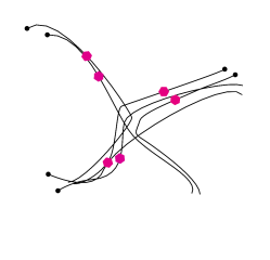
(b) Cross-Mix; $N_{r}\!=\!4$, $N_{a}\!=\!6$

(c) Four-Split; $N_{r}\!=\!4$, $N_{a}\!=\!4$

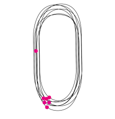
(d) Priority-Runners; $N_{r}\!=\!5$, $N_{a}\!=\!7$

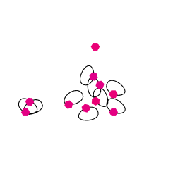
(e) Priority-Speaker; $N_{r}\!\!=\!\!5$, $N_{a}\!\!=\!10$

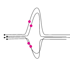
(f) Split-and-Join; $N_{r}\!=\!4$, $N_{a}\!=\!4$

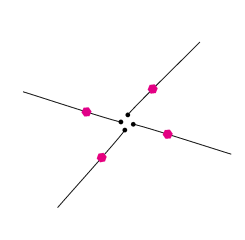
(g) Spreadout-Group; $N_{r}\!=\!4$, $N_{a}\!=\!4$

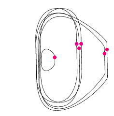
(h) Track-Runners; $N_{r}\!=\!5$, $N_{a}\!=\!6$

Figure 3: Summary of experiment scenarios. Each scenario is shown from a top down view, with each actor represented as a red hexagon. The actor paths are demarcated by black lines, and a dot marks the starting position. $N_{r}$ and $N_{a}$ refer to the number of robots, and the number of actors respectively. All actors (and faces) have the same priority $w_{f}$ (4) except in (3(d)) the actor separate from group has $w_{f}=10$ and in (3(e)) the Stationary actor has $w_{f}=5$.

VI-B1 Common parameters and experimental setup

Several aspects of each scenario are consistent across evaluations with each planner. The robots’ initial positions are chosen randomly but are shared across each planning approach. The number of robots, the actor trajectories, the time horizon, and grid resolution are also specified.

VI-C Evaluation and comparison of view rewards

VI-C1 Planner reward (SRPPA) evaluation

First we evaluate planners with respect to the approximated SRPPA objective ($g^{\mathrm{obj}}$, Sec. III-E). By evaluating planner performance against the objective directly, we can ascertain how well our planners perform compared to the baselines solving the optimization problem we study (1). However, this approximation does not account for challenges such as occlusions.

VI-C2 Rendering (Image) evaluation

For real world scenarios, consideration of the effect of occlusion on the quality of an image is important. For instance, when filming a sporting event, a filmmaker may wish to choose camera views that are close to the subject, that maximize the clarity of a view, or include several different players. In such situations, overlap and occlusions may compromise the quality of a view. Although none of the approaches we consider account for visual occlusion, we wish to quantify the impact of occlusions and other inaccuracies on our results.

We evaluate each planner with a rendering based approach built on the open source 3D modeling/animation software Blender [37]. This enables us to directly compute pixel densities over the surfaces of the actors. By comparing our approximation of SRPPA to the direct rendering-based evaluation, we can gauge the impact of occlusions and approximations on the results.

Specifically, we map planner outputs to 3D camera movements, and we render views of the scene with Blender’s Eeeve rendering engine. The 3D cameras are animated to match the position and orientation of the robots and are tilted down by a fixed angle ${\phi}$ as in Fig. 2. We obtain an image sequence for each robot’s camera and compute the SRPPA by counting pixels on each (uniquely colored) face. Examples of camera views can be seen in Fig. 4. The reward for a face with area $A$ which robots observe with $P$ pixels is $A\sqrt{P/A}$, and we sum reward over all faces. This modifies our approach for planning (4) by dropping weighting for prioritization and view-centering.

Figure 4: Multi-Round greedy output trajectory in cross-mix scenario. Each circle represents an actor, each are shown with a unique color. At the point of crossing, two out of the three groups swap partners. Our coordination scheme naturally handles the complex actor movement and produces good view diversity. Shown below are the four camera views used in the rendering based evaluation. Each face is assigned a unique color, and pure white or black pixels are ignored.

(a) Cross-Mix

(b) Track-Runners

(c) Split-and-Join

Figure 5: View rewards plotted for each planner and select scenarios. In all cases, peaks correspond to when actors are near each other and troughs to when they are far apart. Plots show SRPPA as approximated by (6), except for (5(c)) split-and-join we also compare to the image-based evaluation (Sec. VI-C2).

Scenario	Formation		Assignment		Myopic		Greedy		Multi-Round
	SRPPA$\times 10^{2}$	Image$\times 10^{3}$	SRPPA	Image	SRPPA	Image	SRPPA	Image	SRPPA	Image
cluster	$2.72$	$\bf 29.68$	$2.73$	$26.81$	$2.7$	$26.72$	$2.8$	$29.24$	$\bf 2.8$	$29.24$
cross mix	$3.16$	$38.43$	$2.86$	$37.59$	$3.13$	$38.62$	$3.74$	$45.71$	$\bf 3.75$	$\bf 45.87$
four split	$2.61$	$31.33$	$2.44$	$30.64$	$2.09$	$27.18$	$2.77$	$34.65$	$\bf 2.79$	$\bf 34.37$
priority runners	$13.58$	$51.49$	$12.02$	$\bf 64.6$	$13.75$	$41$	$17.77$	$63.28$	$\bf 17.84$	$64.25$
priority speaker	$4.68$	$36.32$	$4.82$	$44.24$	$4.64$	$38.71$	$5.85$	$49.77$	$\bf 5.87$	$\bf 49.56$
split and join	$2.1$	$24.48$	$1.84$	$22.63$	$1.76$	$20.14$	$2.25$	$27.08$	$\bf 2.28$	$\bf 28.18$
spreadout group	$1.41$	$18.44$	$1.33$	$18.66$	$1.53$	$20$	$1.89$	$25.71$	$\bf 1.89$	$\bf 26.12$
track runners	$5.43$	$54.57$	$5$	$57.54$	$5.51$	$56.69$	$6.98$	$78.05$	$\bf 7.01$	$\bf 78.19$

TABLE I: Complete tabular results, each entry corresponds to the sum of the evaluation over the full planning horizon of a given scenario, for a given planner.

VII Results and discussion

We are interested in observing how well maximizing our SRPPA objective achieves the intuition layed out in the start of Sec. III-E both qualitatively and quantitatively. To quantify this, we compare planners based on the evaluation methods in Sec.VI-C in terms of overall performance in Table. I and as a function of time in Fig. 5. Our planners achieve desired behaviors across all of the scenarios and make significant performance gains against our baselines according to the evaluation. While all planners tend to achieve similar view quality when actors are together as for the cluster evaluations in Table. I, we see more diverse diverse variation in performance withthe more complex scenarios. Figure 5 showcases variation in results across three challenging scenarios that involve unstructured actor mixing, splitting, and joining. In these scenes, we see that our planners achieve dramatic performance gains over the baselines, especially in moments of high target separation, such as the middle portions of split-and-join, or when the group motion is highly unstructured, such as throughout track-runners. In those cases, we observe that the performance of the formation planner is tied closely to whether the actor distribution is small and circular, and the assignment planner preforms well when assignments correlate with the actor distribution. Since our planning approach imposes few constraints on the robots’ motions it is able to adapt naturally to the complex movements in each scenario. We also find both evaluation metrics rate our planners highly, Table. I highlights the best performing planners in each scenario, both greedy and multi-round-greedy consistently achieve the highest scores. Producing natural and high-quality coordination through only submodular maximization of the view quality metric is a key result of this paper.

The SRPPA evaluation does not consider true 3D camera perspective or actor-actor occlusions. Despite this, we see strong agreement between the two metrics in Fig. 5. Figure 3(f) showcases time series plots for split-and-join for both the SRPPA evaluation and the the rendering based evaluation. The plots are similar in structure and the relative performance of different planners is consistent throughout the scenario. The metrics also agree quantitatively in overall performance metrics, in Table. I, we see both evaluations align closely in relative performance rankings between planners.

VIII Conclusions

In this work, we proposed a new method to plan for a team of robots to film groups of moving actors that may execute complex scripted trajectories such as splitting, spreading out, and reorganizing such as might appear in sport, theater, or dance. Filming these behaviors challenges systems based on assignment or formation planning so we instead optimize total view quality directly. Toward this end, we presented the SRPPA which is a function of pixel densities over the surfaces of the actors, and we proved that this objective is submodular. As such, we proposed planning for the multi-robot team via greedy methods for submodular optimization. Our results demonstrate that planning via greedy submodular optimization meets or exceeds performance of assignment and formation baselines in all scenarios. Moreover, our approach also produces intuitive behaviors implicitly such as splitting formations when groups spread apart or changing assignments when actors cross or rearrange.

Appendix A Proofs and monotonicities

This appendix provides the proof of the main theoretic result in this paper, Theorem 1. On the way to that result, we will also provide some background information on derivatives of set functions and monotonicities and a key incremental result (Lemma 2).

A-A Monotonicity and derivatives of set functions

Section II-A provided a basic background on submodular and monotonic functions. Our analysis will relies on the slightly more general foundation of higher-order derivatives and monotonicities which generalize monotonicity and submodularity [26, 33]. Our exposition will follow the notation of our prior work [33, Section 3.5.1] and foundations by Foldes and Hammer [26]. We will write these higher-order monotonicities in terms of derivatives of set functions, and such derivatives are as follows:

Definition 1 (Derivative of a set function).

The $n^{\mathrm{th}}$ derivative of a set function $g:\Omega\rightarrow$ at $X\subseteq\Omega$ with respect to some disjoint sets $Y_{1},\ldots,Y_{n}$ can be written recursively as

$$g(Y_{1};\ldots;Y_{n}|X)=$$

$$g(Y_{1};\ldots;Y_{n-1}|X,Y_{n})-g(Y_{1};\ldots;Y_{n-1}|X),$$

defining the base case as $g(\cdot|X)=g(X)$.

We can then define monotonicity conditions in terms of derivatives of set functions:

Definition 2 (Higher-order monotonicity of set functions).

A set function $g$ is $m$-increasing if

$$g(Y_{1};\ldots;Y_{m}|X) \geq 0$$

or respectively $$m$$-decreasing if

$$g(Y_{1};\ldots;Y_{m}|X) \leq 0.$$

Based on this definition, monotonicity and submodularity are equivalent to a set function being 1-increasing and 2-decreasing, respectively.

Functions of real numbers can also satisfy similar monotonicity conditions. We will use the following definition of monotonicity:

Definition 3 (Monotonicity of real functions).

Consider a real function $\psi:\rightarrow$. Then, $f$ is $m$-increasing if

$$\psi^{(m)}(x)\geq 0$$

or respectively $m$-decreasing if

$$\psi^{(m)}(x)\leq 0$$

where $\psi^{(m)}$ refers to the $m^{\mathrm{th}}$ derivative of $\psi$.

A-B Modular functions

The view reward (4) of the SRPPA objective initially computes a sum based on pixel densities associated with each face ($g^{\mathrm{pixels}}$). Set functions that can be written as a sum over weights for an input set like so are modular.

Definition 4 (Modular set function).

A set function $g:2^{\Omega}\rightarrow$ is modular if it can be written as a sum of weights

$$g(X)=\sum_{x\in X}w_{x}$$ (9)

where $X\subseteq\Omega$ and $w_{x}\in$.

As a consequence, any modular set function satisfies

$$g(A,B)=g(A)+g(B)$$ (10)

for any disjoint sets $A$ and $B$. A modular function is also monotonic if and only if $w_{x}\geq 0$ for $x\in\Omega$. Modular functions are also normalized $g(\emptyset)=0$. Further, modular functions are well-known to be both submodular and supermodular (that is $-g$ is submodular). This is easy to see as $g(c|A)=g(c|B)=g(c)$ for $B\subseteq A\subseteq\Omega$ and $c\in\Omega\setminus A$ following the discussion of submodularity in Sec. II-A.

Later, we will prove that composing a monotonic modular function with a real function (i.e. a square-root) produces a set function with the same monotonicity conditions as the real function.

A-C Composing modular functions with real functions

A key insight of this work is to use composition with real functions such as the square-root (as in $g^{\mathrm{view}}$ (4)) to moderate saturation and redundancy of rewards for observations. In order to obtain guarantees on solution quality we must understand when this operation maintains monotonicity properties.

See 2

Proof.

Assume that we can write the derivative of $\hat{g}$ in the following form:

$$\begin{split}&\hat{g}(Y_{1};\ldots;Y_{m}|X)=\\ &\int_{0}^{g(Y_{1})}\cdots\int_{0}^{g(Y_{m})}\psi^{(m)}\left(g(X)+\sum\limits_{1}^{m}s_{m}\right)\,\mathrm{d}s_{m}\,\ldots\,\mathrm{d}s_{1}.\end{split}$$ (11)

We will later prove this statement by induction. This integral is non-negative if $\psi$ is $m$-increasing or else non-positive if $m$-decreasing (Def. 3) and because the bounds of the integral satisfy $0\leq g(Y_{i})$ for $i\in\{1,\ldots,m\}$ because $g$ is modular and monotonic (Def. 4). If $\psi$ is $m$-increasing, then we have $\hat{g}(Y_{1};\ldots;Y_{m}|X)\geq 0$, and so $\hat{g}$ is also $m$-increasing by Def. 1. Likewise, if $\psi$ is $m$-decreasing, $\hat{g}$ is also $m$-decreasing.

All that remains is to prove that we can write the derivative of $\hat{g}$ in the form of (11). We can prove this by induction, starting with the base case of $m=1$. The derivative is

$$\hat{g}(Y_{1}|X) =\hat{g}(Y_{1},X)-\hat{g}(X)=\int_{g(X)}^{g(Y_{1},X)}\psi^{\prime}(s)\mathrm{d}s$$ (12)

from the definition in Def. 2 and by applying the fundamental theorem of calculus. Then, because $$g$$ is modular

$$\hat{g}(Y_{1}|X) =\int_{0}^{g(Y_{1})}\psi^{\prime}(g(X)+s)\mathrm{d}s.$$ (13)

This completes the base case for (11). For the inductive step, we can use (11) to write the $m+1$ derivative as

$$\begin{split}&\hat{g}(Y_{1};\ldots;Y_{m+1}|X)\\ &=\hat{g}(Y_{1};\ldots;Y_{m}|X,Y_{m+1})-\hat{g}(Y_{1};\ldots;Y_{m}|X)\end{split}$$ (14)

$$\begin{split}&=\int_{0}^{g(Y_{1})}\mkern-20.0mu\cdots\int_{0}^{g(Y_{m})}\mkern-10.0muz\psi^{(m)}\!\!\left(\!g(X,Y_{m+1})+\sum\limits_{i=1}^{m}s_{i}\!\right)\!\!\,\mathrm{d}s_{m}\,\!\ldots\,\!\mathrm{d}s_{1}\\ &\quad-\int_{0}^{g(Y_{1})}\mkern-20.0mu\cdots\int_{0}^{g(Y_{m})}\mkern-10.0mu\psi^{(m)}\left(g(X)+\sum\limits_{i=1}^{m}s_{i}\right)\,\mathrm{d}s_{m}\,\ldots\,\mathrm{d}s_{1}.\end{split}$$ (15)

Combining the terms of the integrands produces

$$\begin{split}&=\int_{0}^{g(Y_{1})}\mkern-20.0mu\cdots\int_{0}^{g(Y_{m})}\psi^{(m)}\left(g(X,Y_{m+1})+\sum\limits_{i=1}^{m}s_{i}\right)\\ &\qquad\qquad-\psi^{(m)}\left(g(X)+\sum\limits_{i=1}^{m}s_{i}\right)\,\mathrm{d}s_{m}\,\ldots\,\mathrm{d}s_{1}.\end{split}$$ (16)

Now, we can obtain the next integral (with the same approach as the base case) to re-write this derivative in the desired form

$$=\int_{0}^{g(Y_{1})}\mkern-20.0mu\cdots\int_{0}^{g(Y_{m+1})}\mkern-10.0mu\psi^{(m+1)}\!\left(\!g(X)\!+\!\sum\limits_{i=1}^{m+1}s_{i}\!\right)\!\mathrm{d}s_{m+1}\ldots\mathrm{d}s_{1}.$$ (17)

And so, we obtain the form for $m+1$ by assuming (11) for $m$. Then, given the base case (13) of $m=1$ (11) must hold for all $m\geq 1$ by induction. ∎

A-D Proof of Theorem 1

Here we prove our main result regarding properties of $g^{\mathrm{obj}}$ which ensures bounded suboptimality for our multi-robot planning approach.

See 1

Proof.

The proof proceeds in two parts. First, we prove that SRPPA satisfies alternating monotonity conditions and then that this objective is submodular.

A-D1 SRPPA satisfies alternating monotonicity conditions

We can begin by applying Lemma 2 so that $\hat{g}=g^{\mathrm{view}}$ (4) and $g=g^{\mathrm{pixels}}$ (6). By inspection, we can see that $g^{\mathrm{view}}$ was formed by composition with $g^{\mathrm{pixels}}$, that $\psi(x)=p_{f}A_{f}\sqrt{x}$, and that $\psi$ is defined for ${}_{\geq 0}.$ Additionally, $g^{\mathrm{pixels}}$ is modular (Def. 4): the summands in (6) are non-negative and correspond to the weights in $\eqref{eq:modular}$.

Therefore, we can apply Lemma 2, and $g^{\mathrm{view}}$ has monotonicity properties that match $\psi$. The first derivative is $\dot{\psi}(x)=p_{f}A_{F}x^{-1/2}\geq 0$, and we can conclude that $g^{\mathrm{view}}$ is 1-increasing (monotonic). Following the power rule, we can see that the derivatives of $\psi$ alternate signs and conclude that $g^{\mathrm{view}}$ is submodular and furthermore $n$-increasing for odd values of $n$ and $n$-decreasing for even values.

Finally, we must prove that the sum of terms in $g^{\mathrm{obj}}$ (3) has these same monotonicity properties. Foldes and Hammer [26, Sec. 4] observe that the classes of monotonicity properties of set functions are closed under conic combination (linear combinations with non-negative coefficients). The view rewards $g^{\mathrm{view}}_{f,t}$ all satisfy alternating monotonicity conditions and so does their sum. Additionally, $g^{\mathrm{path}}$ is modular by matching against (9). As such, $g^{\mathrm{path}}$ must be monotonic, submodular, and supermodular (Def. 4). Again, following [26] modular (or linear) functions have degree 1 [26, Sec. 4] and so further belong to classes of both $n$-increasing and $n$-decreasing functions for $n\geq 2$ [26, Sec. 2]. Therefore, $g^{\mathrm{path}}$ satisfies all necessary monotonicity conditions (and more), and we conclude that the sum of all terms and so also $g^{\mathrm{obj}}$ satisfy alternating monotonicity conditions as stated.

A-D2 SRPPA is normalized

Refer to (3), and recall that $g^{\mathrm{obj}}$ is normalized if $g^{\mathrm{obj}}(\emptyset)=0$. Because $g^{\mathrm{path}}$ is modular that term is normalized (Def. 4). Then, $g^{\mathrm{view}}$ (4) is also clearly normalized because $g^{\mathrm{pixels}}$ (6) is modular and because $\sqrt{0}=0$. The sum of these terms is therefore also normalized. ∎

References

- Bucker et al. [2021] A. Bucker, R. Bonatti, and S. Scherer, “Do you see what I see? Coordinating multiple aerial cameras for robot cinematography,” in Proc. of the IEEE Intl. Conf. on Robot. and Autom., Xi’an, China, May 2021.
- Ho et al. [2021] C. Ho, A. Jong, H. Freeman, R. Rao, R. Bonatti, and S. Scherer, “3D human reconstruction in the wild with collaborative aerial cameras,” in Proc. of the IEEE/RSJ Intl. Conf. on Intell. Robots and Syst., Sep. 2021.
- Saini et al. [2019] N. Saini, E. Price, R. Tallamraju, R. Enficiaud, R. Ludwig, I. Martinovic, A. Ahmad, and M. J. Black, “Markerless outdoor human motion capture using multiple autonomous micro aerial vehicles,” Seoul, South Korea, 2019, pp. 823–832.
- Tallamraju et al. [2020] R. Tallamraju, N. Saini, E. Bonetto, M. Pabst, Y. Liu, M. Black, and A. Ahmad, “AirCapRL: Autonomous aerial human motion capture using deep reinforcement learning,” IEEE Robot. Autom. Letters, vol. 5, no. 4, pp. 6678–6685, 2020.
- Buckman et al. [2019] N. Buckman, H.-L. Choi, and J. P. How, “Partial replanning for decentralized dynamic task allocation,” in AIAA Scitech Forum, San Diego, CA, Jan. 2019.
- Yoder and Scherer [2016] L. Yoder and S. Scherer, “Autonomous exploration for infrastructure modeling with a micro aerial vehicle,” in Field and Service Robotics. Springer, 2016, pp. 427–440.
- Bircher et al. [2018] A. Bircher, M. Kamel, K. Alexis, H. Oleynikova, and R. Siegwart, “Receding horizon path planning for 3D exploration and surface inspection,” Auton. Robots, vol. 42, no. 2, pp. 291–306, 2018.
- Maboudi et al. [2023] M. Maboudi, M. Homaei, S. Song, S. Malihi, M. Saadatseresht, and M. Gerke, “A review on viewpoints and path planning for UAV-based 3D reconstruction,” IEEE Journal of Selected Topics in Applied Earth Observations and Remote Sensing, 2023.
- Song et al. [2021] S. Song, D. Kim, and S. Choi, “View path planning via online multiview stereo for 3-d modeling of large-scale structures,” IEEE Trans. Robotics, vol. 38, no. 1, pp. 372–390, 2021.
- Roberts et al. [2017] M. Roberts, S. Shah, D. Dey, A. Truong, S. Sinha, A. Kapoor, P. Hanrahan, and N. Joshi, “Submodular trajectory optimization for aerial 3D scanning,” Venice, Italy, Oct. 2017, pp. 5334–5343.
- Jiang and Isler [2023] Q. Jiang and V. Isler, “Onboard view planning of a flying camera for high fidelity 3D reconstruction of a moving actor,” Jul. 2023. [Online]. Available: http://arxiv.org/abs/2308.00134
- Nemhauser et al. [1978] G. L. Nemhauser, L. A. Wolsey, and M. L. Fisher, “An analysis of approximations for maximizing submodular set functions-I,” Math. Program., vol. 14, no. 1, pp. 265–294, 1978.
- Fisher et al. [1978] M. L. Fisher, G. L. Nemhauser, and L. A. Wolsey, “An analysis of approximations for maximizing submodular set functions-II,” Polyhedral Combinatorics, vol. 8, pp. 73–87, 1978.
- Hollinger et al. [2009] G. Hollinger, S. Singh, J. Djugash, and A. Kehagias, “Efficient multi-robot search for a moving target,” Intl. Journal of Robotics Research, vol. 28, no. 2, pp. 201–219, 2009.
- Singh et al. [2009] A. Singh, A. Krause, C. Guestrin, and W. J. Kaiser, “Efficient informative sensing using multiple robots,” J. Artif. Intell. Res., vol. 34, pp. 707–755, 2009.
- Atanasov et al. [2015] N. A. Atanasov, J. Le Ny, K. Daniilidis, and G. J. Pappas, “Decentralized active information acquisition: Theory and application to multi-robot SLAM,” in Proc. of the IEEE Intl. Conf. on Robot. and Autom., Seattle, WA, May 2015.
- Schlotfeldt et al. [2021] B. Schlotfeldt, V. Tzoumas, and G. J. Pappas, “Resilient active information acquisition with teams of robots,” IEEE Trans. Robotics, vol. 38, no. 1, pp. 244–261, 2021.
- Zhang and Vorobeychik [2016] H. Zhang and Y. Vorobeychik, “Submodular optimization with routing constraints,” in Assoc. for Adv. of Artif. Intell., 2016.
- Chekuri and Martin [2005] C. Chekuri and P. Martin, “A recursive greedy algorithm for walks in directed graphs,” 2005, pp. 245–253.
- Best et al. [2019] G. Best, O. M. Cliff, T. Patten, R. R. Mettu, and R. Fitch, “Dec-MCTS: Decentralized planning for multi-robot active perception,” Intl. Journal of Robotics Research, vol. 38, no. 2-3, pp. 316–337, 2019.
- Corah and Michael [2019] M. Corah and N. Michael, “Distributed matroid-constrained submodular maximization for multi-robot exploration: Theory and practice,” Auton. Robots, vol. 43, no. 2, pp. 485–501, 2019.
- Corah and Michael [2021] ——, “Scalable distributed planning for multi-robot, multi-target tracking,” in Proc. of the IEEE/RSJ Intl. Conf. on Intell. Robots and Syst., Prague, Czech Republic, Sep. 2021.
- Lauri and Ritala [2016] M. Lauri and R. Ritala, “Planning for robotic exploration based on forward simulation,” Robot. Auton. Syst., vol. 83, pp. 15–31, 2016.
- Xu et al. [2022] X. Xu, G. Shi, P. Tokekar, and Y. Diaz-Mercado, “Interactive multi-robot aerial cinematography through hemispherical manifold coverage,” in Proc. of the IEEE/RSJ Intl. Conf. on Intell. Robots and Syst., Kyoto, Japan, Oct. 2022.
- Suresh et al. [2024] K. Suresh, A. Rauniyar, M. Corah, and S. Scherer, “Greedy perspectives: Multi-drone view planning for collaborative coverage in cluttered environments,” in Proc. of the IEEE/RSJ Intl. Conf. on Intell. Robots and Syst., 2024, in submission.
- Foldes and Hammer [2005] S. Foldes and P. L. Hammer, “Submodularity, supermodularity, and higher-order monotonicities of pseudo-boolean functions,” Mathematics of Operations Research, vol. 30, no. 2, pp. 453–461, 2005.
- Schrijver [2003] A. Schrijver, Combinatorial optimization: polyhedra and efficiency. Springer Science & Business Media, 2003, vol. 24.
- Corah and Michael [2018] M. Corah and N. Michael, “Distributed submodular maximization on partition matroids for planning on large sensor networks,” in Proc. of the IEEE Conf. on Decision and Control, Miami, FL, Dec. 2018.
- Bonatti et al. [2020] R. Bonatti, W. Wang, C. Ho, A. Ahuja, M. Gschwindt, E. Camci, E. Kayacan, S. Choudhury, and S. Scherer, “Autonomous aerial cinematography in unstructured environments with learned artistic decision-making,” J. Field Robot., vol. 37, no. 4, pp. 606–641, 2020.
- Bonatti et al. [2019] R. Bonatti, C. Ho, W. Wang, S. Choudhury, and S. Scherer, “Towards a robust aerial cinematography platform: Localizing and tracking moving targets in unstructured environments,” in Proc. of the IEEE/RSJ Intl. Conf. on Intell. Robots and Syst., Macau, China, Nov. 2019.
- LaValle [2006] S. M. LaValle, Planning algorithms. Cambridge university press, 2006.
- McCammon et al. [2021] S. McCammon, G. Marcon dos Santos, M. Frantz, T. P. Welch, G. Best, R. K. Shearman, J. D. Nash, J. A. Barth, J. A. Adams, and G. A. Hollinger, “Ocean front detection and tracking using a team of heterogeneous marine vehicles,” J. Field Robot., vol. 38, no. 6, pp. 854–881, 2021.
- Corah [2020] M. Corah, “Sensor planning for large numbers of robots,” Ph.D. dissertation, Carnegie Mellon University, Pittsburgh, PA, Sep. 2020.
- Salek et al. [2010] M. Salek, S. Shayandeh, and D. Kempe, “You share, I share: Network effects and economic incentives in P2P file-sharing systems,” in International Workshop on Internet and Network Economics, Stanford, CA, Dec. 2010.
- Wang et al. [2015] Z. Wang, B. Moran, X. Wang, and Q. Pan, “An accelerated continuous greedy algorithm for maximizing strong submodular functions,” Journal of Combinatorial Optimization, vol. 30, no. 4, pp. 1107–1124, 2015.
- Corah [2022] M. Corah, “On performance impacts of coordination via submodular maximization for multi-robot perception planning and the dynamics of target coverage and cinematography,” in RSS 2022 Workshop on Envisioning an Infrastructure for Multi-Robot and Collaborative Autonomy Testing and Evaluation, 2022.
- Community [2018] B. O. Community, Blender - a 3D modelling and rendering package, Blender Foundation, Stichting Blender Foundation, Amsterdam, 2018. [Online]. Available: http://www.blender.org