Composite Bayesian Optimization In Function Spaces Using NEON - Neural Epistemic Operator Networks
Abstract
Operator learning is a rising field of scientific computing where inputs or outputs of a machine learning model are functions defined in infinite-dimensional spaces. In this paper, we introduce NEON (Neural Epistemic Operator Networks), an architecture for generating predictions with uncertainty using a single operator network backbone, which presents orders of magnitude less trainable parameters than deep ensembles of comparable performance. We showcase the utility of this method for sequential decision-making by examining the problem of composite Bayesian Optimization (BO), where we aim to optimize a function , where is an unknown map which outputs elements of a function space, and is a known and cheap-to-compute functional. By comparing our approach to other state-of-the-art methods on toy and real world scenarios, we demonstrate that NEON achieves state-of-the-art performance while requiring orders of magnitude less trainable parameters.
Keywords Deep Learning Autonomous Experimentation Uncertainty Quantification
1 Introduction
High-dimensional problems are prominent across all corners of science and industrial applications. Within this realm, optimizing black-box functions and operators can be computationally expensive and require large amounts of hard-to-obtain data for training surrogate models. Uncertainty quantification becomes a key element in this setting, as the ability to quantify what a surrogate model does not know offers a guiding principle for new data acquisition. However, existing methods for surrogate modeling with built-in uncertainty quantification, such as Gaussian Processes (GPs) [1], have demonstrated difficulty in modeling problems that exist in high dimensions. While other methods such as Bayesian neural networks [2] (BNNs) and deep ensembles [3] are able to mitigate this issue, their computational cost can still be prohibitive for some applications. This problem becomes more prominent in Operator Learning, where either inputs or outputs of a model are functions residing in infinite-dimensional function spaces. The field of Operator Learning has had many advances in recent years[4, 5, 6, 7, 8, 9], with applications across many domains in the natural sciences and engineering, but so far its integration with uncertainty quantification is limited [10, 11].
In addition to safety-critical problems using deep learning such as ones in medicine [12, 13] and autonomous driving [14], the generation of uncertainty measures can also be important for decision making when collecting new data in the physical sciences. Total uncertainty is often made up of two distinct parts: epistemic and aleatoric uncertainty. While epistemic uncertainty relates to ambiguity in a model due to lack of sufficient data or undersampling in certain regions of the domain, aleatoric uncertainty relates to ambiguity in the data itself, which can be noisy or come from processes that yield different outputs for the same input. In particular, when sequentially collecting new data, being able to quantify uncertainty and to decompose it into aleatoric and epistemic components can be of great importance[15, 16, 17]. Bayesian Optimization[18, 19] (BO), for example, iteratively collects new points of a hard-to-compute black-box function in order to maximize/minimize its value. The black-box nature of BO creates the need for accurate quantification of uncertainty in order to balance out exploration and exploitation of the design space. In order to determine the next best point to acquire, it is first needed to understand where the uncertainties of our system lie, and know what types of uncertainties drive optimal strategies.
A recent paradigm for studying uncertainty-producing models in deep learning is the framework of Epistemic Neural Networks (ENNs) [17]. The ENN family encompasses virtually any model which has built-in properties to estimate epistemic uncertainty, such BNNs [2], deep ensembles [3] and MCMC dropout [20]. In order to model a function , an ENN takes as input a feature vector and an epistemic index , which is sampled at random from a distribution independently of the input . An ENN with parameters then outputs prediction . Since the variable has no connection to the data, it can be varied in order to produce an ensemble of predictions for the same input , where . This allows us to analyze statistics of these predictions in order to quantify epistemic uncertainty.
In the light of these advances, we propose integrating the ENN framework to operator learning problems in order to understand epistemic uncertainty in this setting. In addition, we also combine the EpiNet architecture[17] with deep operator network models[21, 4] to implement NEON, a computationally cheap alternative to deep ensembles of operator networks, which is the state-of-the-art approach to uncertainty quantification and operator composite Bayesian Optimization [22]. Not only does this approach generally require significantly less trainable parameters than deep ensembles, it can be implemented as an augmentation to any previously trained model at a very cheap computational cost, leading to flexibility for many problems that require large neural operator models to get accurate results. Finally, EpiNets have been shown to excel at producing well-calibrated joint predictions[17], which is crucial for decision making processes.
In the light of these challenges, the contributions of this paper are as follows:
-
•
We propose NEON (Neural Epistemic Operator Networks), a method for quantifying epistemic uncertainty in operator learning models. This architecture features flexibility for implementation on previously trained models and enables the quantification of epistemic uncertainty using a single model, removing the necessity to train large ensembles.
-
•
We study different choices of acquisition functions for composite BO using the Epistemic Neural Network (ENN) framework. We additionally propose the Leaky Expected Improvement (L-EI) acquisition function, a variant of Expected Improvement (EI) that allows for easier optimization while retaining similar local extrema.
- •
2 Methods
2.1 Operator Learning for Composite Bayesian Optimization
Operator learning[4, 24, 5, 6] is a field of scientific machine learning that aims to learn maps between functional spaces using labeled data. Formally, we let denote the set of continuous functions from to and, following the notation of [21], if and are compact spaces, and is an operator between function spaces, the goal of operator learning is to learn the behaviour of from observations where and . This is done by fitting a model with trainable parameters minimizing the empirical risk
| (1) |
It is also common to fit the model minimizing the relative empirical risk[25, 9],
| (2) |
which is the approach we take in the experiments carried out in this paper.
In many cases (including the ones considered in our experiments), the input to the operator can also be a finite-dimensional vector instead of a proper function. Using the operator learning framework in this scenario, however, can still be advantageous, as existing architectures such as the DeepONet[4, 24], LOCA[7], MIONet[26] and more, allow for efficient evaluation of the output function at any desired query point instead of being restricted to a fixed grid.
Bayesian Optimization (BO) consists of maximizing a black-box function where we do not have access to the gradients of , but only evaluations at a given set of points . The goal of BO is then to determine by iteratively evaluating at new points with the fewest possible calls to the function . In order to determine what points to evaluate at next, we first fit a surrogate model to the data which gives us a probability measure over the possible functions that agree with the observations . Using this probability measure, we then define an acquisition function and set . Intuitively, one can think of as a function that quantifies the utility of evaluating at a given point. There are many possible choices for acquisition functions in BO, which have different approaches to balancing out exploitation (evaluating at points we believe is high) and exploration (evaluating at points where there is little information available). Some of these acquisition functions are discussed later in this manuscript.
Although traditional BO already presents its fair share of challenges and open problems, in this paper we consider Composite Bayesian Optimization [27, 22, 23, 28], where the function we wish to optimize is the composition of two functions and . In this setting, we also assume that is a hard to compute black-box function, while is a known map which can be computed exactly and cheaply. This setting is common in engineering applications, where may represent a complex physical process which is hard to evaluate (such as the solution of a PDE, or the evolution of a complicated dynamical system), and is a simple function (such as a directly computable property of a dynamical system like temperature). Composite BO is of particular importance to problems in the field of optimal control, and recent research has shown that this approach outperforms vanilla BO [23, 22, 27], as in the latter approach only the direct function is taken into account (ignoring information about composite structure of and the known map ).
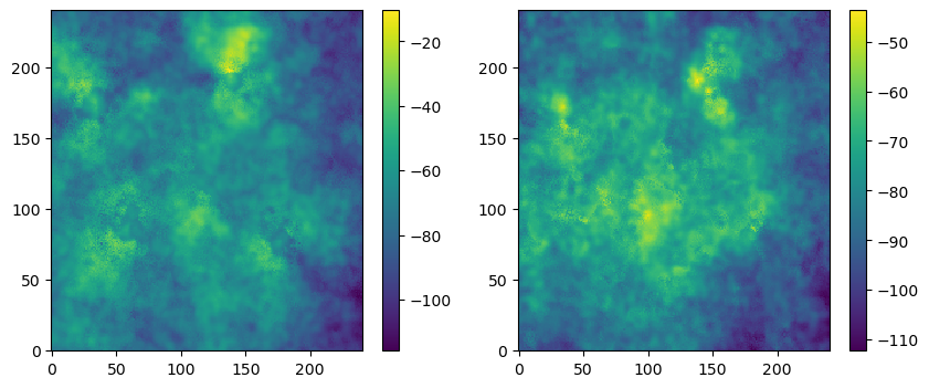
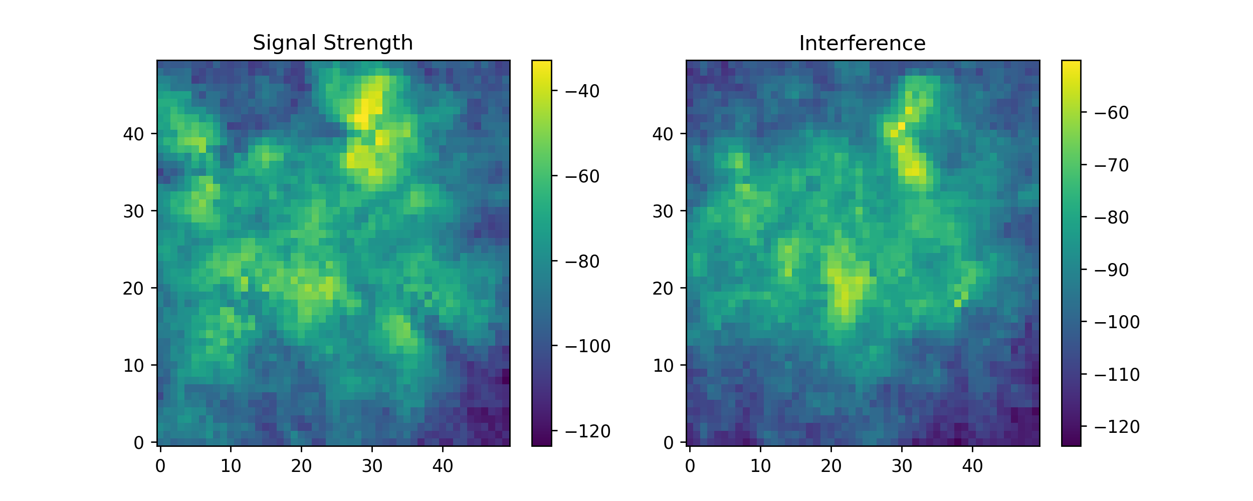
In this paper, we consider composite BO cases where is a finite-dimensional space and is a space of continuous functions. That is, is a complex function for which obtaining data is expensive and is a known and cheap-to-compute functional. As an example, consider the problem of optimizing the coverage area and interference of the service provided by a set of cell towers[29]. In this case, encodes possible configurations of antenna transmission powers and down-tilt angles of 15 different cell towers, while is the function that outputs the signal power and interference strength, respectively, at any desired location in . An example plot for signal strength and interference intensity is shown in Figure 1. Finally, uses this map to compute a score that evaluates the quality of coverage and extent of interference between towers. In this scenario, predicting the map of signal strength/interference is a challenging problem involving complex physics, while computing given this map is a simple and computationally cheap task. For problems like this, it is possible to use operator learning to infer the map from data and use composite BO to determine the best configuration for antenna powers and down-tilt angles. We explore this particular problem, among others, in our experiments section.
The choice of using traditional or composite BO is problem dependent and entails different trade-offs. If no compositional structure is known, and is completely black-box, traditional BO is the only possible approach. However, when information about the structure of allows for the formulation in the manner prescribed by the composite BO framework, studies show that the composite BO formulation achieves better results and faster convergence[27, 30].
| Paradigm | Maps | Known | Unknown - Must be Modeled |
|---|---|---|---|
| Traditional BO | N/A | ||
| Composite BO | |||
| Operator Composite BO |
2.2 Epistemic Neural Networks as a Flexible Framework for Uncertainty-Aware Models
The Epistemic Neural Networks (ENNs) [17] framework is a flexible formal setup that describes many existing methods of uncertainty estimation such as Bayesian Neural Networks (BNNs) [2], dropout [20] and Deep Ensembles [3]. An ENN with parameters takes as input a feature vector along with a random index and outputs a prediction . Under this framework, the random index is sampled from probability distribution independently from and therefore has no connection to the data and can be varied in order to obtain different predictions.
For example, a deep ensemble with networks falls into the ENN umbrella in the following manner. The random index can take values in the discrete set , indicating which network we use to carry out the prediction. In this way, varying gives us variety of predictions which allow us to estimate uncertainty by checking how much they agree or disagree with each other. If enough data is available and the model is well trained, we expect the predictions to not depend strongly on , meaning that there is little disagreement between different networks. On the other hand, if our predictions vary a lot depending on , this indicates that there is large model (also called epistemic) uncertainty. Another example of this are Bayesian neural networks (BNNs), where the weights of the network are sampled according to a re-parametrization trick using , which in this case takes on continuous values. In [17], the authors prove that BNNs are a special case of the ENN framework.
Under this framework, we can use the same feature and vary in order to estimate the epistemic uncertainty of our model, which is crucial in the context of Bayesian Optimization.
2.2.1 EpiNets
The paper [17] also introduces EpiNets, which implements an ENN in a simple and computationally cheap manner as
| (3) |
Here, is the parameters of the base network (which does not take into account), denotes the parameters of the EpiNet, is the overall set of trainable parameters, sg is a stop gradient operation that blocks gradient back-propagation from the EpiNet to the base network, and is a function that extracts useful features from the base network, such as the last layer of activations concatenated with the original input.
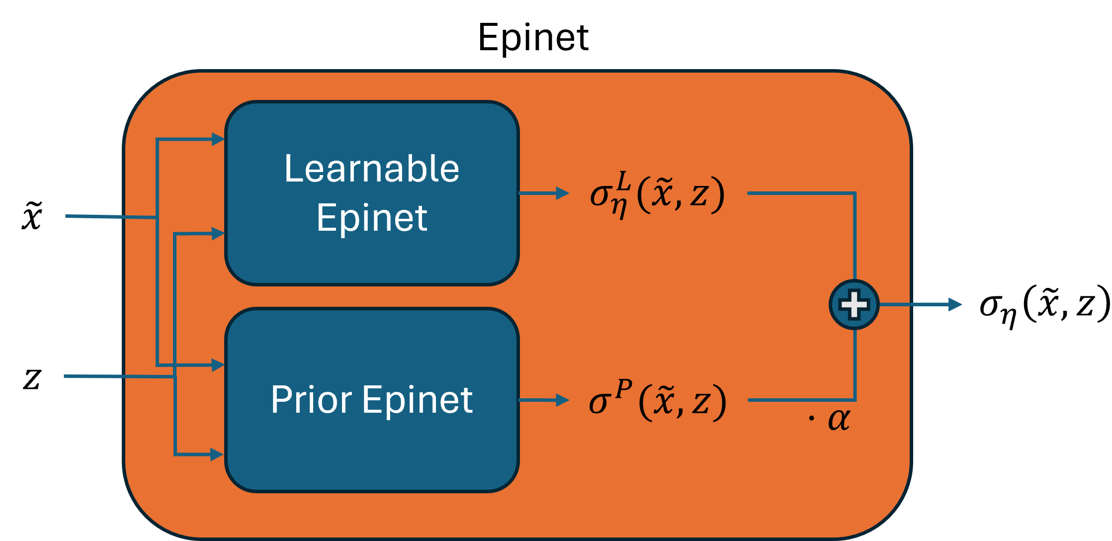
The EpiNet itself is composed of two parts, a learnable component , and a prior component which is initialized randomly and is not optimized,
| (4) |
where is a hyperparameter called the scale of the prior. Feeding the random index along with the features ensures that does in fact play a role in predictions, as the learnable component of the EpiNet has to learn to counteract the effect of the untrained prior component as opposed to making only trivial zero predictions during training.
EpiNets readily enable the quantification of epistemic uncertainty for any given neural network architecture, including any pre-trained models that can be treated as a black-box. Even for large base models with tens of millions of parameters, augmentation by a small EpiNet has been demonstrated to yield good uncertainty estimates at little extra computational cost [17]. This poses a significant advantage over deep ensembles, for example, where several models need to be trained. In addition, the EpiNet can be trained in conjunction to the base network, or at a later stage, after the base network has been trained and its parameters fixed. This yields further flexibility, as an EpiNet can be used to augment any pre-trained base network, even if it does not originally fit into the ENN umbrella.
2.3 Epistemic Operator Networks as Surrogate Models
Given an unknown function , we assume an epistemic model, which, given inputs and parameters , computes predictions , where is a feature vector, is a query point and is a random epistemic index with probability distribution over the space . Given and , the predictive distribution for the unknown quantity is equal to that of the transformed random variable where . That is, draws from the predictive distribution of can be obtained by first sampling and then computing the forward pass .
Alternatively, if the output of is a probability distribution itself (in cases such as ones using Negative Log-Likelihood (NLL) loss), instead of a single point in we model our predictive distribution for as a mixture of the output of the model over different values of
| (5) |
This implies our predictive distribution over the objective function is
| (6) |
Although we do not take this approach in the experiments considered in this paper, training a model in this manner further allows for disentangling aleatoric and epistemic uncertainty and is the potential subject of future research.
2.4 NEON - An Architecture for Epistemic Operator Learning
NEON (Neural Epistemic Operator Network) is a combination of the operator learning framework[21, 4, 5] with the EpiNet[17] architecture. More specifically, it is a version of the EpiNet architecture where the base network is an operator learning model.
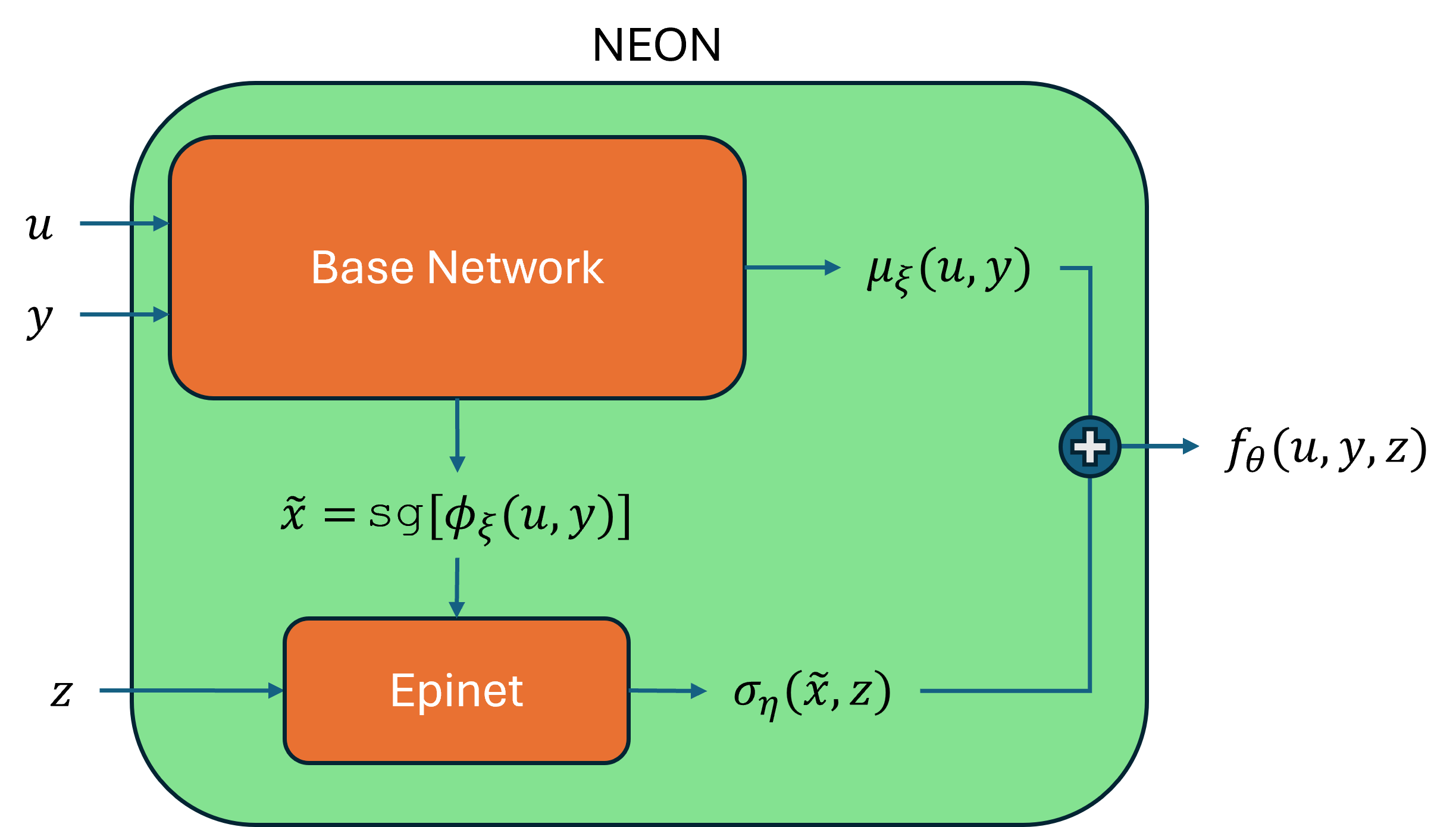
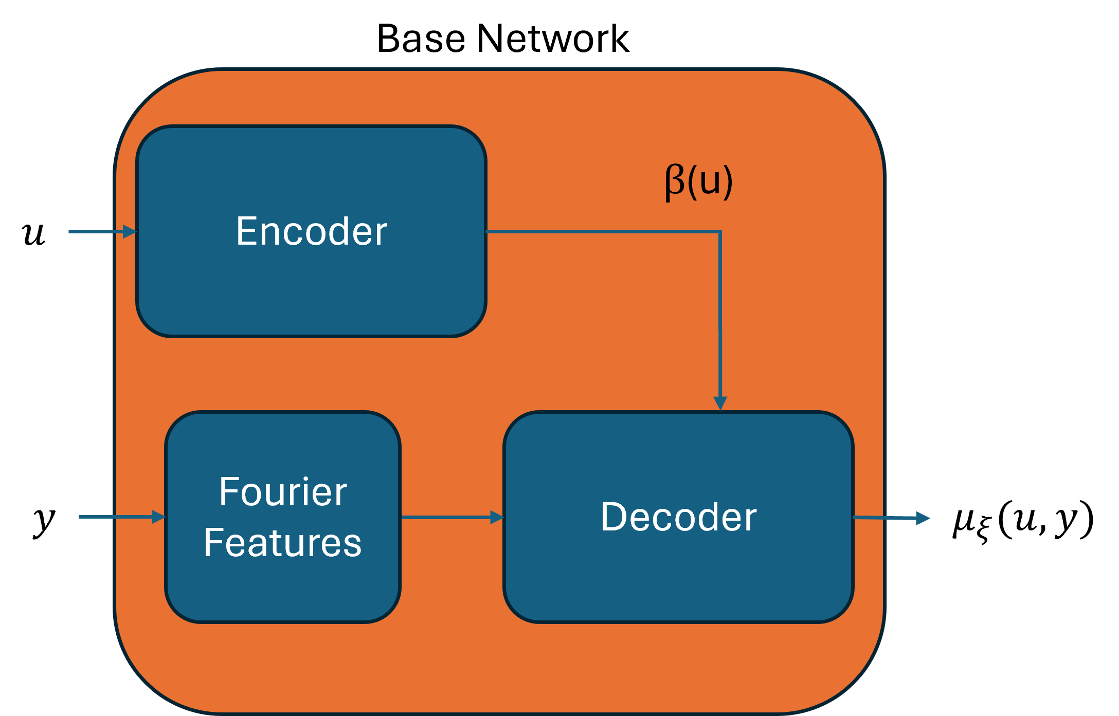
The operator learning architectures used as base networks in this paper follow a encoder/decoder structure, where the encoder with parameters takes in as input and outputs a latent variable , and the decoder with parameters takes as input and a query point and outputs the prediction . Thus, the base network makes predictions of the form , where are the trainable parameters. In the experiments considered in this paper, the encoder is a Multi-Layer Perceptron (MLP), while the decoder is either another MLP taking as input a concatenation of and a Fourier-Feature[31] encoding of , or a Split Decoder, which is an architecture inspired by [32] and further described below. Despite these specific choices, NEON can use any other choice of architecture for the backbone of the encoder or decoder.
As for the architectures of the EpiNets, we use MLPs, which take as input and , where sg is the stop gradient operation, which stops backpropagation from the EpiNet to the base network during training. In the architectures implemented in this paper, we take to be the concatenation , where is the output of the encoder, is the last layer activations of the decoder, and is the query point. Both the trainable and prior EpiNet networks then take as input the pair . This choice is similar to the original formulation of EpiNets in [17].
A diagram illustrating this choice of architecture can be seen in Figure 2, and details about hyperparameters used for each experiment can be seen in the appendix.
2.4.1 Decoder Architectures
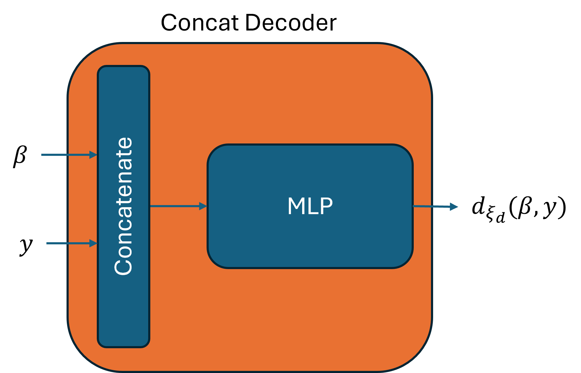
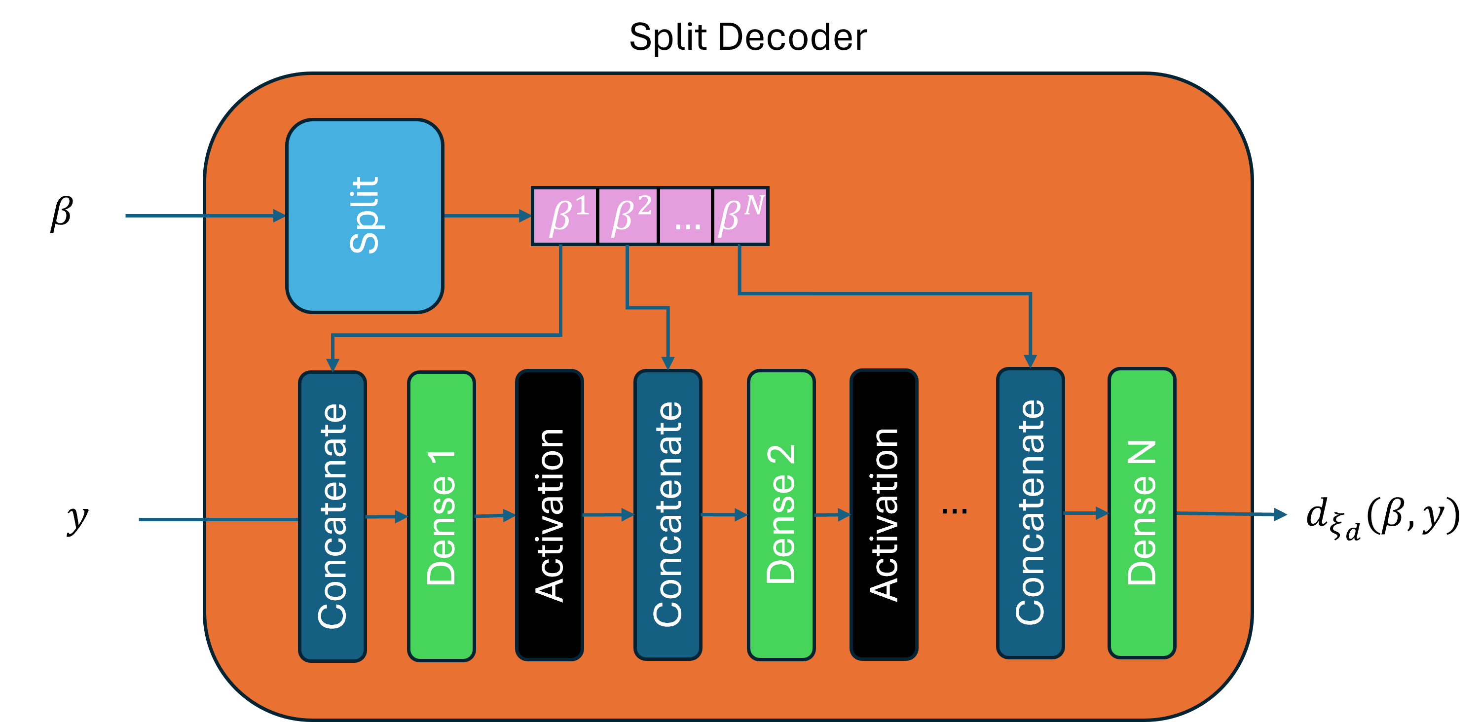
The basic formulation of NEON entails base networks that follows an encoder/decoder structure , where are the trainable parameters of the encoder and decoder, respectively. Although NEON allows for many different choices of architecture for the encoder and decoder, in the experiments carried out in this paper encoders are always MLPs, while decoders are either Concat Decoders or Split Decoders, which are described in this section and illustrated in Figure 3. Other reasonable choices would be convolutional network or a Fourier Neural Operator (FNO)[5] for the encoder, and attention-based decoders[7, 32].
The simpler among the two decoders we used, Concat Decoder is defined by the concatenation of the latent representation of the input function with a Fourier feature encoding of the query point . Although this architecture yields good results on simpler tasks, it may under-perform in cases where a larger latent dimension is needed [32]. This would be the case when the target output function concentrate on a high-dimensional nonlinear manifold [21].
The Split Decoder approach, inspired by [32], instead splits into smaller components where . These are then used to modulate the features of each hidden layer in the decoder. This approach helped the authors better fit the data by having the hyperparameter be larger than it otherwise would be able to. This larger value of allowed the encoder to preserve more information about the input function and create a richer latent representation.
2.5 Bayesian Optimization Acquisition Functions
In this section we examine some possible choices for the acquisition function used in BO. As previously described, BO aims to optimize a black-box function . Given a trained epistemic model , different choices of acquisition function can be made. In the case of Operator Composite BO, we have that , where is a known and cheap-to-evaluate functional and is a neural epistemic operator network trained on the available data.
Popular choices in the literature are Expected Improvement (EI), Probability of Improvement (PI) and Lower Confidence Bound (LCB), also called Upper Confidence Bound (UCB) in the case of function minimization instead of maximization. Some of these common choices are summarized in Table 2. It should be noted that the definition of these functions is the same in both traditional and composite BO.
An important property of all the acquisition functions considered in this paper and detailed in Table 2 is that they are expectations over . That is, they can be written as , where . Therefore, we can approximate their value by averaging the quantity of interest over different epistemic indices sampled in an i.i.d. manner from . This is important, as the predictive distribution generated by is often intractable or non-analytical. Using a Monte Carlo approximation, we can obtain .
The EI acquisition function focuses on improvement over the best value acquired so far. That is, if is the data collected so far and we set , then EI is defined in terms of our belief of surpassing this value. As the name suggests, we compute the expected improvement from collecting this new point , where this is determined by the surrogate model . This can be equivalently expressed as , where is the Rectified Linear Unit function.
It is well known that functions involving ReLU often suffer from vanishing gradients[33], where its derivative is 0 in large regions of the input space. This phenomena is problematic when carrying out optimization with algorithms that use information about derivatives of a function. In particular, we’ve found that this completely prevented any meaningful optimization of the EI acquisition function in our experiments. In light of this fact, in this paper we also propose the Leaky Expected Improvement (L-EI) acquisition function, where ReLU is substituted by the LeakyReLU [34] in the formulation of . This greatly facilitates the process of determining , while maintaining similar global optima as . Thus, we obtain where
| (7) |
Since the number in the formulation of is arbitrary, this can be generalized to
| (8) |
where we substitute with an arbitrary . In cases where the subscript is omitted, we assume the default choice of . This generalization allows us to adjust the negative slope of this acquisition function and make it closer to the original formulation of expected improvement if desired. We prove in the appendix the following short theorem, which states that for any given bounded function we can make Leaky Expected Improvement as close to EI as desired, no matter the choice of surrogate model .
Theorem 1
Let and be a bounded function. Then there exists a choice of such that for any surrogate model we have that . This implies that .
To the best of the authors’ knowledge, this Leaky Expected Improvement (L-EI) acquisition function has not been presented before, but is similar in flavor to the techniques presented in [35].
The LCB acquisition function differs from EI by having a hyperparameter which explicitly controls the exploration/exploitation trade-off. The LCB acquisition function is composed of two terms: , which represents the expected value of according to our surrogate model, and , which represents the epistemic uncertainty of the prediction. It is also common to instead set . By combining these two terms under a scaling controlled by , we obtain , where a higher choice of leads to prioritizing regions of space where our predictions are most uncertain, and lower choices of lead to ignoring uncertainty and focusing on regions that have the highest mean prediction. The value of may be fixed for the entire BO process, or dependent on the iteration number . In particular, scaling leads to provable guarantees for the regret in the GP bandit setting[36].
| Acquisition Function | Hyperparameters | ENN Formulation |
|---|---|---|
| Expected Improvement (EI) | None | |
| Leaky Expected Improvement (L-EI) | ||
| Lower Confidence Bound (LCB) |
2.5.1 Optimization of Acquisition Functions
In order to carry out BO, it is necessary to compute at each iteration, which entails solving an optimization problem. As described in the previous section, values of are determined in a Monte Carlo fashion as
| (9) |
Since all models and acquisition functions considered in this paper are almost-everywhere differentiable as a function of , we optimize using the SciPy[37] implementation of the constrained Limited memory BFGS (L-BFGS) algorithm[38]. We carry out this process times using different initial points to obtain converged solutions and set the new point to be collected as . Due to the highly non-convex nature of the problems considered in this paper, is an important hyperparameter to consider, and we’ve found that setting yields good results in practice. It should also be noted that each optimization can be done independently, so the process of obtaining all the is easily parallelised.
2.5.2 Parallel Acquisition
The acquisition functions described in Table 2 assume that new points are acquired at each iteration of BO. Extensions of these methods such as -EI[39] and more[40, 41] propose to determine where at each step different inputs are acquired simultaneously. These multi-acquisition functions are also compatible with the NEON framework and an experiment in this setting is briefly explored in the appendix.
3 Results
In this section we employ our method on several synthetic and realistic benchmarks. By augmenting a deterministic operator network with a small EpiNet, thus creating NEON, we observe considerably less data and model-size requirements in order to obtain good performance. Across all experiments we observe comparable or better performance to state-of-the-art approaches, while using orders of magnitude less trainable parameters. A comparison on the total number of trainable parameter can be seen in Table 3.
In what follows, we wish to optimize a function with compositional structure where is a finite dimensional space, is an unknown map from to a space of continuous functions, and is a known and cheap-to-evaluate functional. In practice, we must evaluate the function on several points in order to compute . Although NEON allows for the evaluation of on any arbitrary point , we limit ourselves to a fixed grid in order to be compatible with the existing literature[23, 22] and provide a fair comparison. We then wish to optimize using the procedure described in the Methods section.
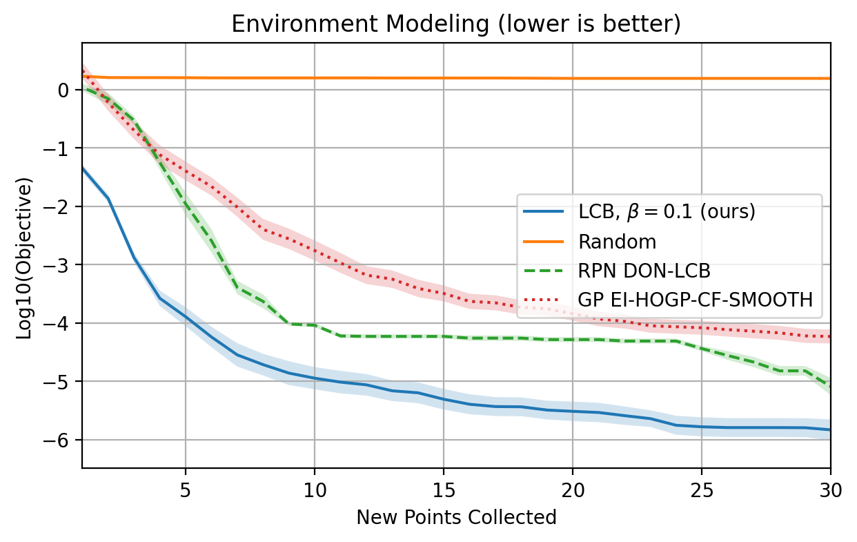
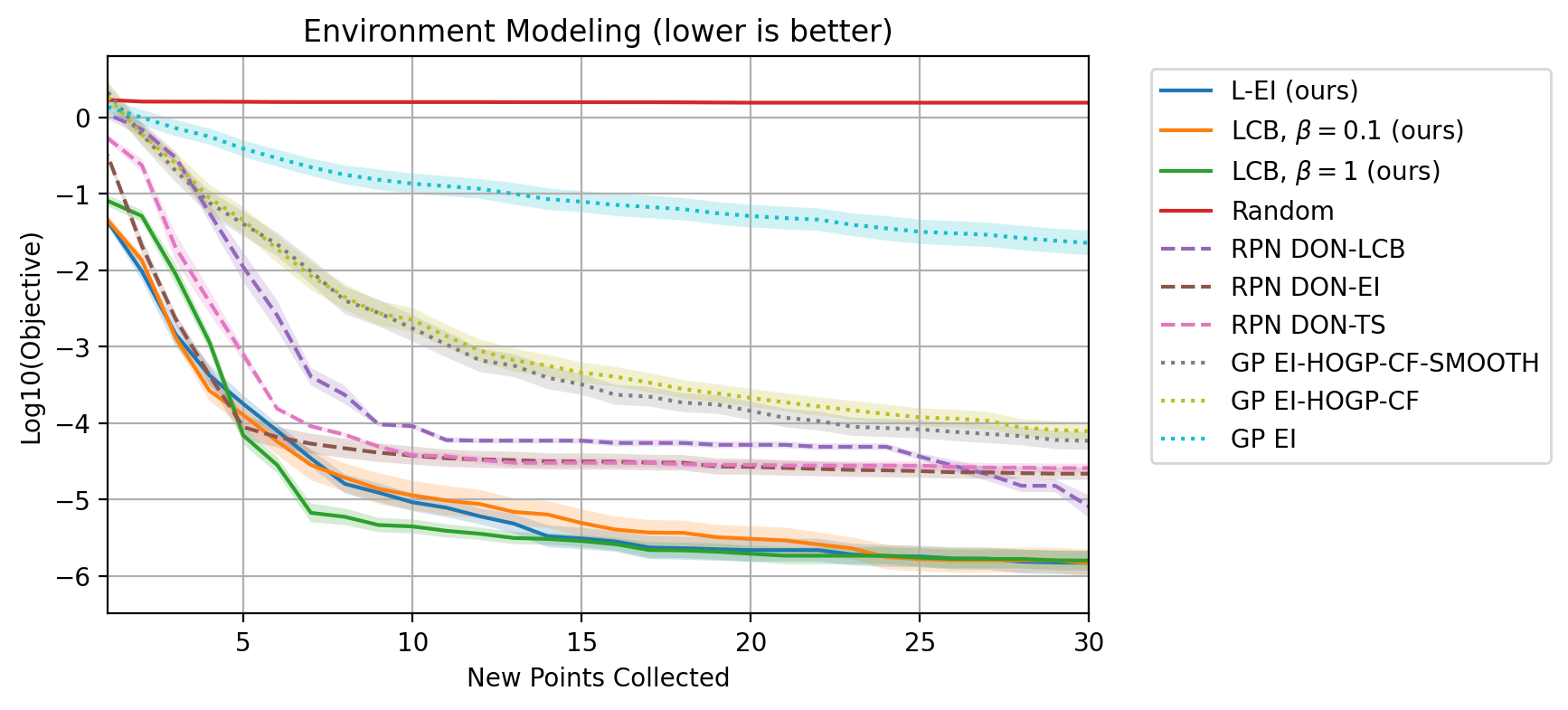
3.1 Environment Model Function
This example consists of modeling a chemical spill in a long and narrow river, and is a common synthetic benchmark in the Bayesian optimization literature[27, 22]. Given the concentration of a chemical along the river at different points in time and space, the objective of this problem is to determine the original conditions of the spills: total mass, time, position and diffusion rate. For this problem, with and , with being evaluated on a 3x4 grid on the domain . Further details about the underlying process can be found in the appendix as well as in [42, 27].
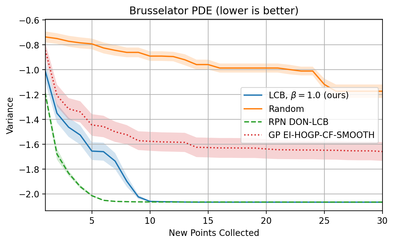
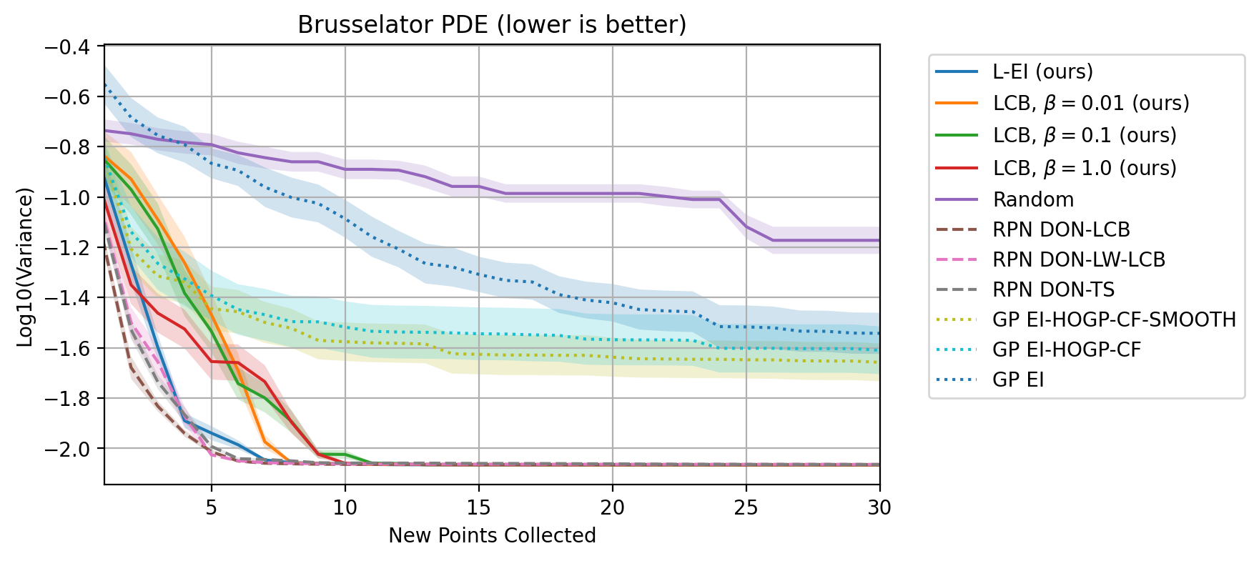
3.2 Brusselator PDE
This problem attempts to determine the optimal diffusion and reaction rate parameters to stabilize a chemical dynamical system. This dynamical system can be modeled according to a PDE described in the py-pde[43] documentation https://py-pde.readthedocs.io/en/latest/examples_gallery/pde_brusselator_expression.html. The goal is then to minimize the the weighted variance of of the solution of this PDE, which can be thought of as finding a stable configuration of the chemical reaction. For this problem, with and , with being evaluated on a 64x64 grid on the domain . Ground truth solutions are obtained via the py-pde[43] package.
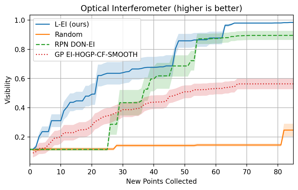
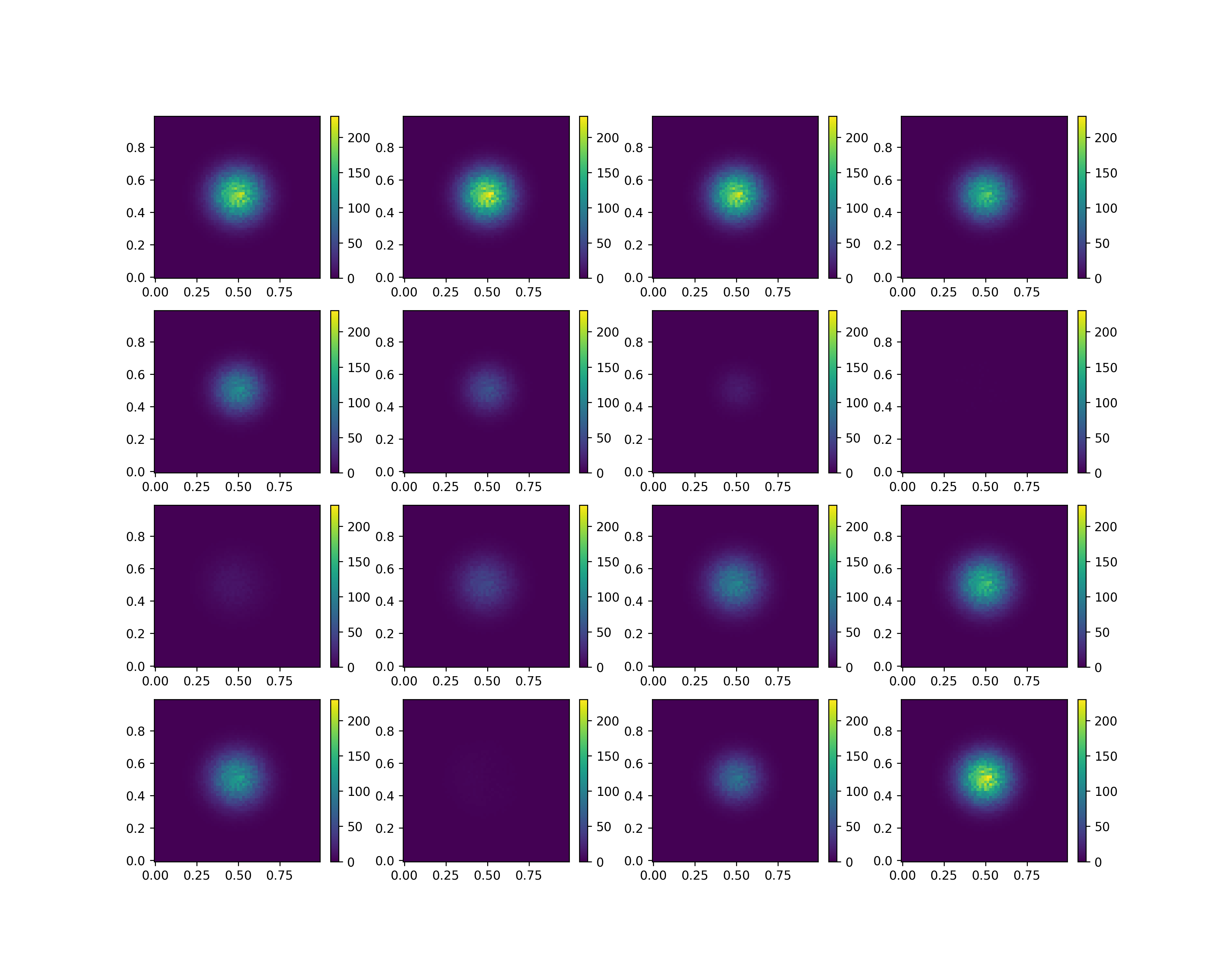
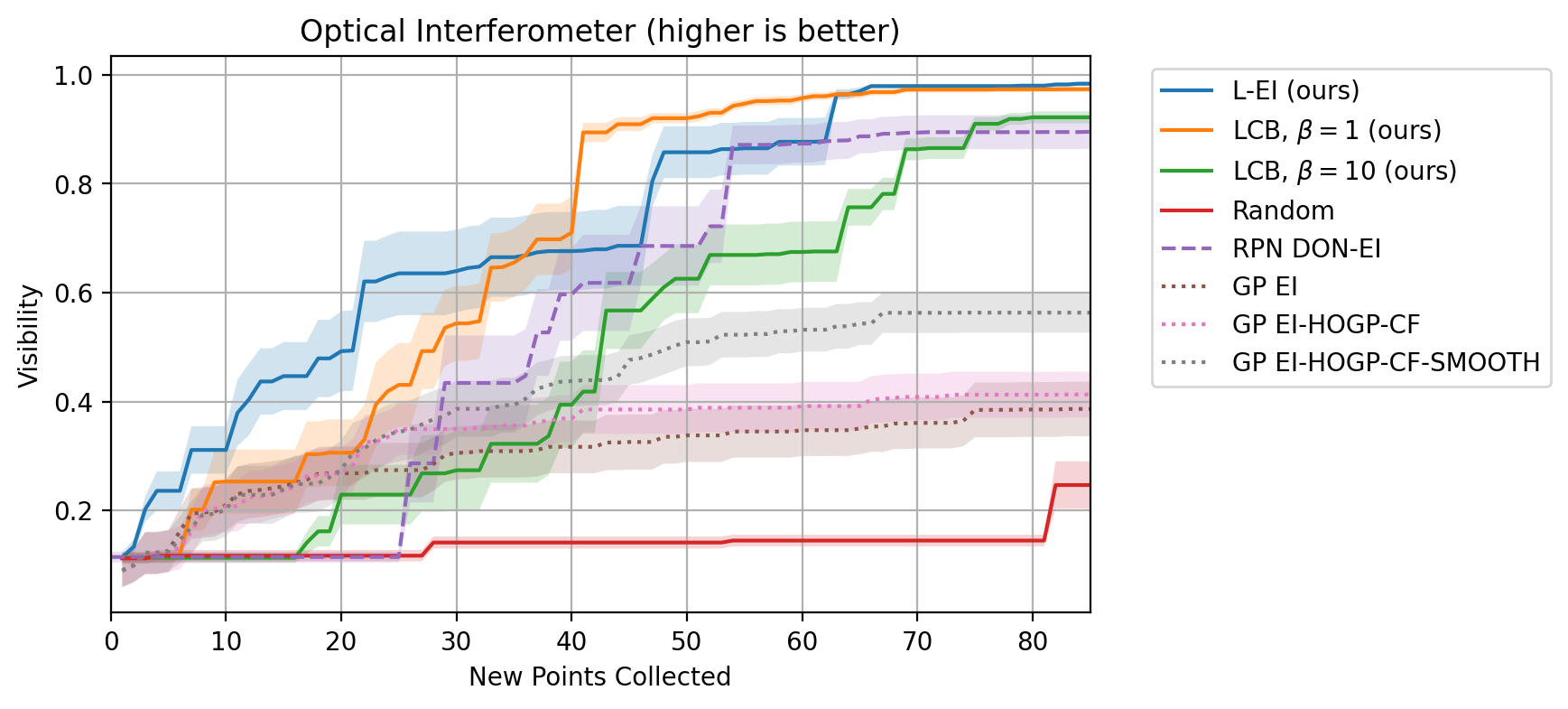
3.3 Optical Interferometer
This problem consist of aligning a Mach-Zehnder interferometer by determining the positional parameters of two mirrors in order to minimize optical interference and thus increase visibility, which is measured as defined in [44]. For this problem, with and , with being evaluated on a 64x64 grid on the domain . Ground truth solutions are obtained using the code from [44], available at https://github.com/dmitrySorokin/interferobotProject.
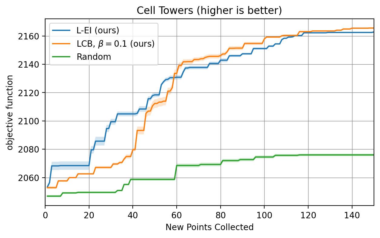
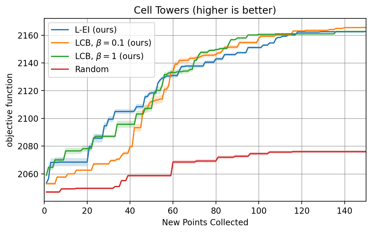
3.4 Cell Towers
This problem consists of optimizing parameters of 15 different cell service towers in order to maximize coverage area and minimize signal interference between towers. Each tower has a downtilt angle parameter lying in , as well as a power level parameter lying in , meaning that the input dimension of this problem is , with inputs . The function then uses these parameters to compute the map of coverage and interference strengths, respectively. An example of such maps can be seen in Figure 1. We compute the ground truth values of using the code presented in [29] and available at https://github.com/Ryandry1st/CCO-in-ORAN, which creates results in a grid, then downsampling to , as done in [23]. We then use the objective function presented in [23] to obtain the final score for a given set of parameters .
4 Discussion
In this paper we propose a unified framework for understanding uncertainty in operator learning and high-dimensional regression, based on the general language of Epistemic Neural Networks (ENNs). We combine ideas from ENNs and operator learning to create NEON, a general framework for epistemic uncertainty quantification in neural operators using a single backbone architecture, as opposed to an ensemble as is done in [3, 22]. NEON works by augmenting any operator network with an EpiNet, a small neural network as described in [17], which allows for easy and inexpensive quantification of epistemic uncertainty.
By carrying out numerical experiments on four different benchmarks for operator composite BO, we demonstrate NEON achieves similar or better performance to state-of-the-art methods while often using orders of magnitude less training parameters, as can be seen in Table 3.
In the more complex case of the Optical Interferometer, an ensemble of small networks is generally unable to capture the complex nature of the map . As such, we use a single larger network augmented by a small EpiNet (195,728 trainable parameters in total) instead of an ensemble of small networks as was done in [22]. This led to the biggest improvement in performance between the two methods among the cases considered. The implementation of NEON allows for the added power of a larger network while still capturing epistemic uncertainty, whereas an ensemble of equally powerful networks would present a much higher computational cost.
| ModelProblem | Pollutants | PDE Brusselator | Optical Interferometer | Cell Towers |
|---|---|---|---|---|
| NEON (ours) | 27,746 | 38,820 | 195,728 | 93,096 |
| RPN DeepONet Ensamble [22] | 1,123,072 | 1,131,264 | 45,152 | N/A |
Future research in this area may focus on finding more appropriate architectures for EpiNets carrying out UQ in high dimensions, or studying new applications to this method, such as active learning for operator networks.
Acknowledgements
We would like to acknowledge support from the US Department of Energy under the Advanced Scientific Computing Research program (grant DE-SC0024563), the US National Science Foundation (NSF) Soft AE Research Traineeship (NRT) Program (NSF grant 2152205) and the Samsung GRO Fellowship program. We also thank Shyam Sankaran for helpful feedback when reviewing the manuscript and the developers of software that enabled this research, including JAX[45], Flax[46] Matplotlib[47] and NumPy[48].
References
- [1] Carl Edward Rasmussen and Christopher K. I. Williams. Gaussian processes for machine learning. Adaptive computation and machine learning. MIT Press, 2006.
- [2] Ethan Goan and Clinton Fookes. Bayesian neural networks: An introduction and survey. In Case Studies in Applied Bayesian Data Science, pages 45–87. Springer International Publishing, 2020.
- [3] Balaji Lakshminarayanan, Alexander Pritzel, and Charles Blundell. Simple and scalable predictive uncertainty estimation using deep ensembles, 2016.
- [4] Lu Lu, Pengzhan Jin, Guofei Pang, Zhongqiang Zhang, and George Em Karniadakis. Learning nonlinear operators via DeepONet based on the universal approximation theorem of operators. Nature Machine Intelligence, 3(3):218–229, mar 2021.
- [5] Zongyi Li, Nikola Kovachki, Kamyar Azizzadenesheli, Burigede Liu, Kaushik Bhattacharya, Andrew Stuart, and Anima Anandkumar. Fourier neural operator for parametric partial differential equations, 2021.
- [6] Nikola Kovachki, Zongyi Li, Burigede Liu, Kamyar Azizzadenesheli, Kaushik Bhattacharya, Andrew Stuart, and Anima Anandkumar. Neural operator: Learning maps between function spaces with applications to pdes. Journal of Machine Learning Research, 24(89):1–97, 2023.
- [7] Georgios Kissas, Jacob H Seidman, Leonardo Ferreira Guilhoto, Victor M Preciado, George J Pappas, and Paris Perdikaris. Learning operators with coupled attention. The Journal of Machine Learning Research, 23(1):9636–9698, 2022.
- [8] Sifan Wang, Hanwen Wang, and Paris Perdikaris. Learning the solution operator of parametric partial differential equations with physics-informed deeponets. Science advances, 7(40):eabi8605, 2021.
- [9] Sifan Wang, Hanwen Wang, and Paris Perdikaris. Improved architectures and training algorithms for deep operator networks. Journal of Scientific Computing, 92(2):35, 2022.
- [10] Yibo Yang, Georgios Kissas, and Paris Perdikaris. Scalable uncertainty quantification for deep operator networks using randomized priors. Computer Methods in Applied Mechanics and Engineering, 399:115399, 2022.
- [11] Apostolos F Psaros, Xuhui Meng, Zongren Zou, Ling Guo, and George Em Karniadakis. Uncertainty quantification in scientific machine learning: Methods, metrics, and comparisons. Journal of Computational Physics, 477:111902, 2023.
- [12] Angelos Filos, Sebastian Farquhar, Aidan N. Gomez, Tim G. J. Rudner, Zachary Kenton, Lewis Smith, Milad Alizadeh, Arnoud de Kroon, and Yarin Gal. A systematic comparison of bayesian deep learning robustness in diabetic retinopathy tasks, 2019.
- [13] Andre Esteva, Brett Kuprel, Roberto A. Novoa, Justin Ko, Susan M. Swetter, Helen M. Blau, and Sebastian Thrun. Dermatologist-level classification of skin cancer with deep neural networks. Nature, 542(7639):115–118, January 2017.
- [14] Yu Huang and Yue Chen. Autonomous driving with deep learning: A survey of state-of-art technologies, 2020.
- [15] Neil Houlsby, Ferenc Huszár, Zoubin Ghahramani, and Máté Lengyel. Bayesian active learning for classification and preference learning, 2011.
- [16] Andreas Kirsch, Joost van Amersfoort, and Yarin Gal. Batchbald: Efficient and diverse batch acquisition for deep bayesian active learning, 2019.
- [17] Ian Osband, Zheng Wen, Mohammad Asghari, Morteza Ibrahimi, Xiyuan Lu, and Benjamin Van Roy. Epistemic neural networks. CoRR, abs/2107.08924, 2021.
- [18] Xilu Wang, Yaochu Jin, Sebastian Schmitt, and Markus Olhofer. Recent advances in bayesian optimization, 2022.
- [19] Maximilian Balandat, Brian Karrer, Daniel R. Jiang, Samuel Daulton, Benjamin Letham, Andrew Gordon Wilson, and Eytan Bakshy. Botorch: Programmable bayesian optimization in pytorch. CoRR, abs/1910.06403, 2019.
- [20] Yarin Gal and Zoubin Ghahramani. Dropout as a bayesian approximation: Representing model uncertainty in deep learning, 2016.
- [21] Jacob H. Seidman, Georgios Kissas, Paris Perdikaris, and George J. Pappas. Nomad: Nonlinear manifold decoders for operator learning, 2022.
- [22] Mohamed Aziz Bhouri, Michael Joly, Robert Yu, Soumalya Sarkar, and Paris Perdikaris. Scalable bayesian optimization with randomized prior networks. Computer Methods in Applied Mechanics and Engineering, 417:116428, 2023.
- [23] Wesley J Maddox, Maximilian Balandat, Andrew G Wilson, and Eytan Bakshy. Bayesian optimization with high-dimensional outputs. Advances in neural information processing systems, 34:19274–19287, 2021.
- [24] Tianping Chen and Hong Chen. Universal approximation to nonlinear operators by neural networks with arbitrary activation functions and its application to dynamical systems. IEEE Transactions on Neural Networks, 6(4):911–917, 1995.
- [25] Patricio Clark Di Leoni, Lu Lu, Charles Meneveau, George Em Karniadakis, and Tamer A Zaki. Neural operator prediction of linear instability waves in high-speed boundary layers. Journal of Computational Physics, 474:111793, 2023.
- [26] Pengzhan Jin, Shuai Meng, and Lu Lu. Mionet: Learning multiple-input operators via tensor product, 2022.
- [27] Raul Astudillo and Peter I. Frazier. Bayesian optimization of composite functions, 2019.
- [28] Natalie Maus, Zhiyuan Jerry Lin, Maximilian Balandat, and Eytan Bakshy. Joint composite latent space bayesian optimization. arXiv preprint arXiv:2311.02213, 2023.
- [29] Ryan M Dreifuerst, Samuel Daulton, Yuchen Qian, Paul Varkey, Maximilian Balandat, Sanjay Kasturia, Anoop Tomar, Ali Yazdan, Vish Ponnampalam, and Robert W Heath. Optimizing coverage and capacity in cellular networks using machine learning. In ICASSP 2021-2021 IEEE International Conference on Acoustics, Speech and Signal Processing (ICASSP), pages 8138–8142. IEEE, 2021.
- [30] Samuel Kim, Peter Y Lu, Charlotte Loh, Jamie Smith, Jasper Snoek, and Marin Soljačić. Deep learning for bayesian optimization of scientific problems with high-dimensional structure. Transactions on Machine Learning Research, 2022.
- [31] Matthew Tancik, Pratul P. Srinivasan, Ben Mildenhall, Sara Fridovich-Keil, Nithin Raghavan, Utkarsh Singhal, Ravi Ramamoorthi, Jonathan T. Barron, and Ren Ng. Fourier features let networks learn high frequency functions in low dimensional domains. NeurIPS, 2020.
- [32] Daniel Rebain, Mark J. Matthews, Kwang Moo Yi, Gopal Sharma, Dmitry Lagun, and Andrea Tagliasacchi. Attention beats concatenation for conditioning neural fields, 2022.
- [33] Razvan Pascanu, Tomás Mikolov, and Yoshua Bengio. Understanding the exploding gradient problem. CoRR, abs/1211.5063, 2012.
- [34] Andrew L Maas, Awni Y Hannun, Andrew Y Ng, et al. Rectifier nonlinearities improve neural network acoustic models. In Proc. icml, volume 30-1, page 3. Atlanta, GA, 2013.
- [35] Sebastian Ament, Samuel Daulton, David Eriksson, Maximilian Balandat, and Eytan Bakshy. Unexpected improvements to expected improvement for bayesian optimization. Advances in Neural Information Processing Systems, 36, 2024.
- [36] Niranjan Srinivas, Andreas Krause, Sham M. Kakade, and Matthias W. Seeger. Gaussian process bandits without regret: An experimental design approach. CoRR, abs/0912.3995, 2009.
- [37] Pauli Virtanen, Ralf Gommers, Travis E. Oliphant, Matt Haberland, Tyler Reddy, David Cournapeau, Evgeni Burovski, Pearu Peterson, Warren Weckesser, Jonathan Bright, Stéfan J. van der Walt, Matthew Brett, Joshua Wilson, K. Jarrod Millman, Nikolay Mayorov, Andrew R. J. Nelson, Eric Jones, Robert Kern, Eric Larson, C J Carey, İlhan Polat, Yu Feng, Eric W. Moore, Jake VanderPlas, Denis Laxalde, Josef Perktold, Robert Cimrman, Ian Henriksen, E. A. Quintero, Charles R. Harris, Anne M. Archibald, Antônio H. Ribeiro, Fabian Pedregosa, Paul van Mulbregt, and SciPy 1.0 Contributors. SciPy 1.0: Fundamental Algorithms for Scientific Computing in Python. Nature Methods, 17:261–272, 2020.
- [38] Dong C Liu and Jorge Nocedal. On the limited memory bfgs method for large scale optimization. Mathematical programming, 45(1):503–528, 1989.
- [39] David Ginsbourger, Rodolphe Le Riche, and Laurent Carraro. Kriging is well-suited to parallelize optimization. In Computational intelligence in expensive optimization problems, pages 131–162. Springer, 2010.
- [40] Samuel Daulton, Maximilian Balandat, and Eytan Bakshy. Differentiable expected hypervolume improvement for parallel multi-objective bayesian optimization. Advances in Neural Information Processing Systems, 33:9851–9864, 2020.
- [41] Jialei Wang, Scott C Clark, Eric Liu, and Peter I Frazier. Parallel bayesian global optimization of expensive functions. arXiv preprint arXiv:1602.05149, 2016.
- [42] Nikolay Bliznyuk, David Ruppert, Christine Shoemaker, Rommel Regis, Stefan Wild, and Pradeep Mugunthan. Bayesian calibration and uncertainty analysis for computationally expensive models using optimization and radial basis function approximation. Journal of Computational and Graphical Statistics, 17(2):270–294, 2008.
- [43] David Zwicker. py-pde: A python package for solving partial differential equations. Journal of Open Source Software, 5(48):2158, 2020.
- [44] Dmitry Sorokin, Alexander Ulanov, Ekaterina Sazhina, and Alexander Lvovsky. Interferobot: aligning an optical interferometer by a reinforcement learning agent, 2021.
- [45] James Bradbury, Roy Frostig, Peter Hawkins, Matthew James Johnson, Chris Leary, Dougal Maclaurin, George Necula, Adam Paszke, Jake VanderPlas, Skye Wanderman-Milne, and Qiao Zhang. JAX: composable transformations of Python+NumPy programs, 2018.
- [46] Jonathan Heek, Anselm Levskaya, Avital Oliver, Marvin Ritter, Bertrand Rondepierre, Andreas Steiner, and Marc van Zee. Flax: A neural network library and ecosystem for JAX, 2023.
- [47] J. D. Hunter. Matplotlib: A 2d graphics environment. Computing in Science & Engineering, 9(3):90–95, 2007.
- [48] Charles R. Harris, K. Jarrod Millman, Stéfan J. van der Walt, Ralf Gommers, Pauli Virtanen, David Cournapeau, Eric Wieser, Julian Taylor, Sebastian Berg, Nathaniel J. Smith, Robert Kern, Matti Picus, Stephan Hoyer, Marten H. van Kerkwijk, Matthew Brett, Allan Haldane, Jaime Fernández del Río, Mark Wiebe, Pearu Peterson, Pierre Gérard-Marchant, Kevin Sheppard, Tyler Reddy, Warren Weckesser, Hameer Abbasi, Christoph Gohlke, and Travis E. Oliphant. Array programming with NumPy. Nature, 585(7825):357–362, September 2020.
- [49] Nikolay Bliznyuk, David Ruppert, Christine Shoemaker, Rommel Regis, Stefan Wild, and Pradeep Mugunthan. Bayesian calibration and uncertainty analysis for computationally expensive models using optimization and radial basis function approximation. Journal of Computational and Graphical Statistics, 17(2):270–294, 2008.
- [50] Diederik P. Kingma and Jimmy Ba. Adam: A method for stochastic optimization, 2017.
- [51] James T. Wilson, Frank Hutter, and Marc Peter Deisenroth. Maximizing acquisition functions for bayesian optimization, 2018.
Author contributions statement
L.F.G. and P.P. conceived the methodology. L.F.G. conducted the experiments and analysed the results. P.P. provided funding and supervised this study. All authors reviewed the manuscript.
Competing Interests Statement
To the best of the author’s knowledge, they have no competing interests related to this research.
Data Availability Statement
At the time of this preprint, the data and code used in this paper is available upon request to the authors.
5 Proof of Theorem 1
Since is bounded, there exists such that for all . If we now define and set any we have that
Additionally, if we assume that is any epistemic model with range within the accepted range of , we get that and therefore
which proves the first statement of the theorem. Finally, we have that
which concludes the proof.
6 Further Experimental Details
6.1 Environmental Model Function
As mentioned in the main text, this is an inverse problem which models two chemical pollutant spills in a long and narrow river. Given observations of the chemical concentration at certain points in time and space, the objective of this problem is to determine the initial conditions of the spill. This is a common toy benchmark for composite BO[27, 23, 22] following the formulation described in [49].
The true values for the map are given by
where is the pollutant mass spilled at each location, is the diffusion rate of the chemical in water, is the location of the second spill relative to the first one and is the time of the second spill relative to the first one.
Using the true parameters , the objective of this problem is to determine this value from observations of the chemical concentrations at positions for times .
The NEON architecture for this experiment used an MLP encoder with 2 hidden layers with hidden dimension 64 and . We used a Split Decoder with 2 layers of hidden dimension 64. The EpiNet architecture we used consisted of a trainable MLP with two hidden layers of dimension 32, and for the prior component an ensemble of 16 MLPs with 2 hidden layers of width 5 each and a scale parameter of 0.75. We trained this network for 12,000 steps using a batch size of 256 and the Adam[50] optimizer and exponential learning rate decay.
6.2 Brusselator PDE
The PDE considered in this experiment describes the chemical reaction over time of two compounds and
where are the diffusivity parameters of chemicals and , respectively, and are their reaction rates.
The tuple is the quantity we wish to minimize over in order to obtain the smallest value for the objective, which is the weighted variance of the system, determining by evolving the PDE from to using the example implementation of the PyPDE[43] package.
The NEON architecture for this experiment used an MLP encoder with 2 hidden layers with hidden dimension 64 and . We used a Split Decoder with 3 layers of hidden dimension 64 and Fourier features with a scale parameter of 5. The EpiNet architecture we used consisted of a trainable MLP with two hidden layers of dimension 32, and for the prior component an ensemble of 16 MLPs with 2 hidden layers of width 5 each and a scale parameter of 1. We trained this network for 4,000 steps using full batch and the Adam[50] optimizer and exponential learning rate decay.
6.3 Optical Interferometer
This problem consists of optimizing the positional parameters of two mirrors in order to increase visibility. The input is used to compute the interference pattern, which is a set of 16 images on , using a 64x64 grid. Thus, is the unknown ground truth map, determined in our experiments using the InterferBot package[44].
The objective function we aim to maximize is the visibility of , defined by the map
where and and
The NEON architecture for this experiment used an MLP encoder with 4 hidden layers with hidden dimension 64 and . We used a Split Decoder with 6 layers of hidden dimension 128 and Fourier features with a scale parameter of 10. The EpiNet architecture we used consisted of a trainable MLP with 3 hidden layers of dimension 64, and for the prior component an ensemble of 16 MLPs with 2 hidden layers of width 8 each and a scale parameter of 1. We trained this network for 15,000 steps using a batch size of 16,384 and the Adam[50] optimizer and linear warm up of the learning rate, followed by cosine decay.
6.4 Cell Towers
Given inputs encoding antenna down-tilt angles and transmission strength, computes the signal strength and interference, respectively, of cellular service in the area. The objective we wish to optimize is then defined as the continuous version of the objective in [23] as:
where is evaluated on a 50x50 grid and and are the weak and strong coverage thresholds, respectively.
The authors would like to point out the discrepancy between the objective function values we’ve obtained for this problem and those reported on [23]. We have reached out to the authors of [23] and they have indicated this arises from different versions of the simulation for the ground-truth function , although the objective function used was identical. Since their version of is not publicly available, we used the simulator from [29] to compute the map .
The NEON architecture for this experiment used an MLP encoder with 1 hidden layers with hidden dimension 64 and . We used a Split Decoder with 6 layers of hidden dimension 64 and Fourier features with a scale parameter of 15. The EpiNet architecture we used consisted of a trainable MLP with 3 hidden layers of dimension 64, and for the prior component an ensemble of 16 MLPs with 2 hidden layers of width 5 each and a scale parameter of 0.5. We trained this network for 12,000 steps using a batch size of 2,500 and the Adam[50] optimizer and linear warm up of the learning rate, followed by cosine decay.
7 Parallel Acquisition
In BO, it is possible to consider the problem of acquiring several new points at each iteration. This is done by selecting the points where is a multi-point (or parallel) acquisition function. This may be desirable in situations where collecting a new data point is equally costly as acquiring . For example, if an experiment requires harvesting cells from live animals, sacrificing a mouse may yield enough cells to perform several experiments simultaneously. In this case, the expensive component of evaluating the map is sacrificing the animal, but after doing so, performing a single experiment is approximately equal to performing ones. In addition to cases such as this, parallel acquisition also requires training surrogate models less times, as we only need to train one network in order to collect points at each iteration. Many single point acquisition functions have been extended to this parallel setting[39, 51], and this framework is also compatible with NEON.
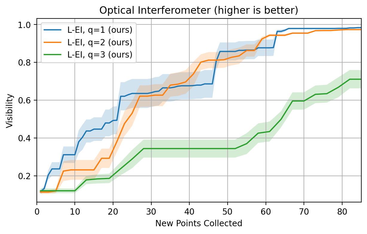
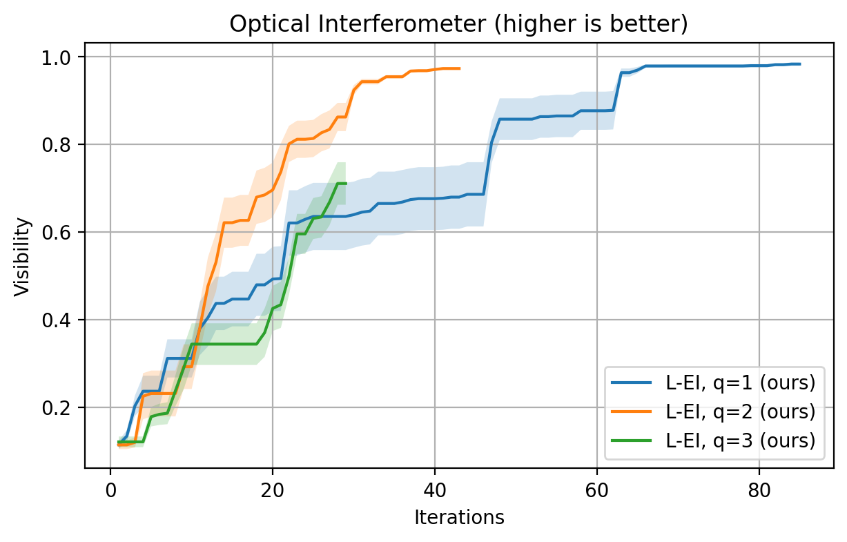
It has been shown that having quality measures of joint predictions is critical for decision making processes and that EpiNets excel at this task[17]. This makes EpiNet based architectures such as NEON good candidates for parallel acquisition problems. We validate this claim by examining the performance of NEON in the Optical Interferometer problem using -LEI, a generalization of the L-EI for parallel acquisition analogous to -EI[39]. As such, where
with
As was done in L-EI, the value can be substituted by any other if desired. This leads to an analogous statement to Theorem 1 for the parallel acquisition setting, with similar proof.
The experimental results over 5 independent trials using different seeds are presented in Figure 10. As can be seen, using with the -LEI acquisition yields similar results to the single-point acquisition function in terms of new points collected, and far superior in terms of BO iterations. Using yields slightly worse performance, but it is still able to optimize the objective function.