tcb@breakable
Robust Federated Learning for Wireless Networks:
A Demonstration with Channel Estimation
Abstract
Federated learning (FL) offers a privacy-preserving collaborative approach for training models in wireless networks, with channel estimation emerging as a promising application. Despite extensive studies on FL-empowered channel estimation, the security concerns associated with FL require meticulous attention. In a scenario where small base stations (SBSs) serve as local models trained on cached data, and a macro base station (MBS) functions as the global model setting, an attacker can exploit the vulnerability of FL, launching attacks with various adversarial attacks or deployment tactics. In this paper, we analyze such vulnerabilities, corresponding solutions were brought forth, and validated through simulation.
Index Terms:
Federated learning, incremental learning, channel estimation, adversarial attack, data poisoning.I Introduction
Federated learning (FL) empowers devices to collectively train a global model without sharing raw data, a crucial aspect for maintaining user data confidentiality in wireless networks [1]. On-device computing units, such as TrueNorth and Snapdragon neural processors, further enable FL with the necessary hardware solutions [2]. Retaining data at its origin and employing on-device learning enable swift responses to real-time events in latency-sensitive applications. FL is recognized as a promising enhancement for wireless networks in various aspects, such as resource allocation [3, 4] as well as beamforming design [5]. On the other hand, the global shift towards higher frequencies, attributed to their abundant spectrum resources, will raise new challenges. For instance, compared to sub-6GHz systems, millimeter-wave (mmWave) systems face a more complex environment, characterized by higher scattering, penetration losses, and path loss for fixed transmitter and receiver gain [6]. Especially, due to significantly shorter channel coherent time, conventional channel estimation techniques become impractical. Machine learning (ML) based channel estimation techniques have demonstrated their effectiveness in improving estimation performance, as well as reducing the estimation time [7].
Given the inherent high dynamics of high-frequency radio channels, which can exhibit diverse characteristics across varying weather conditions, timely model updates based on real-time data are crucial. With FL, the model can undergo rapid updates without substantial communication overhead. Meanwhile, the training will be carried out parallel, further reducing the update time. While compelling, many recent studies involve training local models with edge devices, followed by the base station receiving and aggregating model updates to update the global model [6, 8, 9]. On-device training reduces communication overhead, yet synchronizing diverse edge devices on large-scale, particularly on resource-constrained mobile user (MU), poses a significant challenge. Thus, effort have been made towards small base station (SBS) level training, with the SBSs training on a small dataset cached from nearby MUs, and the model aggregation is performed on a macro base station (MBS) [10, 11]. This FL strategy aims to provide more reliable and timely model updates. Most recently, research focus have been shifted to scenarios where both base station (BS) and edge devices are capable of training local models, and the aggregation is performed on the BS [12, 13].
Threats of FL-based channel estimation can be categorized in two aspects: i) malicious local models providing malicious model updates ii) data from poisoned sources. In BS-based training, compromising a BS into a malicious local model is unlikely, yet the security concern persists with the vulnerability to poisoned data sources. However, there is still overlap between security concern of those frameworks. In instances of data poisoning, an attacker may deploy a substantial set of malicious MU to execute data poisoning attacks on a specific BS. In such scenarios, the impact is akin to involving a malicious local model.
In this work we consider data poisoning attacks on SBS. The attacks may launch widely, or target in one specific SBS, mirroring scenarios involving malicious local models. Firstly, we evaluate the vulnerability to adversarial attacks on channel estimation models. Secondly, we propose novel aggregation functions leveraging Bayesian Model Ensemble (BME), which ensures resilience against attacks without compromising estimation performance. Thirdly, we employ a pre-filtering strategy based on local loss distribution to mitigate attacks that are widely launched. Our simulation results highlight the effectiveness of our methods in mitigating diverse attacks, surpassing conventional approaches, and offering insights to bolster the security and resilience of FL in wireless communication.
II Preliminaries
II-A Channel estimation model
ML-based models are trained with algorithms to learn underlying patterns and correlations in data, subsequently enabling them to predict patterns in new data. The channel estimation model can be described as follows,
| (1) |
where represents the input pilot signal, takes the form of a matrix . The output signifies the estimation result of the channel estimation model, with denoting the predicted Channel state information (CSI) matrix. The parameter corresponds to the weights of the channel estimation model.
By integrating FL, we can refine the model by fine-tuning it using cached datasets, denoted as , where represents the number of SBS and denotes the federation round. At each federation round, local models undergo steps of stochastic gradient descend (SGD), defined by the update rule:
| (2) |
where is the model weights for each local model, and is the loss function. and denote the step size and mini-batch at step, respectively, with .
II-B Robust model aggregation
Following the fine-tuning of the local model, the weight updates, denoted as , are aggregated to create a new global model with weight . The standard aggregation function, FedAvg, can be described as follows:
| (3) |
where denotes the cached dataset length at the local model. Considering FedAvg’s sensitivity to corrupted weights, robust aggregation function (RAF) is designed by exploring alternatives to the mean [14]. Common approaches for robust aggregation are exemplified here:
-
•
Trimmed Mean: In this approach, a parameter is chosen. Subsequently, the server eliminates the lowest values and the highest values and then computed from the remaining values, is then modified as , with
(4) -
•
FedMedian: Instead of averaging weights, FedMedian utilizes a median computation,
(5)
Through the use of RAFs, the global model effectively filters out potential malicious model updates. As demonstrated in [15], the Trimmed Mean method requires awareness of attacks, more specifically, the count of local models under attack, and its effectiveness varies across different attack modes. On the other hand, the FedMedian excels in resilience against various attacks. Despite these strengths, RAFs generally have a drawback: the potential to discard usefull model updates, which leads to inferior convergence performance compared to FedAvg. To address this limitation, Campos et al. proposed a dynamic framework, that alternates between FedAvg and RAFs for a better convergence than simply employing RAFs [14].
III Threat model
In the above described channel estimation scenario, we contemplate the presence of a certain number of adversary entities (AEs). These AEs strategically launching attacks on one or several SBSs. The objective is to manipulate the global model through the aggregation process. Launching attacks on all SBSs demands significant resources. However, with the advent of unmanned aerial vehicle (UAV) as potential attack platforms, the feasibility of attacks on the majority or entirety of SBSs can’t be ignored. Considering that the model transmission is exclusively between SBS and MBS, the use of dedicated links can effectively mitigate man-in-the-middle (MITM) attacks in the SBSs level. This attack can be done through the deployment of malicious MUs or MITM attack agents between the MUs and the SBSs. We consider the following attack modes:
III-1 Outdate mode
AEs provide random outdated CSI without any modification. In the case of MITM attack, the attack agent is required to store the outdated CSI and send back to SBS.
III-2 Collusion mode
AEs will provide the same CSI. This attack mode is designed to manipulate the model, potentially leading to model collapse, as well as to produce a desired outputted CSI. This attack mode doesn’t require any knowledge of CSI from the MITM attack agent.
III-3 Reverse mode
AEs will provide reversed version of the CSI, each value of CSI will be reversed regarding the mean. This attack mode requires the MITM attack agent to possess precise knowledge of the CSI and perform an additional processing step.
Given the channel estimation model is fine-tuned with dataset . The object is to minimize the loss , where is the predicted output corresponding to . A common choice for the loss function is the Mean Squared Error (MSE), defined as:
| (6) | ||||
And the average gradient with respect to the loss function and weight is given by:
| (7) |
Referring to Eq. (7), if the dataset exhibits a large variety, the effectiveness of collusion mode, capable of injecting malicious gradients towards specific , is likely to weaken. In comparison, reversing a subset of can effectively interfere with, or negate the useful gradient regardless of the dataset variety. The modified subset cached by the SBS can be described as , where represents the modified CSI through different attack modes. And represents the authentic subset.
IV Methodology
IV-A Robust aggregation function: StoMedian
The BME framework implements Bayesian inference on the server, thereby mitigating potential degradation in model performance [16]. Essentially, BME has the capacity to dynamically aggregate local models. In the scope of BME-based FL, chen et al. firstly employs client parameters to construct a stochastic filter for the aggregation of each federation round. While showcasing superior accuracy compared to FedAvg, Chen’s approach, FedBE, relies on utilizing a diagonal Gaussian distribution for the stochastic filter, with [17]
| (8) |
| (9) |
Given the sum set of all cached dataset , is posterior distribution of being learned. The output probability of can be denoted as , and integrating the outputs of all possible model:
| (10) |
BME with samples can be described:
| (11) |
| (12) |
Building upon this approach, it can be seamlessly integrated into robust aggregation techniques, ensuring system resilience without compromising convergence performance across federation rounds. However, it’s worth noting that weights in ML models are typically normalized to approach , making original approach insensitive when encountering various adversarial attacks. Hence, integrating BME into our proposed aggregation function, StoMedian, introduces two significant enhancements geared towards improving sensitivity to adversarial attacks: i) The stochastic filter was constructed using the logarithm of weights to ensure high sensitivity. ii) Rather than employing , we utilized the median of weights to mitigate the potential impact of invaded local models. The aggregation function is then presented in Alg. 1.
IV-B Local loss pre-filtering
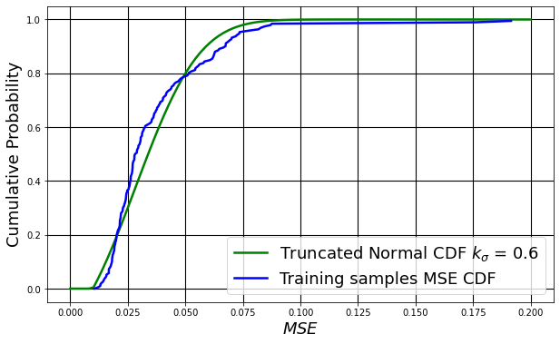
In response to potential attacks employing a widely launched strategy, where most or all local models may be impacted, a common approach is to filter the anomalies before training. Given that the global model has been pre-trained and undergoes fine-tuning during each federation round for enhanced performance, it can be utilized to identify anomalies. In a departure from the conventional use of local intrinsic dimensionality (LID) for data discrimination, we propose an alternative approach to evaluate the reliability of data originating from each MU. The loss of each sample, , where , is computed. The distribution of heavily relies on the current model and is not mathematically traceable. Therefore, we evaluate it numerically with randomly generated samples on a pre-trained model. Further details on the training setting, model specifications, and data description are provided in Section V. As depicted in Fig. 1, the cumulative distribution function (CDF) of can be accessed with CDF of a truncated Gaussian distribution with lower and upper bounds of , with
| (13) |
| (14) |
where , which is determined empirically. Similar to the approach introduced in [18], by assigning a threshold to , it is capable of detecting anomalies. Further details of the algorithm can be found in Alg. 2.
V Evaluation
V-A Model and datasets
In this work, we employ a simple Convolutional Neural Network (CNN) for channel estimation, comprising: i) an input layer ( kernel size, filters) with SeLU activation, ii) a hidden layer ( kernel size, filters) with Softplus activation, iii) an output layer ( kernel size, filter) with SeLU activation. This CNN processes input data of size and has demonstrated effective channel estimation performance, as evidenced by [19].
The datasets used for training channel estimation models were generated using a reference example titled ”Deep Learning Data Synthesis for 5G Channel Estimation,” accessible within the MATLAB 5G Toolbox, with specific settings considered. Given that pilot signals and CSI are typically represented as complex numbers, we adopted a preprocessing step. Specifically, we divided the complex data into its real and imaginary components to make it compatible with CNN. This approach aligns with prior work.
V-B Threat evaluation
The global model was initially pre-trained with a small dataset including samples. Subsequently, local models were fine-tuned with , . A validation dataset , was employed to assess the channel estimation performance, with these data never being part of the training.
To demonstrate the susceptibility of FL, we simulated our SBSs under data poisoning attacks, alongside a CL scenario as comparison. The standard FedAvg aggregation function was used. We define as an indicator of the model’s performance on seen data, as an indicator of its performance on unseen data, and as a measure of the efficacy of adversarial manipulations on the model.
We considered a minimum cached dataset length required for training. In cases where the SBS lacks sufficient data, a subset of pre-training data is appended to meet the minimum requirement. AEs can be deployed either in a widespread strategy or to target a specific SBS. The simulation setup is described in Tab I.
| Parameter | Value | Remark | |
| Number of MUs | |||
| Number of SBSs | |||
| System | Number of MBS | ||
| Number of model update rounds | |||
| Ratio of AEs | |||
| Minimum length of cached datasets required for training | |||
| Length of all cached datasets of one federation round | |||
| Length of a local cached dataset (without targeted attacks) | |||
| Length of validation dataset | |||
| Learning rate for adam optimizer | |||
| Momentum for adam optimizer | |||
| Epochs of the training | |||
| Training | Batch size |
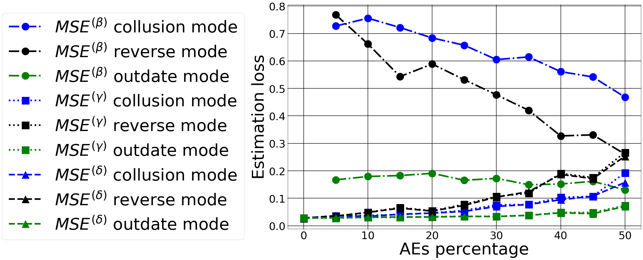
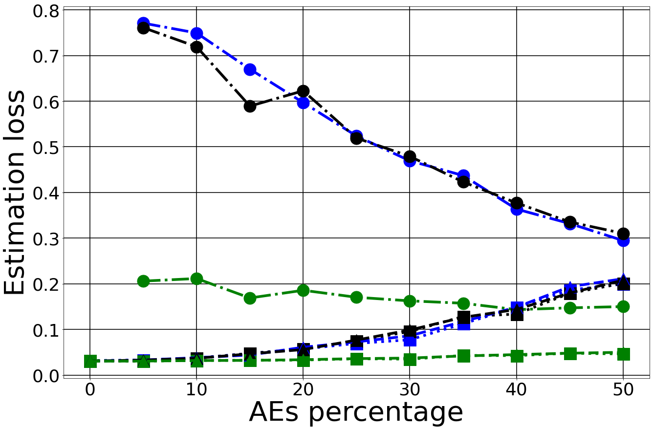
As analyzed in Section III, the reverse mode can nullify useful gradients learned from authentic data, a phenomenon whose effectiveness is confirmed by our simulation results in Figs. 2(a)–2(c). Conversely, the outdate mode has minimal impact, only slightly degrading model accuracy, due to the strong correlation between outdated CSI and actual CSI. Combining Fig. 2(a) and Fig. 2(b), FL shows significant performance degradation under collusion attacks compared to CL. This is attributed to the fact that FL trains local models on a small dataset, characterized by a limited diversity.
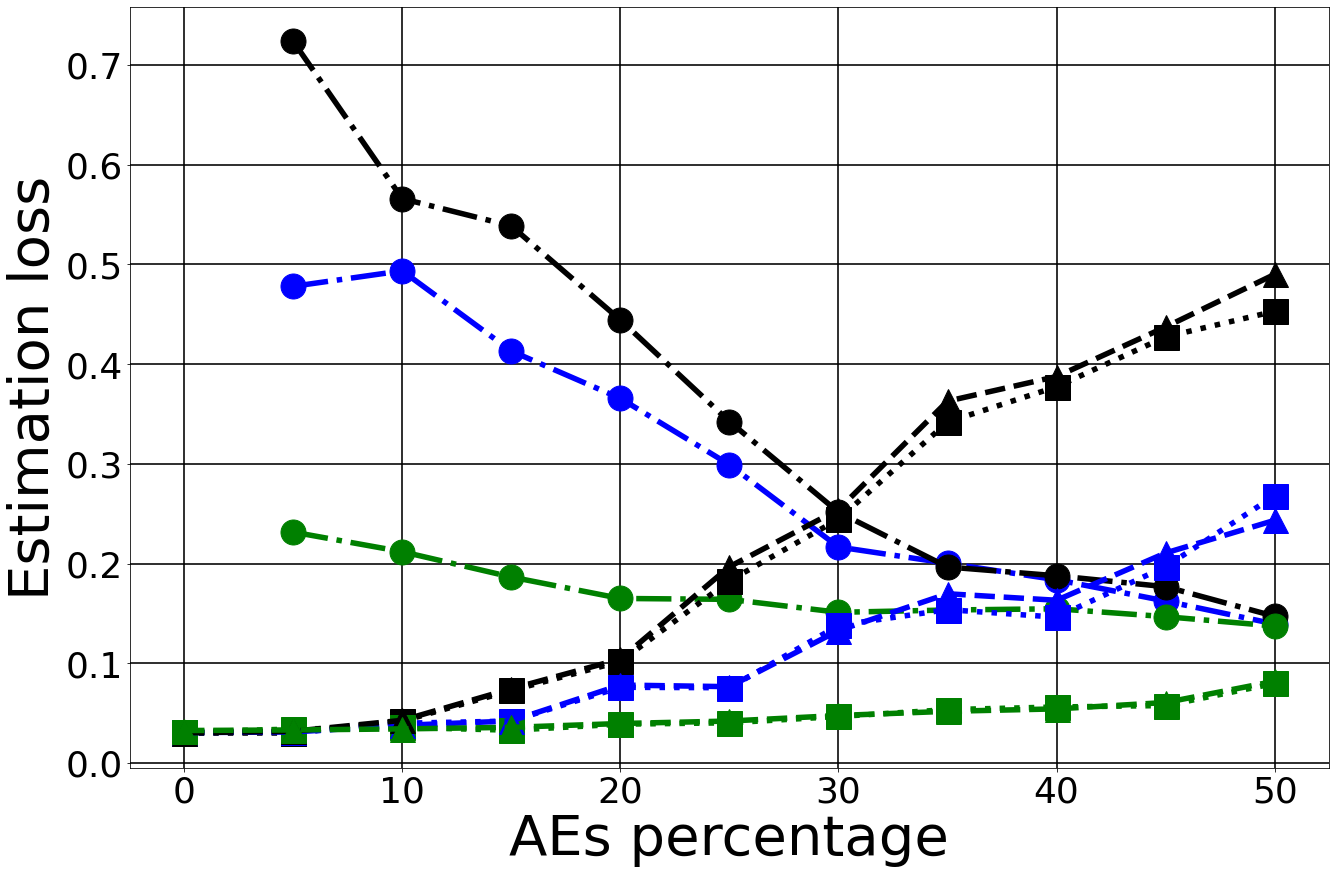
Fig. 2(c) demonstrates the vulnerability of FL to targeted data poisoning attacks on specific clients. For reverse attack, at , intersections between and either or become evident. This signifies the successful evasion of the attacker, making the attacks undetectable by the ML model itself. Meanwhile, the intersections of collusion attack appear at . Both attack modes are significantly boosted because FedAvg employs a weighted approach. This results in the victim local model, surrounded by AEs, being assigned a larger weight, further degrading model performance during aggregation. However, the efficacy of such attack strategies can be efficiently mitigated by employing RAFs.
V-C Evaluation of proposed methodology: StoMedian
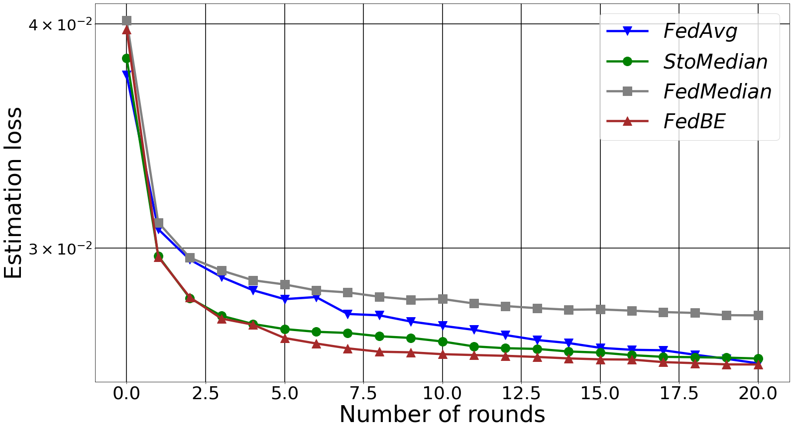
While AEs are being deployed to target a specific SBS, which is a cost-efficient and most impactful attack strategy from attacker side. To demonstrate the effectiveness of RAFs, we conducted simulations to illustrate the convergence of across federation rounds for four different aggregation functions. The simulation setup is same as listed in Tab I, with only reverse attack being considered and .
Firstly, we examine a scenario devoid of any attacks, depicted in Fig.3(a). Unsurprisingly, FedMedian demonstrates the poorest convergence performance, as we elucidated in Sec.II-B. StoMedian and FedBE demonstrated significantly superior performance compared to FedAvg, primarily due to its effectiveness in preventing model drift in the aggregation. As the overall performance improved over federation rounds, the performance gap became less evident, with all three aggregation function reaching a comparable convergence level. Meanwhile, FedBE performed slightly better than StoMedian. Nevertheless, the performance of StoMedian is contingent upon the distribution of underlying local datasets. In the worst-case scenario where local data are highly non-identically distributed, which is unlikely in our setting where SBSs have confined coverage and are not likely to exhibit diverse geographical deployments. StoMedian may filter out most local weights, resulting in convergence levels similar to that of FedMedian. In such a scenario, the performance degradation of FedAvg is inevitable.
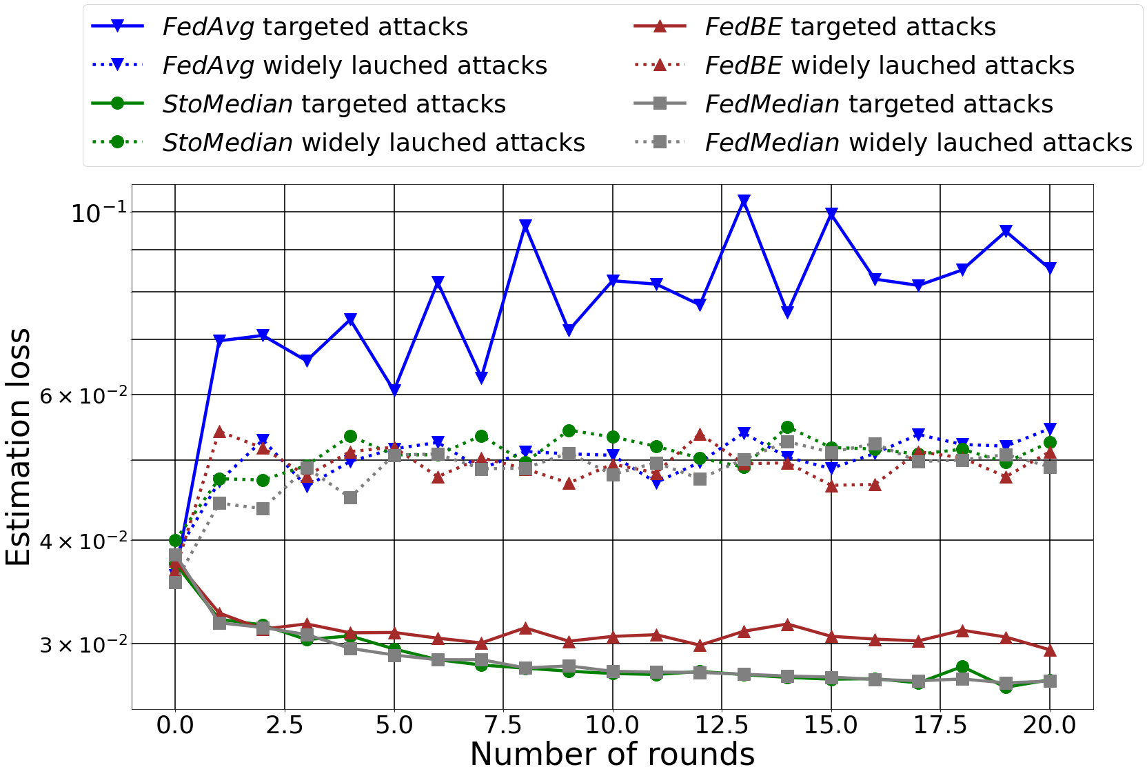
The results of convergence analysis of aggregation functions under attacks are depicted in Fig.3(b). FedAvg exhibited no defense against attacks, and FedBE demonstrated limited defense but far from resilient. The performance gap between FedBE and FedMedian is larger than that of Fig.3(a), due to the scaling which may not be immediately evident. In contrast, FedMedian and StoMedian demonstrated resilient and comparable performance against coordinated strategy. On the other hand, all aggregation functions failed to mitigate widely launched attacks effectively.
V-D Evaluation of proposed methodology: LLPF
Having evaluated the effectiveness of StoMedian, we now proceed to assess the efficacy of LLPF. The simulation setup remains consistent with the parameters outlined in Table I, with StoMedian being applied. We examine three attack modes, with set at .
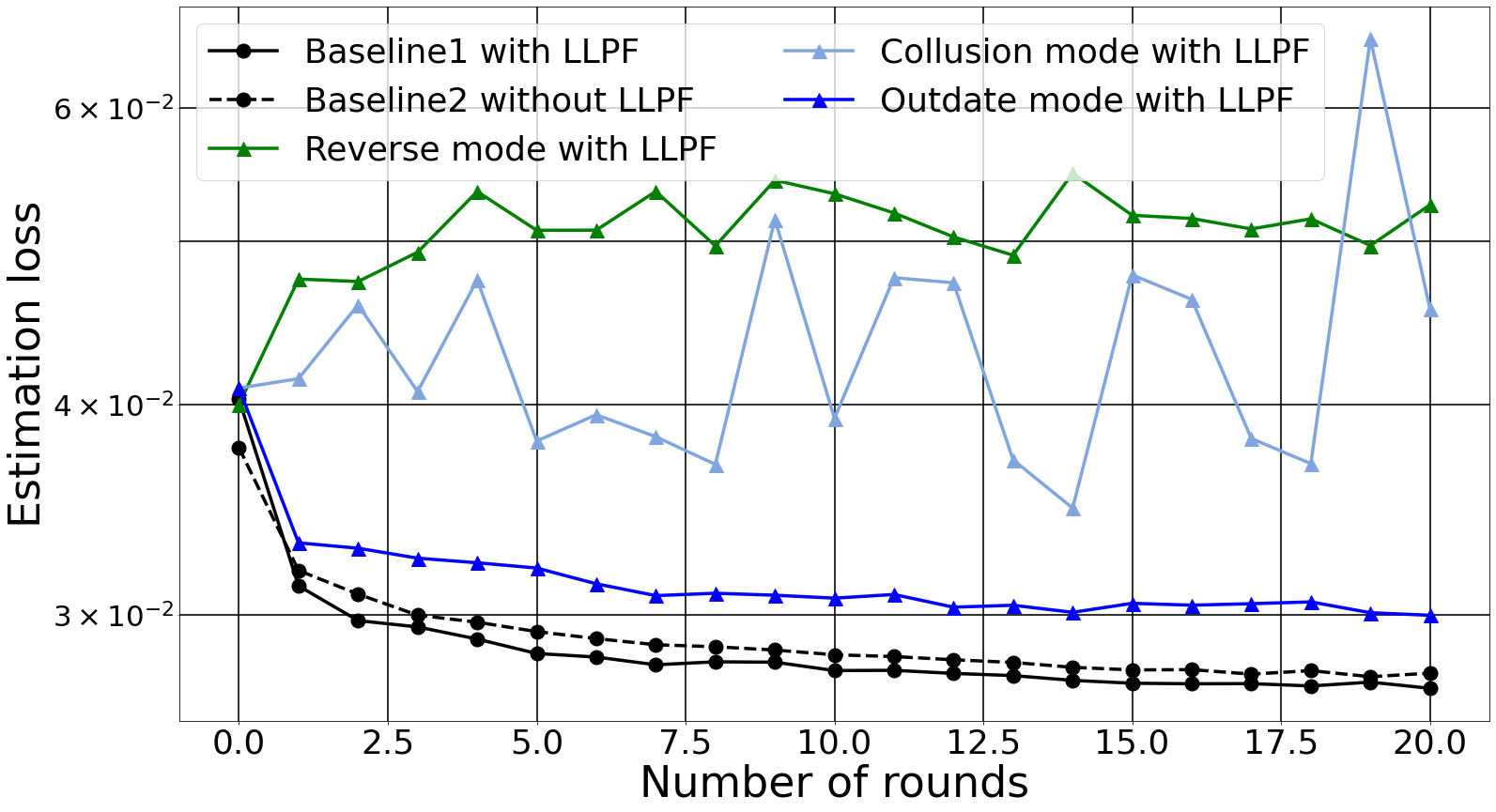
We compared the simulation results with two baselines, obtained by excluding of the authentic data. The results depicted in Fig.4 indicate that employing LLPF leads to a slight improvement in convergence performance. When comparing the reverse mode and collusion mode in Fig. 4(a), the attack performance of collusion mode exhibits high fluctuations. This observation aligns with our analysis in Sec.III, confirming that the performance of collusion attacks strongly depends on the variety of data.
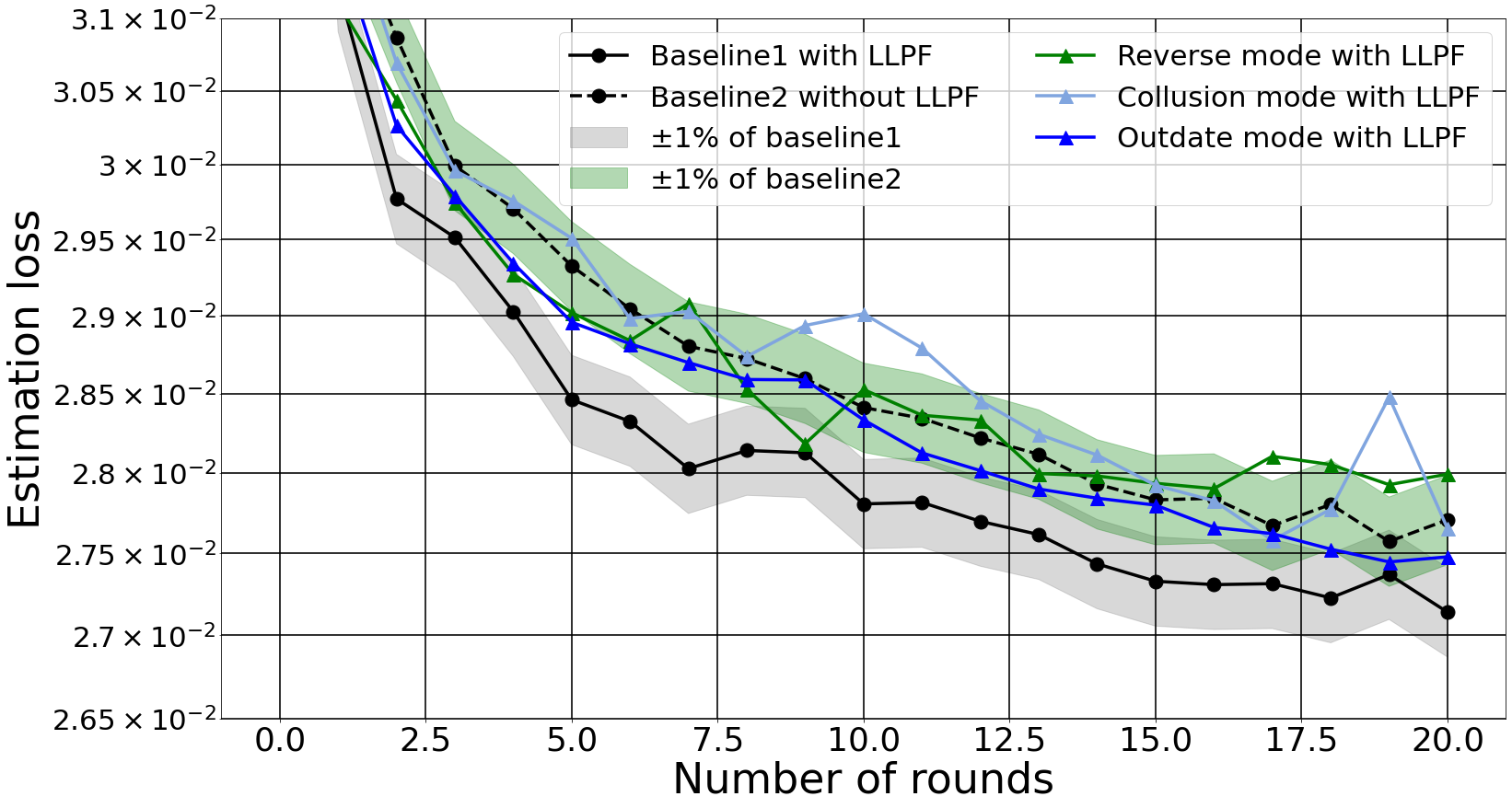
In Fig. 4(b), LLPF exhibited robust performance against all attack modes, with performance levels roughly converging to of baseline2. However, considering a certain level of miss-detection is inevitable, this prevents the convergence performance with LLPF from reaching the level of baseline1. In summary, LLPF effectively mitigate widely launched attacks as well as improve the overall performance.
VI Conclusion and outlook
This work has demonstrated the vulnerability of FL when applied in wireless communication, illustrated through a channel estimation scenario. Various adversarial attacks and strategies were devised to exploit this vulnerability. Subsequently, StoMedian was introduced to enhance resilience during the aggregation process, along with LLPF tailored for incremental training for channel estimation. Both StoMedian and LLPF have been validated through simulation.
However, the performance of the mentioned methods may be impacted when the cached data exhibit highly non-identical distributions, a factor not addressed in our paper. Particularly for LLPF, in scenarios with non-identical or highly varied data, it may filter out new features for the model to learn. To address this, a soft determination process based on the cumulative trustworthiness of MUs, as exemplified in [20], could be applied. By integrating the current determination with the MU’s historical behaviors, a smart determination process could further enhance model convergence.
Acknowledgment
This work is supported partly by the German Federal Ministry of Education and Research within the project Open6GHub (16KISK003K/16KISK004), partly by the European Commission within the Horizon Europe project Hexa-X-II (101095759). B. Han (bin.han@rptu.de) is the corresponding author.
References
- [1] N. H. Tran, W. Bao, A. Zomaya et al., “Federated learning over wireless networks: Optimization model design and analysis,” in IEEE INFOCOM 2019 - IEEE Conference on Computer Communications, 2019, pp. 1387–1395.
- [2] S. Niknam, H. S. Dhillon, and J. H. Reed, “Federated learning for wireless communications: Motivation, opportunities, and challenges,” IEEE Communications Magazine, vol. 58, no. 6, pp. 46–51, 2020.
- [3] S. M. Sheikholeslami, A. Rasti-Meymandi, S. J. Seyed-Mohammadi et al., “Communication-efficient federated learning for hybrid vlc/rf indoor systems,” IEEE Access, vol. 10, pp. 126 479–126 493, 2022.
- [4] M. M. Wadu, S. Samarakoon, and M. Bennis, “Federated learning under channel uncertainty: Joint client scheduling and resource allocation,” in 2020 IEEE Wireless Communications and Networking Conference (WCNC), 2020, pp. 1–6.
- [5] A. M. Elbir and S. Coleri, “Federated learning for hybrid beamforming in mm-wave massive MIMO,” IEEE Communications Letters, vol. 24, no. 12, pp. 2795–2799, 2020.
- [6] S. Elbir, Ahmet M.and Coleri, “Federated learning for channel estimation in conventional and ris-assisted massive MIMO,” IEEE Transactions on Wireless Communications, vol. 21, no. 6, pp. 4255–4268, 2022.
- [7] S. Shahabodini, M. Mansoori, J. Abouei et al., “Recurrent neural network and federated learning based channel estimation approach in mmwave massive MIMO systems,” Transactions on Emerging Telecommunications Technologies, vol. 35, 12 2023.
- [8] Y.-S. Jeon, M. Mohammadi Amiri, and N. Lee, “Communication-efficient federated learning over MIMO multiple access channels,” IEEE Transactions on Communications, vol. 70, no. 10, pp. 6547–6562, 2022.
- [9] M. M. Amiri and D. Gündüz, “Federated learning over wireless fading channels,” IEEE Transactions on Wireless Communications, vol. 19, no. 5, pp. 3546–3557, 2020.
- [10] M. S. H. Abad, E. Ozfatura, D. GUndUz et al., “Hierarchical federated learning across heterogeneous cellular networks,” in ICASSP 2020 - 2020 IEEE International Conference on Acoustics, Speech and Signal Processing (ICASSP), 2020, pp. 8866–8870.
- [11] W. Hou, J. Sun, G. Gui et al., “Federated learning for dl-csi prediction in fdd massive MIMO systems,” IEEE Wireless Communications Letters, vol. 10, no. 8, pp. 1810–1814, 2021.
- [12] J.-P. Hong, S. Park, and W. Choi, “Base station dataset-assisted broadband over-the-air aggregation for communication-efficient federated learning,” IEEE Transactions on Wireless Communications, vol. 22, no. 11, pp. 7259–7272, 2023.
- [13] Y. Cao, S. Maghsudi, T. Ohtsuki et al., “Mobility-aware routing and caching in small cell networks using federated learning,” IEEE Transactions on Communications, pp. 1–1, 2023.
- [14] E. M. Campos, A. G. Vidal, J. L. H. Ramos et al., “FedRDF: A robust and dynamic aggregation function against poisoning attacks in federated learning,” 2024, preprint available at arXiv:2402.10082.
- [15] V. Rey, P. M. Sánchez Sánchez, A. Huertas Celdrán et al., “Federated learning for malware detection in IoT devices,” Computer Networks, vol. 204, p. 108693, 2022.
- [16] L. Cao, H. Chen, X. Fan et al., “Bayesian federated learning: A survey,” in IJCAI-23, 8 2023, pp. 7233–7242, survey Track.
- [17] H.-Y. Chen and W.-L. Chao, “FedBE: Making bayesian model ensemble applicable to federated learning,” in International Conference on Learning Representations, 2021.
- [18] B. Han and H. D. Schotten, “A secure and robust approach for distance-based mutual positioning of unmanned aerial vehicles,” 2024, to appear at IEEE WCNC 2024, preprint available at arXiv:2305.12021.
- [19] F. O. Catak, M. Kuzlu, E. Catak et al., “Defensive distillation-based adversarial attack mitigation method for channel estimation using deep learning models in next-generation wireless networks,” IEEE Access, vol. 10, pp. 98 191–98 203, 2022.
- [20] Z. Fang, B. Han, and H. D. Schotten, “A reliable and resilient framework for multi-uav mutual localization,” in 2023 IEEE 98th Vehicular Technology Conference (VTC2023-Fall), 2023, pp. 1–7.