Eternal Universes

Abstract

We consider the possibility of a past and future eternal universe, constructing geodesically complete inflating, loitering, and bouncing spacetimes. We identify the constraints energy conditions in General Relativity place on the building of eternal cosmological models. Inflationary and bouncing behavior are shown to be essential ingredients in all significant examples. Non-trivial complete spacetimes are shown to violate the null energy condition (NEC) for at least some amount of time, although, some obey the average null energy condition. Ignoring the intractable subtleties introduced by quantum considerations, such as rare tunneling events and Boltzmann brains, we demonstrate that these universes need not have had a beginning or an end.

I Introduction

Contemplating the vastness of the universe is an innate aspect of human curiosity. We are not only drawn to ponder the physical expanse of space and whether the universe stretches infinitely but also the expanse of the dimension of time. Could the universe have endured for an eternity into the past and what will be its ultimate fate? In this paper we explore these questions from a conservative viewpoint using simple arguments from General Relativity (GR) and a field theoretic treatment of matter and energy. Our goal is to be as rigorous as possible using our known, tested laws of physics. We operate within a framework of metrical geometry and apply the results to classical Einstein gravity. Within this context we provide examples of geodesically complete past and future eternal cosmological solutions.

Whether or not the universe had a beginning is a question that naturally arises within our most successful theory of the early universe, the theory of inflation Guth (1981); Linde (1982); Albrecht and Steinhardt (1982). Soon after the theory’s inception it became clear that once inflation started, it would never stop. While early-time inflation has ceased in our observable universe, allowing galaxies and structures to form, it continues indefinitely in other parts of the universe, and hence, inflation is eternal into the future. Specifically, quantum fluctuations in the field responsible for the accelerated expansion can cause the field to remain in its high-energy state, sustaining inflation in those regions indefinitely 198 (1983); Vilenkin (1983); Linde (1986); Guth (2007). In a Letter by Borde, Guth and Vilenkin (BGV) Borde et al. (2003), it was subsequently argued that inflation cannot likewise be eternal into the past; although, we have countered this belief Easson and Lesnefsky (2024); Lesnefsky et al. (2023a) and present further evidence that inflation can, in fact, be eternal into the past in the current work. Acknowledging the possibility of a past eternal universe opens entirely new avenues of research. We show there are multiple ways that the universe can sustain itself within classical General Relativity for an eternity, albeit at the expense of violation of certain energy conditions.

Three broad categories of an eternal universe are suggested. Our examples are admittedly toy models; however, given the wide variety we expect our findings to be quite general and applicable to many solutions of interest. In particular, we will construct eternal inflationary, loitering, and bouncing cosmologies. In each case we will provide a rigorous proof of full geodesic completeness. Existing proposed no-go theorems are circumvented or obviated as discussed in detail in an accompanying Letter Easson and Lesnefsky (2024). We show that all (non-trivial) models that are eternal geodesically complete necessarily involve a phase of accelerated expansion (or inflationary phase) for at least some amount of time and generically include a bouncing phase in accordance with our reported definitions.

The models we present violate the traditional energy conditions, a property we will conjecture is necessary in GR for geodesic completeness.  In some instances violations of the null energy condition (NEC) can be limited to an arbitrarily short amount of time $\Delta t$, and confined to the primordial past.  Models presented here having such behavior are capable of satisfying the average null energy condition (ANEC).

In several known circumstances, energy condition violations can be relatively benign. For example, a simple time-independent cosmological constant $\Lambda$ violates the SEC if $\Lambda>0$ and the WEC and DEC for $\Lambda<0$. The NEC is the only energy condition which remains valid in the presence of $\Lambda$. Non-minimally coupled scalar fields are capable of violating all of the traditional energy conditions Barcelo and Visser (2002); Chatterjee et al. (2013). Indeed, all classical energy conditions are manifestly violated by quantum effects both experimentally and theoretically Epstein et al. (1965), (e.g., the Casimir Effect Casimir (1948)). Even the NEC is violated ubiquitously in particle physics, for example, during the Hawking radiation process local energy density can become negative from the perspective of certain observers and interpreted as violation of NEC. In theories outside of pure GR, which can mix gravitational and matter degrees of freedom in a non-trivial way through non-minimal and higher-derivative terms or couplings, it becomes difficult to adequately define analogues of energy conditions in the first place (see e.g., Chatterjee et al. (2013)).

As is well known, violation of energy conditions are necessary in order to avoid singularities. Within classical GR non-trivial flat cosmological solutions which avoid singularities must violate energy conditions to circumvent the singularity theorems Penrose (1965); Hawking (1966a, b, 1967); Hawking and Penrose (1970); Hawking and Ellis (2023). On occasion, the NEC can be violated in a stable way Dubovsky et al. (2006); Nicolis et al. (2010); Kobayashi et al. (2010); Deffayet et al. (2010); Sawicki and Vikman (2013); Rubakov (2014); Cai et al. (2017a); Creminelli et al. (2016); Cai et al. (2017b); Easson and Manton (2019); Alexandre and Polonyi (2021); Alexandre and Backhouse (2023), sometimes allowing for well-behaved cosmological bouncing solutions Easson et al. (2011); Cai et al. (2012); Easson and Vikman (2016); Ijjas and Steinhardt (2016, 2017); Cai and Piao (2017); Alexandre and Pla (2023).

Currently known consistent quantum field theories in flat spacetime obey the averaged null energy condition (ANEC), for a complete achronal null geodesic (those that do not contain any points connected by a timelike curve) Wald and Yurtsever (1991); Graham and Olum (2007); Hartman et al. (2017). Effectively, the ANEC condition quantifies the degree of violation of the null energy condition. The condition is expected to rule out closed timelike curves, time machines and wormholes connecting different asymptotically flat regions Morris et al. (1988); Friedman et al. (1993). Matter violating the ANEC can be used to violate the second law of thermodynamics Wall (2010).

The ANEC may be stated

$$\int_{\gamma}T_{\mu\nu}k^{\mu}k^{\nu}d\lambda\geq 0\,,$$ (1.1)

where the integral is over a null geodesic $\gamma$ with tangent vector $k^{\mu}=dx^{\mu}/d\lambda$, and $\lambda$ is an affine parameter with respect to which the tangent vector to the geodesic is defined. In GR, it is frequently convenient to replace $T_{\mu\nu}$ in Eq. 1.1 by the Ricci tensor $R_{\mu\nu}$, simply using the Einstein field equations and the definition of a null vector. The ANEC has been shown to hold even in the case of arbitrary Casimir systems as long as the geodesic does not intersect or asymptotically approach the plates Graham and Olum (2005); Fewster et al. (2007). If the null geodesic is not assumed to be achronal, the ANEC may be violated by a quantum scalar field in a spacetime compactified in one spatial dimension or in the spacetime around a Schwarzschild black hole Visser (1996). As we shall see some of the eternal models we construct are capable of satisfying the ANEC.

Given the many nuances involved with respect to energy condition violation and stability, it can be difficult to pass definitive judgment on the validity of solutions which experience such violations. In this work we refrain from making such criticisms as more rigorous analysis of specific situations is needed; however, it is clear that at least some violations do not lead to pathologies and ultimately singularity formation is arguably a worst-case malady plaguing a given physical solution. Yet many physically relevant and useful solutions in GR contain such singularities, even at the level of the vacuum solutions, for example, the singular Schwarzschild and Kerr black hole solutions.

After assembling a diverse grouping of possible eternal universe models, our analysis demonstrates that there are no known obstructions indicating the universe must have had a “first moment”. In the context of the inflationary universe paradigm, this translates into the statement that inflation need not have had a beginning.

This is the companion paper to our Letter Easson and Lesnefsky (2024). A few of the Theorems and Corollaries we discuss were presented without proof in our earlier work Lesnefsky et al. (2023b); Easson and Lesnefsky (2024). The proofs are revealed presently.

An outline of this paper is as follows. In section II, we prove a theorem which definitively provides the criteria for geodesic completeness of generalized Friedmann-Robertson-Walker (GFRW) spacetimes. In section III, we discuss the definition of inflation and bouncing cosmologies and provide an example of an eternally inflating universe which is eternal and geodesically complete both into the past and future. In section IV, we provide examples of eternal bouncing cosmologies which are geodesically complete both into the past and future. In section V, we provide examples of loitering (and quasi-loitering) models which are eternal and geodesically complete both into the past and future. Finally, in section VI, we present a discussion and our conclusions. We provide appendices to discuss the energy conditions in General Relativity with respect to cosmology, to provide proof details and to define Generalized Friedmann-Robertson-Walker (GFRW) spacetimes.

II Geodesic Completeness

We begin with a rigorous discussion of what it means to be geodesically complete within the context of GFRW spacetimes (which include the familiar FRW spacetimes). Stated formally, a GFRW spacetime is the warped product - see Bishop and O’Neill (1969); O’Neill (1983) - given by $\mathbb{R}^{1}_{1}\times_{a}\Sigma$ where $\left(\Sigma,g_{\Sigma}\right)$ is a complete Riemannian manifold and scale factor $a\in\mathcal{C}^{\infty}\left(\mathbb{R}^{1}_{1}\right)$ which is smooth and $a>0$. To fully explore the geodesic completeness of a spacetime manifold $\mathcal{M}$, we must explore maximal geodesics: consider a maximal geodesic $\gamma:I\to\mathcal{M}$, where $I$ is an open interval of $\mathbb{R}$, and, because geodesics are usually parameterized with constant speed, it is uniquely defined up to transversality. A manifold is geodesically complete if every geodesic $\gamma$, $I=(-\infty,\infty)$, is defined for all time (see e.g. O’Neill (1983), Prop. 7.38).

We now construct a theorem quantifying the criteria for geodesic completeness of a GFRW spacetime having scale factor $a$. A geodesic $\gamma\left(\lambda\right)=\left(t\left(\lambda\right),\beta\left(\lambda\right)\right)$ in a warped product spacetime of $\mathbb{R}^{1}_{1}\times_{a}\Sigma$ obeys

$$\nabla_{\frac{\partial}{\partial t}}\frac{\partial}{\partial t}=g_{\Sigma}\left(\beta^{\prime},\beta^{\prime}\right)\left(a\left(t\left(\lambda\right)\right)\right)\left(\mathrm{grad}_{-dt^{2}}a\right)\,,$$ (2.2)

in $\mathbb{R}^{1}_{1}$ and

$$\nabla_{\beta^{\prime}}\beta^{\prime}=-\frac{2}{a\left(t\left(\lambda\right)\right)}\left(\beta^{\prime}\right)\frac{d}{d\lambda}\left[a\left(t\left(\lambda\right)\right)\right]\,,$$ (2.3)

in Riemannian manifold spacelike leaf $\left(\Sigma,g_{\Sigma}\right)$ where the geodesic equation $\nabla_{\gamma^{\prime}}\gamma^{\prime}=0$ has been projected down into the respective spaces $\mathbb{R}^{1}_{1}$ and $\left(\Sigma,g_{\Sigma}\right)$. The coupled ordinary differential equations (ODE) can be solved exactly yielding an integral solution as a functional of $a$. With appropriately selected initial conditions, one finds

$$\lambda\left(t\right)=\int^{t}\frac{a\left(\zeta\right)}{\sqrt{a^{2}\left(\zeta\right)+1}}d\zeta\,,$$ (2.4)

as an integral solution to Eqs. 2.2 and 2.3 for timelike initial conditions and

$$\lambda\left(t\right)=\int^{t}a\left(\zeta\right)d\zeta\,,$$ (2.5)

for null initial conditions. To solve the ODE we invert $\lambda\left(t\right)$, instead of using $t\left(\lambda\right)$; which is auspicious, because if Eqs. 2.4 and 2.5 diverge then the domain of $\gamma$ is cofinite and the geodesic ray has domain $\left[0,\infty\right)$ and is complete.

Eq. 2.3 defines a pregeodesic and thus has a geodesic reparameterization. Appropriately reparameterizing, there is a geodesic in $\Sigma$ which has $\beta$ as its image: thus, if $\left(\Sigma,g_{\Sigma}\right)$ is complete as a Riemannian manifold, then the limiting factor to geodesic completeness is Eq. 2.2 with solutions of Eqs. 2.2 and 2.3. The assumption of “generality” in a GFRW is the least restrictive logical assumption needed to have Eqs. 2.2 and 2.3 characterize geodesic completeness of GFRWs. Hence, the criteria for geodesic completeness of a GFRW spacetime is given by Thm. 2 of Lesnefsky et al. (2023b) (which builds on previous work Sanchez (1998)). The theorem states:

Theorem 1.

Let $\mathcal{M}=\mathbb{R}^{1}_{1}\times_{a}\Sigma$ be a GFRW spacetime.

1. The spacetime $\mathcal{M}$ is future timelike complete iff $\int_{t_{0}}^{\infty}\frac{a\left(\zeta\right)d\zeta}{\sqrt{\left(a\left(\zeta\right)\right)^{2}+1}}$ diverges for all $t_{0}\in\mathbb{R}$.

2. The spacetime $\mathcal{M}$ is future null complete iff $\int_{t_{0}}^{\infty}a\left(\zeta\right)d\zeta$ diverges for all $t_{0}\in\mathbb{R}$.

3. The spacetime $\mathcal{M}$ is future spacelike complete iff $\mathcal{M}$ is future null complete and $a<\infty$.

4. The GFRW is past timelike / null / spacelike complete if, for items 1-3 above, upon reversing the limits of integration from $\int_{t_{0}}^{\infty}$ to $\int_{-\infty}^{t_{0}}$ the word “future” is replaced by “past”.

5. The spacetime $\mathcal{M}$ is geodesically complete iff it is both future and past timelike, null, and spacelike geodesically complete.

Proof.

The definition of a geodesically complete manifold $\mathcal{M}$ is a manifold where all geodesics are defined for all $\mathbb{R}$. Given the structure of $\mathbb{R}^{1}_{1}\times_{a}\Sigma$ the geodesic equation projections of Eqs. 2.2,2.3 reduce to an integral over $\mathbb{R}^{1}_{1}$. One must discriminate the space $\mathbb{R}^{1}_{1}\times_{\exp t}\Sigma$, appropriate for the cosmological flat slicing of de Sitter space, which is known to be past geodesically incomplete (see e.g.O’Neill (1983), Example 7.41). The integration $\int_{\mathbb{R}^{1}_{1}}\frac{d\zeta a}{\sqrt{a^{2}+1}}$ diverges, yet the model is past incomplete, in particular, the mass density from the (complete) future divergence obfuscates the mass density of the (incomplete) past convergence.

Using future and / or past directed maximal geodesic rays, for example $\gamma:\left[0,b\right)\rightarrow\mathcal{M}$, completeness requires for all initial points $p\in\mathcal{M}$, the endpoint $b\rightarrow\infty$. In the case of a geodesic $\gamma\left(\lambda\right)=t\left(\lambda\right)\oplus x^{k}\left(\lambda\right)$ of $\mathbb{R}^{1}_{1}\times_{a}\Sigma$, integral divergence is required for all future directed geodesic rays

$$\int_{t_{0}}^{\infty}\frac{d\zeta a\left(\zeta\right)}{\sqrt{w_{0}a^{2}\left(\zeta\right)+1}}\,,$$ (2.6)

and past directed geodesic rays

$$\int_{-\infty}^{t_{0}}\frac{d\zeta a\left(\zeta\right)}{\sqrt{w_{0}a^{2}\left(\zeta\right)+1}}\,,$$ (2.7)

because in both of these cases the integral computes the range of the affine parameter $\lambda\left(t\right)$ and if $\lambda\left(t\right)$ diverges, no finite $b$ exists for domain $\left[0,b\right)$. Independent of causal character this proves item (4). The integral constant $w_{0}$ encapsulates causal character with $w_{0}\in\left\{+1,0,-1\right\}$ for timelike, null, and spacelike, respectively. Items (1), (2) trivially follow from evaluation of $w_{0}=+1$ and $w_{0}=0$.

The proof of Item (3) pertaining to spacelike completeness is less straightforward and not relevant for our primary discussion and hence, relegated to Appendix B.

∎

II.1 Singularities

In our effort to build geodesically complete spacetimes, we pause to further consider the catastrophes which can prevent completeness. Perhaps the most common object leading to incomplete geodesics is the curvature singularity, where a curvature invariant such as the Kretschmann scalar $K=R_{\mu\nu\kappa\sigma}R^{\mu\nu\kappa\sigma}$, built from the Riemann tensor, diverges at a particular place, or time. Infamous examples of curvature singularities lie at the center of the Schwarzschild black hole or at the cosmological Big-Bang. Generally, curvature singularities occur in regions of spacetime with high curvature, where quantum gravity effects are expected to be significant. In some of our models, it is possible to arrange parameter values so that the energy and curvature scales remain significantly lower than the Planck regime for the entire cosmological evolution, thereby avoiding conditions where quantum gravity is necessary. Consequently, quantum gravity might not play a critical role in the development of an eternal universe.

In order to avoid cosmological singularities it is necessary to violate classical energy conditions in GR. These violations are anticipated to manifest close to the would-be singularity formation points and, occasionally, can be confined to an arbitrarily brief period. Arguably these energy condition violations are a lesser inconvenience when weighed against the formation of singularities, at which point all established physical laws cease to apply.

Of course, it is possible for a spacetime to be geodesically incomplete even without encountering a curvature singularity. The most renowned example is the incompleteness encountered in the flat cosmological slicing of de Sitter space, where an observer following a geodesic into the past encounters a boundary in finite proper time (for a recent discussion see Kinney et al. (2023)).

Yet another, arguably less common malady is a big rip, Caldwell et al. (2003), a catastrophic “phantom” force that eventually tears the universe apart. This type of cataclysm can occur in models which are dominated by NEC violating matter for a sufficiently long period of time. As a demonstration we construct the following example. We adopt a perfect-fluid description of matter with equation of state (EOS)

$$p=w\rho\,,$$ (2.8)

where $w$ is the equation of state parameter relating the pressure $p$ to the energy density $\rho$ of the fluid. We now force this fluid to violate the NEC for all time, thus also violating the ANEC. From the NEC condition $\rho+p=\rho(1+w)\geq 0$ (see Append. A), the fluid will have EOS parameter $w<-1$ in order to violate NEC. We take a flat $k=0$ FRW metric, and since $\dot{H}\propto-\rho(1+w)$, we find NEC violation implies $\dot{H}>0$ for $\rho>0$. We now take $\dot{H}=\ddot{a}/a-(\dot{a}/a)^{2}=2/\beta^{2}$, for a positive constant $\beta$, and integrate to get

$$a(t)=a_{0}\,\exp{\left[\frac{t}{\alpha}+\left(\frac{t}{\beta}\right)^{2}\right]}\,.$$ (2.9)

This spacetime is eternally super-inflating with $\dot{H}>0$ and an energy density which grows without bound from $t=0$ to $t\rightarrow\infty$ and violates the NEC for all time. Such a universe cannot sustain itself as it will inevitably encounter a big rip. The Ricci scalar, for example, is given by

$$R=12\left(\frac{1}{\beta^{2}}+\frac{(\beta^{2}+2\alpha t)^{2}}{\alpha^{2}\beta^{4}}\right)\,,$$ (2.10)

which diverges in a singular fashion as $t\rightarrow\infty$. The Kretschmann scalar $K=R_{\mu\nu\kappa\sigma}R^{\mu\nu\kappa\sigma}\propto t^{4}$, likewise diverges at $t\rightarrow\infty$. Geometrically, the geodesically connected domains of any point become arbitrarily small as the scale factor and curvatures become arbitrarily large. Eventually, the geodesically connected domain becomes smaller than a Planck volume, although the affine parameter of a geodesic is still defined. Hence, in general, it is difficult to construct a physically reasonable eternal cosmological model with such extended period of NEC violation.

To summarize, a geodesic $\gamma:I\to\mathcal{M}$ may fail be be complete – where $I\neq\mathbb{R}$ – for any of the above reasons, including a curve encountering a curvature singularity at a (topological) limit point, a causal curve encountering a spacelike boundary $\partial\mathcal{M}$ at a limit point, or light cones on a geodesic “tipping over” where said curve changes causal character. 

II.2 Inflationary and bouncing cosmologies

In preparation for our eternal universe constructions and to further hone our discussion, we offer the following definitions.

Definition 1.

Let $\left(\mathcal{M},g\right)$ be an $n$ dimensional spacetime which admits a connected open neighborhood $U\subset\mathcal{M}$ which is isometric to $\left(b,c\right)\times_{a}V$ as a warped product open submanifold, where $\left(b,c\right)$ is a timelike codimension $n-1$ embedded submanifold, $V$ is a connected spacelike codimension 1 embedded submanifold and no assumptions are made concerning $a(t)$ except that it is a well defined function between sets. The spacetime $\left(\mathcal{M},g\right)$ is an inflationary spacetime if there exists some $t_{0}\in\left(b,c\right)$ such that (assuming that it exists and is well defined), $\ddot{a}\left(t_{0}\right)>0$ where derivatives of the scale factor are taken with respect to the timelike $\left(b,c\right)$ coordinate and the sign of $\ddot{a}$ is given with respect to the time orientation of $\mathcal{M}$.

Note, in the above definition of inflation we make no assumptions about the continuity of the scale factor $a$ or its derivatives. Furthermore, this definition includes arbitrarily short periods of accelerated expansion as inflationary. We are aware some readers will find this objectionable; however, if one wishes to distinguish the terms “short accelerated expansion” from “inflation”, one is obliged to set an arbitrary scale for the duration of the acceleration. While GUT-scale inflation naturally requires at least 60 e-foldings of accelerated expansion to solve the flatness and horizon problems, low-energy (e.g., TeV-scale) inflation does the job with far fewer. It is only a few e-foldings of accelerated expansion that are actually probed in the cosmic microwave background radiation (CMB). In the present context of an eternal universe the difference between a few e-folding, and 60 e-foldings is entirely insignificant. For these reasons we find it unnecessary to reserve the term inflation to designate significant prolonged expansion and use the term interchangeably with accelerated expansion as is appropriate considering Defn. 1. This is the definition of “inflation” from Lesnefsky et al. (2023b), which we have reproduced here to align with our present notation.

We further suggest the following definition for a “bouncing” spacetime:

Definition 2.

Let $\left(\mathcal{M},g\right)$ be an $n$ dimensional spacetime which admits a connected open neighborhood $U\subset\mathcal{M}$ which is isometric to $\left(b,c\right)\times_{a}V$ as a warped product open submanifold, where $\left(b,c\right)$ is a timelike codimension $n-1$ embedded submanifold, $V$ is a connected spacelike codimension 1 embedded submanifold and no assumptions are made concerning $a(t)$ except that it is a well defined non-constant function between sets. The spacetime $\left(\mathcal{M},g\right)$ is a bouncing spacetime if there exists some $t_{0}\in\left(b,c\right)$ such that (assuming that it exists and is well defined), $\dot{a}(t_{0})=0$, where derivatives of the scale factor are taken with respect to the timelike $\left(b,c\right)$ coordinate and the sign of $\dot{a}$ is given with respect to the time orientation of $\mathcal{M}$.

As we shall discover, in some cases it is advantageous to discuss a “bounce at infinity”. Considering that the point at infinity is strictly not an element of $\mathbb{R}$, we suggest:

Definition 3.

A neighborhood $\left(b,c\right)\times_{a}V\subset\left(\mathcal{M},g\right)$ is an open submanifold which is isometric to a GFRW $\left(b,c\right)\times_{a}\Sigma\subset\mathcal{M}$ is said to admit a bounce at positive infinity $+\infty$ if $c\rightarrow+\infty$ is unbounded above and there exists a divergent cofinite sequence $\left\{t_{\ell}\right\}_{\ell=1}^{\infty}\rightarrow+\infty$ with $t_{k}>t_{\ell}$ for $k>\ell$ where $\left\{\dot{a}\left(t_{\ell}\right)\right\}_{\ell=1}^{\infty}\rightarrow 0$ constitutes a convergent Cauchy sequence.

A neighborhood $\left(b,c\right)\times_{a}V\subset\left(\mathcal{M},g\right)\subset\mathcal{M}$ is an open submanifold which is isometric to a GFRW which admits a bounce at negative infinity $-\infty$ if $b\rightarrow-\infty$ is unbounded below and there exists a divergent cofinite sequence $\left\{t_{\ell}\right\}_{\ell=1}^{\infty}\rightarrow-\infty$ with $t_{k}<t_{\ell}$ for $k>\ell$ where $\left\{\dot{a}\left(t_{\ell}\right)\right\}_{\ell=1}^{\infty}\rightarrow 0$ constitutes a convergent Cauchy sequence.

A neighborhood $\left(b,c\right)\times_{a}V\subset\left(\mathcal{M},g\right)\subset\mathcal{M}$ is an open submanifold which is isometric to a GFRW which admits a bounce at infinity if it admits a bounce at positive infinity and / or a bounce at negative infinity.

In this definition we require the Hubble parameter $H=\dot{a}/a$ be non-zero for some time on the interval $\left(b,c\right)$ to exclude referring to pure Minkowski as a bouncing spacetime. (One may likewise exclude Minkowski spacetime by requiring there be no timelike killing vector for $\left(\mathcal{M},g\right)$.) In the following we shall casually refer to a spacetime as a bouncing spacetime if it incorporates either a bounce at finite $t$, or a bounce at infinity in accordance with the above definitions.

We are now in a position to build diverse examples of geodescially complete spacetimes.

III Eternal inflating universe

Our first example of an eternal universe was introduced in Lesnefsky et al. (2023b), and analyzed in detail in Easson and Lesnefsky (2024):

$$a(t)=a_{0}\,e^{\frac{2t}{\alpha}}+c\,,$$ (3.11)

for real constants $a_{0}>0$, $\alpha$, and $c>0$.

Application of Thm. 1, finds that the scale factor (3.11) with $c>0$, defines a geodesically complete spacetime for all (real) values of the parameter $\alpha$. The theorem integrals are explicitly calculated in Easson and Lesnefsky (2024). The Hubble parameter $H=\dot{a}/a$ is given by:

$$H=\frac{2a_{0}e^{\frac{2t}{\alpha}}}{(c+a_{0}e^{\frac{2t}{\alpha}})\alpha}\,.$$ (3.12)

This is an example of an eternally inflating spacetime in accordance with Defn. 1:

$$\frac{\ddot{a}}{a}=4\alpha^{-2}\left(1-\frac{c}{c+a_{0}e^{\frac{2t}{\alpha}}}\right)\,.$$ (3.13)

The acceleration is positive for all $t\in(-\infty,\infty)$ for all non-zero values of $\alpha$ with $c>0$. For $\alpha>0$, the universe is expanding and inflating for all $t$. For $\alpha<0$ the universe is contracting yet inflating ($\ddot{a}>0$) for all time, approaching zero acceleration as $t\rightarrow\infty$.

The cosmological evolution is depicted in Fig. 1. Shown are the scale factor $a(t)$, Hubble parameter $H$ (amplified by a factor of 100) and co-moving Hubble radius $1/aH$. When the co-moving Hubble radius is decreasing the spacetime is inflating–in this case it is decreasing for all $t$.

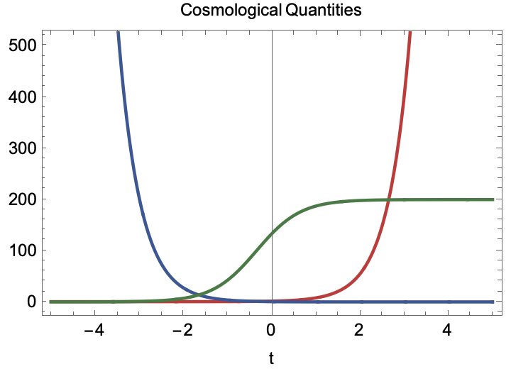
Figure 1: Evolutionary behavior for (3.11). The scale factor is plotted in red. The Hubble parameter (green). The co-moving Hubble radius (blue). Model parameters: $a_{0}=c=1/2$, $\alpha=1$.

The spacetime is geodesically complete, eternal and inflating, and provides a simple counterexample to the statement that inflationary models must be past incomplete, regardless of energy condition considerations (see, Borde et al. (2003)). It is only one example of an infinite number of models with such behavior as we shall see in the proceeding discussion.  For $\alpha>0$, the universe approaches Minkowski spacetime as $t\rightarrow-\infty$; however, an observer travelling along a past-directed geodesic will experience an infinite proper time to reach the non-accelerating Minkowski space at the point $t=-\infty$ and hence, the model is an eternal inflating spacetime. As we shall see, another eternal inflating example having $\ddot{a}>0$ $\forall\,t\in\left(-\infty,\infty\right)$, is given by Eq. 4.24.

One may identify the absence of curvature singularities from the curvature invariants, as shown in Fig. 2. We plot the Ricci scalar $R$ and the Kretchmann scalar $K=R_{\mu\nu\rho\sigma}R^{\mu\nu\rho\sigma}$ built from the Riemann tensor. Both are observed to be finite for all $t$:

$$R=\frac{24a_{0}e^{\frac{2t}{\alpha}}(c+2a_{0}e^{\frac{2t}{\alpha}})}{(c+a_{0}e^{\frac{2t}{\alpha}})^{2}\alpha^{2}}\,,\qquad K=\frac{192a_{0}^{2}e^{\frac{4t}{\alpha}}(c^{2}+2a_{0}ce^{\frac{2t}{\alpha}}+2a_{0}^{2}e^{\frac{4t}{\alpha}})}{(c+a_{0}e^{\frac{2t}{\alpha}})^{4}\alpha^{4}}\,.$$ (3.14)

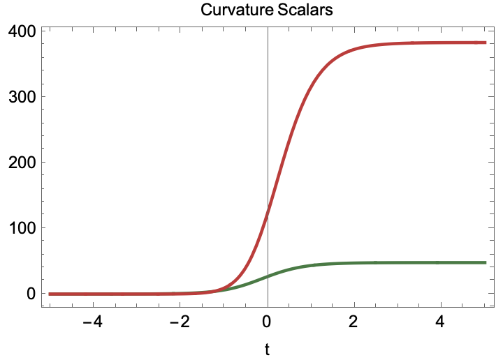
Figure 2: Curvature invariants computed from (3.11). The Ricci scalar is plotted in green and the Kretchmann scalar is plotted in red. Model parameters: $a_{0}=c=1/2$, $\alpha=1$.

We now examine the energy conditions for the model given by (3.11). Calculation of the Einstein tensor yields non-vanishing components:

$$G_{tt} = \frac{12a_{0}^{2}e^{\frac{4t}{\alpha}}}{(c+a_{0}e^{\frac{2t}{\alpha}})^{2}\alpha^{2}}\,,$$

$$G_{ii} = -\frac{4a_{0}e^{\frac{2t}{\alpha}}(2c+3a_{0}e^{\frac{2t}{\alpha}})}{\alpha^{2}}\,.$$ (3.15)

The energy density is given by $\rho=-G^{t}{}_{t}$ and the pressure is $p=G^{i}{}_{i}$. A plot depicting the energy conditions is given in Fig. 3

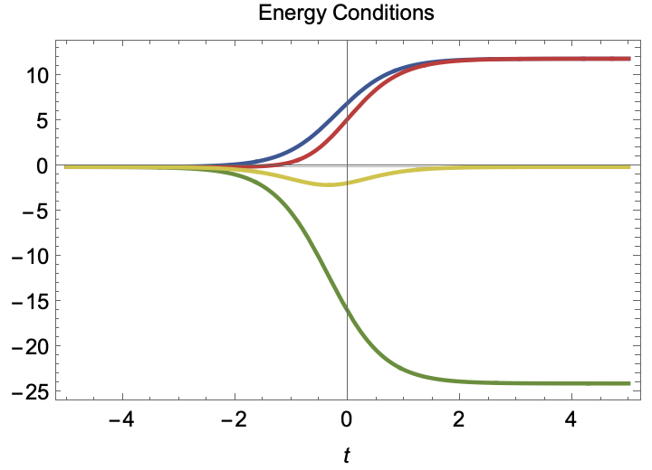
Figure 3: Energy conditions from (III). Plot of energy density $\rho$ (red), $\rho+p$ (yellow), $|p|$ (blue) and $\rho+3p$ (green). Model parameters: $a_{0}=c=1/2$, $\alpha=1$.

All of the energy conditions are violated. NEC violation is identified by the dipping of the yellow curve ($\rho+p$) below the vertical axis, both here, and in all of the proceeding energy condition plots. The NEC asymptotically approaches saturation in the early and late universe since $\rho+p=-2\operatorname{sech}^{2}{t}\rightarrow 0$ as $t\rightarrow\pm\infty$. It is easy to see the ANEC (Eq. 1.1) is also violated in this scenario. We will see that the ANEC violation is not a generic feature of eternal models. In the late universe, the SEC remains violated allowing continued acceleration, as indicated by the negativity of the green curve.

IV Eternal bouncing universe

Next we consider two bouncing models. Both models are shown to be geodesically complete, and past and future eternal, satisfying the completeness requirements of Thm. 1. The first is a transcendental function bounce and the second is a polynomial bounce. While we refer to these models as bouncing cosmologies, both models have $\ddot{a}>0$ and thus, in accordance with Defn. 1, the models are also inflationary models. We will comment further on this fact in our concluding remarks.

IV.1 Transcendental bounce

The first bouncing model we consider is given by a transcendental function scale factor:

$$a(t)=a_{0}\cosh\left(\frac{t}{\alpha}\right)\,.$$ (4.16)

The above scale factor describes a universe that contracts, bounces and then expands (similar to the familiar case of closed de Sitter).  The Hubble parameter is

$$H=\alpha^{-1}\tanh\left(\frac{t}{\alpha}\right)\,.$$ (4.17)

Remarkably, the universe is inflating for the entire evolution since:

$$\frac{\ddot{a}}{a}=\frac{1}{\alpha^{2}}\,,$$ (4.18)

and hence, this bouncing model is also an eternal inflationary model. As with our preceding example Eq. 3.11, it is possible to explicitly calculate the integrals of Thm. 1. We find for the indefinite integrals:

$$\int^{t}\frac{a\left(\zeta\right)d\zeta}{\sqrt{\left(a\left(t\right)\right)^{2}+1}}=\alpha\operatorname{arctanh}\left(\frac{a_{0}\sinh\left(\frac{t}{\alpha}\right)}{\sqrt{1+a_{0}^{2}+a_{0}^{2}\sinh\left(\frac{t}{\alpha}\right)^{2}}}\right)\,,$$ (4.19)

and

$$\int^{t}a\left(\zeta\right)d\zeta=a_{0}\alpha\sinh\left(\frac{t}{\alpha}\right)\,.$$ (4.20)

The above integrals diverge over the full set of conditions discussed in Thm. 1 for all (non-zero) values of $\alpha$; hence, the spacetime with scale factor Eq. 4.16 is geodesically complete. The cosmological evolution is depicted in Fig. 4. Shown are the scale factor $a(t)$, Hubble parameter $H$ and co-moving Hubble radius $1/aH$. As is inherent in bouncing models the co-moving Hubble radius diverges at the bounce point. When the co-moving Hubble radius is decreasing the spacetime is inflating–in this case it is decreasing for all $t$.

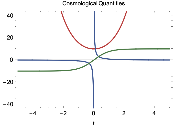
Figure 4: Evolutionary behavior for Eq. 4.16. The scale factor (red). The Hubble parameter amplified by an order of magnitude (green). The co-moving Hubble radius amplified by an order of magnitude (blue). Parameters: $a_{0}=\alpha=1$.

The Ricci scalar and Kretchsmann scalar are given by:

$$R=\frac{6\left(1+\tanh\left(\frac{t}{\alpha}\right)^{2}\right)}{\alpha^{2}}\,,\qquad K=\frac{12\left(1+\tanh\left(\frac{t}{\alpha}\right)^{4}\right)}{\alpha^{4}}\,.$$ (4.21)

We find there are no curvature singularities as inferred from the finite curvature invariants, plotted in Fig. 5

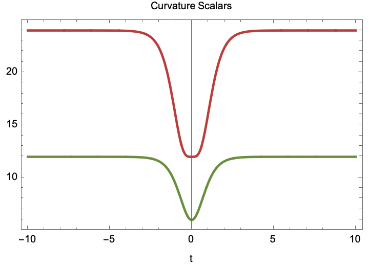
Figure 5: Curvature invariants given by Eq. 4.21. The Ricci scalar (green) and the Kretchmann scalar (red). Model parameters: $a_{0}=\alpha=1$.

Calculation of the Einstein tensor yields non-vanishing components:

$$G_{tt} = \frac{3\tanh\left(\frac{t}{\alpha}\right)^{2}}{\alpha^{2}}\,,$$

$$G_{ii} = -\frac{a_{0}^{2}(1+3\cosh\left(\frac{2t}{\alpha}\right))}{2\alpha^{2}}\,.$$ (4.22)

The energy density is given by $\rho=-G^{t}{}_{t}$ and the pressure is $p=G^{i}{}_{i}$. A plot depicting the energy conditions is given in Fig. 6

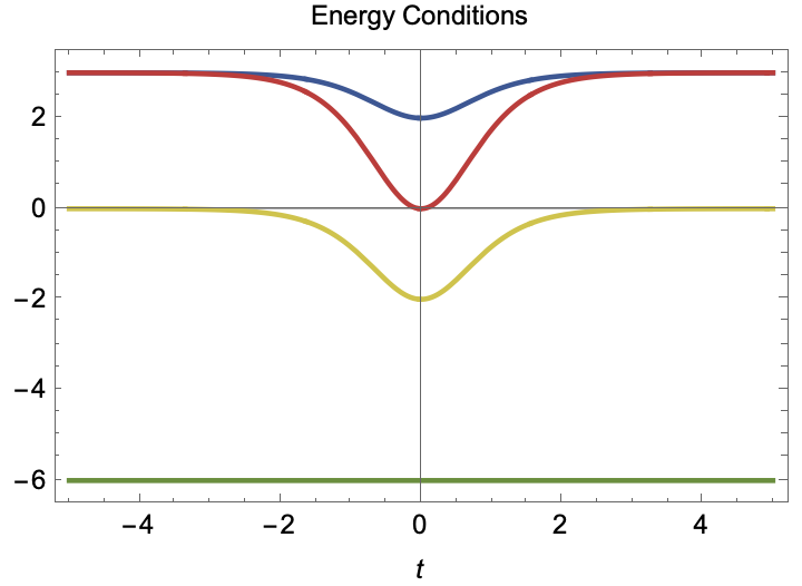
Figure 6: Energy conditions from Eq. IV.1. Plot of energy density $\rho$ (red), $\rho+p$ (yellow), $|p|$ (blue) and $\rho+3p$ (green). Model parameters: $a_{0}=\alpha=1$.

As with our previous example, all of the energy conditions including the ANEC, are violated. The SEC is violated for the entire range of the time coordinate as the model is eternally inflating, which can be seen from the eternal negativity of the green curve, and Eq. 4.18.

IV.2 Polynomial bounce

An important class of nonsingular models is given by the general polynomial function:

$$a(t)=a_{n}t^{n}+a_{n-1}t^{n-1}+\ldots+a_{2}t^{2}+a_{1}t+a_{0}\,.$$ (4.23)

In order to avoid having $a$ become negative somewhere on the interval $t\in(-\infty,\infty)$, our polynomial must have even degree and $a_{n}>0$. With respect to Thm. 1, we derive the following with respect to a scale factor $p(t)$:

Corollary 2.

Let $p\left(t\right)\in\mathbb{R}\left[t\right]$ be a polynomial over the field of real numbers over a single indeterminate $t$. Additionally, let $p\left(t\right)>0$ and hence has no real roots. The GFRW $\mathbb{R}^{1}_{1}\times_{p}\Sigma$, with $\left(\Sigma,g_{\Sigma}\right)$ a complete Riemannian manifold, is complete.

Proof.

Apropos Thm. 1, any scale factor which has strictly positive infimum is geodesically complete. A degree $n$ polynomial which is strictly positive satisfies this requirement. First, if $p\left(t\right)>0$ then it must be of even degree with $a_{n}>0$. Next, it is a well-known fact that an even degree polynomial with positive diverging range realizes its infimum, which by assumption is strictly positive. Thus, a sufficient condition for geodesic completeness under Thm. 1 is satisfied, hence $\mathbb{R}^{1}_{1}\times_{p}\Sigma$ is complete. ∎

Definition 3.

Let $p\left(t\right)\in\mathbb{R}\left[t\right]$ be a polynomial which is complete under Cor. 2 - namely an even degree polynomial with $a_{n}>0$ and no real roots. Any aforementioned polynomial is known as appropriate for the remainder of this exposition.

Because any even-degree polynomial scale factor $a(t)=a_{n}t^{n}+a_{0}$ with $n\geq 2$ and $a_{n},a_{0}>0$ is inflationary and complete, all models of the aforementioned type will accelerate for at least some time. This suggests the following Corollary to Thm. 1:

Corollary 4.

In General Relativity, every smooth, non-constant scale factor $a(t)$ of a geodesically complete FRW spacetime must undergo accelerated expansion for at least some period of time.

Proof.

Building on O’Neill (1983) Prop 12.15, let $\mathcal{M}(k,a)=I\times_{a}S$ be a FRW spacetime with Lorentzian manifold $\mathcal{M}$, smooth scale factor $a$ on an open interval $I$ in $\mathbb{R}^{1}_{1}$ and connected three-dimensional Riemannian manifold $S$ of constant curvature $k\in\{-1,0,1\}$. If $H_{0}=\dot{a}(t_{0})/a(t_{0})>0$ for some $t_{0}$, and the SEC is satisfied, $\rho+3p>0$, then $I$ has an initial endpoint $t_{*}$ with $t_{0}-H_{0}^{-1}<t_{*}<t_{0}$, and either (1) $\dot{a}>0$, or (2) $a$ has a maximum point after $t_{0}$, and $I$ is a finite interval $(t_{*},t^{*})$.

This is easily seen from the Friedmann acceleration equation, $3\ddot{a}/a=-4\pi G(\rho+3p)$, which implies for matter obeying the SEC that $\ddot{a}<0$. Thus, except at $t_{0}$, the graph of $a$ lies below its tangent line at $t_{0}$. This line represents the linear approximation of the scale factor at $t_{0}$, expressed by: $A(t)=a(t_{0})+H_{0}\dot{a}(t_{0})(t-t_{0}).$ Given that $H_{0}>0$, as time $t$ regresses from $t_{0}$, the scale factor $a(t)>0$ must encounter a singularity at some $t_{*}$ before it can reach the zero of $A(t)$ at $t_{0}-H_{0}^{-1}$. Hence, assuming existence of a FRW spacetime that is geodesically complete (and non-trivially evolving), it must violate the SEC, which implies $\ddot{a}>0$, i.e. it must positively accelerate (inflate) for at least some amount of time. ∎

The above Corollary for generalized FRW metrics has no known proof, yet we offer:

Conjecture 5.

Every smooth, non-constant scale factor $a(t)$ of a geodesically complete GFRW spacetime must inflate for at least some period of time.

The conjecture is supported by the following discussion. Considering the sufficient condition that any scale factor $a\left(t\right)$ with strictly positive infimum is geodesically complete under Thm. 1, one can examine the implication this has upon the concavity - and hence possible inflationary behaviour - of $a\left(t\right)$. For the (assumed smooth and non-trivial) scale factor function to have strictly positive infimum it is difficult to have negative concavity, and hence never inflate, for all $\mathbb{R}$. Unless there is a change in concavity and the scale factor undergoes inflation, $a\left(t\right)$ will fail to be strictly positive and a singularity will occur.

Lending credence due to the lack of formal proof of the conjecture is the following construction: consider a function which is concave down at all times, but, as discussed in Appendix D, is not strictly positive over its domain, say $-t^{2}+1$. One can then utilize the fact that any two connected intervals of $\mathbb{R}$, including $\mathbb{R}$ itself are diffeomorphic, and compose a (smooth) diffeomorphism between $\mathbb{R}$ and an interval where $-t^{2}+1>0$, say $\left(-\nicefrac{{1}}{{4}},\nicefrac{{1}}{{4}}\right)$. Naively, one may believe that this is a counter-example to the aforementioned conjecture, however closer inspection of the diffeomorphism is required.

Although the above conjecture has no known formal proof, a particular class of scale factors does:

Corollary 6.

Let $\mathbb{R}^{1}_{1}\times_{p}\Sigma$ be a GFRW with scale factor $p\left(t\right)\in\mathbb{R}\left[t\right]$ be an “appropriate” polynomial of degree $2n$ with $n\geq 1$, then $\mathbb{R}^{1}_{1}\times_{p}\Sigma$ undergoes inflation.

Proof.

The scale factor $p\left(t\right)$ is assumed to be non-constant. Said polynomial has at most $2n-1$ critical points, thus any local inflection changes occur over a compact finite interval in $\mathbb{R}$. However, the left-most and right-most critical points cannot be a local maximum - and thus have downward inflection - because, by the assumptions inherent in “appropriate” polynomials, the tails of $p\left(t\right)$ increase without bound. Thus the tails of the scale factor must have upward inflection and hence the scale factor is inflationary. ∎

Considering Conjecture 5, Corollary 6 and Defn. 1 we find complete spacetimes must be inflationary Easson and Lesnefsky (2024).

IV.2.1 Quadratic model

We now study a particular subclass of the above polynomial models. To avoid having zeros of $a$ and the associated singularities, we require that our polynomial must have no real roots. In this example, the linear term is included to skew the symmetry of the pure quadratic for purposes of generality:

$$a(t)=a_{0}t^{2}+bt+c\,,$$ (4.24)

and for numerics we will take $a_{0}=b=1$, $c=2$, adhering to our requirement that Eq. 4.24 have no real roots.

The Hubble parameter is

$$H=\frac{b+2a_{0}t}{c+bt+a_{0}t^{2}}\,.$$ (4.25)

As with our previous bouncing example, the universe is inflating for the entire evolution $t\in(-\infty,\infty)$:

$$\frac{\ddot{a}}{a}=\frac{2a_{0}}{c+bt+a_{0}t^{2}}\,,$$ (4.26)

and $\ddot{a}=2a_{0}\,\forall\,t$. For the scale factor Eq. 4.24, the first integral of Thm. 1 may be evaluated as an elliptic function. Further we find for the indefinite integral:

$$\int^{t}a\left(\zeta\right)d\zeta=ct+bt^{2}+\frac{a_{0}t^{3}}{3}\,.$$ (4.27)

For the parameter values we consider in this example ($a_{0}=b=1$, $c=2$), the integrals diverge over the full set of conditions discussed in Thm 1; hence, the spacetime is geodesically complete. The cosmological evolution is depicted in Fig. 7. Shown are the scale factor $a(t)$, Hubble parameter $H$ and co-moving Hubble radius $1/aH$. As is typical in bouncing models the co-moving Hubble radius diverges at the bounce point. When the co-moving Hubble radius is decreasing the spacetime is inflating–once again we see that in this case it is decreasing for all $t$.

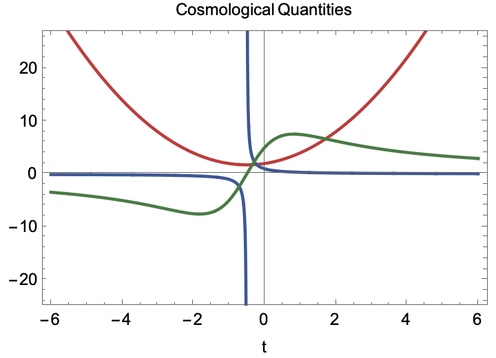
Figure 7: Evolutionary behavior for Eq. 4.24. The scale factor (red). The Hubble parameter amplified by an order of magnitude (green). The co-moving Hubble radius (blue). Model parameters: $a_{0}=b=1$, $c=2$.

The Ricci scalar and Kretchsmann scalar are given by:

$$R=\frac{6\left(b^{2}+6a_{0}bt+2a_{0}(c+3a_{0}t^{2})\right)}{(c+t(b+a_{0}t))^{2}}\,,\qquad K=\frac{12\left((b+2a_{0}t)^{4}+4a_{0}^{2}(c+t(b+a_{0}t))^{2}\right)}{(c+t(b+a_{0}t))^{4}}\,.$$ (4.28)

The absence of curvature singularities is shown from the curvature invariants plotted in Fig. 8

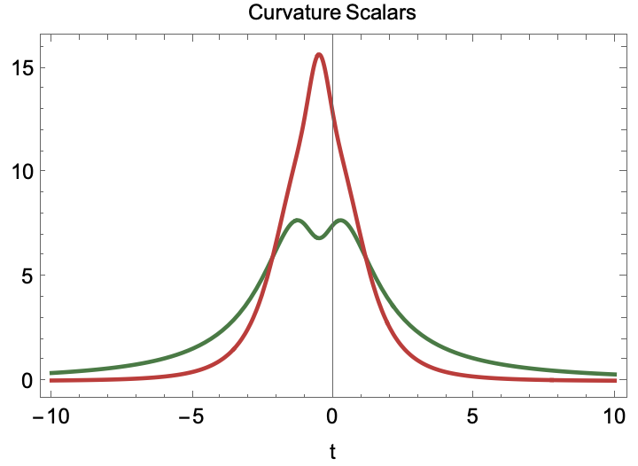
Figure 8: Curvature invariants computed in Eq. 4.28. The Ricci scalar (green) and the Kretchmann scalar (red). Model parameters: $a_{0}=b=1$, $c=2$.

Calculation of the Einstein tensor yields non-vanishing components:

$$G_{tt} = \frac{3(b+2a_{0}t)^{2}}{(c+t(b+a_{0}t))^{2}}\,,$$

$$G_{ii} = -b^{2}-8a_{0}bt-4a_{0}\left(c+2a_{0}t^{2}\right)\,.$$ (4.29)

The energy density is given by $\rho=-G^{t}{}_{t}$ and the pressure is $p=G^{i}{}_{i}$. A plot elucidating the energy conditions is given in Fig. 9

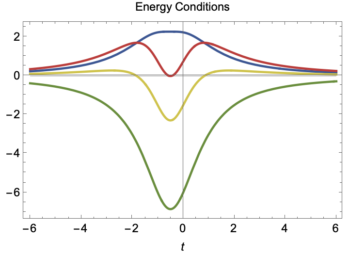
Figure 9: Energy conditions from Eq. IV.2.1. Plot of energy density $\rho$ (red), $\rho+p$ (yellow), $|p|$ (blue) and $\rho+3p$ (green). Model parameters: $a_{0}=b=1$, $c=2$.

While all of the classic energy conditions are violated, violation of the NEC can be restricted to an arbitrarily short time interval near the bounce point. Because of this, the asymptotic regions may be broken up into those obeying the NEC and the region violating the NEC.

In this model, and others we consider, the NEC is violated during a finite time interval, $-t_{-}<t<t_{+}$. One may break up the ANEC integral into the asymptotic regions $t<-t_{-}$, $t>t_{+}$ where other energy conditions ( e.g. NEC, WEC and DEC) are satisfied, and the NEC violating region. In this case the ANEC condition Eq. 1.1 may be recast as Giovannini (2017):

$$\left|\int_{t_{-}}^{t_{+}}(\rho+p)d\lambda\right|\leq\int_{-\infty}^{-t_{-}}(\rho+p)d\lambda+\int_{t_{+}}^{+\infty}(\rho+p)d\lambda\,,$$ (4.30)

where in the above we assume the spacetime curvature invariants are all regular and that the non-spacelike (causal) geodesics are complete and extendible to arbitrary values of their affine parameter. This is the case in all eternal universe solutions we present in this paper. In the energy condition plot, any violation of the ANEC may be ascertained via the inequality Eq. 4.30, each term being conveniently associated to an area beneath the curves defined by $\rho+p$ in the NEC violating, and NEC satisfying regions.

In this case the ANEC is found to be satisfied since,

$$\int_{-\infty}^{\infty}(\rho+p)d\lambda=-\frac{2(b+2a_{0}t)}{c+t(b+a_{0}t)}\Big{|}_{-\infty}^{\infty}=0\,.$$ (4.31)

In the late universe, only the SEC is violated allowing continued acceleration, as indicated by the negativity of the green curve. This too is an eternally inflating, bouncing cosmology similar to the behavior of Eq. 4.16, but it is better-behaved with respect to energy conditions as the NEC violation may be restricted to a moment in the very early universe , and the ANEC Eqs. 1.1 and 4.30 is satisfied.

IV.2.2 Models from limiting curvature

One method for building such non-singular bounces stems from the limiting curvature hypothesis (LCH) which stipulates the existence of minimal length (or maximal curvature) scale in nature, presumably somewhere near the Planck length Markov (1982, 1987), although one may introduce new physics at lower energy scales using this method. By construction, curvature invariants are limited in an action resulting in non-singular solutions. The LCH has been used to successfully construct many non-singular cosmological solutions Mukhanov and Brandenberger (1992); Brandenberger et al. (1993); Moessner and Trodden (1995); Brandenberger (1995); Brandenberger et al. (1998); Easson and Brandenberger (1999); Easson (2003a); Chamseddine and Mukhanov (2017a) in a variety of settings, as well as non-singular black hole solutions Frolov et al. (1989, 1990); Morgan (1991); Trodden et al. (1993); Easson (2003b, 2018); Chamseddine and Mukhanov (2017b); Brandenberger et al. (2021); Frolov and Zelnikov (2022).

A particular example following from the LCH is given by the scale factor Chamseddine and Mukhanov (2017a):

$$a(t)=a_{0}\left(c+bt^{2}\right)^{1/3}\,,$$ (4.32)

for constants $c>0,b>0$, which is capable of smoothly connecting two matter dominated phases having $a\propto t^{2/3}$ via a NEC violating bounce at $t=0$ where $\ddot{a}>0$. The schematic behavior of the cosmological quantities and the energy conditions are very similar to the polynomial model analyzed above; however, in the present case, even the SEC is obeyed in both the early and late (non-accelerating) universe. The ANEC Eqs. 1.1 and 4.30 is satisfied:

$$\int_{-\infty}^{\infty}(\rho+p)d\lambda=-\frac{4bt}{3(c+bt^{2})}\Big{|}_{-\infty}^{\infty}=0\,.$$ (4.33)

V An eternal loitering universe

We now discuss the possibility of an eternal loitering universe Sahni et al. (1992); Alexander et al. (2000); Brandenberger et al. (2002); Melcher et al. (2023). We break this section into two model categories, those which actually have an extended past Minkowski phase with $H=0$, and those which are always expanding, but have an extremely slow initial expansion asymptotically approaching Minkowski in the past. The latter we refer to as “quasi-loitering” models.

V.1 Loitering eternal universe

It is possible to construct a loitering eternal universe by smoothly gluing together a long Minkowski past phase to an inflating phase via a smooth bump function. This blueprint was first utilized in our previous work Lesnefsky et al. (2023b) to build a loitering model which is complete.

For this example we take the scale factor to be constant for $t<0$, so that $H=0\,\forall t<0$, and the spacetime is Minkowski. For $t>1$, the scale factor is exponential, $H$ is constant and the spacetime is qausi-de Sitter. A smooth bump function is used to piece the two regimes together in the regime $t\in[0,1]$.

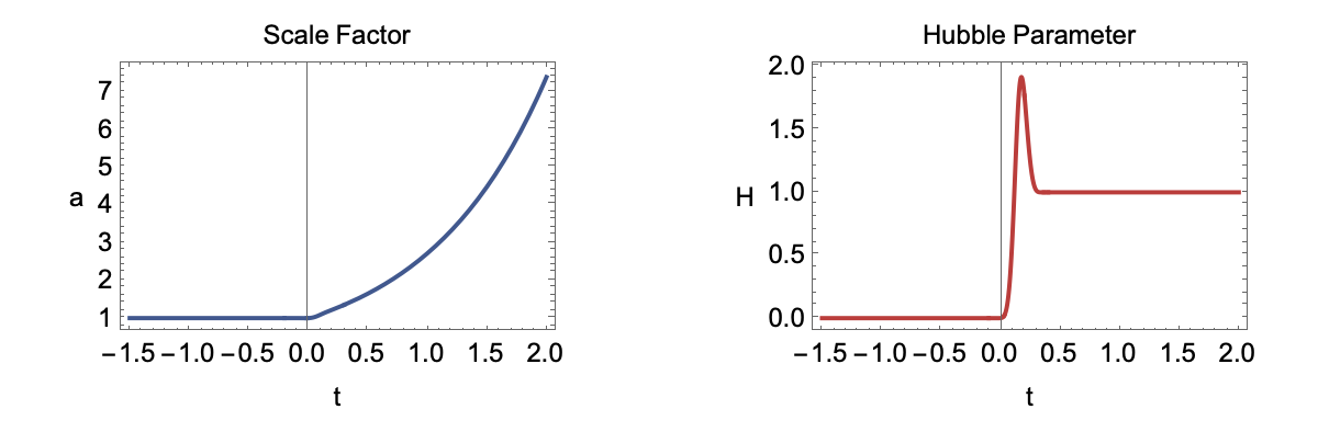
Figure 10: Evolutionary behavior for the loitering eternal model of §V.1.

Clearly the model is eternal and complete. As with previous examples, the NEC is violated when $\dot{H}>0$, and inflationary by Defn. 1 with $\ddot{a}>0$ for $t>0$. The ANEC Eq. 1.1 is satisfied. The Minkowski period with $H=0$ satisfies the bouncing conditions with $\dot{a}=0$ and with non-trivial scale factor overall, of Defn. 2. The model has an accelerating de Sitter phase at late times with $H=const$.

Using this technique it is simple to build an infinite number of interesting eternal and complete cosmological spacetimes. A category of geodesically complete spacetimes which we do not focus on here are cyclic models which are defined by multiple repeating bounces (see e.g. Penrose (2014); Steinhardt and Turok (2002); Steinhardt et al. (2002); Khoury et al. (2004); Ijjas and Steinhardt (2019); Lehners and Steinhardt (2013)). Such models are easy to construct using the above composite method. We dedicate further study of such composite spacetimes to future work Easson and Lesnefsky (to appear, 2024).

V.2 Quasi-loitering eternal universe

For our final example of an eternal universe we construct what we refer to as a quasi-loitering universe in that the scale factor is always expanding, although initially at an exponentially small (yet accelerated) rate before entering an increased accelerated inflationary phase. The situation at early time is reminiscent of the so-called Galileon Genesis model Creminelli et al. (2010), in which a universe that is asymptotically Minkowski in the past expands with $\dot{H}>H^{2}$, violating the NEC with an increasing energy density $\rho$; although, in the current model this phase naturally comes to an end. Eventually the inflationary phase transitions, the energy density decreases and the universe enters another period of extremely slow (negative accelerated) non-inflationary expansion. The quasi-loitering scale factor is:

$$a(t)=a_{0}\tanh\left(\frac{t}{\alpha}\right)+c\,.$$ (5.34)

In order to achieve geodesic completeness we require sufficient lifting of the tanh function, requiring $c>1$. The Hubble parameter is:

$$H=\frac{a_{0}\operatorname{sech}^{2}\left(\frac{t}{\alpha}\right)}{\alpha(c+a_{0}\tanh\left(\frac{t}{\alpha}\right))}\,.$$ (5.35)

At early times asymptotic into the past, as $t\rightarrow-\infty$, the universe is very slowly inflating. This inflation begins to increase with a sudden growing energy density (the continuity equation in GR gives $\dot{\rho}=-3H(\rho+p)$) and a strong NEC violating phase with $\dot{H}>0$, $\rho+p<0$. The acceleration equation gives:

$$\frac{\ddot{a}}{a}=-\frac{2a_{0}\operatorname{sech}^{2}\left(\frac{t}{\alpha}\right)\tanh\left(\frac{t}{\alpha}\right)}{\alpha^{2}(c+a_{0}\tanh\left(\frac{t}{\alpha}\right))}\,.$$ (5.36)

As $t\rightarrow\pm\infty$, the Hubble parameter approaches $H\rightarrow 0$. These zeros of $H$ are examples of bounce points at infinity as identified by Defn. 2, and hence, this is both an inflationary and a bouncing spacetime.

For the scale factor Eq. 5.34, it is possible to explicitly calculate the integrals of Thm 1. We find for the indefinite integrals:

$$\int^{t}\frac{a(\zeta)\,d\zeta}{\sqrt{\left(a(\zeta)\right)^{2}+1}}$$ (5.37)

$$=\frac{1}{2\alpha}\left(\frac{(a_{0}-c)\operatorname{arctanh}\left(\frac{1-a_{0}c+c^{2}+a_{0}(-a_{0}+c)\tanh\left(\frac{t}{\alpha}\right)}{\sqrt{1+(a_{0}-c)^{2}}\sqrt{1+c^{2}+a_{0}\tanh\left(\frac{t}{\alpha}\right)(2c+a_{0}\tanh\left(\frac{t}{\alpha}\right))}}\right)}{\sqrt{1+(a_{0}-c)^{2}}}\right.$$

$$\left.\quad+\frac{(a_{0}+c)\operatorname{arctanh}\left(\frac{1+c(a_{0}+c)+a_{0}(a_{0}+c)\tanh\left(\frac{t}{\alpha}\right)}{\sqrt{1+(a_{0}+c)^{2}}\sqrt{1+c^{2}+a_{0}\tanh\left(\frac{t}{\alpha}\right)(2c+a_{0}\tanh\left(\frac{t}{\alpha}\right))}}\right)}{\sqrt{1+(a_{0}+c)^{2}}}\right)$$

and

$$\int^{t}a\left(\zeta\right)d\zeta=ct+a_{0}\alpha\log\left(\cosh\left(\frac{t}{\alpha}\right)\right)\,.$$ (5.38)

As with our previous examples, the above integrals diverge over the full set of conditions discussed in Thm. 1 for all (non-zero) values of $\alpha$; hence, the spacetime is geodesically complete. The cosmological evolution is depicted in Fig. 11. Shown are the scale factor $a(t)$, Hubble parameter $H$ and co-moving Hubble radius $1/aH$. The inflation occurs at early times and eventually ends leading to a decelerating expanding phase with $\ddot{a}/a<0$. The future is a very slowly expanding (quasi-future-loitering) phase during which the energy conditions become well-behaved except the DEC is violated at late times and asymptotically approaches saturation, see Fig. 13.

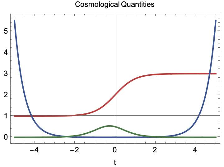
Figure 11: Evolutionary behavior for Eq. 5.34. The scale factor (red). The Hubble parameter (green). The co-moving Hubble radius suppressed by 1000 (blue). Model parameters: $a_{0}=\alpha=1$, $c=2$.

The Ricci scalar and Kretchsmann scalar are given by:

$$R = -\frac{6a_{0}\operatorname{sech}\left(\frac{t}{\alpha}\right)^{4}\left(a_{0}(-2+\cosh\left(\frac{2t}{\alpha}\right))+c\sinh\left(\frac{2t}{\alpha}\right)\right)}{\alpha^{2}(c+a_{0}\tanh\left(\frac{t}{\alpha}\right))^{2}}\,,$$

$$K = \frac{6a_{0}^{2}\operatorname{sech}\left(\frac{t}{\alpha}\right)^{8}\left(5a_{0}^{2}-c^{2}-4a_{0}^{2}\cosh\left(\frac{2t}{\alpha}\right)+(a_{0}^{2}+c^{2})\cosh\left(\frac{4t}{\alpha}\right)+16a_{0}c\cosh\left(\frac{t}{\alpha}\right)\sinh\left(\frac{t}{\alpha}\right)^{3}\right)}{\alpha^{4}(c+a_{0}\tanh\left(\frac{t}{\alpha}\right))^{4}}\,.$$

The absence of curvature singularities is shown from the curvature invariants plotted in Fig. 12

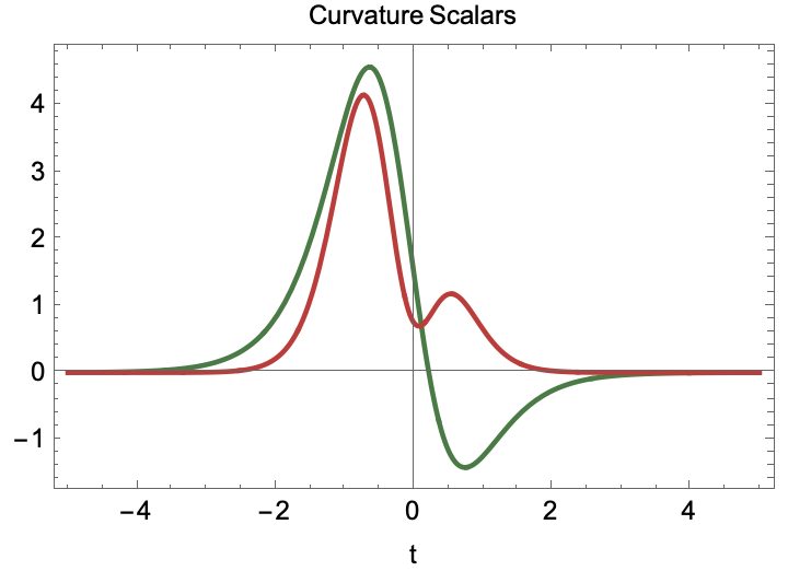
Figure 12: Curvature invariants computed from Eq. 5.34. The Ricci scalar (green) and the Kretchmann scalar (red). Model parameters: $a_{0}=\alpha=1$, $c=2$.

Calculation of the Einstein tensor yields non-vanishing components:

$$G_{tt} = -\frac{3a_{0}^{2}\operatorname{sech}^{4}\left(\frac{t}{\alpha}\right)}{\alpha^{2}(c+a_{0}\tanh\left(\frac{t}{\alpha}\right))^{2}}\,,$$

$$G_{ii} = \frac{a_{0}\operatorname{sech}^{4}\left(\frac{t}{\alpha}\right)\left(-3a_{0}+2a_{0}\cosh\left(\frac{2t}{\alpha}\right)+2c\sinh\left(\frac{2t}{\alpha}\right)\right)}{\alpha^{2}}\,.$$ (5.39)

The energy density is given by $\rho=-G^{t}{}_{t}$ and the pressure is $p=G^{i}{}_{i}$. A plot elucidating the energy conditions is given in Fig. 13.

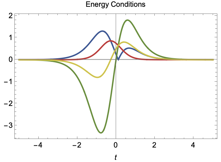
Figure 13: Energy conditions from Eq. V.2. Plot of energy density $\rho$ (red), $\rho+p$ (yellow), $|p|$ (blue) and $\rho+3p$ (green). Model parameters: $a_{0}=\alpha=1$, $c=2$.

At early times, all of the classical energy conditions are violated. At late times the WEC, NEC and SEC are all satisfied. Only the DEC is mildly violated at late times; however, there exists a brief period for small positive $t$, during which all of the energy conditions are satisfied. This period lasts from $t=0$ when the SEC (green curve) starts to be satisfied until the moment the blue curve grows larger than the red curve where the DEC begins to be violated. This healthy period can be past extended to accommodate an inflationary phase where only the SEC is violated (starting where NEC is valid and yellow curve intersects the horizontal line). The inflationary period naturally ends when the SEC starts to be obeyed (green curve intersects the horizontal line). For the ANEC, we evaluate Eq. 1.1

$$\int_{-\infty}^{\infty}(\rho+p)d\lambda=\frac{2a_{0}\tanh\left(\frac{t}{\alpha}\right)\left(a_{0}+c\tanh\left(\frac{t}{\alpha}\right)\right)}{c\alpha\left(c+a_{0}\tanh\left(\frac{t}{\alpha}\right)\right)}\Big{|}_{-\infty}^{\infty}=0\,,$$ (5.40)

for our model parameters. Hence, the ANEC is satisfied.

VI Discussion

Here we summarize our key findings. We see from the energy condition plots above that all of the models we have scrutinized embrace at least some period of null energy condition violation:

Conjecture 7.

In General Relativity, every smooth, non-constant scale factor a(t) of a geodesically complete FRW spacetime must violate the NEC for at least some period of time.

The above is obviously true for all bouncing FRW cosmological models. As is well-known, in a flat $k=0$ (or hyperbolic $k=-1$) FRW spacetime, the NEC must be violated in order to achieve a cosmological bounce Hawking and Penrose (1970). During a bounce through a local minimum, the universe transitions from a contracting phase, $H<0$, to an expanding phase, $H>0$. This transition inherently requires that at the point where the contraction halts and expansion begins, the derivative of the Hubble parameter, $\dot{H}$, must be positive. Since $\dot{H}=-4\pi G(\rho+p)$, we must have $\rho+p<0$, signalling violation of the NEC. Thus, any such spacetime which exhibits a bounce, or bounces, for any part of it’s history must violate NEC. Likewise any super-inflationary models (by definition) have $\dot{H}>0$ and violate NEC. With non-zero curvature $k$, one can produce a bounce without violating NEC since, $\dot{H}=-4\pi G(\rho+p)+k/a^{2}$, can become positive at the bounce due to positive $k$; however, such universes are closed if the matter sector obeys NEC. While the NEC holds, $\ddot{a}/a=H^{2}+\dot{H}=-4\pi G(\rho/3+p)$, and $H=0$ at the bounce, $\ddot{a}/a>0$ and the SEC is violated. Curvature bounces are discussed in detail in Starobinskii (1978); Graham et al. (2014).

Conjecture 7 clearly holds in the case of the general polynomial inflationary models given by Eq. 4.24. Any such model with non-constant scale factor that are complete will be inflationary by Corollary 4 and clearly contain (at least) one bounce (hence, violating the NEC).

It remains only to show that all models which are geodesically complete (in principle, do not bounce) and involve an inflationary phase of arbitrary length violate NEC; although, as one can see all of the above models satisfy our definition of a bouncing cosmology Defn. 2 (essentially, a place where $\dot{a}=0$). While most of the models demonstrate the bounce phase clearly, it is worth revisiting the eternal inflationary model Eq. 3.11, in this context.

Our exponential model Eq. 3.11, can be expanded in a Taylor expansion. The Maclaurin series of the relevant portion of the scale factor is

$$e^{\frac{2t}{\alpha}}=\sum_{n=0}^{\infty}\frac{\left(\frac{2t}{\alpha}\right)^{n}}{n!}=1+\frac{2t}{\alpha}+\frac{\left(\frac{2t}{\alpha}\right)^{2}}{2!}+\frac{\left(\frac{2t}{\alpha}\right)^{3}}{3!}+\cdots\,,$$ (6.41)

and is compatible with Eq. 4.23. Applied to the scale factor Eq. 3.11, the odd powered polynomial terms are negative as $t\rightarrow-\infty$, and effectively cancel the positive even powered terms ultimately creating a “bounce point at infinity” in accordance with Defns. 2,3 at $t\rightarrow-\infty$, with constant scale factor $a=c$ and with $H=0$. Thus, our eternal inflating model Eq. 3.11 is also a bouncing cosmology par Defn.2. To elucidate our discussion we remind the reader of the general polynomial bounce discussed in §IV.2 and Eqs. 4.23 and 4.24. In essence the bounce point of a finite series polynomial, such as Eq. 4.24, is in this case translated to $t\rightarrow-\infty$, where

$$\lim_{t\rightarrow-\infty}H=0\,.$$ (6.42)

In further support of this notion of the “bounce”, one sees that the bouncing cosh model Eq. 4.16, having $\dot{a}(t_{0})=0$ at the bounce point, is recovered by adding together two copies of the exponential model Eq. 3.11, one with $\alpha>0$ and one with $\alpha<0$, each having its own “bounce at infinity” at $t=\pm\infty$ where $H=0$:

$$a_{0}\,e^{\frac{2t}{\alpha}}+c+a_{0}\,e^{\frac{-2t}{\alpha}}+c=2\left(c+a_{0}\cosh\left(\frac{2t}{\alpha}\right)\right)\,.$$ (6.43)

On the path to $t=+\infty$, we find all terms in the polynomial expansion Eq. 6.41 are positive, and sum to give a de Sitter inflating phase with constant $H$:

$$\lim_{t\rightarrow\infty}H=2/\alpha\,.$$ (6.44)

Indeed, all of the geodesically complete spacetimes presented have at least some period of NEC violation, and a phase with $\dot{a}=0$, and may be classified as bouncing models in accordance with Defn. 2:

Conjecture 8.

In General Relativity, every smooth, non-constant scale factor a(t) of a geodesically complete FRW spacetime must experience at least one bounce.

Combining this with Cors.4,6 and Conj.5, we formulate a provocative composite conjecture:

Conjecture 9.

Every geodesically complete eternal spacetime which admits a neighborhood isometric to a GFRW with a non-constant scale factor will inflate for some time and bounce at least once.

Naturally, the question of whether our own observable universe started with an inflationary phase or cosmological bounce is of paramount importance; however, ultimately, in the context of an inflationary model, our access to primordial perturbations is limited to a small number of e-foldings, as discerned through observations of the cosmic microwave background (CMB). Observables from the early universe capable of probing and constraining models are plentiful and include primordial gravitational waves, non-gaussianities, isocurvature modes, various reheating predictions, of course the two-point correlation power spectrum and others Mather et al. (1990); Daly (1991); Mather et al. (1994); Hu et al. (1994); Linde and Mukhanov (1997); Moroi and Takahashi (2001); Lyth and Wands (2002); Smith et al. (2006a, b); Hinshaw et al. (2013); Dent et al. (2012); Cook et al. (2015); Aghanim et al. (2020). Incredible progress has been made in detecting or attempting to detect these observables and we remain optimistic with respect to eventually identifying the underlying mechanisms responsible for generating our universe. But there are many technical challenges ahead, and limited data can make it difficult to definitively distinguish between bouncing and inflationary models due to degeneracy problems Easson and Powell (2011a, b, 2013); Vennin et al. (2015); Mishra et al. (2021); Ben-Dayan and Thattarampilly (2023), or other obstructions. 

In our discussion of a fully geodesically complete spacetime that exists for an eternity, we encounter a tautological paradigm shift: the key focus moves from categorizing spacetimes as “inflationary” or “bouncing” to emphasizing their geodesic completeness. We discover from Conj. 9, although both inflation and cosmological bounces play crucial roles in forming a geodesically complete spacetime, they are often transient stages in the vast timeline of an eternal cosmos. 

Developing a comprehensive model for an eternal universe goes far beyond the initial explorations presented here, requiring studies of anisotropic models and a move away from the simplistic perfect fluid description. One must incorporate our known observable universe with a proper reheating period, nucleosynthesis, and periods of radiation, matter and dark energy domination. This ambitious endeavor awaits those venturing along future-directed (hopefully complete) timelike geodesic rays.

Appendix A Energy conditions

For this discussion we will assume General Relativity with matter described by a perfect fluid stress energy tensor

$$T_{\mu\nu}=(\rho+p)U_{\mu}U_{\nu}+pg_{\mu\nu}\,,$$ (1.45)

where $p$ and $\rho$ and the pressure and energy density of the fluid and $U^{\mu}$ is the fluid four-velocity.

A.1 Weak Energy Condition (WEC)

The WEC states that $T_{\mu\nu}t^{\mu}t^{\nu}\geq 0$, $\forall$ timelike vectors $t^{\mu}$. This is equivalent to $\rho\geq 0$ and $\rho+p\geq 0$.

A.2 Null Energy Condition (NEC)

The NEC states that $T_{\mu\nu}\ell^{\mu}\ell^{\nu}\geq 0$, $\forall$ null vectors $\ell^{\mu}$. This is equivalent to $\rho+p\geq 0$. The energy density may now be negative as long as it is compensated for by sufficient positive pressure.

A.3 Dominant Energy Condition (DEC)

The DEC states that $T_{\mu\nu}t^{\mu}t^{\nu}\geq 0$, $\forall$ timelike vectors $t^{\mu}$ as well as $T_{\mu\nu}T^{\nu}{}_{\lambda}t^{\mu}t^{\lambda}\leq 0$. This is equivalent to $\rho\geq|p|$.

A.4 Strong Energy Condition (SEC)

The SEC states that $T_{\mu\nu}t^{\mu}t^{\nu}\geq\frac{1}{2}T^{\lambda}{}_{\lambda}t^{\sigma}t_{\sigma}$, $\forall$ timelike vectors $t^{\mu}$. This is equivalent to $\rho+p\geq 0$ and $\rho+3p\geq 0$.

Note that the DEC$\implies$WEC, WEC$\implies$NEC, SEC$\implies$NEC; and SEC$\hbox to0.0pt{$\quad\not$\hss}\implies$WEC.

Appendix B Theorem 1 Item 3 Proof

The denominators of Eqs. 2.6 and 2.7 in the spacelike case of $w_{0}=-1$ evaluate to $\sqrt{1-a^{2}\left(t\right)}$. We now invoke an (enthymeme) assumption that the domain of discourse of this proof exists for real valued differentiable manifolds, so $\sup_{\mathbb{R}^{1}_{1}}a=1$ if the denominator is to evaluate to a real number between $\left[0,1\right]$ and not become imaginary. We now have 3 cases; unlike the timelike case where there are two disconnected lightcones (hence, two integral orientations $\int_{t_{0}}^{\infty}$ and $\int^{t_{0}}_{-\infty}$), the null case, despite the fact that the null cone is connected one remains either future pointing or past pointing, the unit spacelike hyperquadratic in $T_{p}\mathcal{M}$ under the exponential map $\exp_{p}$ is connected with potential (closed) periodic spacelike curves. There are 3 subcases: $d\pi_{\mathbb{R}^{1}_{1}}\dot{\gamma}=\frac{dt}{d\lambda}\frac{\partial}{\partial t}$ is future directed, past directed, or purely spacelike (achronal). In the achronal case, the geodesic is complete by the assumption that $\left(\Sigma,g_{\Sigma}\right)$ is complete. In both the past and future cases, the integrand of $\frac{a}{\sqrt{1-a^{2}}}>a$ is pointwise $\forall\alpha\in\mathbb{R}^{1}_{1}$ because $\sqrt{1-a^{2}}<1$ by the spacelike assumption and the assumption that this is a $\mathbb{R}$ valued differentiable manifold. Thus, if the null integral diverges so will the spacelike integrals. There is one more technicality to consider, that of periodic spacelike geodesics. In this case, the integrands are everywhere strictly positive, so with every period another strictly positive mass is added to the integral, and as the number of orbits becomes unbounded approaching cardinal $\aleph_{0}$, the integral diverges.

Considering this, a periodic spacelike trajectory will have $d\pi_{\mathbb{R}^{1}_{1}}\dot{\gamma}=\frac{dt}{d\lambda}\frac{\partial}{\partial t}$, partially future pointing and partially past pointing so that the two distinct past (future) directed integrals coincide. For the case of unbounded trajectories, if the null integral diverges so will the two past (future) pointing spacelike integrals, for the reason mentioned above. Thus, for spacelike completeness, one must be both past (future) null complete - along with the achronal case which holds by assumption - so full null completeness must hold. The null case of the integral of item (2) bounds the non-infinite $a$ spacelike case from below. Thus, if the GFRW is past and / or future null complete then - in the case of a non-infinite $a$ - the GFRW is spacelike complete and the first portion of item (3) is proven. For completeness, we include the case where $a$ potentially diverges and becomes infinite for a finite $t\in\mathbb{R}$. In this case a “big rip” boundary will form and a geodesic will encounter it within finite parameter.

Finally, as a matter of definition, a Lorentzian spacetime is (fully) geodesically complete if every geodesic ray is both past and future, timelike, null, and spacelike complete; thus, item (5) is proven.

Appendix C Generalized Robertson Walker Spacetimes

The well-known Friedmann Robertson Walker (FRW) spacetime can be extended to a Generalized Friedmann Robertson Walker (GFRW) spacetime construction. Many properties of FRW spacetimes do not utilize the spaceform homogeniety and isotropy of the spatial section and are predicated upon behavior of the scale factor only. The constant sectional curvature assumptions of the FRW spatial sections can be weakened to any complete Riemannian manifold.

C.1 Definition

Building on the warped product formalism of Bishop and O’Neill (1969) defined for Riemannian manifolds, it can be repurposed and melded with the FRW formalism to define a Generalized Friedmann Robertson Walker spacetime as in O’Neill (1983); Sanchez (1998); Romero and Sanchez (1994).

Definition 4.

Let $\mathbb{R}^{1}_{1}$ be the negative definite manifold $\left(\mathbb{R},-dt^{2}\right)$ and $\left(\Sigma,g_{\Sigma}\right)$ be any geodesically complete Riemannian manifold, and $a\in\mathcal{C}^{\infty}\left(\mathbb{R}^{1}_{1}\right)$ a smooth, strictly positive function on $\mathbb{R}$. A Generalized Robertson Walker spacetime, denoted $\mathbb{R}^{1}_{1}\times_{a}\Sigma$, is the (topological) Cartesian product $\mathbb{R}^{1}_{1}\times\Sigma$ with metric $d\pi^{*}_{\mathbb{R}^{1}_{1}}\left(-dt^{2}\right)+a^{2}\left(t\right)d\pi^{*}_{\Sigma}g_{\Sigma}$ where $\pi_{\mathbb{R}^{1}_{1}}$, $\pi_{\Sigma}$ are the canonical projections onto $\mathbb{R}^{1}_{1}$, $\Sigma$ guaranteed by the Cartesian product construction. From this point on, unless otherwise required, the metric pullbacks $d\pi^{*}_{\mathbb{R}^{1}_{1}}\left(-dt^{2}\right)$, $d\pi^{*}_{\Sigma}g_{\Sigma}$ will have $d\pi^{*}_{\mathbb{R}^{1}_{1}}$, $d\pi^{*}_{\Sigma}g_{\Sigma}$ omitted.

For enumerated derived properties of the connection, geodesics, and curvatures of GFRWs see O’Neill (1983) Chapters 7,12. Here we now show how GFRW geodesic equation projections relate to the common geodesic equation

$$\frac{d^{2}x^{\sigma}}{d\lambda^{2}}+\Gamma^{\sigma}_{\alpha\beta}\frac{dx^{\alpha}}{d\lambda}\frac{dx^{\beta}}{d\lambda}=0\,.$$ (3.46)

C.2 Geodesics in GFRWs

Let $\mathcal{M}=\mathbb{R}^{1}_{1}\times_{a}\Sigma$ be a GFRW and $x^{\mu}\left(\lambda\right)=t\left(\lambda\right)\oplus x^{k}\left(\lambda\right)$ be a geodesic having affine parameter $\lambda$ with $t=\pi_{\mathbb{R}^{1}_{1}}x^{\mu}$ being the (timelike) projection on $\mathbb{R}^{1}_{1}$, and $x^{k}=\pi_{\Sigma}x^{\mu}$ being the (spacelike) projection on $\left(\Sigma,g_{\Sigma}\right)$. The geodesic equation as viewed in $\mathcal{M}$:

$$\nabla_{\frac{dx^{\nu}}{d\lambda}\frac{\partial}{\partial x^{\nu}}}\frac{dx^{\mu}}{d\lambda}\frac{\partial}{\partial x^{\mu}}=\left(\frac{d^{2}x^{\mu}}{d\lambda^{2}}+\Gamma^{\mu}_{\alpha\beta}\frac{dx^{\alpha}}{d\lambda}\frac{dx^{\beta}}{d\lambda}\right)\frac{\partial}{\partial x^{\mu}}=0$$ (3.47)

The full geodesic equation in $\mathcal{M}$ can be projected into both $\mathbb{R}^{1}_{1},\left(\Sigma,g_{\Sigma}\right)$ as differential equations:

$$\nabla_{\frac{\partial}{\partial t}}\frac{\partial}{\partial t}=-g_{\Sigma}\left(\frac{dx^{k}}{d\lambda}\frac{\partial}{\partial x^{k}},\frac{dx^{k}}{d\lambda}\frac{\partial}{\partial x^{k}}\right)\cdot\left(a\left(t\left(\lambda\right)\right)\right)\cdot\frac{da}{dt}$$ (3.48)

$$\nabla_{\left(\frac{dx^{k}}{d\lambda}\frac{\partial}{\partial x^{k}}\right)}\left(\frac{dx^{\ell}}{d\lambda}\frac{\partial}{\partial x^{\ell}}\right)=-\frac{2}{a\left(t\left(\lambda\right)\right)}\frac{da}{dt}\frac{dt}{d\lambda}\frac{dx^{\ell}}{d\lambda}\frac{\partial}{\partial x^{\ell}}$$ (3.49)

respectively. In particular, Eq. 3.49 in $\Sigma$ is not quite totally geodesic, but is a pregeodesic because the acceleration is proportional to $\frac{dx^{\ell}}{d\lambda}\frac{\partial}{\partial x^{\ell}}$ and thus a geodesic reparameterization exists “boosting” away the acceleration the affine parameter $\lambda$. The image of Eq. 3.49 is the image of a geodesic. We now invoke the completeness assumption of $\left(\Sigma,g_{\Sigma}\right)$, yielding $x^{k}\left(\lambda\right)$ is defined $\forall\,\mathbb{R}$. Finally, if $x^{\mu}\left(\lambda\right)$ fails to be complete, it must be due to Eq. 3.48.

C.3 Derivation of Warped Product Geodesics

In fact, Eqs. 3.48 and 3.49 can be generalized to a warped product of any semi-Riemannian manifolds. The familiar geodesic equation Eq. 3.46 can be distilled into the generalized form of Eqs. 3.48 and 3.49. In the following we use $f$ for the scale factor. As in O’Neill (1983) Chapter 7 in a warped product of any two semi-Riemannian manifolds $B\times_{f}F$ the first manifold is the leaf manifold $\left(B,\tilde{g}_{B}\right)$ - corresponding to $\mathbb{R}^{1}_{1}$ - and the second manifold is the fiber $\left(F,\tilde{g}_{F}\right)$ - corresponding to $\left(\Sigma,g_{\Sigma}\right)$. Additionally, consider a chart $\left(U_{B},\{t^{k}\}\right)$ of $B$ and a chart $\left(U_{F},\{x^{\ell}\}\right)$. The warped product metric is a block diagonal form $g_{B}+f^{2}\left(t^{k}\right)g_{F}$. All factors of $f\left(t^{k}\right)$ will be explicitly written and terms with a “tilde” are viewed to be elements of the constituent spaces and naked (no tilde) terms are elements of the warped product $B\times_{f}F$, for example the pullback $g_{B}=d\pi_{B}^{*}\tilde{g}_{B}$. Finally, the geodesic equation is calculated over curve $t^{k}\left(\lambda\right)\otimes x^{\ell}\left(\lambda\right)$.

For this construction, the Christoffel symbols can be calculated

$$\Gamma^{t^{k}}_{t^{\ell}t^{m}} =\tilde{\Gamma}^{t^{k}}_{t^{\ell}t^{m}} \Gamma^{t^{k}}_{x^{\ell}x^{m}} =-\left(\tilde{g}_{F}\right)_{x^{\ell}x^{m}}f\left(t^{k}\right)\mathrm{grad}_{\tilde{g}_{B}}f \Gamma^{t^{k}}_{t^{\ell}x^{m}} =0$$

$$\Gamma^{x^{k}}_{x^{\ell}x^{m}} =\tilde{\Gamma}^{x^{k}}_{x^{\ell}x^{m}} \Gamma^{x^{k}}_{x^{\ell}t^{m}} =\frac{1}{f\left(t^{m}\right)}\frac{\partial f}{\partial t^{m}}\left(\tilde{g}_{F}\right)^{x^{k}x^{a}}\left(\tilde{g}_{F}\right)_{x^{a}x^{\ell}} \Gamma^{x^{k}}_{t^{\ell}t^{m}} =0$$

The geodesic equation may be expanded

$$0 =\frac{d^{2}x^{\sigma}}{d\lambda^{2}}+\Gamma^{\sigma}_{\alpha\beta}\frac{dx^{\alpha}}{d\lambda}\frac{dx^{\beta}}{d\lambda}$$

$$=\frac{d^{2}t^{k}}{d\lambda^{2}}+\Gamma^{t^{k}}_{\alpha\beta}\frac{dx^{\alpha}}{d\lambda}\frac{dx^{\beta}}{d\lambda}+\frac{d^{2}x^{\ell}}{d\lambda^{2}}+\Gamma^{x^{\ell}}_{\alpha\beta}\frac{dx^{\alpha}}{d\lambda}\frac{dx^{\beta}}{d\lambda}$$

$$=\frac{d^{2}t^{k}}{d\lambda^{2}}+\Gamma^{t^{k}}_{t^{a}t^{m}}\frac{dt^{a}}{d\lambda}\frac{dt^{m}}{d\lambda}+\Gamma^{t^{k}}_{x^{a}x^{m}}\frac{dx^{a}}{d\lambda}\frac{dx^{m}}{d\lambda}$$

$$\qquad+\frac{d^{2}x^{\ell}}{d\lambda^{2}}+\Gamma^{x^{\ell}}_{x^{a}x^{m}}\frac{dx^{a}}{d\lambda}\frac{dx^{m}}{d\lambda}+\Gamma^{x^{\ell}}_{x^{a}t^{m}}\frac{dx^{a}}{d\lambda}\frac{dt^{m}}{d\lambda}+\Gamma^{x^{\ell}}_{t^{a}x^{m}}\frac{dt^{a}}{d\lambda}\frac{dx^{m}}{d\lambda}$$

$$=\frac{d^{2}t^{k}}{d\lambda^{2}}+\tilde{\Gamma}^{t^{k}}_{t^{a}t^{m}}\frac{dt^{a}}{d\lambda}\frac{dt^{m}}{d\lambda}-\left(\left(\tilde{g}_{F}\right)_{x^{\ell}x^{m}}\frac{dx^{a}}{d\lambda}\frac{dx^{m}}{d\lambda}\right)\cdot\left(f\left(t^{k}\right)\mathrm{grad}_{\tilde{g}_{B}}f\right)$$

$$\qquad+\frac{d^{2}x^{\ell}}{d\lambda^{2}}+\tilde{\Gamma}^{x^{\ell}}_{x^{a}x^{m}}\frac{dx^{a}}{d\lambda}\frac{dx^{m}}{d\lambda}+\frac{2}{f\left(t^{m}\right)}\frac{\partial f}{\partial t^{m}}\left(\tilde{g}_{F}\right)^{x^{\ell}x^{a}}\left(\tilde{g}_{F}\right)_{x^{a}x^{k}}\frac{dx^{a}}{d\lambda}\frac{dt^{m}}{d\lambda}$$ (3.50)

One then notes that the $t^{k}$ terms and $x^{\ell}$ terms in the final expression of Eq. C.3 are linearly independent, so for the geodesic equation to be homogeneous each vector term must be homogeneous. Thus

$$\frac{d^{2}t^{k}}{d\lambda^{2}}+\tilde{\Gamma}^{t^{k}}_{t^{a}t^{m}}\frac{dt^{a}}{d\lambda}\frac{dt^{m}}{d\lambda}=\left(\left(\tilde{g}_{F}\right)_{x^{\ell}x^{m}}\frac{dx^{a}}{d\lambda}\frac{dx^{m}}{d\lambda}\right)\cdot\left(f\left(t^{k}\right)\mathrm{grad}_{\tilde{g}_{B}}f\right)$$ (3.51)

$$\frac{d^{2}x^{\ell}}{d\lambda^{2}}+\tilde{\Gamma}^{x^{\ell}}_{x^{a}x^{m}}\frac{dx^{a}}{d\lambda}\frac{dx^{m}}{d\lambda}=-\frac{2}{f\left(t^{m}\right)}\frac{\partial f}{\partial t^{m}}\delta^{x^{\ell}}_{x^{k}}\frac{dx^{k}}{d\lambda}\frac{dt^{m}}{d\lambda}$$ (3.52)

are recovered. In order to eventually compare Eqs. 3.51, 3.52 to Eqs. 3.48, 3.49 in the case of a GFRW one can consolidate using formal notation 

$$\nabla_{\left(\frac{dt^{\ell}}{d\lambda}\frac{\partial}{\partial t^{\ell}}\right)}\left(\frac{dt^{\ell}}{d\lambda}\frac{\partial}{\partial t^{\ell}}\right)=\tilde{g}_{F}\left(\frac{dx^{k}}{d\lambda}\frac{\partial}{\partial x^{k}},\frac{dx^{m}}{d\lambda}\frac{\partial}{\partial x^{m}}\right)\cdot\left(f\left(t^{\ell}\right)\mathrm{grad}_{\tilde{g}_{B}}f\right)$$ (3.53)

$$\nabla_{\left(\frac{dx^{\ell}}{d\lambda}\frac{\partial}{\partial x^{\ell}}\right)}\left(\frac{dx^{\ell}}{d\lambda}\frac{\partial}{\partial x^{\ell}}\right)=-\frac{2}{f\left(t^{m}\right)}\frac{\partial f}{\partial t^{m}}\frac{dt^{m}}{d\lambda}\frac{dx^{k}}{d\lambda}\frac{\partial}{\partial x^{k}}$$ (3.54)

In the case of a GFRW, $\left(B,\tilde{g}_{B}\right)=\mathbb{R}^{1}_{1}$ and $\left(F,\tilde{g}_{F}\right)=\left(\Sigma,g_{\Sigma}\right)$; with respect to Eqs. 3.53, 3.54 the aforementioned Eqs. 3.48, 3.49 are recovered, as desired.

C.4 A Useful Constant

The question of notation nonwithstanding, Eqs. 3.51, 3.52, Eqs. 3.53, 3.54, and / or Eqs. 3.48, 3.49 form a system of coupled ODEs which, at least upon a cursory inspection, appear formidable. However, they can be simplified with the introduction of a geodesic dependent constant.

Given a geodesic $t^{\ell}\left(\lambda\right)\oplus x^{k}\left(\lambda\right)$ a constant

$$\xi^{2}_{t^{\ell}\oplus x^{k}}=f^{4}\left(t^{\ell}\right)\tilde{g}_{F}\left(\frac{dx^{k}}{d\lambda}\frac{\partial}{\partial x^{k}},\frac{dx^{k}}{d\lambda}\frac{\partial}{\partial x^{k}}\right)$$ (3.55)

can be defined along the image of the geodesic. The constant $\xi^{2}_{t^{\ell}\oplus x^{k}}$ is not a Noether conserved quantity a propos any symmetry per se, but represents the initial spatial “speed” of a particle in “free fall” upon a geodesic.

Proof.

Starting with geodesic $t^{\ell}\left(\lambda\right)\oplus x^{k}\left(\lambda\right)$ with velocity vector $\frac{d}{d\lambda}$ one calculates along the image of $t^{\ell}\left(\lambda\right)\oplus x^{k}\left(\lambda\right)$:

$$\frac{d\xi^{2}_{t^{\ell}\oplus x^{k}}}{d\lambda} \overset{?}{=}\frac{d}{d\lambda}\left[f^{4}\left(t^{\ell}\right)\tilde{g}_{F}\left(\frac{dx^{k}}{d\lambda}\frac{\partial}{\partial x^{k}},\frac{dx^{k}}{d\lambda}\frac{\partial}{\partial x^{k}}\right)\right]$$

$$=4f^{3}\left(t^{\ell}\right)\frac{df}{dt^{\ell}}\frac{dt^{\ell}}{d\lambda}\tilde{g}_{F}\left(\frac{dx^{k}}{d\lambda}\frac{\partial}{\partial x^{k}},\frac{dx^{k}}{d\lambda}\frac{\partial}{\partial x^{k}}\right)+2f^{4}\left(t^{\ell}\right)\tilde{g}_{F}\left(\nabla_{\frac{d}{d\lambda}}\frac{dx^{k}}{d\lambda}\frac{\partial}{\partial x^{k}},\frac{dx^{k}}{d\lambda}\frac{\partial}{\partial x^{k}}\right)$$

$$=4f^{3}\left(t^{\ell}\right)\frac{df}{dt^{\ell}}\frac{dt^{\ell}}{d\lambda}\tilde{g}_{F}\left(\frac{dx^{k}}{d\lambda}\frac{\partial}{\partial x^{k}},\frac{dx^{k}}{d\lambda}\frac{\partial}{\partial x^{k}}\right)-4\frac{f^{4}\left(t^{\ell}\right)}{f\left(t^{\ell}\right)}\tilde{g}_{F}\left(\frac{dx^{k}}{d\lambda}\frac{\partial}{\partial x^{k}},\frac{dx^{k}}{d\lambda}\frac{\partial}{\partial x^{k}}\right)$$

$$=0$$

where Eq. 3.49 was inserted to evaluate $\nabla_{\frac{d}{d\lambda}}\frac{dx^{k}}{d\lambda}\frac{\partial}{\partial x^{k}}$. ∎

Utilizing $\xi^{2}_{t^{\ell}\oplus x^{k}}$ one can revisit Eq. 3.48. The potentially complex - even before integration! - term $f\left(t^{\ell}\right)\tilde{g}_{F}\left(\frac{dx^{k}}{d\lambda}\frac{\partial}{\partial x^{k}},\frac{dx^{k}}{d\lambda}\frac{\partial}{\partial x^{k}}\right)$ can be eliminated for $\frac{\xi^{2}_{t^{\ell}\oplus x^{k}}}{f^{3}\left(t^{\ell}\right)}$. The $\nabla_{\frac{\partial}{\partial t}}\frac{\partial}{\partial t}$ equation now reads

$$\nabla_{\frac{\partial}{\partial t}}\frac{\partial}{\partial t}=\frac{\xi^{2}_{t^{\ell}\oplus x^{k}}}{f^{3}\left(t^{\ell}\right)}\mathrm{grad}_{\tilde{g}_{B}}f$$ (3.56)

which has a more tractable integral solution: Thm 1 follows.

Appendix D A Diffeomorphism of the Real Line

Figure 14: Diffeomorphism of $\left(-\infty,\infty\right)$ and $\left(1,2\right)$. For the map to be smooth the derivatives at the tails must approach zero which necessitates an inflection change. The diffeomorphism displayed is $\frac{1}{\frac{1}{bb-aa}+AA^{-x}}+aa$ with $aa\mapsto 1$, $bb\mapsto 2$, and shape parameter $AA\mapsto 10$.

For the purpose of constructing a counter-example to the above conjecture one must be careful to preserve the required geodesic completeness of the scale factor. The scale factor must be defined for all $\mathbb{R}$ and have a strictly positive infimum. Thus, for the prescription to be a counter-example the diffeomorphism must compactify all $\mathbb{R}$ to the bounded interval where $-t^{2}+1>0$. Additionally, for the infinte to be compactified in a smooth fashion the derivative must approach zero on the asymptotes. The diffeomorphism, therefore, requires an inflection change. When said diffeomorphism is composed with the target concave down function, a balance of sort is created with the positive concavity of the diffeomorphism contrasting with the negative concavity of the target function. Although we have no formal proof this must always occur, in every calculation we have performed, we have always found at least a small interval where the positive inflection of the diffeomorphism wins out and the conjecture holds.

Finally, the smoothness assumption is important to rule out the piecewise linear case, where no concavity exists. Either a linear scale factor is unbroken and the positive definite requirement fails to hold or a broken linear scale factor fails to be smooth and contains singularities. A GFRW with a smooth scale factor is, by construction, free of curvature singularities. Thus, any non-trivial scale factor must be non-linear and can have at most a countable number of points with vanishing second derivative.

References

- Guth (1981) A. H. Guth, “The Inflationary Universe: A Possible Solution to the Horizon and Flatness Problems,” Phys. Rev. D 23, 347 (1981).
- Linde (1982) A. D. Linde, “A New Inflationary Universe Scenario: A Possible Solution of the Horizon, Flatness, Homogeneity, Isotropy and Primordial Monopole Problems,” Phys. Lett. B 108, 389 (1982).
- Albrecht and Steinhardt (1982) A. Albrecht and P. J. Steinhardt, “Cosmology for Grand Unified Theories with Radiatively Induced Symmetry Breaking,” Phys. Rev. Lett. 48, 1220 (1982).
- 198 (1983) Paul J. Steinhadt in, Very Early Universe: proceedings of the Nuffield workshop, Cambridge, 21 June to 9 July, 1982 (1983).
- Vilenkin (1983) Alexander Vilenkin, “The Birth of Inflationary Universes,” Phys. Rev. D 27, 2848 (1983).
- Linde (1986) Andrei D. Linde, “Eternally Existing Selfreproducing Chaotic Inflationary Universe,” Phys. Lett. B 175, 395–400 (1986).
- Guth (2007) Alan H. Guth, “Eternal inflation and its implications,” J. Phys. A 40, 6811–6826 (2007), arXiv:hep-th/0702178 .
- Borde et al. (2003) Arvind Borde, Alan H. Guth, and Alexander Vilenkin, “Inflationary space-times are incompletein past directions,” Phys. Rev. Lett. 90, 151301 (2003), arXiv:gr-qc/0110012 .
- Easson and Lesnefsky (2024) Damien A. Easson and Joseph E. Lesnefsky, “Inflationary resolution of the initial singularity,” (2024), arXiv:2402.13031 [hep-th] .
- Lesnefsky et al. (2023a) Joseph E. Lesnefsky, Damien A. Easson, and Paul C W Davies, “Past-completeness of inflationary spacetimes,” Physical Review D 107, 044024 (2023a), arXiv:2207.00955 .
- Barcelo and Visser (2002) Carlos Barcelo and Matt Visser, “Twilight for the energy conditions?” Int. J. Mod. Phys. D 11, 1553–1560 (2002), arXiv:gr-qc/0205066 .
- Chatterjee et al. (2013) Saugata Chatterjee, Damien A. Easson, and Maulik Parikh, “Energy conditions in the Jordan frame,” Class. Quant. Grav. 30, 235031 (2013), arXiv:1212.6430 [gr-qc] .
- Epstein et al. (1965) H. Epstein, V. Glaser, and A. Jaffe, “Nonpositivity of energy density in Quantized field theories,” Nuovo Cim. 36, 1016 (1965).
- Casimir (1948) H. B. G. Casimir, “On the attraction between two perfectly conducting plates,” Indag. Math. 10, 261–263 (1948).
- Penrose (1965) Roger Penrose, “Gravitational collapse and space-time singularities,” Phys. Rev. Lett. 14, 57–59 (1965).
- Hawking (1966a) Stephen Hawking, “The Occurrence of singularities in cosmology,” Proc. Roy. Soc. Lond. A 294, 511–521 (1966a).
- Hawking (1966b) Stephen Hawking, “The Occurrence of singularities in cosmology. II,” Proc. Roy. Soc. Lond. A 295, 490–493 (1966b).
- Hawking (1967) Stephen Hawking, “The occurrence of singularities in cosmology. III. Causality and singularities,” Proc. Roy. Soc. Lond. A 300, 187–201 (1967).
- Hawking and Penrose (1970) S. W. Hawking and R. Penrose, “The Singularities of gravitational collapse and cosmology,” Proc. Roy. Soc. Lond. A 314, 529–548 (1970).
- Hawking and Ellis (2023) Stephen W. Hawking and George F. R. Ellis, The Large Scale Structure of Space-Time, Cambridge Monographs on Mathematical Physics (Cambridge University Press, 2023).
- Dubovsky et al. (2006) S. Dubovsky, T. Gregoire, A. Nicolis, and R. Rattazzi, “Null energy condition and superluminal propagation,” JHEP 03, 025 (2006), arXiv:hep-th/0512260 .
- Nicolis et al. (2010) Alberto Nicolis, Riccardo Rattazzi, and Enrico Trincherini, “Energy’s and amplitudes’ positivity,” JHEP 05, 095 (2010), [Erratum: JHEP 11, 128 (2011)], arXiv:0912.4258 [hep-th] .
- Kobayashi et al. (2010) Tsutomu Kobayashi, Masahide Yamaguchi, and Jun’ichi Yokoyama, “G-inflation: Inflation driven by the Galileon field,” Phys. Rev. Lett. 105, 231302 (2010), arXiv:1008.0603 [hep-th] .
- Deffayet et al. (2010) Cedric Deffayet, Oriol Pujolas, Ignacy Sawicki, and Alexander Vikman, “Imperfect Dark Energy from Kinetic Gravity Braiding,” JCAP 10, 026 (2010), arXiv:1008.0048 [hep-th] .
- Sawicki and Vikman (2013) Ignacy Sawicki and Alexander Vikman, “Hidden Negative Energies in Strongly Accelerated Universes,” Phys. Rev. D 87, 067301 (2013), arXiv:1209.2961 [astro-ph.CO] .
- Rubakov (2014) V. A. Rubakov, “The Null Energy Condition and its violation,” Phys. Usp. 57, 128–142 (2014), arXiv:1401.4024 [hep-th] .
- Cai et al. (2017a) Yong Cai, Youping Wan, Hai-Guang Li, Taotao Qiu, and Yun-Song Piao, “The Effective Field Theory of nonsingular cosmology,” JHEP 01, 090 (2017a), arXiv:1610.03400 [gr-qc] .
- Creminelli et al. (2016) Paolo Creminelli, David Pirtskhalava, Luca Santoni, and Enrico Trincherini, “Stability of Geodesically Complete Cosmologies,” JCAP 11, 047 (2016), arXiv:1610.04207 [hep-th] .
- Cai et al. (2017b) Yong Cai, Hai-Guang Li, Taotao Qiu, and Yun-Song Piao, “The Effective Field Theory of nonsingular cosmology: II,” Eur. Phys. J. C 77, 369 (2017b), arXiv:1701.04330 [gr-qc] .
- Easson and Manton (2019) Damien A. Easson and Tucker Manton, “Stable Cosmic Time Crystals,” Phys. Rev. D 99, 043507 (2019), arXiv:1802.03693 [hep-th] .
- Alexandre and Polonyi (2021) Jean Alexandre and Janos Polonyi, “Tunnelling and dynamical violation of the Null Energy Condition,” Phys. Rev. D 103, 105020 (2021), arXiv:2101.08640 [hep-th] .
- Alexandre and Backhouse (2023) Jean Alexandre and Drew Backhouse, “Null energy condition violation: Tunneling versus the Casimir effect,” Phys. Rev. D 107, 085022 (2023), arXiv:2301.02455 [hep-th] .
- Easson et al. (2011) Damien A. Easson, Ignacy Sawicki, and Alexander Vikman, “G-Bounce,” JCAP 11, 021 (2011), arXiv:1109.1047 [hep-th] .
- Cai et al. (2012) Yi-Fu Cai, Damien A. Easson, and Robert Brandenberger, “Towards a Nonsingular Bouncing Cosmology,” JCAP 08, 020 (2012), arXiv:1206.2382 [hep-th] .
- Easson and Vikman (2016) Damien A. Easson and Alexander Vikman, “The Phantom of the New Oscillatory Cosmological Phase,” (2016), arXiv:1607.00996 [gr-qc] .
- Ijjas and Steinhardt (2016) Anna Ijjas and Paul J. Steinhardt, “Classically stable nonsingular cosmological bounces,” Phys. Rev. Lett. 117, 121304 (2016), arXiv:1606.08880 [gr-qc] .
- Ijjas and Steinhardt (2017) Anna Ijjas and Paul J. Steinhardt, “Fully stable cosmological solutions with a non-singular classical bounce,” Phys. Lett. B 764, 289–294 (2017), arXiv:1609.01253 [gr-qc] .
- Cai and Piao (2017) Yong Cai and Yun-Song Piao, “A covariant Lagrangian for stable nonsingular bounce,” JHEP 09, 027 (2017), arXiv:1705.03401 [gr-qc] .
- Alexandre and Pla (2023) Jean Alexandre and Silvia Pla, “Cosmic bounce and phantom-like equation of state from tunnelling,” JHEP 05, 145 (2023), arXiv:2301.08652 [hep-th] .
- Wald and Yurtsever (1991) Robert M. Wald and U. Yurtsever, “General proof of the averaged null energy condition for a massless scalar field in two-dimensional curved space-time,” Phys. Rev. D 44, 403–416 (1991).
- Graham and Olum (2007) Noah Graham and Ken D. Olum, “Achronal averaged null energy condition,” Phys. Rev. D 76, 064001 (2007), arXiv:0705.3193 [gr-qc] .
- Hartman et al. (2017) Thomas Hartman, Sandipan Kundu, and Amirhossein Tajdini, “Averaged Null Energy Condition from Causality,” JHEP 07, 066 (2017), arXiv:1610.05308 [hep-th] .
- Morris et al. (1988) M. S. Morris, K. S. Thorne, and U. Yurtsever, “Wormholes, Time Machines, and the Weak Energy Condition,” Phys. Rev. Lett. 61, 1446–1449 (1988).
- Friedman et al. (1993) John L. Friedman, Kristin Schleich, and Donald M. Witt, “Topological censorship,” Phys. Rev. Lett. 71, 1486–1489 (1993), [Erratum: Phys.Rev.Lett. 75, 1872 (1995)], arXiv:gr-qc/9305017 .
- Wall (2010) Aron C. Wall, “Proving the Achronal Averaged Null Energy Condition from the Generalized Second Law,” Phys. Rev. D 81, 024038 (2010), arXiv:0910.5751 [gr-qc] .
- Graham and Olum (2005) Noah Graham and Ken D. Olum, “Plate with a hole obeys the averaged null energy condition,” Phys. Rev. D 72, 025013 (2005), arXiv:hep-th/0506136 .
- Fewster et al. (2007) Christopher J. Fewster, Ken D. Olum, and Michael J. Pfenning, “Averaged null energy condition in spacetimes with boundaries,” Phys. Rev. D 75, 025007 (2007), arXiv:gr-qc/0609007 .
- Visser (1996) Matt Visser, “Gravitational vacuum polarization. 2: Energy conditions in the Boulware vacuum,” Phys. Rev. D 54, 5116–5122 (1996), arXiv:gr-qc/9604008 .
- Lesnefsky et al. (2023b) J. E. Lesnefsky, D. A. Easson, and P. C. W. Davies, “Past-completeness of inflationary spacetimes,” Phys. Rev. D 107, 044024 (2023b), arXiv:2207.00955 [gr-qc] .
- Bishop and O’Neill (1969) B. L. Bishop and B. O’Neill, “Manifolds of Negative Curvature,” Trans. Amer. Math. Soc. 145, 1–49 (1969).
- O’Neill (1983) Barrett O’Neill, Semi-Riemannian Geometry with Applications to Relativity, edited by Samuel Eilenberg and Hyman Bass (Academic Press, New York, NY, 1983) p. 468.
- Sanchez (1998) Miguel Sanchez, “On the Geometry of Generalized Robertson Walker Spacetimes : Geodesics,” 3, 915–932 (1998).
- Kinney et al. (2023) William H. Kinney, Suvashis Maity, and L. Sriramkumar, “The Borde-Guth-Vilenkin Theorem in extended de Sitter spaces,” (2023), arXiv:2307.10958 [gr-qc] .
- Caldwell et al. (2003) Robert R. Caldwell, Marc Kamionkowski, and Nevin N. Weinberg, “Phantom energy and cosmic doomsday,” Phys. Rev. Lett. 91, 071301 (2003), arXiv:astro-ph/0302506 .
- Ellis and Maartens (2004) George F. R. Ellis and Roy Maartens, “The emergent universe: Inflationary cosmology with no singularity,” Class. Quant. Grav. 21, 223–232 (2004), arXiv:gr-qc/0211082 .
- Biswas et al. (2006) Tirthabir Biswas, Anupam Mazumdar, and Warren Siegel, “Bouncing universes in string-inspired gravity,” JCAP 03, 009 (2006), arXiv:hep-th/0508194 .
- Biswas et al. (2012) Tirthabir Biswas, Alexey S. Koshelev, Anupam Mazumdar, and Sergey Yu. Vernov, “Stable bounce and inflation in non-local higher derivative cosmology,” JCAP 08, 024 (2012), arXiv:1206.6374 [astro-ph.CO] .
- Starobinsky (1980) A.A. Starobinsky, “A new type of isotropic cosmological models without singularity,” Physics Letters B 91, 99–102 (1980).
- Giovannini (2017) Massimo Giovannini, “Averaged Energy Conditions and Bouncing Universes,” Phys. Rev. D 96, 101302 (2017), arXiv:1708.08713 [hep-th] .
- Brandenberger et al. (2014) Robert H. Brandenberger, Costas Kounnas, Hervé Partouche, Subodh P. Patil, and N. Toumbas, “Cosmological Perturbations Across an S-brane,” JCAP 03, 015 (2014), arXiv:1312.2524 [hep-th] .
- Markov (1982) M. A. Markov, “Pisma Zh. Eksp. Teor. Fiz,” Pisma Zh. Eksp. Teor. Fiz. 36, 214 (1982).
- Markov (1987) M. A. Markov, “Pisma Zh. Eksp. Teor. Fiz,” Pisma Zh. Eksp. Teor. Fiz. 46, 342 (1987).
- Mukhanov and Brandenberger (1992) V. F. Mukhanov and R. H. Brandenberger, “A Nonsingular universe,” Phys. Rev. Lett. 68, 1969 (1992).
- Brandenberger et al. (1993) R. H. Brandenberger, V. F. Mukhanov, and A. Sornborger, “A Cosmological theory without singularities,” Phys. Rev. D 48, 1629 (1993), [gr-qc/9303001].
- Moessner and Trodden (1995) R. Moessner and M. Trodden, “Singularity - free two-dimensional cosmologies,” Phys. Rev. D 51, 2801 (1995), [gr-qc/9405004].
- Brandenberger (1995) R. H. Brandenberger, “Nonsingular cosmology and Planck scale physics,” (1995), arXiv:gr-qc/9503001 .
- Brandenberger et al. (1998) R. H. Brandenberger, R. Easther, and J. Maia, “Nonsingular dilaton cosmology,” JHEP 9808, 007 (1998), [gr-qc/9806111].
- Easson and Brandenberger (1999) D. A. Easson and R. H. Brandenberger, “Nonsingular dilaton cosmology in the string frame,” JHEP 9909, 003 (1999), [hep-th/9905175].
- Easson (2003a) D. A. Easson, “Towards a stringy resolution of the cosmological singularity,” Phys. Rev. D 68, 043514 (2003a), [hep-th/0304168].
- Chamseddine and Mukhanov (2017a) Ali H. Chamseddine and Viatcheslav Mukhanov, “Resolving Cosmological Singularities,” JCAP 03, 009 (2017a), arXiv:1612.05860 [gr-qc] .
- Frolov et al. (1989) V. P. Frolov, M. A. Markov, and V. F. Mukhanov, “Through A Black Hole Into A New Universe?” Phys. Lett. B 216, 272 (1989).
- Frolov et al. (1990) V. P. Frolov, M. A. Markov, and V. F. Mukhanov, “Black Holes as Possible Sources of Closed and Semiclosed Worlds,” Phys. Rev. D 41, 383 (1990).
- Morgan (1991) D. Morgan, “Black holes in cutoff gravity,” Phys. Rev. D 43, 3144 (1991).
- Trodden et al. (1993) M. Trodden, V. F. Mukhanov, and R. H. Brandenberger, “A Nonsingular two-dimensional black hole,” Phys. Lett. B 316, 483 (1993), [hep-th/9305111].
- Easson (2003b) D. A. Easson, “Hawking radiation of nonsingular black holes in two-dimensions,” JHEP 0302, 037 (2003b), [hep-th/0210016].
- Easson (2018) Damien A. Easson, “Nonsingular Schwarzschild–de Sitter black hole,” Class. Quant. Grav. 35, 235005 (2018), arXiv:1712.09455 [hep-th] .
- Chamseddine and Mukhanov (2017b) A. H. Chamseddine and V. Mukhanov, “Nonsingular Black Hole,” Eur. Phys. J. C 77, 183 (2017b), [arXiv:1612.05861 [gr-qc]].
- Brandenberger et al. (2021) Robert Brandenberger, Lavinia Heisenberg, and Jakob Robnik, “Through a black hole into a new universe,” Int. J. Mod. Phys. D 30, 2142001 (2021), arXiv:2105.07166 [hep-th] .
- Frolov and Zelnikov (2022) Valeri P. Frolov and Andrei Zelnikov, “Spherically symmetric black holes in the limiting curvature theory of gravity,” Phys. Rev. D 105, 024041 (2022), arXiv:2111.12846 [gr-qc] .
- Sahni et al. (1992) Varun Sahni, Hume Feldman, and Albert Stebbins, “Loitering universe,” Astrophys. J. 385, 1–8 (1992).
- Alexander et al. (2000) S. Alexander, Robert H. Brandenberger, and D. A. Easson, “Brane gases in the early universe,” Phys. Rev. D 62, 103509 (2000), arXiv:hep-th/0005212 .
- Brandenberger et al. (2002) Robert Brandenberger, Damien A. Easson, and Dagny Kimberly, “Loitering phase in brane gas cosmology,” Nucl. Phys. B 623, 421–436 (2002), arXiv:hep-th/0109165 .
- Melcher et al. (2023) Brandon Melcher, Arnab Pradhan, and Scott Watson, “Waiting for Inflation: A New Initial State for the Universe,” (2023), arXiv:2310.06019 [hep-th] .
- Penrose (2014) Roger Penrose, “On the Gravitization of Quantum Mechanics 2: Conformal Cyclic Cosmology,” Found. Phys. 44, 873–890 (2014).
- Steinhardt and Turok (2002) Paul J. Steinhardt and Neil Turok, “Cosmic evolution in a cyclic universe,” Phys. Rev. D 65, 126003 (2002), arXiv:hep-th/0111098 .
- Steinhardt et al. (2002) Paul J. Steinhardt, Neil Turok, and N. Turok, “A Cyclic model of the universe,” Science 296, 1436–1439 (2002), arXiv:hep-th/0111030 .
- Khoury et al. (2004) Justin Khoury, Paul J. Steinhardt, and Neil Turok, “Designing cyclic universe models,” Phys. Rev. Lett. 92, 031302 (2004), arXiv:hep-th/0307132 .
- Ijjas and Steinhardt (2019) Anna Ijjas and Paul J. Steinhardt, “A new kind of cyclic universe,” Phys. Lett. B 795, 666–672 (2019), arXiv:1904.08022 [gr-qc] .
- Lehners and Steinhardt (2013) Jean-Luc Lehners and Paul J. Steinhardt, “Planck 2013 results support the cyclic universe,” Phys. Rev. D 87, 123533 (2013), arXiv:1304.3122 [astro-ph.CO] .
- Easson and Lesnefsky (to appear, 2024) D. Easson and J. Lesnefsky, (to appear, 2024).
- Creminelli et al. (2010) Paolo Creminelli, Alberto Nicolis, and Enrico Trincherini, “Galilean Genesis: An Alternative to inflation,” JCAP 11, 021 (2010), arXiv:1007.0027 [hep-th] .
- Starobinskii (1978) A. A. Starobinskii, “On a nonsingular isotropic cosmological model,” Soviet Astronomy Letters 4, 82–84 (1978).
- Graham et al. (2014) Peter W. Graham, Bart Horn, Shamit Kachru, Surjeet Rajendran, and Gonzalo Torroba, “A Simple Harmonic Universe,” JHEP 02, 029 (2014), arXiv:1109.0282 [hep-th] .
- Mather et al. (1990) John C. Mather et al., “A Preliminary measurement of the Cosmic Microwave Background spectrum by the Cosmic Background Explorer (COBE) satellite,” Astrophys. J. Lett. 354, L37–L40 (1990).
- Daly (1991) R. A. Daly, “Spectral distortions of the microwave background radiation resulting from the damping of pressure waves,” Astrophys. J. 371 (1991), 10.1086/169866.
- Mather et al. (1994) John C. Mather et al., “Measurement of the Cosmic Microwave Background spectrum by the COBE FIRAS instrument,” Astrophys. J. 420, 439–444 (1994).
- Hu et al. (1994) Wayne Hu, Douglas Scott, and Joseph Silk, “Power spectrum constraints from spectral distortions in the cosmic microwave background,” Astrophys. J. Lett. 430, L5–L8 (1994), arXiv:astro-ph/9402045 .
- Linde and Mukhanov (1997) Andrei D. Linde and Viatcheslav F. Mukhanov, “Nongaussian isocurvature perturbations from inflation,” Phys. Rev. D 56, R535–R539 (1997), arXiv:astro-ph/9610219 .
- Moroi and Takahashi (2001) Takeo Moroi and Tomo Takahashi, “Effects of cosmological moduli fields on cosmic microwave background,” Phys. Lett. B 522, 215–221 (2001), [Erratum: Phys.Lett.B 539, 303–303 (2002)], arXiv:hep-ph/0110096 .
- Lyth and Wands (2002) David H. Lyth and David Wands, “Generating the curvature perturbation without an inflaton,” Phys. Lett. B 524, 5–14 (2002), arXiv:hep-ph/0110002 .
- Smith et al. (2006a) Tristan L. Smith, Marc Kamionkowski, and Asantha Cooray, “Direct detection of the inflationary gravitational wave background,” Phys. Rev. D 73, 023504 (2006a), arXiv:astro-ph/0506422 .
- Smith et al. (2006b) Tristan L. Smith, Hiranya V. Peiris, and Asantha Cooray, “Deciphering inflation with gravitational waves: cosmic microwave background polarization vs. direct detection with laser interferometers,” Phys. Rev. D 73, 123503 (2006b), arXiv:astro-ph/0602137 .
- Hinshaw et al. (2013) G. Hinshaw et al. (WMAP), “Nine-Year Wilkinson Microwave Anisotropy Probe (WMAP) Observations: Cosmological Parameter Results,” Astrophys. J. Suppl. 208, 19 (2013), arXiv:1212.5226 [astro-ph.CO] .
- Dent et al. (2012) James B. Dent, Damien A. Easson, and Hiroyuki Tashiro, “Cosmological constraints from CMB distortion,” Phys. Rev. D 86, 023514 (2012), arXiv:1202.6066 [astro-ph.CO] .
- Cook et al. (2015) Jessica L. Cook, Emanuela Dimastrogiovanni, Damien A. Easson, and Lawrence M. Krauss, “Reheating predictions in single field inflation,” JCAP 04, 047 (2015), arXiv:1502.04673 [astro-ph.CO] .
- Aghanim et al. (2020) N. Aghanim et al. (Planck), “Planck 2018 results. VI. Cosmological parameters,” Astron. Astrophys. 641, A6 (2020), [Erratum: Astron.Astrophys. 652, C4 (2021)], arXiv:1807.06209 [astro-ph.CO] .
- Easson and Powell (2011a) Damien A. Easson and Brian A. Powell, “Identifying the inflaton with primordial gravitational waves,” Phys. Rev. Lett. 106, 191302 (2011a), arXiv:1009.3741 [astro-ph.CO] .
- Easson and Powell (2011b) Damien A. Easson and Brian A. Powell, “Optimizing future experimental probes of inflation,” Phys. Rev. D 83, 043502 (2011b), arXiv:1011.0434 [astro-ph.CO] .
- Easson and Powell (2013) Damien A. Easson and Brian A. Powell, “The Degeneracy Problem in Non-Canonical Inflation,” JCAP 03, 028 (2013), arXiv:1212.4154 [astro-ph.CO] .
- Vennin et al. (2015) Vincent Vennin, Kazuya Koyama, and David Wands, “Encyclopædia curvatonis,” JCAP 11, 008 (2015), arXiv:1507.07575 [astro-ph.CO] .
- Mishra et al. (2021) Swagat S. Mishra, Varun Sahni, and Alexei A. Starobinsky, “Curing inflationary degeneracies using reheating predictions and relic gravitational waves,” JCAP 05, 075 (2021), arXiv:2101.00271 [gr-qc] .
- Ben-Dayan and Thattarampilly (2023) Ido Ben-Dayan and Udaykrishna Thattarampilly, “Requiem to ”Proof of Inflation” or Sourced Fluctuations in a Non-Singular Bounce,” (2023), arXiv:2308.00256 [astro-ph.CO] .
- Godel (1992) Kurt Godel, On Formally Undecidable Propositions of Principia Mathematica and Related Systems (Dover Publications, New York, NY USA, 1992) p. 72.
- Beem et al. (1996) John K. Beem, Paul Ehrlich, and Kevin Easley, Global Lorenztian Geometry, 2nd ed. (CRC Press, 1996) p. 656.
- Romero and Sanchez (1994) Alfonso Romero and Miguel Sanchez, “On completeness of certain families of semi-Riemannian manifolds,” Geometriae Dedicata 53, 103–117 (1994).
- Peterson (2006) Peter Peterson, Riemannian Geometry, Graduate Texts in Mathematics, Vol. 171 (Springer New York, 2006).