Semi-analytical covariance matrices for two-point correlation function for DESI 2024 data

Abstract

We present an optimized way of producing the fast semi-analytical covariance matrices for the Legendre moments of the two-point correlation function, taking into account survey geometry and mimicking the non-Gaussian effects. We validate the approach on simulated (mock) catalogs for different galaxy types, representative of the Dark Energy Spectroscopic Instrument (DESI) Data Release 1, used in 2024 analyses. We find only a few percent differences between the mock sample covariance matrix and our results, which can be expected given the approximate nature of the mocks, although we do identify discrepancies between the shot-noise properties of the DESI fiber assignment algorithm and the faster approximation used in the mocks. Importantly, we find a close agreement ($\lesssim 5\%$ relative differences) in the projected errorbars for distance scale parameters for the baryon acoustic oscillation measurements. This confirms our method as an attractive alternative to simulation-based covariance matrices, especially for non-standard models or galaxy sample selections, in particular, relevant to the broad current and future analyses of DESI data.

1 Introduction

It is a particularly exciting time for observational cosmology due to the transition from Stage III to Stage IV dark energy experiments. The Dark Energy Spectroscopic Instrument (DESI) [1, 2] belongs to this newer generation and is actively operating. Last year saw the validation of its scientific program [3] and the early data release [4]. As we are writing this paper in 2024, a larger 1-year dataset (DR1) [5] is being released, along with two-point clustering [6], inverse distance ladder measurements (and thus the expansion history of the Universe) using the baryon acoustic oscillations (BAO) of galaxies, quasars [7], and Lyman-$\alpha$ [8], full-shape analysis of the 2-point statistics for galaxies and quasars constraining the growth of cosmic structure [9], and implications for cosmological models [10, 11, 12].

For meaningful interpretation of the data, covariance matrices are necessary. The gold standard in large-scale structure studies has been based on suites of simulated (mock) catalogs (e.g. [13, 14, 15, 16, 17]). They need to be both highly accurate representations of the data (in particular, large enough to cover the survey volume), and numerous enough to give a good estimate of the covariance matrix of the vector of observables (since the relative precision is primarily determined by the number of samples and the dimension of the matrix). Since highly detailed simulations require a lot of time even for smaller volumes, it is unavoidable to rely on approximations, limiting the realism of the simulated catalogs. Even with that, the generation and calibration of an adequate mock suite are very hard and expensive.

With time, this approach is becoming only more challenging. First, as the surveys improve, each mock catalog needs to include more galaxies and/or more volume, thereby taking longer to generate and process. Second, with more data, we aim to include a longer vector of observables in the analysis, requiring a larger covariance matrix for it, which in turn demands a higher number of mocks for adequate precision [18, 19, 20]. Third, the substantial time to generate mocks typically means that one cannot produce enough simulations for many separate sets of cosmological, galaxy-halo connection models and selections of tracer galaxy samples. This creates a potential systematic error when extrapolating the covariances derived in one scenario to another. Fourth, as a specific example of this, the long timeframe to generate mocks can even create a situation where schedule concerns force the mocks to be calibrated on early inputs that do not match the final version of the analysis. The problem is especially severe when blinding is employed, and the simulation teams should not see the true and complete data clustering before the analysis methodology is frozen.

This creates a need and opportunity for faster alternative methods. First, we note the development of analytical covariance matrices for galaxy power spectrum using perturbation theory [21, 22, 23]. Unfortunately, perturbative expansions of the higher-point functions do not translate well to the correlation functions due to the nonlocality of the Fourier transform connecting them with power spectra.

Second, we highlight the jackknife technique, which involves the re-sampling of the data to estimate the covariance. In the context of galaxy surveys, it is challenging to divide the volume into equivalent parts because of anisotropic effects including those of boundaries, the harder the more regions one attempts to create. The number of samples still impacts the precision of the covariance matrix estimate, like with the mocks. Moreover, the parts will not be independent from each other. [24] attempted to correct for the last factor by dividing the jackknife pair counts into different categories and re-weighting some of them. However, [25] show that some of the former assumptions are violated in higher-density setups leading to significant biases. To solve this problem and obtain a more precise, better-conditioned matrix, they propose a hybrid approach, combining jackknife with mocks (requiring not as many of them as for the sample covariance).

For this work, we choose an approach developed in a series of papers [26, 27, 28, 29] and implemented as the RascalC code. It focuses on configuration space (correlation functions) and enables the computation of covariance matrices using only the data, without any mocks, by employing both analytical and jackknife methods. These works are reviewed in more detail in Section 2.1.

The abovementioned approach has been successfully applied and validated for the covariance matrices of the early DESI data [30, 31]. Following that, it was embraced as part of a coordinated covariance matrix effort for DESI DR1 two-point clustering measurements, along with analytical covariance matrices for power spectra [23] and the general comparison focusing on the consistency of the model fits [32]. We have benefited enormously from synergies with other supporting studies for the galaxies and quasars BAO [7]: optimal reconstruction [33, 34], combined tracers [35], halo occupation distribution systematics [36, 37], fiducial cosmology systematics [38] and theoretical systematics [39].

2 Overview of previous work

2.1 Estimation of covariance matrix for the two-point correlation functions

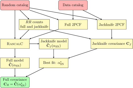
Figure 1: Flowchart of RascalC jackknife pipeline. This process was used for DESI data and most of the mock tests in this paper. In the latter case, a single mock catalog and its corresponding random catalog(s) are provided as data and randoms.

We start by briefly reviewing the methodology developed in [26, 27, 28, 31]. The RascalC code builds single-parameter covariance matrix models based on a random catalog and a table of the 2-point correlation function values. Then we fit a model to the reference covariance to obtain the optimal parameter value for the final prediction. In the fiducial data pipeline, shown schematically in Fig. 1, we measure the correlation function directly from the data, the code produces separate models for full and jackknife covariance matrices, we fit the latter to the data jackknife covariance matrix, and plug the resulting optimal parameter into the full model. In an alternative pipeline (Appendices C and 4), we use the best fit of the full covariance model to the mock sample covariance instead. In the following, we provide more details.

The Landy-Szalay estimator [40] for the 2-point correlation function (2PCF) in radial bin $a$ and angular bin $c$ is

$$\quantity(\hat{\xi}^{XY})_{a}^{c}=\frac{\quantity(N^{X}N^{Y})_{a}^{c}}{\quantity(R^{X}R^{Y})_{a}^{c}}$$ (2.1)

where $N=D-R$, $R$ are random points and $D$ are data points; one can further write

$$\quantity(N^{X}N^{Y})_{a}^{c}=\sum_{i\neq j}n^{X}_{i}n^{Y}_{j}w^{X}_{i}w^{Y}_{j}\Theta^{a}(r_{ij})\Theta^{c}(\mu_{ij})\delta^{X}_{i}\delta^{Y}_{j}.$$ (2.2)

Here a grid of cubic cells has been assigned to the survey such that each cell contains no more than one galaxy, $n^{X}_{i}$ is the expected mean number density of tracer $X$ in the cell $i$, $w_{i}$ is the expected mean weight, $\delta_{i}$ is the fractional galaxy overdensity, $\mu_{ij}$ is the absolute value of the cosine of the angle between the line of sight and the separation vector $\mathbf{r}_{ij}=\mathbf{r}_{i}-\mathbf{r}_{j}$ ($r_{ij}$ being its absolute value), and $\Theta$ are binning functions (unity if the argument fits into the bin and zero otherwise).

Then the covariance matrix can be computed, for convenience designated as

$$\quantity(C^{XY,ZW})_{ab}^{cd}\equiv\operatorname{cov}\quantity[\quantity(\hat{\xi}^{XY})_{a}^{c},\quantity(\hat{\xi}^{ZW})_{b}^{d}].$$ (2.3)

The covariance can be expanded using Eqs. 2.1 and 2.2 and separated into sums over configurations of 4, 3, and 2 points (since some of the four can coincide) [26]. The shot-noise approximation was then used to deal with squares of overdensity:

$$\quantity(\delta^{X}_{i})^{2}\approx\frac{\alpha_{\rm SN}^{X}}{n^{X}_{i}}\quantity(1+\delta^{X}_{i}).$$ (2.4)

It includes a shot-noise rescaling parameter $\alpha_{\rm SN}^{X}$. The “default”, Poissonian shot-noise corresponds to $\alpha_{\rm SN}^{X}=1$, but the parameter can be set to other values for different tracers to improve the realism of the covariance matrix, as detailed below. An intuitive expectation is for $\alpha_{\rm SN}^{X}>1$, since non-Gaussianity typically enhances the small-scale clustering, although it has not been proven strictly.

The resulting expression for single tracer $X$ is

$$\quantity(\tilde{C}^{XX,XX})_{ab}^{cd}\quantity(\alpha_{\rm SN}^{X})=\quantity({}^{4}C^{XX,XX})_{ab}^{cd}+\alpha_{\rm SN}^{X}\quantity({}^{3}C^{X,XX})_{ab}^{cd}+\quantity(\alpha_{\rm SN}^{X})^{2}\quantity({}^{2}C^{XX})_{ab}^{cd},$$ (2.5)

the $d$-point terms ${}^{d}{\bf C}$ are defined in Eq. A.2.

Previous works have established the procedure of taking the Gaussian limit: nulling the 3-point function and the connected 4-point function, and instead adjusting the covariance matrix with shot-noise rescaling parameter(s) $\bm{\alpha}_{\rm SN}$ according to Eq. A.1. This does not remove the 3- and 4-point terms completely, because they have contributions from the 2PCF.

The 4, 3, and 2-point terms (Eq. A.2) are estimated using Monte Carlo importance sampling of points from random catalogs [28]; the RascalC code also requires random counts for normalization and a table of correlation function values to evaluate the summands in Eq. A.2 [31].

The shot-noise rescaling parameter can be optimized to match a sample covariance based on a smaller set of mocks [26] or to jackknife covariance from the data itself [27]. The latter only requires mocks for initial validation (like in this paper), and then allows to generate covariance matrices for different setups more quickly and easily, without the need to generate or adjust simulations for them. We advise the reader to remark that the code does not fit the final covariance to the jackknife one, but makes a separate theoretical prediction for the latter, taking into account the correlations between the jackknife regions.

The code uses a slightly non-standard formalism, dubbed unrestricted jackknife [28]. There the jackknife correlation function estimate $\xi_{A}$ is not the auto-correlation of the whole survey excluding the jackknife region $A$, but the cross-correlation function between that region and the whole survey. Equivalently, this means that the additional jackknife weighting factor for the pair of points $i,j$, $q^{A}_{ij}$, is 1 if both of them belong to the jackknife region $A$, $1/2$ if only one and 0 if neither. Then the pair counts can be converted from different terms (auto and cross jackknife counts) often saved separately in light of Mohammad-Percival correction [24].

The unrestricted jackknife is convenient since the full pair counts of all types are the sum of all the jackknife ones. So if one weighs the regions by the $RR$ pair counts,

$$\quantity(w^{XY}_{A})_{a}^{c}=\frac{\quantity(R^{X}R^{Y}_{A})_{a}^{c}}{\quantity(R^{X}R^{Y})_{a}^{c}},$$ (2.6)

the weighted mean correlation function is equal to the full-survey one.

The data jackknife covariance estimate is then

$$\quantity(C_{J}^{XY,ZW})_{ab}^{cd}=\frac{\sum_{A}\quantity(w^{XY}_{A})_{a}^{c}\quantity(w^{ZW}_{A})_{b}^{d}\quantity[\quantity(\hat{\xi}^{XY}_{A})_{a}^{c}-\quantity(\hat{\xi}^{XY})_{a}^{c}]\quantity[\quantity(\hat{\xi}^{ZW}_{A})_{b}^{d}-\quantity(\hat{\xi}^{ZW})_{b}^{d}]}{1-\sum_{A}\quantity(w^{XY}_{A})_{a}^{c}\quantity(w^{ZW}_{A})_{b}^{d}},$$ (2.7)

the corresponding theoretical estimate, $\quantity(\tilde{C}_{J}^{XY,ZW})_{ab}^{cd}$, is constructed analogously to Eq. A.1 but with different terms defined in Eq. A.3.

Shot-noise rescaling has been obtained for each tracer separately by fitting the prediction for its auto-correlation function’s jackknife covariance (constructed analogously to Eq. 2.5 but with the terms given by Eq. A.3) to the data (Eq. 2.7). More specifically, this involves the minimization of the Kullback-Leibler (KL) divergence, where the RascalC covariance is inverted [28] (since the jackknife one is often not invertible). The final covariance is obtained by plugging the resulting shot-noise rescaling values into Eq. A.1.

Theoretically, inversion of the RascalC covariance gives a slightly biased estimate of the precision matrix. However, the Hartlap factor [18] is not applicable since it is not a sample covariance. The relevant correction matrix accounting for importance sampling noise has been worked out [27], but we find it practically insignificant: the eigenvalues deviate from 1 by $\lesssim 10^{-3}$.

Standard BAO reconstruction procedures shift the positions of both the data $D$ and random points. Original random points $R$ are kept as well, the shifted ones are commonly denoted by $S$. The correlation function is estimated via the Landy-Szalay estimator (Eq. 2.1) with $N=D-S$ instead of $D-R$. As [31] argued, in the computations of covariance matrices for reconstructed catalogs we used the shifted randoms $S$ in the importance sampling, not shifted random counts for normalization in Eqs. A.2 and A.3 and slightly differently normalized two-point correlation function for the integrands:

$$\quantity(\hat{\xi}^{XY}_{\rm in})_{a}^{c}=\frac{\quantity(N^{X}N^{Y})_{a}^{c}}{\quantity(S^{X}S^{Y})_{a}^{c}}.$$ (2.8)

To summarise, the main approximation is that shot-noise rescaling of purely Gaussian contributions (i.e., ignoring 3-point and connected 4-point function, only based on 2-point) can produce a realistic covariance matrix in configuration space. A theoretical motivation for this is that non-Gaussian contributions primarily affect the squeezed configurations involving small-scale correlations, below the bin width for the 2-point function, while the shot noise regulates infinitesimally small scales. The method has been empirically shown to agree well enough with the mock-based covariances [26, 41, 31] so far.

2.2 Comparison measures for covariance matrices

We employ the same three compact measures of covariance matrix similarity as in RascalC validation for early DESI data [31]. We use RascalC precision (inverse covariance) matrix ${\bf\Psi}_{R}={\bf C}_{R}^{-1}$ and the mock sample covariance matrix ${\bf C}_{S}$ because the latter is more noisy and thus less stable to inversion. We also find this ordering more interpretable: some additional properties do not hold with the other one, as noted below.

1. Kullback-Leibler divergence

   $$D_{\rm KL}\quantity({\bf\Psi}_{R},{\bf C}_{S})=\frac{1}{2}\quantity[\tr({\bf\Psi}_{R}{\bf C}_{S})-N_{\rm bins}-\ln\det({\bf\Psi}_{R}{\bf C}_{S})],$$ (2.9)

   which is used to optimize shot-noise rescaling, and related to the log-likelihood of the sample covariance under the assumption that the RascalC covariance is truly describing the distribution of mock clustering measurements [26].

2. The directional RMS relative difference:

   $$R_{\rm inv}\quantity({\bf\Psi}_{R},{\bf C}_{S})=\frac{1}{\sqrt{N_{\rm bins}}}\norm{{\bf C}_{S}^{1/2}{\bf\Psi}_{R}{\bf C}_{S}^{1/2}-{\bf\mathbb{I}}}_{F}=\sqrt{\frac{\tr[\quantity({\bf\Psi}_{R}{\bf C}_{S}-{\bf\mathbb{I}})^{2}]}{N_{\rm bins}}}.$$ (2.10)

3. The mean reduced chi-squared:

   $$\chi^{2}_{\rm red}\quantity({\bf\Psi}_{R},{\bf C}_{S})=\frac{1}{N_{\rm bins}}\tr({\bf\Psi}_{R}{\bf C}_{S}),$$ (2.11)

   which is distributed like a reduced $\chi^{2}$ with $N_{\rm bins}\times(n_{S}-1)$ degrees of freedom under the assumption that RascalC covariance describes the distribution of the mock clustering measurements.

The first two are sensitive to deviations in different ways, but their expectation values would not be zero even if RascalC covariance matrices perfectly matched the true underlying covariance. The last measure, mean reduced $\chi^{2}$, is more sensitive to the overall scaling between the covariance matrices, while deviations in different directions can cancel each other.

The expectation values and standard deviations for all the measures have been derived in [31]; the result for $\chi^{2}_{\rm red}$ is exact while the other two are approximate. We have performed empirical validations using 10,000 samples with a unit covariance matrix and the desired number of bins. We have found significant deviations for KL divergence in observable space (due to more multipoles and thus total bins considered in this paper) and smaller ones for $R_{\rm inv}$ in parameter space; in these cases, we reverted to the empirical means and standard deviations.

2.3 Fisher projection to the space of model parameters

As in [31], we approximate the covariance matrices in the parameter space through the inverse of the Fisher matrix. For RascalC results, we a simple expression without inversion bias corrections (which are small for our semi-analytical covariance matrices):

$${\bf C}_{R}^{\rm par}=\quantity[{\bf M}\quantity({\bf C^{\prime}}^{\rm obs}_{R})^{-1}{\bf M}^{T}]^{-1}.$$ (2.12)

${\bf C^{\prime}}^{\rm obs}_{R}$ is the observable-space RascalC covariance matrix cut to the fit range for the respective model encompassing $N^{\prime}_{\rm bins}$ observables, and ${\bf M}$ is the Jacobian of the model, specifically the matrix of derivatives of the vector of radially-binned 2PCF multipoles $\bm{\xi}$ with respect to the parameter vector $\bm{\theta}$:

$$M_{ra}\equiv\frac{\partial\xi_{a}}{\partial\theta_{r}}.$$ (2.13)

For the mock sample covariance, we use

$${\bf C}_{S}^{\rm par}=\frac{n_{S}-1}{n_{S}-N^{\prime}_{\rm bins}+N_{\rm pars}-1}\quantity[{\bf M}\quantity({\bf C^{\prime}}^{\rm obs}_{S})^{-1}{\bf M}^{T}]^{-1},$$ (2.14)

which is analogous to Eq. 2.12, only with a leading-order bias correction coefficient accounting for both matrix inversions, per Eq. (B6) of [42].

3 Covariance for projected Legendre moments of 2PCF revisited

Because of the great advantage of using few estimators and hence a smaller covariance matrix, multipole moments are a compression favorable to many angular bins. A past RascalC extension introduced the estimators for their covariance, assuming weighting by Legendre polynomials during pair counting, or infinitesimally narrow angular bins [29]. At the same time, the 2-point correlation function estimation library widely used in DESI, pycorr, estimates the radially binned Legendre moments of the 2-point correlation function from the radially and angularly binned estimates $\quantity(\hat{\xi}^{XY})_{a}^{c}$ (Eq. 2.1) with $\sim 100$ angular bins (after wrapping):

$$\quantity(\hat{\xi}^{XY})^{\ell}_{a} =\quantity(2\ell+1)\sum_{c}\quantity(\xi^{XY})_{a}^{c}\int_{\Delta\mu_{c}}d\mu\,L_{\ell}(\mu)=\sum_{c}\quantity(\xi^{XY})_{a}^{c}F^{\ell}_{c};$$ (3.1)

$$F^{\ell}_{c} \equiv\quantity(2\ell+1)\int_{\Delta\mu_{c}}d\mu\,L_{\ell}\quantity(\mu)$$ (3.2)

are the projection factors, which do not depend on radial bins or the tracers involved in the correlation function. The equations above assume even multipole index $\ell$ and wrapping of the binned pair counts to $\mu\in[0,1]$.

The difference between the infinite and large finite numbers of $\mu$ bins is not a major accuracy issue. However, the previous methodology for Legendre moments had other practical disadvantages: it required a separate jackknife computation for $r,\mu$ bins just to tune the shot-noise rescaling, and a fit for the survey correction function — the ratio of pair counts in a real survey and an idealized one (similar to a periodic box with the same volume) – for which a piecewise-polynomial form was used somewhat arbitrarily [29]. We have seen this mismatch as an opportunity to streamline the covariance matrix computation procedure for extensive usage with DESI.

Since the projection in Eq. 3.1 is linear, the covariance matrix for these Legendre moments estimators can be obtained from the $r,\mu$-binned one given by Eq. A.1:

$$\quantity(\tilde{C}^{XY,ZW})_{ab}^{pq}=\sum_{c,d}\quantity(\tilde{C}^{XY,ZW})_{ab}^{cd}F^{p}_{c}F^{q}_{d}.$$ (3.3)

A major technical result of this paper is to present a methodology to accumulate this covariance matrix of the Legendre multipoles directly within the summation over point configurations, rather than having to compute and then project the much larger covariance matrix of fine angular bins. For this, several quantities need to be inserted into the sums of Eq. A.2, and we obtain the following 4, 3, and 2-point terms:

$$\quantity({}^{4}C^{XY,ZW})_{ab}^{pq} =\sum_{i\neq j\neq k\neq l}n^{X}_{i}n^{Y}_{j}n^{Z}_{k}n^{W}_{l}w^{X}_{i}w^{Y}_{j}w^{Z}_{k}w^{W}_{l}\Theta^{a}(r_{ij})\Theta^{b}(r_{kl})$$ (3.4)

$$\times\quantity[\cancel{\eta^{({\rm c}),XYWZ}_{ijkl}}+2\xi^{XZ}_{ik}\xi^{YW}_{jl}]\sum_{c}\frac{\Theta^{c}(\mu_{ij})F^{p}_{c}}{\quantity(R^{X}R^{Y})_{a}^{c}}\sum_{d}\frac{\Theta^{d}(\mu_{kl})F^{q}_{d}}{\quantity(R^{Z}R^{W})_{b}^{d}},$$

$$\quantity({}^{3}C^{Y,XZ})_{ab}^{pq} =4\sum_{i\neq j\neq k}n^{X}_{i}n^{Y}_{j}n^{Z}_{k}w^{X}_{i}\quantity(w^{Y}_{j})^{2}w^{Z}_{k}\Theta^{a}(r_{ij})\Theta^{b}(r_{jk})\quantity[\cancel{\zeta^{XYZ}_{ijk}}+\xi^{XZ}_{ik}]$$

$$\times\sum_{c}\frac{\Theta^{c}(\mu_{ij})F^{p}_{c}}{\quantity(R^{X}R^{Y})_{a}^{c}}\sum_{d}\frac{\Theta^{d}(\mu_{jk})F^{q}_{d}}{\quantity(R^{Y}R^{Z})_{b}^{d}},$$

$$\quantity({}^{2}C^{XY})_{ab}^{pq} =2\delta^{ab}\sum_{i\neq j}n^{X}_{i}n^{Y}_{j}\quantity(w^{X}_{i}w^{Y}_{j})^{2}\Theta^{a}(r_{ij})\quantity[1+\xi^{XY}_{ij}]\sum_{c}\frac{\Theta^{c}(\mu_{ij})F^{p}_{c}F^{q}_{c}}{\quantity[\quantity(R^{X}R^{Y})_{a}^{c}]^{2}}.$$

Like in Eq. A.2, we include the non-Gaussian higher-point function but null them in the current implementation, which is marked by crossing them out. Sums like $\sum_{c}\Theta^{c}(\mu)\dots$ practically mean finding the angular bin $\tilde{c}$ to which the $\mu$ value belongs and then evaluating the rest only for that one bin. Within the code, we sample a quad, triple, or pair of particles and then accumulate its contribution to all the Legendre multipole moments in its radial bin.

These 4, 3, and 2-point terms can be combined to the full theoretical estimate via

$$\quantity(C^{XY,ZW})_{ab}^{pq}=\quantity({}^{4}C^{XY,ZW})_{ab}^{pq}+\frac{\alpha_{\rm SN}^{X}}{4}\quantity[\delta^{XW}\quantity({}^{3}C^{X,YZ})_{ab}^{pq}+\delta^{XZ}\quantity({}^{3}C^{X,YW})_{ab}^{pq}]$$ (3.5)

$$+\frac{\alpha_{\rm SN}^{Y}}{4}\quantity[\delta^{YW}\quantity({}^{3}C^{Y,XZ})_{ab}^{pq}+\delta^{YZ}\quantity({}^{3}C^{Y,XW})_{ab}^{pq}]$$

$$+\frac{\alpha_{\rm SN}^{X}\alpha_{\rm SN}^{Y}}{2}\quantity(\delta^{XW}\delta^{YZ}+\delta^{XZ}\delta^{YW})\quantity({}^{2}C^{XY})_{ab}^{pq}.$$

The next sections of this paper only deal with single-tracer covariances, but we provide them since they have been used for cross-correlation analysis [35].

We have found it challenging to design a reasonable and convenient weighting for the jackknife estimates of the Legendre multipole moments. Instead, we have decided to project the $r,\mu$-binned jackknife covariance matrix estimate (Eq. (2.7)) similarly to the full covariance (Eq. (3.3)):

$$\quantity(C^{XY,ZW}_{J})_{ab}^{pq}=\sum_{c,d}\quantity(C^{XY,ZW}_{J})_{ab}^{cd}F^{p}_{c}F^{q}_{d}$$ (3.6)

and project the theoretical predictions (Eq. (A.3)) in the same fashion, for the just comparison:

$$\quantity(\tilde{C}_{J}^{XY,ZW})_{ab}^{pq}=\quantity({}^{4}C_{J}^{XY,ZW})_{ab}^{pq}+\frac{\alpha_{\rm SN}^{X}}{4}\quantity[\delta^{XW}\quantity({}^{3}C_{J}^{X,YZ})_{ab}^{pq}+\delta^{XZ}\quantity({}^{3}C_{J}^{X,YW})_{ab}^{pq}]$$ (3.7)

$$+\frac{\alpha_{\rm SN}^{Y}}{4}\quantity[\delta^{YW}\quantity({}^{3}C_{J}^{Y,XZ})_{ab}^{pq}+\delta^{YZ}\quantity({}^{3}C_{J}^{Y,XW})_{ab}^{pq}]$$

$$+\frac{\alpha_{\rm SN}^{X}\alpha_{\rm SN}^{Y}}{2}\quantity[\delta^{XW}\delta^{YZ}+\delta^{XZ}\delta^{YW}]\quantity({}^{2}C_{J}^{XY})_{ab}^{pq}$$

with

$$\quantity({}^{4}C_{J}^{XY,ZW})_{ab}^{pq} =\sum_{i\neq j\neq k\neq l}n^{X}_{i}n^{Y}_{j}n^{Z}_{k}n^{W}_{l}w^{X}_{i}w^{Y}_{j}w^{Z}_{k}w^{W}_{l}\Theta^{a}(r_{ij})\Theta^{b}(r_{kl})$$ (3.8)

$$\times\quantity[\cancel{\eta^{({\rm c}),XYWZ}_{ijkl}}+\xi^{XY}_{ij}\xi^{ZW}_{kl}+2\xi^{XZ}_{ik}\xi^{YW}_{jl}]$$

$$\times\sum_{c,d}\frac{\quantity(\omega^{XY,ZW}_{ijkl})_{ab}^{cd}\Theta^{c}(\mu_{ij})\Theta^{d}(\mu_{kl})F^{p}_{c}F^{q}_{d}}{\quantity(R^{X}R^{Y})_{a}^{c}\quantity(R^{Z}R^{W})_{b}^{d}\quantity[1-\sum_{A}\quantity(w^{XY}_{A})_{a}^{c}\quantity(w^{ZW}_{A})_{b}^{d}]},$$

$$\quantity({}^{3}C_{J}^{Y,XZ})_{ab}^{pq} =4\sum_{i\neq j\neq k}n^{X}_{i}n^{Y}_{j}n^{Z}_{k}w^{X}_{i}\quantity(w^{Y}_{j})^{2}w^{Z}_{k}\Theta^{a}(r_{ij})\Theta^{b}(r_{jk})\quantity[\cancel{\zeta^{XYZ}_{ijk}}+\xi^{XZ}_{ik}]$$

$$\times\sum_{c,d}\frac{\quantity(\omega^{XY,YZ}_{ijjk})_{ab}^{cd}\Theta^{c}(\mu_{ij})\Theta^{d}(\mu_{jk})F^{p}_{c}F^{q}_{d}}{\quantity(R^{X}R^{Y})_{a}^{c}\quantity(R^{Y}R^{Z})_{b}^{d}\quantity[1-\sum_{A}\quantity(w^{XY}_{A})_{a}^{c}\quantity(w^{YZ}_{A})_{b}^{d}]},$$

$$\quantity({}^{2}C_{J}^{XY})_{ab}^{pq} =2\delta^{ab}\sum_{i\neq j}n^{X}_{i}n^{Y}_{j}\quantity(w^{X}_{i}w^{Y}_{j})^{2}\Theta^{a}(r_{ij})\quantity[1+\xi^{XY}_{ij}]$$

$$\times\sum_{c}\frac{\quantity(\omega^{XY,XY}_{ijij})_{ab}^{cc}\Theta^{c}(\mu_{ij})F^{p}_{c}F^{q}_{c}}{\quantity[\quantity(R^{X}R^{Y})_{a}^{c}]^{2}\quantity{1-\sum_{A}\quantity[\quantity(w^{XY}_{A})_{a}^{c}]^{2}}}.$$

Similarly, sums of the form $\sum_{c,d}\Theta^{c}(\mu_{1})\Theta^{d}(\mu_{2})\dots$ practically mean finding the angular bins $\tilde{c},\tilde{d}$ to which the $\mu_{1,2}$ values belong correspondingly and then evaluating the rest only for that pair of bins. In practice, in the 4-point term, we also omit the disconnected part ($\xi^{XY}_{ij}\xi^{ZW}_{kl}$), since it complicates the computation and has been found very small in practice.

The key advantage of this new mode is making the Legendre covariance with shot-noise rescaling tuned on jackknives in one go, instead of having to perform two separate runs previously. Additionally, one does not need to fit the survey correction function with a somewhat arbitrary form in non-trivial geometry [29]; instead, the random-random counts are used directly.

4 Validation setup

In this section, we describe how we validate these methods and the RascalC code on applications for DESI. To do so, we apply the data pipeline (Fig. 1) to single mock catalogs, as was done in previous works. This implies using the random files, full and jackknife correlation function estimates specific to that catalog. Similarly to [31], we use effective Zel’dovich (EZ) mocks [13, 14], apply compact covariance matrix similarity measures to each of the single-mock runs before and after standard BAO reconstruction (pre- and post-recon) in the observable space (i.e., in terms of correlation function multipoles), and then also project the covariances into the model parameter space (as described in Section 2.3). Earlier papers [27, 28, 29] did not use the full set of the compact similarity measures, did not provide both their expectation values and standard deviations for the perfect theoretical covariance case (Section 2.2) and did not project to parameter space(s). Relative to [31], the new features of this work are:

• including quadrupole and hexadecapole moments of the correlation function with the new method (Section 3);

• mocks run through fast fiber assignment [43], which mimics the fiber assignment effects on the real survey [44];

• including more tracers (galaxy types): not only luminous red galaxies (LRG) [45] ($z=0.8-1.1$ bin in this work), but also emission line galaxies (ELG) [46] $z=1.1-1.6$ and magnitude-limited bright galaxy survey (BGS) [47] $z=0.1-0.4$, corresponding to LRG3, ELG2 and BGS samples in the main BAO paper [7] respectively, as summarized in Table 1;

• comparing different separation ranges and sets of multipoles in the observable space (not only the widest one, Section 5.3);

• considering more models for Fisher projections: instead of only 1D (isotropic) BAO, now we have 2D BAO, ShapeFit and direct fit (Section 5.4);

• as for the data, the covariances have been run separately for North and South galactic caps (NGC and SGC) and then combined as a weighted average assuming those regions are uncorrelated (Appendix B).

Tracer	LRG	ELG	BGS
$z$ range	$(0.8,1.1)$	$(1.1,1.6)$	$(0.1,0.4)$
Designation in [6, 7]	LRG3	ELG2	BGS
EZmocks snapshot $z$	1.1	1.325	0.2

Table 1: Tracers and redshift bins used in this paper. For LRG and ELG, which have multiple bins unlike BGS, we have selected the densest ones, as shot-noise seems easier to capture with RascalC. We did not include the quasars (QSO) for the same reason. The snapshot redshifts were used to construct the power spectrum templates.

To set up the covariances (Fig. 1), we have used 10 mocks for each of the 3 tracers, pre- and post-recon, and 6 different cuts or projections. The mock sample covariance was computed with all 1000 EZmocks in each case. We have decided to only present the mean and standard deviation of the comparison measures across the 10 mocks, the full set of numbers will be available in the supplementary material.

We use the suite of EZmocks calibrated to the clustering of the DESI One-percent survey data [4], cut to the DESI DR1 footprint [15] and run through fast fiber assignment [43].

Effects of fiber assignment may pose additional challenges to the method because it involves anisotropic pair-wise sampling, depending both on the density of the targets and the number of survey passes in the region [44]. We provide the RascalC code with the random catalog and clustering estimate affected by fiber assignment (see the flowchart in Fig. 1), but the expansion leading to Eq. A.2 (and Eq. A.3) uses the survey-wide correlation function(s) to calculate the ensemble averages of products of overdensities, and the shot-noise rescaling (Eq. 2.4) is also global. It is challenging to let them vary without complicating the covariance matrix model too much and introducing too many parameters.

Fiber assignment incompleteness might also cause issues with jackknife. Ideally, one would like each sub-region to have a distribution of the number of passes representative of the full survey. This is challenging to achieve, and the jackknife assignment based on data $K$-means clustering (implemented in pycorr and used in this work) likely does not guarantee that.

We have not endeavored to validate multi-tracer covariances in this work because the snapshot redshifts for most overlapping tracers do not match in the EZmocks suite. The main interest has been in the LRG and ELG overlap in $z=0.8-1.1$ bin [35], but the snapshot redshifts are 1.1 and 0.95 respectively. We expect that the shift of the positions with time will not allow self-consistent cross-correlations. Only part of the QSO come from snapshot redshift 1.1, but that overlap will be even less significant than with ELG.

The reconstruction procedure follows the findings of the DESI DR1 optimal reconstruction task force [33, 34]: the RecSym mode of the IterativeFFTReconstruction algorithm [48] from the pyrecon package with smoothing scale of $15\,h^{-1}{\rm Mpc}$.

The covariance matrices have been created for monopole, quadrupole and hexadecapole in 45 radial bins between 20 and 200 $h^{-1}{\rm Mpc}$ (each 4 $h^{-1}{\rm Mpc}$ wide). We have excluded the $s<20\,h^{-1}{\rm Mpc}$ bins because they impede the convergence of the covariance matrices, and also because we expect the shot-noise rescaling to become inadequate on small scales.

We also project the covariance matrices into parameter spaces of models according to Section 2.3. We used the following ones implemented in the desilike package:

• 2D BAO – BAO power spectrum template and polynomial-based broadband modeling (as detailed in [7]), fit to monopole and quadrupole in radial bins spanning $s=48-152\,h^{-1}{\rm Mpc}$;

• Full-shape fits using monopole, quadrupole and hexadecapole in radial bins spanning $s=28-152\,h^{-1}{\rm Mpc}$ and relying on the velocileptors Lagrangian perturbation theory model [49, 50, 51] with maximum freedom, standard prior basis and different power spectrum templates:

  • ShapeFit: a compression method using parametric variations of a single power spectrum template evaluated at the reference cosmology and introducing parametric variations [52];

  • Direct fit: linear power spectrum from the CLASS Boltzmann code [53].

Unlike in [31], we exclude the nuisance parameters right away by leaving out the corresponding rows and columns from the covariance matrices given by Eqs. 2.14 and 2.12. The remaining sub-matrix represents the covariance of the parameters of interest marginalized over the others. The RascalC precision matrix is then simply the inverse of this restricted covariance (as the inversion bias is practically negligible for semi-analytical results).

We used a fixed model Jacobian (Eq. 2.13): computed once at the best fit to the mean clustering of all the available mocks (using the mock sample covariance matrix) for each case (tracer, pre- or post-recon, and the model). This is a limitation, which nevertheless allowed us to summarize the comparison measures for all the 10 tested mocks for each setup, and keep the perfect reference simpler.

We also refer the reader to the companion covariance comparison paper [32] for thorough plots of the fit results (not only errorbar estimates, but also parameters’ best values) for each mock catalog with the mock sample covariance against those with RascalC ones. On the flip side, such a detailed approach limited the number of RascalC realizations that could be presented.

5 Results

Having described the methodology for the current RascalC validation on EZmocks in the previous section, we proceed to detail the results of its application.

5.1 Runtime and intrinsic convergence checks

As in [31], we begin by using $R_{\rm inv}$ between the different estimates of each RascalC covariance matrix from separate halves of the Monte-Carlo integration samples for an additional quality assessment before looking at the sample covariance matrices.

We found that the LRG covariance matrices each reached $R_{\rm inv}\leq 2.0\%$ convergence within 4 node-hours on the NERSC Perlmutter supercomputer. The ELG covariance matrices reached $R_{\rm inv}\leq 2.9\%$ convergence within 10 node-hours, while those of BGS reached $R_{\rm inv}<11.5\%$ convergence within 12 node-hours. A single Perlmutter node has a CPU with 128 cores with 256 hyperthreads, all of which are utilized by RascalC. In a few cases, the result was considerably worse, then additional runs were performed, and used either instead or together with the first runs, depending on their $R_{\rm inv}$.

Relative to [31], these are longer runtimes and yet less converged $R_{\rm inv}$ (the maximum was $0.63\%$ back then). We believe the key reason is a larger number of observables in the covariance matrix (3 times more – the same number of radial bins, but now 3 multipoles instead of 1). For reference, the comparison of a sample covariance based on 1000 realizations with the true covariance matrix describing the samples’ distribution yields $R_{\rm inv}\approx 37\%$ (Table 4). Moreover, the tracers with a higher number density (ELG and especially BGS) are more challenging due to the increasing importance of the 4-point term relative to the 3- and 2-point terms. The more points, the more configurations need to be sampled for good precision of the term.

5.2 Shot-noise rescaling values

$\alpha_{\rm SN}$	NGC		SGC
	Mocks	Data	Mocks	Data
LRG pre-recon	$0.743\pm 0.012$	0.86	$0.7935\pm 0.0081$	0.95
LRG post-recon	$0.770\pm 0.010$	0.85	$0.809\pm 0.011$	0.96
ELG pre-recon	$0.3757\pm 0.0043$	0.68	$0.4018\pm 0.0014$	0.72
ELG post-recon	$0.3789\pm 0.0044$	0.69	$0.4051\pm 0.0044$	0.74
BGS pre-recon	$0.792\pm 0.012$	0.85	$0.8198\pm 0.0091$	0.88
BGS post-recon	$0.812\pm 0.012$	0.87	$0.8447\pm 0.0095$	0.92

Table 2: Shot-noise rescaling values for mocks and data.

$\alpha_{\rm SN}$	North	South
LRG pre-recon	0.97	0.99
LRG post-recon	0.98	1.00
BGS pre-recon	1.03	0.96
BGS post-recon	0.96	1.02

Table 3: Shot-noise rescaling values for Early DESI data [30] (a two-month subset of the DR1). Note that the redshift ranges were different from the current ones (Table 1): BGS $z=0.1-0.5$, LRG $z=0.4-1.1$.

As we pointed out in Section 2.1, our method uses a rescaling of the shot noise contribution to account for differences between the true small-scale contributions and our Gaussian approximation. After reaching a relatively uniform convergence level, we inspect the shot-noise rescaling values obtained from fitting the jackknife covariances in Table 2. Interestingly, we find that all the shot-noise rescaling values are smaller than 1, i.e., that the jackknife variations are smaller than predicted by Gaussian approximation with standard Poisson shot-noise (Eq. 2.4). This is different from what has been found in previous mock studies [26, 27, 28, 31], but we believe that this is a consequence of the effects of fiber assignment incompleteness. In contrast, the results for the early DESI data [30], which had more uniform completeness, showed shot-noise rescaling values close to 1, as shown in Table 3.

Next, we see that the shot-noise rescaling values are significantly lower on mocks compared to the data. Again, the difference is most pronounced for ELG. This is an indication that the fast fiber assignment does not exactly reproduce the covariance matrix/shot-noise properties of the real one.

In light of the concerns about fiber assignment and jackknife discussed in Section 4, these results warrant further investigation. We have come up with a self-consistency test for our covariance matrix models: optimization of the shot-noise rescaling based on mock sample covariance (detailed in Appendix C and particularly Fig. 4). We show the resulting values along with the baseline, jackknife-based ones in Table 10, and find them very close for all cases. In other words, calibration of shot-noise rescaling on jackknives still brings us close to an optimal fit on the mocks. With that, we have decided to proceed further with the validation process. This will show how close this nearly optimal fit is to the mock sample covariance.

5.3 Observable space

	$D_{\rm KL}({\bf\Psi}_{R},{\bf C}_{S})$	$R_{\rm inv}({\bf\Psi}_{R},{\bf C}_{S})$	$\chi^{2}_{\rm red}({\bf\Psi}_{R},{\bf C}_{S})$
Perfect	$4.817\pm 0.070$	$0.3690\pm 0.0031$	$1.0000\pm 0.0039$
LRG pre-recon	$4.856\pm 0.029$	$0.3678\pm 0.0049$	$0.989\pm 0.016$
	($0.55\pm 0.41$)$\sigma$	($-0.4\pm 1.6$)$\sigma$	($-2.7\pm 4.1$)$\sigma$
LRG post-recon	$4.977\pm 0.050$	$0.3581\pm 0.0034$	$0.957\pm 0.014$
	($2.27\pm 0.70$)$\sigma$	($-3.5\pm 1.1$)$\sigma$	($-11.3\pm 3.6$)$\sigma$
ELG pre-recon	$4.811\pm 0.024$	$0.3700\pm 0.0055$	$1.000\pm 0.015$
	($-0.09\pm 0.34$)$\sigma$	($0.3\pm 1.8$)$\sigma$	($0.1\pm 3.8$)$\sigma$
ELG post-recon	$5.001\pm 0.018$	$0.3701\pm 0.0042$	$0.986\pm 0.012$
	($2.61\pm 0.26$)$\sigma$	($0.4\pm 1.4$)$\sigma$	($-3.6\pm 3.1$)$\sigma$
BGS pre-recon	$5.129\pm 0.052$	$0.3824\pm 0.0081$	$0.997\pm 0.016$
	($4.43\pm 0.73$)$\sigma$	($4.4\pm 2.6$)$\sigma$	($-0.8\pm 4.2$)$\sigma$
BGS post-recon	$5.177\pm 0.077$	$0.3810\pm 0.0079$	$0.994\pm 0.016$
	($5.1\pm 1.1$)$\sigma$	($3.9\pm 2.6$)$\sigma$	($-1.4\pm 4.1$)$\sigma$

Table 4: Summary of full measurement-space comparison of RascalC covariances with the sample covariances (135 bins, $s=20-200~{}h^{-1}{\rm Mpc}$, monopole, quadrupole and hexadecapole).

We now begin to compare the RascalC results with the mock sample covariance matrices. We start in Table 4 with the widest available range: $s=20-200~{}h^{-1}{\rm Mpc}$ using all three multipoles. We remind that for a fixed tracer pre- or post-recon, all 10 single-mock results are compared to the same sample covariance matrix, so that noise, which is accounted for in the “perfect case” is “fixed” independently from mock-to-mock scatter in RascalC results. Ideally, we would like the comparison measures to be within the perfect reference ranges for the majority of them. We can see this is not always the case. We remind that the first two measures accumulate deviations in all “directions”. The KL divergences approach 3 sigma high level for LRG and ELG post-recon, while for BGS they are even further from perfect. $R_{\rm inv}$ are high with a larger scatter for BGS. In the reduced chi-squared, which captures the overall “scaling” with higher accuracy, the mean values for the RascalC runs are shifted significantly for LRG and ELG post-recon, and the mock-to-mock scatter is high in all the cases.

	$D_{\rm KL}({\bf\Psi}_{R},{\bf C}_{S})$	$R_{\rm inv}({\bf\Psi}_{R},{\bf C}_{S})$	$\chi^{2}_{\rm red}({\bf\Psi}_{R},{\bf C}_{S})$
Perfect	$2.260\pm 0.049$	$0.3067\pm 0.0036$	$1.0000\pm 0.0046$
LRG pre-recon	$2.307\pm 0.022$	$0.3056\pm 0.0037$	$0.983\pm 0.016$
	($0.99\pm 0.46$)$\sigma$	($-0.3\pm 1.0$)$\sigma$	($-3.7\pm 3.4$)$\sigma$
LRG post-recon	$2.333\pm 0.027$	$0.2998\pm 0.0024$	$0.960\pm 0.014$
	($1.52\pm 0.56$)$\sigma$	($-1.93\pm 0.68$)$\sigma$	($-8.7\pm 3.0$)$\sigma$
ELG pre-recon	$2.2578\pm 0.0095$	$0.3050\pm 0.0044$	$0.995\pm 0.014$
	($-0.04\pm 0.20$)$\sigma$	($-0.5\pm 1.2$)$\sigma$	($-1.0\pm 3.1$)$\sigma$
ELG post-recon	$2.292\pm 0.013$	$0.3044\pm 0.0033$	$0.987\pm 0.012$
	($0.67\pm 0.28$)$\sigma$	($-0.65\pm 0.93$)$\sigma$	($-2.8\pm 2.6$)$\sigma$
BGS pre-recon	$2.414\pm 0.025$	$0.3140\pm 0.0066$	$0.987\pm 0.016$
	($3.18\pm 0.52$)$\sigma$	($2.0\pm 1.9$)$\sigma$	($-2.7\pm 3.4$)$\sigma$
BGS post-recon	$2.479\pm 0.038$	$0.3202\pm 0.0065$	$0.993\pm 0.016$
	($4.52\pm 0.78$)$\sigma$	($3.8\pm 1.8$)$\sigma$	($-1.5\pm 3.4$)$\sigma$

Table 5: Summary of measurement-space comparison of RascalC covariances with the sample covariances restricted to the range of ShapeFit and direct fits (93 bins, $s=28-152~{}h^{-1}{\rm Mpc}$, monopole, quadrupole and hexadecapole).

We continue the comparisons in Table 5, now cutting the range to $s=28-152~{}h^{-1}{\rm Mpc}$ as is common for full-shape fits (ShapeFit and direct). The KL divergences and $R_{\rm inv}$ become more consistent with the perfect reference cases for LRG and ELG, but remain high for BGS. The scaling difference (in reduced chi-squared) remains similar.

	$D_{\rm KL}({\bf\Psi}_{R},{\bf C}_{S})$	$R_{\rm inv}({\bf\Psi}_{R},{\bf C}_{S})$	$\chi^{2}_{\rm red}({\bf\Psi}_{R},{\bf C}_{S})$
Perfect	$0.702\pm 0.027$	$0.2303\pm 0.0046$	$1.0000\pm 0.0062$
LRG pre-recon	$0.763\pm 0.014$	$0.2351\pm 0.0023$	$0.982\pm 0.016$
	($2.29\pm 0.54$)$\sigma$	($1.04\pm 0.49$)$\sigma$	($-2.9\pm 2.6$)$\sigma$
LRG post-recon	$0.732\pm 0.013$	$0.2281\pm 0.0019$	$0.964\pm 0.015$
	($1.14\pm 0.50$)$\sigma$	($-0.48\pm 0.40$)$\sigma$	($-5.7\pm 2.3$)$\sigma$
ELG pre-recon	$0.7195\pm 0.0083$	$0.2317\pm 0.0039$	$0.999\pm 0.015$
	($0.65\pm 0.31$)$\sigma$	($0.30\pm 0.86$)$\sigma$	($-0.2\pm 2.4$)$\sigma$
ELG post-recon	$0.6903\pm 0.0088$	$0.2278\pm 0.0029$	$0.995\pm 0.012$
	($-0.45\pm 0.33$)$\sigma$	($-0.54\pm 0.62$)$\sigma$	($-0.8\pm 1.9$)$\sigma$
BGS pre-recon	$0.796\pm 0.021$	$0.2419\pm 0.0079$	$0.982\pm 0.018$
	($3.54\pm 0.78$)$\sigma$	($2.5\pm 1.7$)$\sigma$	($-2.8\pm 2.8$)$\sigma$
BGS post-recon	$0.777\pm 0.031$	$0.2462\pm 0.0090$	$1.011\pm 0.017$
	($2.8\pm 1.2$)$\sigma$	($3.4\pm 1.9$)$\sigma$	($1.8\pm 2.7$)$\sigma$

Table 6: Summary of measurement-space comparison of RascalC covariances with the sample covariances restricted to the range of BAO fits (52 bins, $s=48-152~{}h^{-1}{\rm Mpc}$, monopole and quadrupole).

We perform the final set of observable-space comparisons in Table 6, further restricting the range to $s=48-152~{}h^{-1}{\rm Mpc}$ and using only monopole and quadrupole, without hexadecapole. We do not see significant consistency changes from the previous case.

We note that the abovementioned differences are relatively small — in the reduced chi-squared at most $(4.3\pm 1.4)\%$ for LRG post-recon in the widest range, and in $R_{\rm inv}$ – no more than a percent or two on top of $23-37\%$ caused by the finite sample size. We should ask whether we trust the realism of the mocks to that level in all aspects of the correlation function multipoles. Moreover, for the real survey matching the clustering between data and simulations will become an additional issue for mocks. We remind that here we are running RascalC with clustering measured directly with each respective mock.

5.4 Model parameter spaces

Now we proceed to project the covariance matrices to model parameters (as described in Section 2.3).

5.4.1 BAO

	$D_{\rm KL}({\bf\Psi}_{R},{\bf C}_{S})$	$R_{\rm inv}({\bf\Psi}_{R},{\bf C}_{S})$	$\chi^{2}_{\rm red}({\bf\Psi}_{R},{\bf C}_{S})$
Perfect	$0.0015\pm 0.0012$	$0.051\pm 0.021$	$1.000\pm 0.032$
LRG pre-recon	$0.00219\pm 0.00081$	$0.064\pm 0.012$	$0.940\pm 0.012$
	($0.56\pm 0.66$)$\sigma$	($0.61\pm 0.54$)$\sigma$	($-1.91\pm 0.39$)$\sigma$
LRG post-recon	$0.00220\pm 0.00051$	$0.0639\pm 0.0071$	$0.9481\pm 0.0095$
	($0.56\pm 0.41$)$\sigma$	($0.63\pm 0.34$)$\sigma$	($-1.64\pm 0.30$)$\sigma$
ELG pre-recon	$0.00043\pm 0.00024$	$0.0284\pm 0.0090$	$1.023\pm 0.011$
	($-0.87\pm 0.20$)$\sigma$	($-1.04\pm 0.42$)$\sigma$	($0.71\pm 0.34$)$\sigma$
ELG post-recon	$0.00091\pm 0.00043$	$0.041\pm 0.010$	$0.964\pm 0.012$
	($-0.48\pm 0.35$)$\sigma$	($-0.46\pm 0.47$)$\sigma$	($-1.15\pm 0.39$)$\sigma$
BGS pre-recon	$0.0049\pm 0.0014$	$0.095\pm 0.013$	$0.913\pm 0.013$
	($2.8\pm 1.2$)$\sigma$	($2.06\pm 0.59$)$\sigma$	($-2.76\pm 0.42$)$\sigma$
BGS post-recon	$0.00032\pm 0.00012$	$0.0251\pm 0.0049$	$1.0112\pm 0.0091$
	($-0.960\pm 0.095$)$\sigma$	($-1.20\pm 0.23$)$\sigma$	($0.35\pm 0.29$)$\sigma$

Table 7: Summary of parameter-space comparison of RascalC covariances with the sample covariances projected to the BAO fit parameters, ${\alpha_{\rm iso}}$ and ${\alpha_{\rm AP}}$.

In Table 7 we compare the covariances projected to the BAO parameters, the scales ${\alpha_{\rm iso}}$ and ${\alpha_{\rm AP}}$. The comparison measures look consistent with the perfect reference case. The most significant deviations are seen in BGS pre-recon: both the KL divergence and $R_{\rm inv}$ are high, while the reduced chi-squared is almost 3 sigma low on average (meaning that the RascalC covariance is “larger” than the mock sample one). The mock-to-mock scatter in RascalC results is always lower than the noise expected from the finite mock sample size.

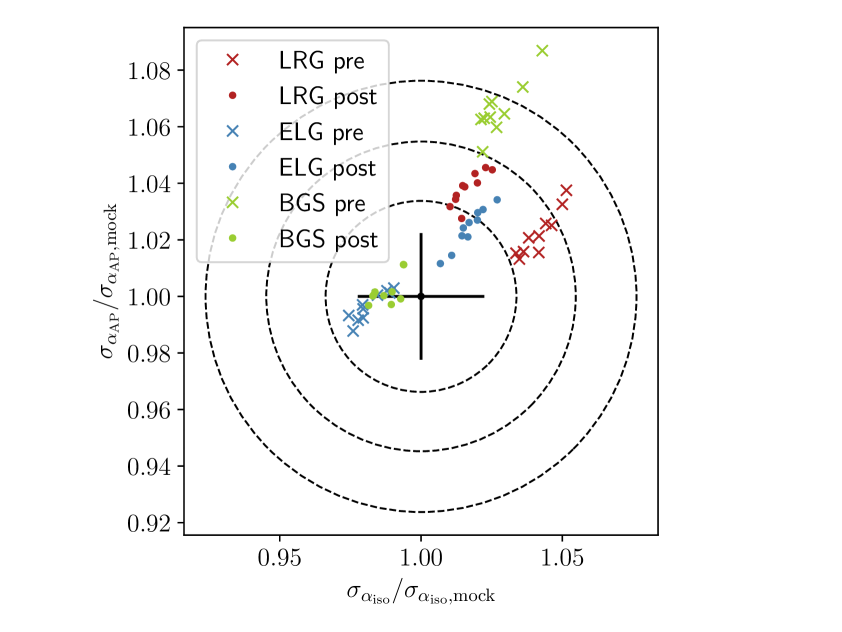
Figure 2: Comparison of the projected errorbars for the BAO scale parameters, normalized to the values obtained from the mock sample covariance. The cross shows one-dimensional relative precisions ($\quantity(2\quantity(n_{S}-1))^{-1/2}\approx 2.2\%$ [31]) following from the EZmocks sample size ($n_{S}=1000$), and the dashed ellipses approximately correspond to two-dimensional 68%, 95% and 99.7% confidence regions in this 2D space of errorbars. Here the correlation of errorbars is ignored; it varies in different cases but is too small to notice ($\lesssim 0.04$).

We have also plotted the errorbars on ${\alpha_{\rm iso}}$ and ${\alpha_{\rm AP}}$ against each other in Fig. 2. They corroborate with Table 7: most deviations are within the 99.7% contour, except a few of the BGS pre-recon runs. However, remember that these plots do not show the covariance of the parameters, which is taken into account with KL divergence and $R_{\rm inv}$.

5.4.2 Full shape: ShapeFit and direct fit

	$D_{\rm KL}({\bf\Psi}_{R},{\bf C}_{S})$	$R_{\rm inv}({\bf\Psi}_{R},{\bf C}_{S})$	$\chi^{2}_{\rm red}({\bf\Psi}_{R},{\bf C}_{S})$
Perfect	$0.0050\pm 0.0023$	$0.069\pm 0.016$	$1.000\pm 0.022$
LRG pre-recon	$0.0059\pm 0.0023$	$0.073\pm 0.013$	$0.969\pm 0.020$
	($0.4\pm 1.0$)$\sigma$	($0.25\pm 0.81$)$\sigma$	($-1.39\pm 0.89$)$\sigma$
LRG post-recon	$0.00739\pm 0.00087$	$0.0840\pm 0.0052$	$0.984\pm 0.022$
	($1.06\pm 0.39$)$\sigma$	($0.95\pm 0.33$)$\sigma$	($-0.73\pm 0.98$)$\sigma$
ELG pre-recon	$0.0063\pm 0.0029$	$0.078\pm 0.015$	$1.005\pm 0.027$
	($0.6\pm 1.3$)$\sigma$	($0.59\pm 0.94$)$\sigma$	($0.2\pm 1.2$)$\sigma$
ELG post-recon	$0.0029\pm 0.0013$	$0.052\pm 0.011$	$0.999\pm 0.017$
	($-0.95\pm 0.58$)$\sigma$	($-1.06\pm 0.68$)$\sigma$	($-0.06\pm 0.78$)$\sigma$
BGS pre-recon	$0.0071\pm 0.0030$	$0.083\pm 0.019$	$0.996\pm 0.031$
	($0.9\pm 1.3$)$\sigma$	($0.9\pm 1.2$)$\sigma$	($-0.2\pm 1.4$)$\sigma$
BGS post-recon	$0.0067\pm 0.0027$	$0.080\pm 0.017$	$0.992\pm 0.030$
	($0.7\pm 1.2$)$\sigma$	($0.7\pm 1.1$)$\sigma$	($-0.3\pm 1.3$)$\sigma$

Table 8: Summary of parameter-space comparison of RascalC covariances with the sample covariances projected to the ShapeFit parameters: ${\alpha_{\rm iso}}$, ${\alpha_{\rm AP}}$, $dm$ and $df$.

Table 8 shows the comparison measures for the covariances projected to the ShapeFit parameters: ${\alpha_{\rm iso}}$, ${\alpha_{\rm AP}}$, $dm$ and $df$. We do not see significant statistical deviations from the perfect case. This is the only case when BGS (both pre- and post-recon) are not particularly far from the reference. The mock-to-mock scatter in RascalC results is smaller than or comparable with the noise in the sample covariances.

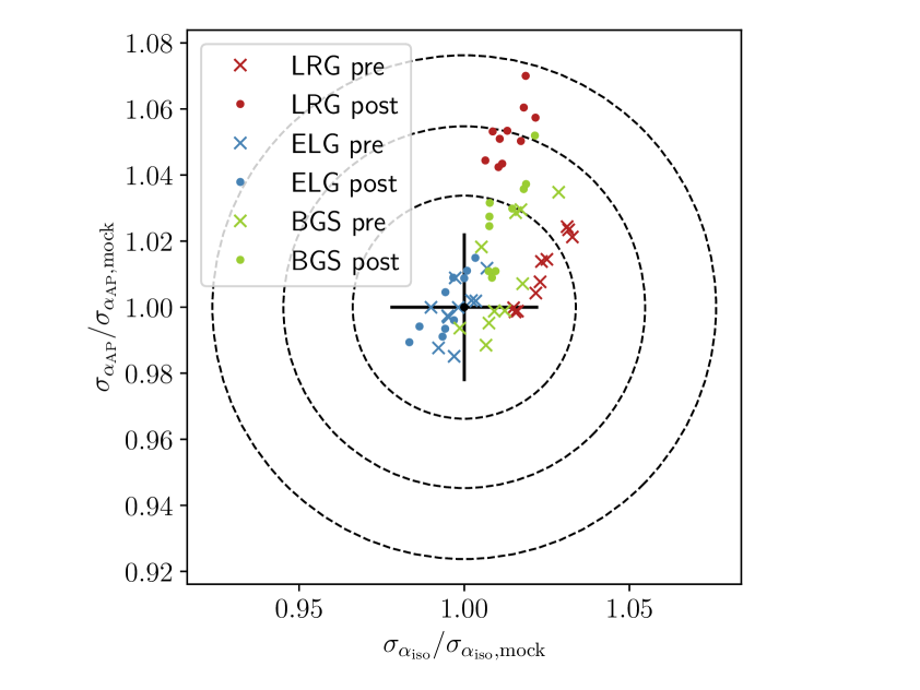
Figure 3: Same as Fig. 2 but with errorbars for the scale parameters following from ShapeFit.

Additionally, in Fig. 3 we compare the projected errorbars for the scale parameters, ${\alpha_{\rm iso}}$ and ${\alpha_{\rm AP}}$. All the points fall within the 99.7% confidence region in this 2D space, although the other parameters and cross-correlations are ignored in this picture, unlike in Table 8.

	$D_{\rm KL}({\bf\Psi}_{R},{\bf C}_{S})$	$R_{\rm inv}({\bf\Psi}_{R},{\bf C}_{S})$	$\chi^{2}_{\rm red}({\bf\Psi}_{R},{\bf C}_{S})$
Perfect	$0.0050\pm 0.0023$	$0.069\pm 0.016$	$1.000\pm 0.022$
LRG pre-recon	$0.0099\pm 0.0034$	$0.093\pm 0.014$	$0.951\pm 0.020$
	($2.2\pm 1.5$)$\sigma$	($1.50\pm 0.89$)$\sigma$	($-2.20\pm 0.91$)$\sigma$
LRG post-recon	$0.00360\pm 0.00068$	$0.0584\pm 0.0055$	$0.976\pm 0.016$
	($-0.63\pm 0.30$)$\sigma$	($-0.66\pm 0.35$)$\sigma$	($-1.08\pm 0.71$)$\sigma$
ELG pre-recon	$0.0061\pm 0.0013$	$0.0783\pm 0.0094$	$1.013\pm 0.024$
	($0.48\pm 0.60$)$\sigma$	($0.59\pm 0.59$)$\sigma$	($0.6\pm 1.1$)$\sigma$
ELG post-recon	$0.0033\pm 0.0014$	$0.055\pm 0.011$	$0.985\pm 0.016$
	($-0.75\pm 0.60$)$\sigma$	($-0.85\pm 0.72$)$\sigma$	($-0.68\pm 0.72$)$\sigma$
BGS pre-recon	$0.0101\pm 0.0073$	$0.099\pm 0.040$	$1.013\pm 0.035$
	($2.3\pm 3.2$)$\sigma$	($1.9\pm 2.5$)$\sigma$	($0.6\pm 1.5$)$\sigma$
BGS post-recon	$0.0083\pm 0.0045$	$0.090\pm 0.027$	$1.003\pm 0.035$
	($1.5\pm 2.0$)$\sigma$	($1.3\pm 1.7$)$\sigma$	($0.1\pm 1.5$)$\sigma$

Table 9: Summary of parameter-space comparison of RascalC covariances with the sample covariances projected to the direct fit parameters: $h$, $\omega_{\rm cdm}$, $\omega_{b}$ and $\log A_{s}$.

Finally, in Table 9 we provide the comparison results for the covariances projected to the direct fit parameters, $h$, $\omega_{\rm cdm}$, $\omega_{b}$ and $\log A_{s}$. We see deviations exceeding 3 sigma in most of the measures for LRG pre-recon and of BGS; LRG post-recon and ELG look consistent.

Still, the differences we see are at a few percent level, and the limitations of the realism of the mocks might be responsible for them.

6 Conclusions

We have presented and validated the DESI DR1 pipeline for the semi-analytical covariance matrices of the galaxy 2-point correlation functions on realistic mock catalogs.

We have developed a streamlined procedure for the estimation of the semi-analytical covariance matrices for Legendre moments of the 2PCF in separation bins with the RascalC code [28]. The previous implementation [29] required an additional computation with angular bins to mimic the non-Gaussian effects by calibrating the shot-noise rescaling value on the jackknife covariance matrix estimate. Now this calibration can be achieved with one run of the code. This allowed for more efficient massive production of covariance matrices for all the tracers, redshift bins, and galactic caps of DESI DR1 galaxies and quasars data.

We have applied this updated pipeline to an isolated mock catalog with fast (approximate) fiber assignment, representative of DESI DR1, 10 times for 3 selected tracers and redshift bins (LRG3, ELG2 and BGS according to [7]), without and with standard BAO reconstruction applied.

First, we note the difference between the shot-noise rescaling values obtained for the mocks with fast fiber assignment and the data in Section 5.2. However, the parameter calibration on jackknife and mock sample covariance yields very close results in the mock runs (Appendix C). Therefore, this indicates that the fast fiber assignment likely does not reproduce all the properties of the real one relevant to the covariance matrix properties.

Then, we apply the set of compact measures of covariance matrix similarity from [31] in the observable space (correlation function multipoles) in Section 5.3, as well as projected linearly (through Fisher matrix formalism) to the parameters of different models in Section 5.4. We find some deviations that can not be explained solely by the finite sample size limiting the accuracy of the mock-based covariance. However, they are at a few percent level. We argue that our goal is not necessarily to match the mocks perfectly, given their unavoidably approximate nature (including the fast fiber assignment mentioned above). One should also remember that the mocks have a disadvantage when it comes to calibration to the data clustering, especially with blinding.

Since the key application of RascalC covariance matrices at the moment is to the DESI DR1 baryon acoustic oscillations analysis [7], the results projected for the BAO model (Section 5.4.1) are of particular importance. There, for the errorbars of the scale parameters, ${\alpha_{\rm iso}}$ and ${\alpha_{\rm AP}}$, we find a close agreement ($\leq 5\%$, while the standard deviation of the errorbar expected from 1000 mock samples is $\approx 2.4\%$), except for BGS before reconstruction.

The covariance matrices for the BGS sample are found to be less consistent in most of the comparisons (except in ShapeFit parameters). We expected them to be more challenging to RascalC because of higher number density and thus higher significance of the 4-point term compared to the 3- and 2-point terms. This already caused slower convergence and could further demonstrate the limitations of the shot-noise rescaling. However, BGS have been challenging for the EZmocks as well, so their sample covariance is likely to be a less robust reference than for LRG and ELG.

The observable-space results (Section 5.3) may leave an impression that RascalC performance worsened with fiber assignment. However, the previous RascalC validation for early DESI data [31] used an earlier version of EZmocks without fast fiber assignment. Before focusing on the isotropic BAO scales, the covariance matrices there also showed statistically significant variations from the sample covariance, although they were deemed acceptable as comparable to the scatter in semi-analytical results; in this work we use a stricter interpretation, testing whether every RascalC single-mock result is consistent with the perfect-case reference. In future work, we could repeat the tests on the mocks before fiber assignment with all the tracers (and multipoles) used in this paper.

Another direction for further improvement is to study the dependence of shot-noise rescaling on fiber assignment incompleteness by running RascalC on survey sub-regions with a more uniform number of passes. It is also possible that a prescription for higher-point non-Gaussian correlations with a low number of parameters would give a better consistency with the reference than rescaling the covariance matrix terms in which they are nulled. However, for such precision studies, it is instructive to have extremely reliable, realistic and numerous mocks.

Extensions of the approach beyond the standard 2-point function are possible but require extra work. For example, [29] introduced the covariance matrices for isotropic 3-point correlation functions.

In summary, we have validated RascalC semi-analytical covariance matrices for 2PCF as a very viable alternative to the mock-based ones. Despite the increase in the runtime of the RascalC code (from 50-150 to 500-1500 core-hours, or 4-12 node-hours at NERSC Perlmutter supercomputer, Section 5.1), the method is far faster than calibrating, generating, and processing a suite of mocks numerous enough to give an adequate covariance matrix precision. We have shown that the two methods produce similar results given the requirements of the DESI 2024 BAO analysis. The speed advantage of the semi-analytic method permits easier exploration of situations where one cannot afford to regenerate mock catalogs, such as different assumptions about cosmology, galaxy-halo connection, or non-standard sample selections. We therefore expect that such semi-analytic methods can be of broad utility for computing large-scale covariance matrices in wide-field surveys.

Data availability

The data used in this analysis will be made public along with the DESI Data Release 1 (details in https://data.desi.lbl.gov/doc/releases/). The code used in the paper is publicly available at https://github.com/oliverphilcox/RascalC and https://github.com/misharash/RascalC-scripts. The data from the plots, the full set of computed comparison measures and shot-noise rescaling values are available at doi:10.5281/zenodo.10895161 [54].

Appendix A Details on previous covariance estimators

A.1 Full

The full multi-tracer expression for the model covariance (not used in this work, but employed for overlapping tracers’ cross-correlation in [35]) is

$$\quantity(\tilde{C}^{XY,ZW})_{ab}^{cd}\quantity(\bm{\alpha}_{\rm SN})=\quantity({}^{4}C^{XY,ZW})_{ab}^{cd}+\frac{\alpha_{\rm SN}^{X}}{4}\quantity[\delta^{XW}\quantity({}^{3}C^{X,YZ})_{ab}^{cd}+\delta^{XZ}\quantity({}^{3}C^{X,YW})_{ab}^{cd}]$$ (A.1)

$$+\frac{\alpha_{\rm SN}^{Y}}{4}\quantity[\delta^{YW}\quantity({}^{3}C^{Y,XZ})_{ab}^{cd}+\delta^{YZ}\quantity({}^{3}C^{Y,XW})_{ab}^{cd}]$$

$$+\frac{\alpha_{\rm SN}^{X}\alpha_{\rm SN}^{Y}}{2}\quantity[\delta^{XW}\delta^{YZ}+\delta^{XZ}\delta^{YW}]\quantity({}^{2}C^{XY})_{ab}^{cd}$$

with

$$\quantity({}^{4}C^{XY,ZW})_{ab}^{cd} =\frac{1}{\quantity(R^{X}R^{Y})_{a}^{c}\quantity(R^{Z}R^{W})_{b}^{d}}\sum_{i\neq j\neq k\neq l}n^{X}_{i}n^{Y}_{j}n^{Z}_{k}n^{W}_{l}w^{X}_{i}w^{Y}_{j}w^{Z}_{k}w^{W}_{l}\Theta^{a}(r_{ij})$$ (A.2)

$$\times\Theta^{c}(\mu_{ij})\Theta^{b}(r_{kl})\Theta^{d}(\mu_{kl})\quantity[\cancel{\eta^{({\rm c}),XYWZ}_{ijkl}}+\xi^{XZ}_{ik}\xi^{YW}_{jl}+\xi^{XW}_{il}\xi^{YZ}_{jk}]$$

$$\quantity({}^{3}C^{Y,XZ})_{ab}^{cd} =\frac{4}{\quantity(R^{X}R^{Y})_{a}^{c}\quantity(R^{Y}R^{Z})_{b}^{d}}\sum_{i\neq j\neq k}n^{X}_{i}n^{Y}_{j}n^{Z}_{k}w^{X}_{i}\quantity(w^{Y}_{j})^{2}w^{Z}_{k}\Theta^{a}(r_{ij})\Theta^{c}(\mu_{ij})$$

$$\times\Theta^{b}(r_{jk})\Theta^{d}(\mu_{jk})\quantity[\cancel{\zeta^{XYZ}_{ijk}}+\xi^{XZ}_{ik}]$$

$$\quantity({}^{2}C^{XY})_{ab}^{cd} =\frac{2\delta^{ab}\delta^{cd}}{\quantity(R^{X}R^{Y})_{a}^{c}\quantity(R^{X}R^{Y})_{b}^{d}}\sum_{i\neq j}n^{X}_{i}n^{Y}_{j}\quantity(w^{X}_{i}w^{Y}_{j})^{2}\Theta^{a}(r_{ij})\Theta^{c}(\mu_{ij})\quantity[1+\xi^{XY}_{ij}],$$

where $\delta^{XY}$, $\delta^{ab}$ and $\delta^{cd}$ are Kronecker deltas; $\xi^{XY}_{ij}=\xi^{XY}\quantity(r_{ij},\mu_{ij})$ is the 2PCF of tracers $X$ and $Y$ evaluated at the separation between points number $i$ and $j$ (in practice the value is obtained by bicubic interpolation from the input grid of correlation function values).

Analogously, $\zeta^{XYZ}_{ijk}$ and $\eta^{{(\rm c)},XYZW}_{ijkl}$ are the 3-point and connected 4-point correlation functions of the tracers listed in the superscript evaluated at the separations between $i,j,k$ and $i,j,k,l$ points, respectively. These non-Gaussian higher-point functions are included for completeness but nulled in practice, we reflected this by crossing them out in the expressions.

A.2 Jackknife

The full multi-tracer jackknife covariance model can be constructed analogously to Eq. A.1 but with the following terms:

$$\quantity({}^{4}C_{J}^{XY,ZW})_{ab}^{cd} =\frac{1}{\quantity(R^{X}R^{Y})_{a}^{c}\quantity(R^{Z}R^{W})_{b}^{d}\quantity[1-\sum_{A}\quantity(w^{XY}_{A})_{a}^{c}\quantity(w^{ZW}_{A})_{b}^{d}]}$$ (A.3)

$$\times\sum_{i\neq j\neq k\neq l}n^{X}_{i}n^{Y}_{j}n^{Z}_{k}n^{W}_{l}w^{X}_{i}w^{Y}_{j}w^{Z}_{k}w^{W}_{l}\Theta^{a}(r_{ij})\Theta^{c}(\mu_{ij})\Theta^{b}(r_{kl})\Theta^{d}(\mu_{kl})$$

$$\times\quantity[\cancel{\eta^{({\rm c}),XYWZ}_{ijkl}}+\xi^{XY}_{ij}\xi^{ZW}_{kl}+2\xi^{XZ}_{ik}\xi^{YW}_{jl}]\quantity(\omega^{XY,ZW}_{ijkl})_{ab}^{cd}$$

$$\quantity({}^{3}C_{J}^{Y,XZ})_{ab}^{cd} =\frac{4}{\quantity(R^{X}R^{Y})_{a}^{c}\quantity(R^{Y}R^{Z})_{b}^{d}\quantity[1-\sum_{A}\quantity(w^{XY}_{A})_{a}^{c}\quantity(w^{YZ}_{A})_{b}^{d}]}$$

$$\times\sum_{i\neq j\neq k}n^{X}_{i}n^{Y}_{j}n^{Z}_{k}w^{X}_{i}\quantity(w^{Y}_{j})^{2}w^{Z}_{k}\Theta^{a}(r_{ij})\Theta^{c}(\mu_{ij})\Theta^{b}(r_{jk})\Theta^{d}(\mu_{jk})$$

$$\times\quantity[\cancel{\zeta^{XYZ}_{ijk}}+\xi^{XZ}_{ik}]\quantity(\omega^{XY,YZ}_{ijjk})_{ab}^{cd}$$

$$\quantity({}^{2}C_{J}^{XY})_{ab}^{cd} =\frac{2\delta^{ab}\delta^{cd}}{\quantity(R^{X}R^{Y})_{a}^{c}\quantity(R^{X}R^{Y})_{b}^{d}\quantity[1-\sum_{A}\quantity(w^{XY}_{A})_{a}^{c}\quantity(w^{XY}_{A})_{b}^{d}]}$$

$$\times\sum_{i\neq j}n^{X}_{i}n^{Y}_{j}\quantity(w^{X}_{i}w^{Y}_{j})^{2}\Theta^{a}(r_{ij})\Theta^{c}(\mu_{ij})\quantity[1+\xi^{XY}_{ij}]\quantity(\omega^{XY,XY}_{ijij})_{ab}^{cd},$$

where $\quantity(\omega_{ijkl})_{ab}^{cd}$ is an additional jackknife weight tensor:

$$\quantity(\omega^{XY,ZW}_{ijkl})_{ab}^{cd}=\sum_{A}\quantity[q^{A}_{ij}-\quantity(w^{XY}_{A})_{a}^{c}]\quantity[q^{A}_{kl}-\quantity(w^{ZW}_{A})_{b}^{d}].$$ (A.4)

Appendix B Covariance for the combination of two regions

B.1 Angular bins

In pycorr, during the combination of regions labeled by $G$, the total counts $QQ$ (where each $Q$ can be $D$ or $R$, data or randoms) become

$$\quantity(Q^{X}Q^{Y})_{a}^{c}=\sum_{G}\quantity(Q^{X}Q^{Y}_{G})_{a}^{c}.$$ (B.1)

Prior to that, all the counts are brought to the same normalization within each region, which does not affect the correlation function. The norms for the total counts of each type are sums of the corresponding norms for the two regions. So they are also the same for all total counts. Therefore, in all these cases, the correlation function is equal to the ratio of non-normalized counts, not only the normalized ones. Then the total correlation function is simply the average weighted by $RR$ counts:

$$\quantity(\xi^{XY})_{a}^{c} =\frac{1}{\quantity(R^{X}R^{Y})_{a}^{c}}\sum_{G}\quantity(R^{X}R^{Y}_{G})_{a}^{c}\quantity(\xi^{XY}_{G})_{a}^{c}\equiv\sum_{G}\quantity(W^{XY}_{G})_{a}^{c}\quantity(\xi^{XY}_{G})_{a}^{c},$$ (B.2)

$$\quantity(W^{XY}_{G})_{a}^{c} \equiv\frac{\quantity(R^{X}R^{Y}_{G})_{a}^{c}}{\quantity(R^{X}R^{Y})_{a}^{c}}.$$ (B.3)

Then the covariance matrix for the combined region is simply

$$\quantity(C^{XY,ZW})_{ab}^{cd}\approx\sum_{G}\quantity(C^{XY,ZW}_{G})_{ab}^{cd}\quantity(W^{XY}_{G})_{a}^{c}\quantity(W^{ZW}_{G})_{b}^{d},$$ (B.4)

where we neglect the covariance between the correlation functions in different regions, the estimation of which poses extra challenges. For the North and South Galactic caps in the DESI footprint, which are well separated from each other, this seems like a safe approximation.

B.2 Legendre

We can build upon the results for angular bins, with conversions both ways between them and Legendre moments. The Legendre multipoles are estimated from the angular bins via Eqs. 3.1 and 3.2:

$$\quantity(\xi^{XY})^{\ell}_{a}=\sum_{c}\quantity(\xi^{XY})_{a}^{c}F^{\ell}_{c}.$$ (B.5)

One can do the reverse approximately with bin-averaged values of the Legendre polynomials:

$$L_{\ell}^{c} \equiv\frac{1}{\Delta\mu_{c}}\int_{\Delta\mu_{c}}d\mu\,L_{\ell}(\mu)=\frac{F^{\ell}_{c}}{(2\ell+1)\Delta\mu_{c}},$$ (B.6)

$$\quantity(\xi^{XY})_{a}^{c} \approx\sum_{\ell}\quantity(\hat{\xi}^{XY})^{\ell}_{a}L_{\ell}^{c}.$$ (B.7)

These do not depend on the region, and work equally well for the combined one as for parts. Additional approximation comes from the fact that we limit the multipole index — in this work we only consider $\ell=0,2,4$.

So we can work out the partial derivative of the Legendre moment of the combined correlation function with respect to one in each of the regions in the following steps:

$$\frac{\partial\quantity(\xi^{XY})^{p}_{a}}{\partial\quantity(\xi^{XY}_{G})^{q}_{a}}=\sum_{c}\frac{\partial\quantity(\xi^{XY})^{p}_{a}}{\partial\quantity(\xi^{XY})^{c}_{a}}\frac{\partial\quantity(\xi^{XY})^{c}_{a}}{\partial\quantity(\xi^{XY}_{G})^{c}_{a}}\frac{\partial\quantity(\xi^{XY}_{G})^{c}_{a}}{\partial\quantity(\xi^{XY}_{G})^{q}_{a}}\approx\sum_{c}F_{c}^{p}\quantity(W^{XY}_{G})_{a}^{c}L^{c}_{q}\equiv\quantity(W_{G}^{XY})^{p,q}_{a};$$ (B.8)

the different separation bins and correlation functions stay independent.

Then the covariance matrix for the combined region’s 2PCF is

$$\quantity(C^{XY,ZW})_{ab}^{pq}\approx\sum_{G}\sum_{p^{\prime},q^{\prime}}\quantity(C^{XY,ZW}_{G})_{ab}^{p^{\prime}q^{\prime}}\quantity(W^{XY}_{G})_{a}^{p,p^{\prime}}\quantity(W^{ZW}_{G})_{b}^{q,q^{\prime}},$$ (B.9)

here we also neglect the covariance between the correlation functions in different regions.

Appendix C Shot-noise rescaling based on mocks

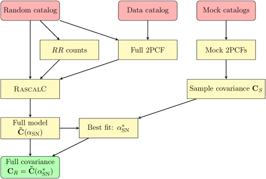
Figure 4: Flowchart of RascalC mocks pipeline. This process was only used for some tests on mocks, in which data is substituted by a single mock catalog. The full covariance model can be reused from a jackknife run (Fig. 1), provided that the randoms and full 2PCF were the same.

We show the procedure for fitting the shot-noise rescaling to the mock sample covariance schematically in Fig. 4. It is similar to the method of [26], used before utilizing jackknife was proposed in [27]. The resulting RascalC covariance matrix is the best fit (in terms of KL divergence) of the full covariance model to the mock sample covariance matrix; this procedure can be seen as theoretically motivated smoothing.

$\alpha_{\rm SN}$	NGC		SGC
	Jackknife	Mock sample	Jackknife	Mock sample
LRG pre	$0.743\pm 0.012$	$0.7417\pm 0.0038$	$0.7935\pm 0.0081$	$0.7906\pm 0.0045$
LRG post	$0.770\pm 0.010$	$0.7446\pm 0.0029$	$0.809\pm 0.011$	$0.7945\pm 0.0032$
ELG pre	$0.3757\pm 0.0043$	$0.3757\pm 0.0013$	$0.4018\pm 0.0014$	$0.4077\pm 0.0016$
ELG post	$0.3789\pm 0.0044$	$0.3751\pm 0.0013$	$0.4051\pm 0.0044$	$0.4067\pm 0.0017$
BGS pre	$0.792\pm 0.012$	$0.7916\pm 0.0068$	$0.8198\pm 0.0091$	$0.827\pm 0.014$
BGS post	$0.812\pm 0.012$	$0.8148\pm 0.0070$	$0.8447\pm 0.0095$	$0.844\pm 0.013$

Table 10: Shot-noise rescaling values for the single-mock runs calibrated on jackknife (Fig. 1) and mock sample covariances (Fig. 4).

We show the shot-noise rescaling values obtained from jackknife (the main method) and mock sample covariance in Table 10. The numbers are very close in all cases. The deviations from the mean are not highly correlated mock-to-mock, but this can be expected due to additional scatter in individual jackknife covariances – the mock sample covariance used for reference was based on all 1000 mocks and thus the same for 10 single-mock runs for each case.

Appendix D Author affiliations

¹Center for Astrophysics $|$ Harvard & Smithsonian, 60 Garden Street, Cambridge, MA 02138, USA

²Institute of Physics, Laboratory of Astrophysics, École Polytechnique Fédérale de Lausanne (EPFL), Observatoire de Sauverny, CH-1290 Versoix, Switzerland

³IRFU, CEA, Université Paris-Saclay, F-91191 Gif-sur-Yvette, France

⁴Physics Department, Yale University, P.O. Box 208120, New Haven, CT 06511, USA

⁵Department of Physics & Astronomy, Ohio University, Athens, OH 45701, USA

⁶Center for Cosmology and AstroParticle Physics, The Ohio State University, 191 West Woodruff Avenue, Columbus, OH 43210, USA

⁷Department of Astronomy, The Ohio State University, 4055 McPherson Laboratory, 140 W 18th Avenue, Columbus, OH 43210, USA

⁸Lawrence Berkeley National Laboratory, 1 Cyclotron Road, Berkeley, CA 94720, USA

⁹Physics Dept., Boston University, 590 Commonwealth Avenue, Boston, MA 02215, USA

¹⁰University of Michigan, Ann Arbor, MI 48109, USA

¹¹Leinweber Center for Theoretical Physics, University of Michigan, 450 Church Street, Ann Arbor, Michigan 48109-1040, USA

¹²Department of Physics & Astronomy, University College London, Gower Street, London, WC1E 6BT, UK

¹³Institute for Computational Cosmology, Department of Physics, Durham University, South Road, Durham DH1 3LE, UK

¹⁴Instituto de Física, Universidad Nacional Autónoma de México, Cd. de México C.P. 04510, México

¹⁵Department of Astronomy, School of Physics and Astronomy, Shanghai Jiao Tong University, Shanghai 200240, China

¹⁶Kavli Institute for Particle Astrophysics and Cosmology, Stanford University, Menlo Park, CA 94305, USA

¹⁷SLAC National Accelerator Laboratory, Menlo Park, CA 94305, USA

¹⁸University of California, Berkeley, 110 Sproul Hall #5800 Berkeley, CA 94720, USA

¹⁹Institut de Física d’Altes Energies (IFAE), The Barcelona Institute of Science and Technology, Campus UAB, 08193 Bellaterra Barcelona, Spain

²⁰Departamento de Física, Universidad de los Andes, Cra. 1 No. 18A-10, Edificio Ip, CP 111711, Bogotá, Colombia

²¹Observatorio Astronómico, Universidad de los Andes, Cra. 1 No. 18A-10, Edificio H, CP 111711 Bogotá, Colombia

²²Department of Physics, The University of Texas at Dallas, Richardson, TX 75080, USA

²³Departament de Física Quàntica i Astrofísica, Universitat de Barcelona, Martí i Franquès 1, E08028 Barcelona, Spain

²⁴Institut d’Estudis Espacials de Catalunya (IEEC), 08034 Barcelona, Spain

²⁵Institut de Ciències del Cosmos (ICCUB), Universitat de Barcelona (UB), c. Martí i Franquès, 1, 08028 Barcelona, Spain.

²⁶Consejo Nacional de Ciencia y Tecnología, Av. Insurgentes Sur 1582. Colonia Crédito Constructor, Del. Benito Juárez C.P. 03940, México D.F. México

²⁷Departamento de Física, Universidad de Guanajuato - DCI, C.P. 37150, Leon, Guanajuato, México

²⁸Fermi National Accelerator Laboratory, PO Box 500, Batavia, IL 60510, USA

²⁹Department of Physics, The Ohio State University, 191 West Woodruff Avenue, Columbus, OH 43210, USA

³⁰School of Mathematics and Physics, University of Queensland, 4072, Australia

³¹NSF NOIRLab, 950 N. Cherry Ave., Tucson, AZ 85719, USA

³²Sorbonne Université, CNRS/IN2P3, Laboratoire de Physique Nucléaire et de Hautes Energies (LPNHE), FR-75005 Paris, France

³³Departament de Física, Serra Húnter, Universitat Autònoma de Barcelona, 08193 Bellaterra (Barcelona), Spain

³⁴Laboratoire de Physique Subatomique et de Cosmologie, 53 Avenue des Martyrs, 38000 Grenoble, France

³⁵Institució Catalana de Recerca i Estudis Avançats, Passeig de Lluís Companys, 23, 08010 Barcelona, Spain

³⁶Department of Physics and Astronomy, University of Sussex, Brighton BN1 9QH, U.K

³⁷Department of Physics & Astronomy, University of Wyoming, 1000 E. University, Dept. 3905, Laramie, WY 82071, USA

³⁸National Astronomical Observatories, Chinese Academy of Sciences, A20 Datun Rd., Chaoyang District, Beijing, 100012, P.R. China

³⁹Instituto Avanzado de Cosmología A. C., San Marcos 11 - Atenas 202. Magdalena Contreras, 10720. Ciudad de México, México

⁴⁰Department of Physics and Astronomy, University of Waterloo, 200 University Ave W, Waterloo, ON N2L 3G1, Canada

⁴¹Waterloo Centre for Astrophysics, University of Waterloo, 200 University Ave W, Waterloo, ON N2L 3G1, Canada

⁴²Perimeter Institute for Theoretical Physics, 31 Caroline St. North, Waterloo, ON N2L 2Y5, Canada

⁴³Space Sciences Laboratory, University of California, Berkeley, 7 Gauss Way, Berkeley, CA 94720, USA

⁴⁴Max Planck Institute for Extraterrestrial Physics, Gießenbachstraße 1, 85748 Garching, Germany

⁴⁵Department of Physics, Kansas State University, 116 Cardwell Hall, Manhattan, KS 66506, USA

⁴⁶Department of Physics and Astronomy, Sejong University, Seoul, 143-747, Korea

⁴⁷Centre for Astrophysics & Supercomputing, Swinburne University of Technology, P.O. Box 218, Hawthorn, VIC 3122, Australia

⁴⁸CIEMAT, Avenida Complutense 40, E-28040 Madrid, Spain

⁴⁹Department of Physics, University of Michigan, Ann Arbor, MI 48109, USA

⁵⁰Department of Astronomy, Tsinghua University, 30 Shuangqing Road, Haidian District, Beijing, China, 100190

References

- [1] DESI Collaboration, A. Aghamousa, J. Aguilar, S. Ahlen, S. Alam, L.E. Allen et al., The DESI Experiment Part I: Science,Targeting, and Survey Design, arXiv e-prints (2016) arXiv:1611.00036 [1611.00036].
- [2] DESI Collaboration, B. Abareshi, J. Aguilar, S. Ahlen, S. Alam, D.M. Alexander et al., Overview of the Instrumentation for the Dark Energy Spectroscopic Instrument, AJ 164 (2022) 207 [2205.10939].
- [3] DESI Collaboration, A.G. Adame, J. Aguilar, S. Ahlen, S. Alam, G. Aldering et al., Validation of the Scientific Program for the Dark Energy Spectroscopic Instrument, AJ 167 (2024) 62 [2306.06307].
- [4] DESI Collaboration, A.G. Adame, J. Aguilar, S. Ahlen, S. Alam, G. Aldering et al., The Early Data Release of the Dark Energy Spectroscopic Instrument, arXiv e-prints (2023) arXiv:2306.06308 [2306.06308].
- [5] DESI Collaboration, DESI 2024 I: Data Release 1 of the Dark Energy Spectroscopic Instrument, in preparation (2024) .
- [6] DESI Collaboration, DESI 2024 II: Sample definitions, characteristics and two-point clustering statistics, in preparation (2024) .
- [7] DESI Collaboration, A.G. Adame, J. Aguilar, S. Ahlen, S. Alam, D.M. Alexander et al., DESI 2024 III: Baryon Acoustic Oscillations from Galaxies and Quasars, arXiv e-prints (2024) arXiv:2404.03000 [2404.03000].
- [8] DESI Collaboration, A.G. Adame, J. Aguilar, S. Ahlen, S. Alam, D.M. Alexander et al., DESI 2024 IV: Baryon Acoustic Oscillations from the Lyman Alpha Forest, arXiv e-prints (2024) arXiv:2404.03001 [2404.03001].
- [9] DESI Collaboration, DESI 2024 V: Analysis of the full shape of two-point clustering statistics from galaxies and quasars, in preparation (2024) .
- [10] DESI Collaboration, A.G. Adame, J. Aguilar, S. Ahlen, S. Alam, D.M. Alexander et al., DESI 2024 VI: Cosmological Constraints from the Measurements of Baryon Acoustic Oscillations, arXiv e-prints (2024) arXiv:2404.03002 [2404.03002].
- [11] DESI Collaboration, DESI 2024 VII: Cosmological constraints from full-shape analyses of the two-point clustering statistics measurements, in preparation (2024) .
- [12] DESI Collaboration, DESI 2024 VIII: Constraints on Primordial Non-Gaussianities, in preparation (2024) .
- [13] C.-H. Chuang, F.-S. Kitaura, F. Prada, C. Zhao and G. Yepes, EZmocks: extending the Zel’dovich approximation to generate mock galaxy catalogues with accurate clustering statistics, MNRAS 446 (2015) 2621 [1409.1124].
- [14] C. Zhao, C.-H. Chuang, J. Bautista, A. de Mattia, A. Raichoor, A.J. Ross et al., The completed SDSS-IV extended Baryon Oscillation Spectroscopic Survey: 1000 multi-tracer mock catalogues with redshift evolution and systematics for galaxies and quasars of the final data release, MNRAS 503 (2021) 1149 [2007.08997].
- [15] C. Zhao et al., Mock catalogues with survey realism for the DESI DR1, in preparation (2024) .
- [16] J. Ereza, F. Prada, A. Klypin, T. Ishiyama, A. Smith, C.M. Baugh et al., The Uchuu-GLAM BOSS and eBOSS LRG lightcones: Exploring clustering and covariance errors, arXiv e-prints (2023) arXiv:2311.14456 [2311.14456].
- [17] A. Variu, S. Alam, C. Zhao, C.-H. Chuang, Y. Yu, D. Forero-Sánchez et al., DESI mock challenge: constructing DESI galaxy catalogues based on FASTPM simulations, MNRAS 527 (2024) 11539 [2307.14197].
- [18] J. Hartlap, P. Simon and P. Schneider, Why your model parameter confidences might be too optimistic. Unbiased estimation of the inverse covariance matrix, A&A 464 (2007) 399 [astro-ph/0608064].
- [19] A. Taylor, B. Joachimi and T. Kitching, Putting the precision in precision cosmology: How accurate should your data covariance matrix be?, MNRAS 432 (2013) 1928 [1212.4359].
- [20] W.J. Percival, A.J. Ross, A.G. Sánchez, L. Samushia, A. Burden, R. Crittenden et al., The clustering of Galaxies in the SDSS-III Baryon Oscillation Spectroscopic Survey: including covariance matrix errors, MNRAS 439 (2014) 2531 [1312.4841].
- [21] D. Wadekar and R. Scoccimarro, Galaxy power spectrum multipoles covariance in perturbation theory, Phys. Rev. D 102 (2020) 123517 [1910.02914].
- [22] Y. Kobayashi, Fast computation of the non-Gaussian covariance of redshift-space galaxy power spectrum multipoles, Phys. Rev. D 108 (2023) 103512 [2308.08593].
- [23] O. Alves et al., Analytical covariance matrices of DESI galaxy power spectra, in preparation (2024) .
- [24] F.G. Mohammad and W.J. Percival, Creating jackknife and bootstrap estimates of the covariance matrix for the two-point correlation function, MNRAS 514 (2022) 1289 [2109.07071].
- [25] S. Trusov, P. Zarrouk, S. Cole, P. Norberg, C. Zhao, J.N. Aguilar et al., The two-point correlation function covariance with fewer mocks, MNRAS 527 (2024) 9048 [2306.16332].
- [26] R. O’Connell, D. Eisenstein, M. Vargas, S. Ho and N. Padmanabhan, Large covariance matrices: smooth models from the two-point correlation function, MNRAS 462 (2016) 2681 [1510.01740].
- [27] R. O’Connell and D.J. Eisenstein, Large covariance matrices: accurate models without mocks, MNRAS 487 (2019) 2701 [1808.05978].
- [28] O.H.E. Philcox, D.J. Eisenstein, R. O’Connell and A. Wiegand, RASCALC: a jackknife approach to estimating single- and multitracer galaxy covariance matrices, MNRAS 491 (2020) 3290 [1904.11070].
- [29] O.H.E. Philcox and D.J. Eisenstein, Estimating covariance matrices for two- and three-point correlation function moments in Arbitrary Survey Geometries, MNRAS 490 (2019) 5931 [1910.04764].
- [30] J. Moon, D. Valcin, M. Rashkovetskyi, C. Saulder, J.N. Aguilar, S. Ahlen et al., First detection of the BAO signal from early DESI data, MNRAS 525 (2023) 5406 [2304.08427].
- [31] M. Rashkovetskyi, D.J. Eisenstein, J.N. Aguilar, D. Brooks, T. Claybaugh, S. Cole et al., Validation of semi-analytical, semi-empirical covariance matrices for two-point correlation function for early DESI data, MNRAS 524 (2023) 3894 [2306.06320].
- [32] D. Forero-Sanchez et al., Analytical and EZmock covariance validation for the DESI 2024 results, in preparation (2024) .
- [33] X. Chen, Z. Ding, E. Paillas et al., Extensive analysis of reconstruction algorithms for DESI 2024 baryon acoustic oscillations, in preparation (2024) .
- [34] E. Paillas, Z. Ding, X. Chen, H. Seo, N. Padmanabhan, A. de Mattia et al., Optimal Reconstruction of Baryon Acoustic Oscillations for DESI 2024, arXiv e-prints (2024) arXiv:2404.03005 [2404.03005].
- [35] D. Valcin et al., Combined tracer analysis for DESI 2024 BAO analysis, in preparation (2024) .
- [36] J. Mena-Fernández, C. Garcia-Quintero, S. Yuan, B. Hadzhiyska, O. Alves, M. Rashkovetskyi et al., Hod-dependent systematics for luminous red galaxies in the desi 2024 bao analysis, arXiv e-prints (2024) arXiv:2404.03008 [2404.03008].
- [37] C. Garcia-Quintero, J. Mena-Fernández, A. Rocher, S. Yuan, B. Hadzhiyska, O. Alves et al., Hod-dependent systematics in emission line galaxies for the desi 2024 bao analysis, arXiv e-prints (2024) arXiv:2404.03009 [2404.03009].
- [38] A. Perez-Fernandez, R. Ruggeri et al., Fiducial Cosmology systematics for DESI 2024 BAO Analysis, in preparation (2024) .
- [39] S.-F. Chen, C. Howlett, M. White, P. McDonald, A.J. Ross, H.-J. Seo et al., Baryon Acoustic Oscillation Theory and Modelling Systematics for the DESI 2024 results, arXiv e-prints (2024) arXiv:2402.14070 [2402.14070].
- [40] S.D. Landy and A.S. Szalay, Bias and Variance of Angular Correlation Functions, ApJ 412 (1993) 64.
- [41] M. Vargas-Magaña, S. Ho, A.J. Cuesta, R. O’Connell, A.J. Ross, D.J. Eisenstein et al., The clustering of galaxies in the completed SDSS-III Baryon Oscillation Spectroscopic Survey: theoretical systematics and Baryon Acoustic Oscillations in the galaxy correlation function, MNRAS 477 (2018) 1153 [1610.03506].
- [42] E. Paillas, C. Cuesta-Lazaro, P. Zarrouk, Y.-C. Cai, W.J. Percival, S. Nadathur et al., Constraining CDM with density-split clustering, MNRAS (2023) [2209.04310].
- [43] M. M. S Hanif et al., in preparation (2024) .
- [44] D. Bianchi et al., Characterization of DESI fiber assignment incompleteness effect on 2-point clustering and mitigation methods for 2024 analysis, in preparation (2024) .
- [45] R. Zhou, B. Dey, J.A. Newman, D.J. Eisenstein, K. Dawson, S. Bailey et al., Target Selection and Validation of DESI Luminous Red Galaxies, AJ 165 (2023) 58 [2208.08515].
- [46] A. Raichoor, J. Moustakas, J.A. Newman, T. Karim, S. Ahlen, S. Alam et al., Target Selection and Validation of DESI Emission Line Galaxies, AJ 165 (2023) 126 [2208.08513].
- [47] C. Hahn, M.J. Wilson, O. Ruiz-Macias, S. Cole, D.H. Weinberg, J. Moustakas et al., The DESI Bright Galaxy Survey: Final Target Selection, Design, and Validation, AJ 165 (2023) 253 [2208.08512].
- [48] A. Burden, W.J. Percival and C. Howlett, Reconstruction in Fourier space, MNRAS 453 (2015) 456 [1504.02591].
- [49] S.-F. Chen, Z. Vlah and M. White, Consistent modeling of velocity statistics and redshift-space distortions in one-loop perturbation theory, J. Cosmology Astropart. Phys 2020 (2020) 062 [2005.00523].
- [50] S.-F. Chen, Z. Vlah, E. Castorina and M. White, Redshift-space distortions in Lagrangian perturbation theory, J. Cosmology Astropart. Phys 2021 (2021) 100 [2012.04636].
- [51] M. Maus et al., An analysis of parameter compression and full-modeling techniques on DESI Abacus mocks with Velocileptors, in preparation (2024) .
- [52] S. Brieden, H. Gil-Marín and L. Verde, ShapeFit: extracting the power spectrum shape information in galaxy surveys beyond BAO and RSD, J. Cosmology Astropart. Phys 2021 (2021) 054 [2106.07641].
- [53] D. Blas, J. Lesgourgues and T. Tram, The Cosmic Linear Anisotropy Solving System (CLASS). Part II: Approximation schemes, J. Cosmology Astropart. Phys 7 (2011) 034 [1104.2933].
- [54] M. Rashkovetskyi, D.F. Forero Sanchez, A. de Mattia, D. Eisenstein, N. Padmanabhan, H.-J. Seo et al., Semi-analytical covariance matrices for two-point correlation function for DESI 2024 data, Apr., 2024. 10.5281/zenodo.10895161.