Validation of the DESI 2024 Ly$\alpha$ forest BAO analysis using synthetic datasets

Abstract

The first year of data from the Dark Energy Spectroscopic Instrument (DESI) contains the largest set of Lyman-$\alpha$ (Ly$\alpha$) forest spectra ever observed. This data, collected in the DESI Data Release 1 (DR1) sample, has been used to measure the Baryon Acoustic Oscillation (BAO) feature at redshift $z=2.33$. In this work, we use a set of 150 synthetic realizations of DESI DR1 to validate the DESI 2024 Ly$\alpha$ forest BAO measurement presented in [1]. The synthetic data sets are based on Gaussian random fields using the log-normal approximation. We produce realistic synthetic DESI spectra that include all major contaminants affecting the Ly$\alpha$ forest. The synthetic data sets span a redshift range $1.8<z<3.8$, and are analysed using the same framework and pipeline used for the DESI 2024 Ly$\alpha$ forest BAO measurement. To measure BAO, we use both the Ly$\alpha$ auto-correlation and its cross-correlation with quasar positions. We use the mean of correlation functions from the set of DESI DR1 realizations to show that our model is able to recover unbiased measurements of the BAO position. We also fit each mock individually and study the population of BAO fits in order to validate BAO uncertainties and test our method for estimating the covariance matrix of the Ly$\alpha$ forest correlation functions. Finally, we discuss the implications of our results and identify the needs for the next generation of Ly$\alpha$ forest synthetic data sets, with the top priority being to simulate the effect of BAO broadening due to non-linear evolution.

1 Introduction

Baryon Acoustic Oscillations (BAO) measured from large-scale structure surveys have been extensively used to map cosmic expansion across the history of the Universe [2, 3, 4, 5, 6, 7, 8, 9, 10], providing some of the tightest cosmological constraints to date [e.g., 6, 8]. The ongoing Dark Energy Spectroscopic Instrument (DESI, [11, 12, 13, 14, 15]) survey aims to map an order of magnitude more galaxies and quasars compared to previous spectroscopic surveys, in order to obtain the next generation of BAO constraints across a wide range of redshifts ($0<z<4$). DESI finished collecting the first year of data in June 2022, and this first year data assembly (hereafter DESI DR1) contains roughly 13 million galaxies and 1.5 million quasars over $9500$ square degrees. The DESI DR1 sample is presented in [16], and has been used to measure BAO from the distribution of galaxies at redshifts $z<2$, presented in [17, 18], and using the Lyman-$\alpha$ (Ly$\alpha$) forest at redshifts $z>2$, presented in [1] (hereafter DESI2024-Ly$\alpha$). The cosmological constraints from all DESI DR1 BAO measurements are presented in [19].

The BAO feature has been measured using the Ly$\alpha$ forest for more than a decade now. The first measurements used the auto-correlation of Ly$\alpha$ flux overdensities [20, 21, 22] from the Baryon Oscillation Spectroscopic Survey (BOSS, [23]). Soon after, the cross-correlation between the Ly$\alpha$ forest and quasars was also used to measure the BAO feature [24]. Subsequent BOSS and extended BOSS (eBOSS, [25]) analyses improved on these measurements with larger datasets and better analysis and modelling tools [26, 27, 28, 29, 30, 31]. The final eBOSS Ly$\alpha$ forest BAO analysis was presented in [31], and constituted the state-of-the-art Ly$\alpha$ BAO measurement until the first DESI measurement (DESI2024-Ly$\alpha$).

This publication presents the validation of the DESI DR1 Ly$\alpha$ forest BAO measurement from DESI2024-Ly$\alpha$ using synthetic data sets (mocks). We aim to use simulated DESI DR1 Ly$\alpha$ forest data sets containing all major contaminants to test for potential systematic errors that could affect the measurement. We will also use a large set of mocks to stress test the analysis pipeline, study estimates of the covariance matrix, and understand the population of potential Ly$\alpha$ BAO constraints from DESI DR1. The work here was performed in parallel with the measurement in DESI2024-Ly$\alpha$, and our results were used to inform decisions for the analysis of DESI data.

To validate the DESI DR1 Ly$\alpha$ BAO measurement, we generate synthetic realizations of the high-redshift part of DESI DR1 ($z>1.8$). These synthetic data sets are based on a Gaussian random field, with quasar positions drawn from its log-normal transformation. The Ly$\alpha$ transmitted flux is computed from the Gaussian field along skewers to each quasar using the fluctuating Gunn-Peterson approximation [FGPA; 32, 33]. In this work, we use two different types of mocks based on this method [34, 35, 36]. The algorithms behind each set of mocks have been used before to generate mocks for the validation of the final Ly$\alpha$ forest eBOSS analysis in [31], and are described below in Section 2. We use these methods to generate 150 synthetic realizations of DESI DR1, each of them containing a simulated quasar catalogue, and also simulated spectra containing the Ly$\alpha$ forest for each quasar. The process for generating the simulated spectra was introduced in [37], and is also described below in Section 2.

We analyze the set of 150 mocks with the same method and pipeline as was used for the real data in DESI2024-Ly$\alpha$. The analysis and modelling process is described in Section 3. We present our results in Section 4, where we perform two types of analysis. For the first one, we combine the information from all mocks to obtain very high statistics correlation function measurements which we use to validate Ly$\alpha$ forest BAO constraints with unprecedented precision. For the second, we perform the analysis individually for each mock and study the resulting population of BAO constraints. We discuss the implications of our work for DESI2024-Ly$\alpha$ and future DESI Ly$\alpha$ forest analyses in Section 5, and summarize in Section 6.

2 DESI DR1 Ly$\alpha$ forest synthetic datasets

The process we use to make synthetic realizations of the DESI DR1 data set closely follows that used for DESI EDR mocks, which was presented in detail in [37]. Therefore, we only give a summary of this process here, focusing on the differences with respect to the DESI EDR mocks. The mock creation process is broken into two steps. The first step involves drawing a Gaussian random field to simulate the matter density field, then using the log-normal transformation of this field to draw quasar positions, and finally simulating skewers of Ly$\alpha$ transmitted flux along the line of sight to each quasar. We give a summary of this process in Section 2.1. The second step involves simulating realistic quasar populations that mimic the DESI DR1 survey properties (Section 2.2) and turning skewers of Ly$\alpha$ transmitted flux into realistic DESI spectra (Section 2.3). One important change in our mocks compared to previous iterations involves re-tuning the absorption strength of metals present in the Ly$\alpha$ forest to better match real data. We describe this in Section 2.4.

2.1 Transmitted flux boxes

The first step in our process of making synthetic realizations of the DESI DR1 data set involves using Gaussian random fields to simulate matter-density light cones. These matter density fields are then used to draw quasar positions using the log-normal approximation and to simulate Ly$\alpha$ transmitted flux skewers to each quasar. We discuss our use of log-normal mocks along with their limitations in Section 5. Similarly to [37], we use two types of mocks produced by two different methods. We will refer to these as Ly$\alpha$CoLoRe and Saclay mocks.

Ly$\alpha$CoLoRe mocks were created through a two-step process (see [34] and [35] for detailed descriptions of the two steps). First, the CoLoRe package [34] was used to create low-resolution Gaussian random fields in $\sim(10\;h^{-1}\text{Gpc})^{3}$ boxes, simulating a light cone to redshift $z=3.8$. The quasar positions are then drawn by Poisson sampling the log-normal transformation of the density field using an input number density and bias. The radial velocity field is computed from the gradient of the Newtonian potential and used together with the initial density field to simulate line-of-sight skewers from each quasar to the centre of the box [34]. The second step involves using the Ly$\alpha$CoLoRe package [35] to post-process the skewers generated by CoLoRe into realistic Ly$\alpha$ transmitted flux skewers. As the resolution used so far ($\sim 2.4$  $h^{-1}\text{Mpc}$) is too low for simulating small-scale Ly$\alpha$ forest fluctuations, Ly$\alpha$CoLoRe adds an extra one-dimensional Gaussian random field to each line-of-sight, which is based on measurements of the one-dimensional Ly$\alpha$ forest power spectrum [35]. The log-normal transformation of the resulting field is used to compute the optical depth $\tau$ using the fluctuating Gunn-Peterson approximation [32, 33], and redshift space distortions (RSD) are added using the radial velocity field from CoLoRe. Finally, the transmitted flux fraction is given by $F=e^{-\tau}$. Ly$\alpha$CoLoRe also simulates a population of damped Ly$\alpha$ absorbers (DLAs) with the same method used to draw quasars. These will be added as contaminants to our spectra later on (Section 2.3).

Saclay mocks were created using the SaclayMocks package, which is described in [36]. This process is similar to the one above, but it makes use of multiple boxes to more accurately simulate the quasar distribution and the velocity field. For drawing quasar positions, the method employed by CoLoRe works well on large scales, but on small scales, it results in a quasar auto-correlation function that is significantly larger than the linear prediction or observations [38]. To address this issue, instead of drawing quasars from the log-normal transformation of the matter density field, [36] uses a separate quasar-density box which is produced by modifying the original Gaussian random field in Fourier space to simulate a quasar-density field by accounting for the quasar bias. Saclay mocks also use dedicated boxes produced from the same underlying density field to simulate the radial peculiar velocity field and its gradient. A modified form of FGPA that accounts for the line-of-sight velocity gradient is then used to simulate the Ly$\alpha$ transmitted flux fraction [36]. Finally, these mocks also simulate the distribution of DLAs.

For this work, we use a set of 100 Ly$\alpha$CoLoRe boxes and 50 Saclay boxes. We are limited to these numbers mainly by computational and storage constraints. Note that we use the same set of Ly$\alpha$CoLoRe boxes as [31, 39, 37]. The boxes are produced with quasar number densities of $\sim 120\;\text{deg}^{-2}$ for Ly$\alpha$CoLoRe mocks, and $\sim 100\;\text{deg}^{-2}$ for Saclay mocks, which are significantly larger than the DESI value of $\sim 60\;\text{deg}^{-2}$. The resolution is also similar between the two, with $\sim 2.4$ $h^{-1}\text{Mpc}$ for Ly$\alpha$CoLoRe mocks, and $\sim 2.19$ $h^{-1}\text{Mpc}$ for Saclay mocks.

The cosmologies used to produce the two sets of mocks are slightly different, as Ly$\alpha$CoLoRe mocks are based on the Planck 2015 results [Column 1 of Table 3 in 40], while Saclay mocks are based on the Planck 2018 results [Column 5 of Table 1 in 41]. However, the difference between these two is negligible for our purposes ($\sim 0.02\%$ change in the BAO position), so we use the Planck 2015 cosmology to analyse all the mocks, and we account for the small difference in the BAO results from Saclay mocks by moving them to the correct cosmology in post-processing (see Section 3.4).

2.2 Simulating DESI DR1 quasar populations

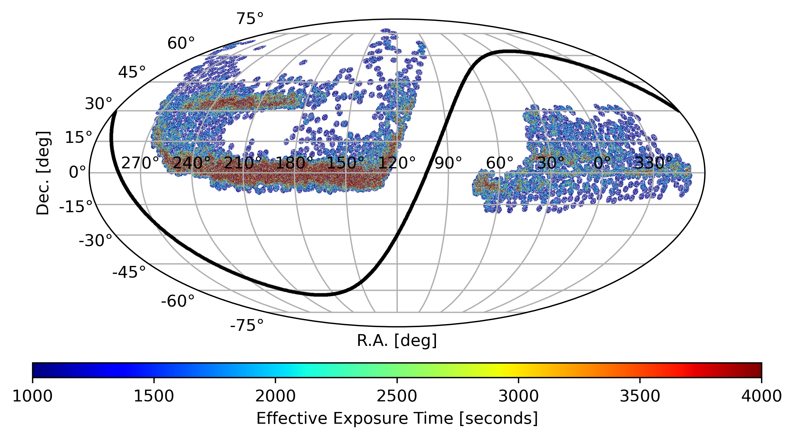
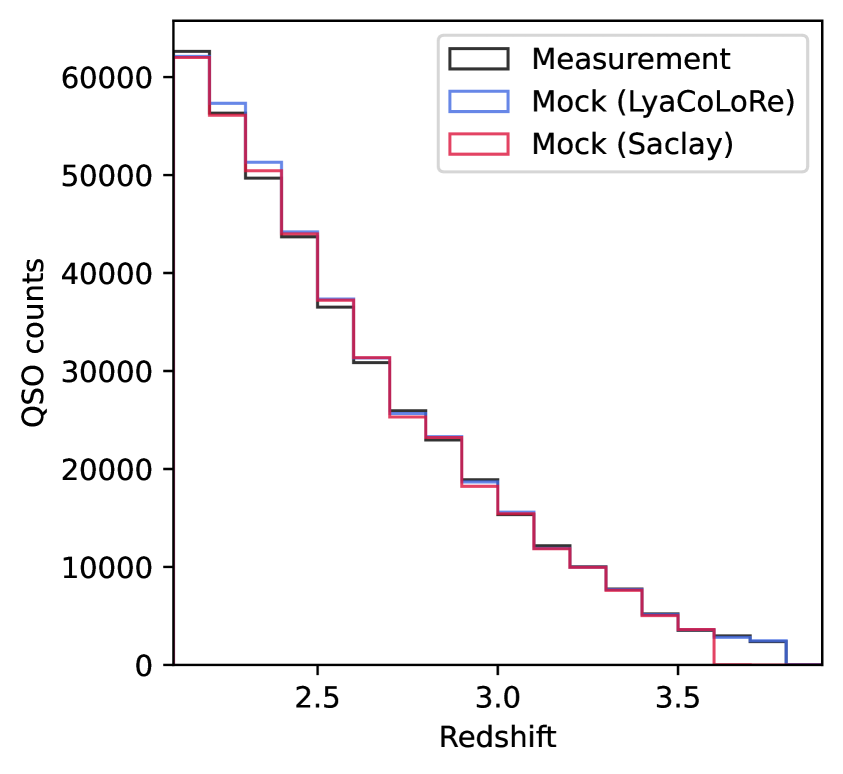
Figure 1: Left: Map of the locations of DESI observations for mock quasars in a DESI DR1 realization. The colours show the assigned effective exposure time. Right: Redshift distributions of one Ly$\alpha$CoLoRe mock and one Saclay mock compared to DESI DR1 quasars over the same redshift range.

Using each of the 150 transmitted flux boxes described in Section 2.1, we generated a synthetic quasar spectra dataset following the same procedure as described in [37], with a modification on the method to mirror the observed footprint and object number density of the DESI DR1. We use the desisim package to simulate both quasar populations and to produce synthetic spectra. The DESI Early Data Release plus two months of observations (EDR+M2) mocks presented in [37] follow a method to emulate the footprint, object number density, and effective exposure time distribution which consists of dividing the observed footprint into HEALpix pixels [42] of nside=16 and then downsampling the available mock quasars to match the density of observed data by HEALpix pixel. This method alters the shape of the quasar auto-correlation function because the exact number of quasars in each HEALpix pixel is related to the strength of the quasar clustering. Therefore, a downsampling factor computed from the ratio between the number of quasars from the simulated box and DESI DR1 over small patches will bias the resulting quasar auto-correlation. To address this issue, we have developed a new methodology that mirrors the spatial inhomogeneities introduced by the DESI survey strategy and does not alter the shape of any of the correlations.

The procedure is as follows. First, we randomly downsample the available targets in the input boxes so that the result follows the expected redshift distribution of the DESI survey and assign a random r-band magnitude to each target following the same procedure as described in Section 3 of [37]. Then, we subdivide the sky into HEALpix pixels of nside=1048. For each pixel, we count the number of tiles on the DESI DR1 footprint that overlap in that region, we refer to this number as the number of passes ($N_{\text{passes}}$). In the observation strategy of the main DESI survey, the maximum number of tiles that can overlap in a given region is seven. The nominal effective exposure time for one DESI observation is 1000 seconds. However, through the DESI survey, Lyman-$\alpha$ quasars will be observed four times for a total effective exposure time of 4000 seconds [43]. Once the number of passes as a function of position in the sky has been computed, we count the total number of observed ($N_{\text{data}}$) and mock ($N_{\text{mock}}$) quasars whose positions are in regions observed by $N_{\text{passes}}=1,2,...,7$ tiles. Finally, we randomly select the mock targets, whose spectra will be simulated, following the ratio $N_{\text{data}}/N_{\text{mock}}$ for each of the possible number of passes. At the same time, we compute a total exposure time probability distribution as a function of $N_{\text{passes}}$, based on the effective exposure time of the observed data quasars defined by $T_{\rm{eff}}=12.15\ \rm{seconds}\times\text{TSNR}^{2}_{\rm{LRG}}$, where $\text{TSNR}_{\rm{LRG}}$ is the signal-to-noise ratio of the LRG template [44]. We use this probability distribution function to randomly assign an integer multiple of 1000 seconds effective exposure time to our mock quasars based on the number of passes corresponding to their position. The result is a preprocessed catalogue of the quasar targets we wish to simulate with exposure times and r-band magnitudes. Finally, we simulate non-linear peculiar velocities (the Fingers of God effect) by adding random Gaussian velocities to our quasars, with a standard deviation of $150$ $\text{km}/\text{s}$. This only affects the Ly$\alpha$-QSO cross-correlation and is subdominant relative to the similar and larger impact of redshift errors [45]. The addition of redshift errors is discussed in Section 2.3 below.

The left panel of Figure 1 shows the resulting footprint and exposure times when applying this procedure to a Ly$\alpha$CoLoRe mock catalogue. The zones with a higher number of passes correspond to those with higher exposure times. Note that before applying the methodology to select the mock quasars, we restrict the redshift range of the observed data catalogue to match the range in the input boxes, $z<3.8$ for Ly$\alpha$CoLoRe, and $z<3.6$ for Saclay. The comparison of the observed redshift distribution with the results from one realization of each type of mock is shown in the right panel of the same figure.

2.3 Simulating quasar spectra

Once we have a catalogue of quasars with associated Ly$\alpha$ transmitted flux skewers, we want to turn these skewers into realistic DESI spectra. We use the quickquasars script from the desisim package to generate our synthetic spectra. This script starts by taking the input transmitted flux boxes described in section 2.1, and post-processing them to introduce absorption features due to astrophysical sources (contaminants). Following [37], these include:

• Damped Ly$\alpha$ absorbers (DLAs) that are correlated with the density field (Section 2.1).

• Broad Absorption Lines (BALs) that are randomly added to $16\%$ of the targets [46].

• Higher Lyman lines (up to Ly$\epsilon$) using rescaled versions of the Ly$\alpha$ optical depth skewers based on the oscillator strengths of each transition.

• Metal absorbers using rescaled versions of the Ly$\alpha$ optical depth skewers, with relative absorption strength coefficients ($C_{m}$) tuned through the process described in Section 2.4. We model four metal absorption lines: SiII$(1190)$, SiII$(1193)$, SiIII$(1207)$, and SiII$(1260)$.

Section 2.3 of [37] gives a detailed description of how astrophysical contaminants are included.

Noiseless spectra are generated by multiplying the post-processed transmitted flux (now including contaminants) with templates for the quasars’ unabsorbed spectrum, referred to as the continuum. We use the SIMQSO method in quickquasars to generate the continuum templates. At last, we use the specsim package [47] to introduce instrumental noise to the spectra by emulating the specifications of the DESI spectrograph and nominal observational conditions set by the dark-time program of the main DESI survey. See Section 3.2.4 of [37] for further details. Figure 2 shows an example spectrum of a mock quasar at redshift $z=3.12$ produced with the aforementioned methodology.

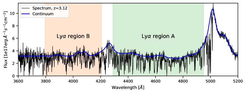
Figure 2: Example synthetic spectrum of a redshift $z=3.12$ quasar as obtained from quickquasars. The blue solid line shows the continuum template used to generate the spectrum prior to introducing instrumental noise. Coloured bands show the Ly$\alpha$ regions A and B.

We also generate in post-processing a contaminated quasar catalogue with random redshift errors following a Gaussian distribution with dispersion $\sigma_{z}=400\ \text{km/s}$. These have a different impact to the non-linear peculiar velocities added in Section 2.2 because they are added after the quasar continua are generated. This leads to the positions of emission lines being randomly shifted relative to the redshift used to generate the quasar continua. For our baseline mocks, we only use the redshift errors in the computation of the Ly$\alpha$-QSO cross-correlation, where they have a smoothing effect similar to non-linear peculiar velocities. However, following [45], we also study their impact on the quasar continuum fitting process in Section 4.4, where the random shifts in the position of the emission lines in the Ly$\alpha$ forest region can introduce spurious correlations.

2.4 Metal tuning

To simulate the contamination by metal lines, we start with the Ly$\alpha$ optical depth skewers and re-scale the optical depth by a scaling factor ($C_{m}$). These re-scaled skewers are then turned into transmitted flux skewers and shifted in wavelength such that they simulate absorption by the corresponding metal line. See [37] for a detailed description of this process. One important factor to note is that the RSD effect is already present in the optical depth skewers used for this, which means metals in the mocks have an RSD signal similar to Ly$\alpha$, with RSD parameter $\beta\sim 1.5$ [37]. This is in contrast to real data, where metals are associated with galaxies, and therefore have a smaller RSD parameter, $\beta\sim 0.5$. We will discuss the impact of this approximation later on in Section 3.4.

For previous mock data sets, the re-scaling factor has been tuned such that the observed metal contamination in the resulting Ly$\alpha$ correlation functions matches the metal contamination measured from eBOSS data [31, 37]. The DESI DR1 Ly$\alpha$ forest data set has significantly more quasar spectra than eBOSS, which means the measurements presented in DESI2024-Ly$\alpha$ are now the most precise Ly$\alpha$ forest correlation function measurements. Therefore, we have used the DESI DR1 measurements to re-tune the values of $C_{m}$.

In order to match the simulated metal contamination in our mocks to the contamination observed in the data, we performed an iterative process that involves the following steps. First, we assume some values for the relative strength coefficients of the four metal lines we wish to simulate, and then create a set of 5 DESI DR1 mock data sets using the metal contamination set by those values. After that, we measured the Ly$\alpha$ correlation functions (all four correlations presented in Section 3.2), and jointly fit these correlations using the model described in Section 3.4 to measure the linear bias parameters for the four metal lines. [37] found a linear relation between the measured bias parameters and the relative strengths $C_{m}$, which means we can use the ratio between the biases measured in mocks versus data to compute the next $C_{m}$ estimates. We found that we only need to perform this process once or twice to be able to reproduce the measured metal biases from DESI2024-Ly$\alpha$ (i.e. it quickly converges).

		Relative strength ($C_{m}\times 10^{3}$)
Metal line	$\lambda_{m}$ [Å]	Ly$\alpha$CoLoRe	Saclay	$\Delta r_{||}$ [ $h^{-1}\text{Mpc}$]
SiIII	1207	3.5	1.6	-21
SiII	1190	1.4	0.68	-53
SiII	1193	0.7	0.53	-60
SiII	1260	1.3	0.57	103

Table 1: The four metal lines we use to simulate metal absorption contaminating the Ly$\alpha$ forest region. The contamination from these metal lines is based on a re-scaling of Ly$\alpha$ optical depth skewers. We show the relative strength coefficients ($C_{m}$) used to perform this re-scaling for both Ly$\alpha$CoLoRe and Saclay mocks. We also show the effective separation in comoving coordinates between each metal line and the Ly$\alpha$ line.

We show the resulting values for the relative strength coefficients $C_{m}$ of the four silicon lines we simulate in Table 1. The tuning process was performed independently for Ly$\alpha$CoLoRe and Saclay mocks, because we do not expect the metal contamination to be the same in both types of mocks. Indeed, the values of $C_{m}$ we obtain for the two types of mocks are fairly different. This can be explained by the fact that the fit of the metal biases is driven by the very small-scale line-of-sight cross-correlation between metal absorption and either Ly$\alpha$ or quasars (i.e. the metal peaks present in Ly$\alpha$ correlation functions). As described in Section 2.1, the main differences between Saclay and Ly$\alpha$CoLoRe mocks are due to the strength of the small-scale quasar clustering (which affects metal peaks in the Ly$\alpha$-QSO cross-correlation) and the RSD signal (which affects line-of-sight correlations). Table 1 also contains the effective difference in co-moving coordinates between the Ly$\alpha$ line and each metal transition. This difference is given by the separation along the line-of-sight at which we see the Ly$\alpha$-Metal cross-correlation peak in our measured correlation functions (see Section 3.4). Note that these values are slightly different for DESI compared to BOSS and eBOSS because they rely on the redshift distribution of our pixel pairs [31, 1].

3 Analysis

As the main goal of this work is to validate the DESI Ly$\alpha$ forest BAO measurement, our analysis process follows closely the analysis done on DESI DR1 data (DESI2024-Ly$\alpha$). The first two parts of the analysis, involve computing the Ly$\alpha$ flux overdensity ($\delta$) field (Section 3.1) and the 3D correlation functions (Section 3.2). To compute these, we use the publicly available picca package. The algorithm behind picca has been described in detail in [31] and [48]. Therefore, we only give a brief overview here, focusing on the parts that are most relevant to our analysis.

One of the main improvements in the DESI DR1 analysis is that we now take into account the cross-covariance between the different correlation functions. This means we need to compute a covariance matrix that covers all four correlation functions. We describe the process for computing this larger covariance matrix in Section 3.3.

The final step of our analysis involves building a model for the correlation functions we have computed, and fitting for the BAO signal. This is achieved using the publicly available Vega package. We give a detailed description of this model in Section 3.4. While the analysis process up to this point is the same as the one used for the real DESI data, our model is slightly different than the one used in DESI2024-Ly$\alpha$. These small differences are described in detail below, and we also discuss their impact on BAO measurements in Section 5.

3.1 The Ly$\alpha$ flux overdensity field

Before measuring the flux overdensity field, we first mask BALs and DLAs present in the spectra. We use the true BAL and DLA catalogues because running the BAL and DLA finders on the entire set of mocks is not computationally feasible. However, we have tested running them on one individual mock and we found it has negligible impact on the BAO measurement from that mock. For studies on the performance of the DLA finder in the context of DESI mocks see [49], and for a detailed description of the BAL and DLA masking process see [48]. Following [50], we keep all BAL quasars and mask their absorption features. For DLAs, we follow [48] and mask all DLAs with column densities $\log N_{\mathrm{H}\textsc{i}}>20.3$. The mask is applied to the region where the DLA leads to more than $20\%$ absorption, while the rest of the DLA wings are corrected using a Voigt profile [51].

The flux overdensity field in the spectrum of a quasar $q$ at observed wavelength $\lambda$ is given by:

$$\delta_{q}(\lambda)=\frac{f_{q}(\lambda)}{\overline{F}(\lambda)C_{q}(\lambda)}-1,$$ (3.1)

where $f_{q}$ is the measured flux, $\overline{F}$ is the global mean Ly$\alpha$ flux, and $C_{q}$ is the quasar continuum. In general, we do not know the true quasar continuum, so we fit it along with $\overline{F}$ directly from the data [31, 48]. This involves expressing the product $\overline{F}(\lambda)C_{q}(\lambda)$ as:

$$\overline{F}(\lambda)C_{q}(\lambda)=\overline{C}(\lambda_{\rm RF})\left(a_{q}+b_{q}\frac{\Lambda-\Lambda_{min}}{\Lambda_{max}-\Lambda_{min}}\right),$$ (3.2)

where $\overline{C}(\lambda_{\rm RF})$ is a universal function of rest-frame wavelength ($\lambda_{\rm RF}$) and $\Lambda\equiv\log\lambda$. The parameters $a_{q}$ and $b_{q}$ are the amplitude and slope that we fit individually for each quasar spectrum in order to account for quasar spectral diversity. This fit also requires an estimate of the total flux variance $\sigma^{2}_{q}(\lambda)$. Following [48], this is given by:

$$\sigma_{q}^{2}(\lambda)=\eta_{\rm pip}(\lambda)\sigma_{\rm pip,q}^{2}(\lambda)+\sigma_{\rm LSS}^{2}(\lambda)[\overline{F}(\lambda)C_{q}(\lambda)]^{2},$$ (3.3)

where $\sigma_{\rm pip,q}$ is usually the flux variance estimated by the DESI pipeline, but in our case it is the variance of the simulated noise in our synthetic spectra. $\eta_{\rm pip}(\lambda)$ is a correction factor meant to account for inaccuracies in the variance estimate, and $\sigma_{\rm LSS}(\lambda)$ is the intrinsic large-scale structure (LSS) variance.

The process of continuum fitting involves an iteration that starts with an estimate of the global quantities $\overline{C}(\lambda_{\rm RF})$, $\eta_{\rm pip}(\lambda)$, and $\sigma_{\rm LSS}(\lambda)$. We then fit the $a_{q}$ and $b_{q}$ parameters for each spectrum and measure the $\delta_{q}(\lambda)$. After that, we measure the variance of this field and fit for the $\eta_{\rm pip}(\lambda)$ and $\sigma_{\rm LSS}(\lambda)$ functions. Finally, we measure the global mean continuum $\overline{C}(\lambda_{\rm RF})$, and then repeat this iterative process until convergence. In practice, 5 steps are enough to achieve convergence [31]. For a detailed description of this process see [48].

We measure the Ly$\alpha$ flux overdensity field in two distinct regions, which we refer to as regions A and B. Region A is located between the Ly$\alpha$ and Ly$\beta$ peaks in the rest-frame wavelength interval $1040-1205$ Å. Region B is located between the Ly$\beta$ peak and the Lyman limit, in the interval $920-1020$ Å. Note that even though region B also contains Ly$\beta$ and higher order absorption lines, we only work with the Ly$\alpha$ flux here. Therefore, we will use the symbol Ly$\alpha$(A) for Ly$\alpha$ region A, and Ly$\alpha$(B) for Ly$\alpha$ region B. The continuum fitting process is performed separately for the two regions. For a comparison of the performance of this continuum fitting method in our mocks versus the real data, see Section 4.2 of [37].

The continuum fitting process also has an unintended effect that has a large impact on the measured correlation functions. This arises due to the amplitude and slope parameters that we fit to each quasar spectrum. While the purpose of these parameters is to account for quasar spectral diversity, they also capture some large-scale structure information. In particular, this model will also fit any large-scale mode of the size of the forest and larger that is present in the data. This biases the measured $\delta$ towards zero, and results in a distortion of the measured correlation functions. Following [27], we account for this distortion by building projection matrices $\eta_{ij}$, such that:

$$\sum_{j}\eta_{ij}\delta^{m}(\lambda_{j})=\sum_{j}\eta_{ij}\delta^{t}(\lambda_{j}),$$ (3.4)

where $\delta^{m}$ is the measured flux overdensity after continuum fitting, $\delta^{t}$ is the true flux overdensity. The equality in Equation 3.4 is not exact on a per-forest basis due to noise, but the formalism is built on the assumption that the two sides converge to equality when averaging over a large enough sample of forests (as we do when we compute correlation functions). The projection matrices are given by:

$$\eta_{ij}=\delta_{ij}^{K}-\frac{w_{j}}{\sum_{k}w_{k}}-\frac{w_{j}\kappa_{i}\kappa_{j}}{\sum_{k}w_{k}\kappa_{k}^{2}},$$ (3.5)

where $\delta_{ij}^{K}$ is the Kronecker delta, $\kappa_{k}=\log\lambda_{k}-\overline{\log\lambda_{q}}$, and the weights $w_{i}$ are described below. For a detailed description of the projection and the assumptions behind it see [27] and [52]. Using this formalism, we project the measured flux overdensity field using the left-hand side of Equation 3.4. However, we model correlation functions (not the $\delta$ field), so the right-hand side is instead propagated into our correlation function model. We describe this process in Section 3.4.

The weights used to build projection matrices are the same weights we use to compute correlation functions, and are given by:

$$w(\lambda_{i})=\frac{[(1+z_{i})/(1+2.25)]^{\gamma_{{\rm Ly}\alpha}-1}}{\eta_{\rm LSS}\sigma_{\rm LSS}^{2}(\lambda)+\eta_{pip}(\lambda)\tilde{\sigma}_{pip,q}^{2}(\lambda)},$$ (3.6)

where $\tilde{\sigma}_{pip,q}^{2}=\sigma_{pip,q}^{2}/[\overline{F}(\lambda)C_{q}(\lambda)]^{2}$, and we take into account the redshift evolution of the Ly$\alpha$ bias using $\gamma_{{\rm Ly}\alpha}=2.9$ based on [53]. The $\eta_{\rm LSS}$ term is an ad-hoc correction factor that modulates the relative importance of instrumental noise versus intrinsic Ly$\alpha$ fluctuations. This was introduced following the study by [48] to minimize the uncertainties in the correlation function estimates. For our dataset, [48] found $\eta_{\rm LSS}=7.5$ to be the optimal value.

3.2 Estimating correlation functions

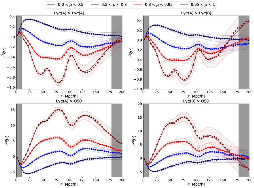
Figure 3: Stacked correlation functions from a set of 100 DESI DR1 Ly$\alpha$CoLoRe mocks compressed into $\mu=r_{||}/r$ wedges and shown as a function of isotropic separation $r$ (points with error-bars). The four panels each show one of the four correlation functions we compute, with the two auto-correlations on the top row, and the two cross-correlations on the bottom row. The shaded regions indicate the DESI DR1 uncertainties, and the lines indicate the best-fit model described in Section 3.4.

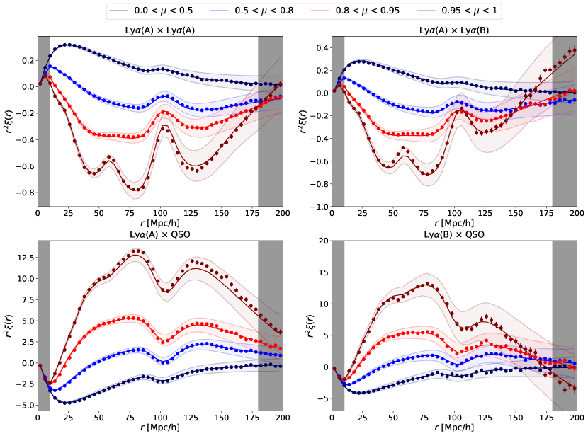
Figure 4: Similar to Figure 3, but showing the stack of correlation functions measured from 50 DESI DR1 Saclay mocks.

For the DESI high redshift BAO measurement, we use both the Ly$\alpha$ forest and quasars as tracers of large-scale structure. As discussed above, we measure the Ly$\alpha$ flux overdensity field in two separate regions of our spectra. Therefore, we have six different two-point functions that can be computed from these three datasets (Ly$\alpha$(A), Ly$\alpha$(B), and QSOs). Following [31], we focus on a subset of four correlations. These include two auto-correlations of Ly$\alpha$ flux, Ly$\alpha$(A)$\times$Ly$\alpha$(A) and Ly$\alpha$(A)$\times$Ly$\alpha$(B), and two cross-correlations between Ly$\alpha$ flux and quasars, Ly$\alpha$(A)$\times$QSO and Ly$\alpha$(B)$\times$QSO.

We compute correlation functions on a grid in comoving separation along ($r_{||}$) and across ($r_{\bot}$) the line-of-sight. These are computed from the measured angles $\theta$ and redshifts $z$ using a fiducial cosmology. For two pixels, $i$ and $j$, separated by $\Delta\theta$, the comoving separations are given by [29]:

$$r_{||} =[D_{\mathrm{c}}(z_{i})-D_{\mathrm{c}}(z_{j})]\cos{\frac{\Delta\theta}{2}},$$ (3.7)

$$r_{\bot} =[D_{\mathrm{M}}(z_{i})+D_{\mathrm{M}}(z_{j})]\sin{\frac{\Delta\theta}{2}},$$ (3.8)

where $D_{\mathrm{c}}$ and $D_{\mathrm{M}}$ are the radial and transverse comoving distances. As mentioned in Section 2.1, we use the Planck 2015 results [40] as our fiducial cosmology. Besides $r_{||},r_{\bot}$, we will use the $r,\mu$ parametrization when presenting correlation functions, where $r^{2}=r_{||}^{2}+r_{\bot}^{2}$ and $\mu=r_{||}/r$. We compute correlation functions in bins of $4$  $h^{-1}\text{Mpc}$ in both $r_{||}$ and $r_{\bot}$. For auto-correlations, we use a grid between $0$ and $200$  $h^{-1}\text{Mpc}$ for both coordinates, resulting in a $50\times 50$ grid. On the other hand, for cross-correlations we distinguish between pixels in front of (negative $r_{||}$) and behind quasars (positive $r_{||}$), so $r_{||}$ takes values between $-200$ and $200$  $h^{-1}\text{Mpc}$, resulting in a $100\times 50$ grid.

To measure correlation functions, we follow previous Ly$\alpha$ forest BAO analyses [27, 31, 54] and use a weighted pair-counting algorithm. The Ly$\alpha$ flux auto-correlation and its cross-correlation with quasars are given by:

$$\xi_{M}=\frac{\sum_{i,j\in M}w_{i}w_{j}\delta_{i}\delta_{j}}{\sum_{i,j\in M}w_{i}w_{j}},$$ (3.9)

where $M$ defines a bin in comoving coordinates, and $\delta=1$ for quasars. The sums run over pixel-pixel pairs for the auto-correlation and over pixel-QSO pairs for the cross-correlation. The weights for the Ly$\alpha$ forest are given by Equation 3.6, while for quasars they are given by:

$$w_{Q}=[(1+z_{Q})/(1+2.25)]^{\gamma_{Q}-1},$$ (3.10)

where $\gamma_{Q}=1.44$ based on measurements by [55].

For our validation study, we also compute the mean and covariance of correlation functions from sets of many mocks. We refer to these as stacked correlation functions. This gives us measurements of the correlation function with negligible statistical uncertainties. Therefore, they can be used to test our model and BAO measurement with much greater statistical precision than an individual mock would allow (Section 4.1). We show the stacked correlation functions from the set of 100 Ly$\alpha$CoLoRe mocks in Figure 3, and from the 50 Saclay mocks in Figure 4. For a comparison of correlations functions measured from Ly$\alpha$CoLoRe and Saclay mocks, as well as DESI data, see [37].

3.3 Covariance matrix

The biggest change between the DESI 2024 Ly$\alpha$ BAO analysis and previous analyses on DESI EDR and SDSS data is how we compute the covariance matrix. The change is that we now compute one covariance matrix for all four correlation functions, which means we also take into account the cross-covariances between the individual correlations. In previous datasets these were found to be negligible [e.g. 31]. However, that is not the case for DESI DR1, where ignoring these cross-covariances leads to a $\sim 10\%$ change in BAO uncertainties. The analysis that led to this decision is described in DESI2024-Ly$\alpha$.

To compute the $15000\times 15000$ covariance matrix we follow the same approach used in previous analyses [e.g. 27, 28, 31]. We first compute correlation functions independently in each HEALPix pixel. For the DESI DR1 dataset, there are $1028$ pixels (nside $=16$), each covering a roughly $250\times 250\;(h^{-1}\mathrm{Mpc})^{2}$ patch at $z_{\mathrm{eff}}=2.33$. We then compute a noisy estimate of the covariance matrix from this sample of correlation function measurements:

$$C_{MN}=\frac{1}{W_{M}W_{N}}\sum_{s}W_{M}^{s}W_{N}^{s}[\xi_{M}^{s}\xi_{N}^{s}-\xi_{M}\xi_{N}],$$ (3.11)

where $s$ is a sub-sample, $W_{M}^{s}=\sum_{i\in M,s}w_{i}$, and $W_{M}=\sum_{s}W_{M}^{s}$. Finally, the noisy estimate of the covariance is smoothed at the level of the correlation matrix given by:

$$\text{Corr}_{MN}\equiv C_{MN}/(C_{MM}C_{NN})^{1/2},$$ (3.12)

where $C_{MM}$ and $C_{NN}$ are the variances in bins $M$ and $N$ respectively. The smoothing is done by replacing non-diagonal elements of the correlation matrix which correspond to the same differences $|r_{||}(M)-r_{||}(N)|$ and $|r_{\bot}(M)-r_{\bot}(N)|$ with their average. This method has proven effective for obtaining estimates of the covariance matrices of individual correlations in the past [see 26, 31]. However, for DESI DR1 we employ it to obtain an estimate of the much larger covariance matrix of all four correlations.

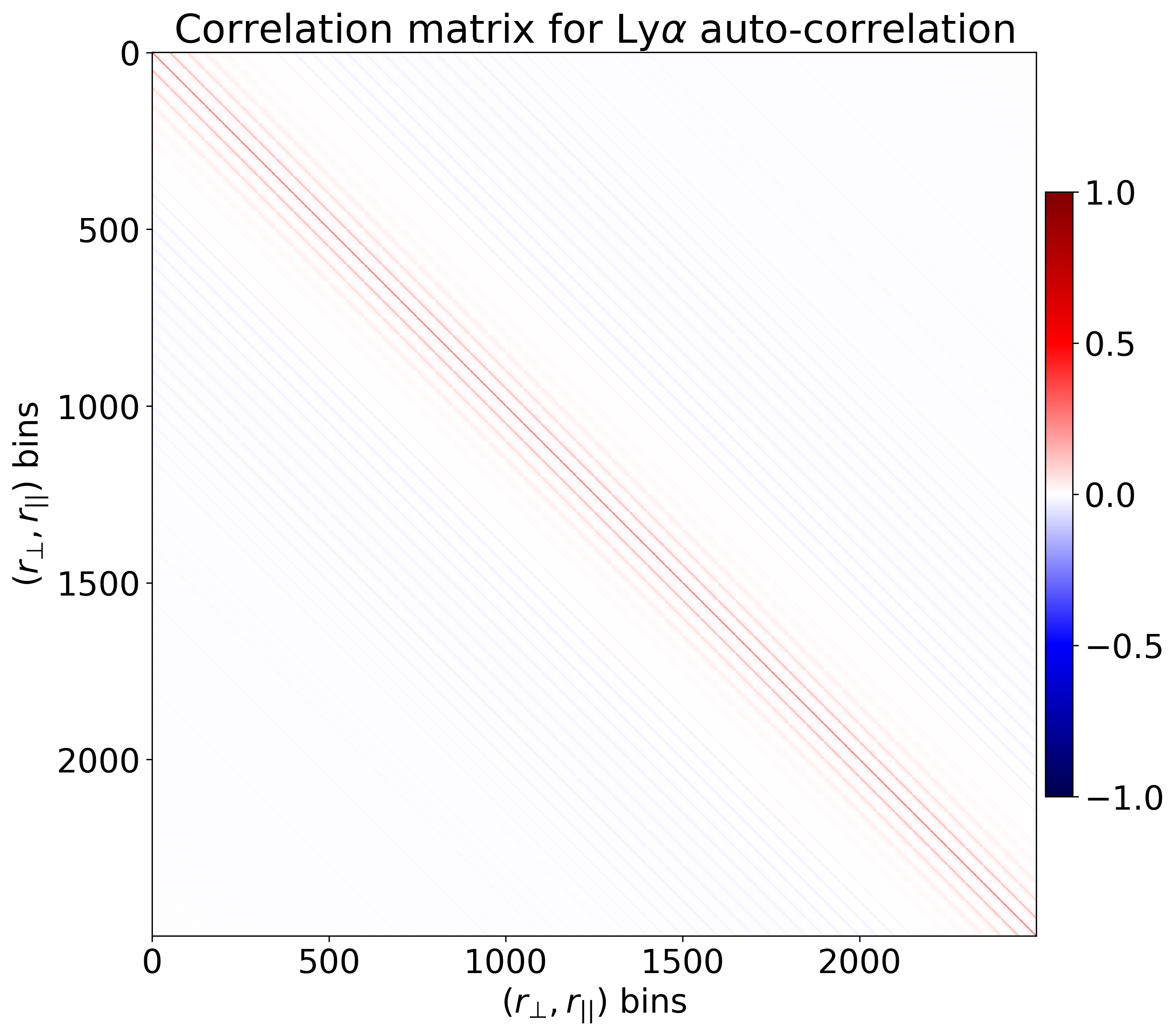
Figure 5: Normalized smoothed covariance matrix (correlation matrix) for the Ly$\alpha$ auto-correlation function computed from the stack of 100 Ly$\alpha$CoLoRe mocks. This is part of the larger correlation matrix of all four Ly$\alpha$ correlations. The off-diagonal lines visible in this figure are the correlations between line-of-sight bins for the same $r_{\bot}$. The most important correlations are between neighbouring $r_{||}$ bins (i.e. $\Delta r_{||}=4$ $h^{-1}\text{Mpc}$) which are $\sim 0.3$ in magnitude (first off-diagonal lines visible here), with correlations at larger $\Delta r_{||}$ rapidly decaying to below $|0.1|$.

Using this procedure we compute an individual smoothed covariance matrix for each of the 150 mocks. We use separate covariance matrices for each mock in order to mimic the analysis of the DESI DR1 data (DESI2024-Ly$\alpha$). For the stacked correlation functions, we first gather the correlation function samples from each mock and then compute the covariance matrix using the same method. This means we use much larger sets of samples for the covariance matrices of the stacked correlations ($\sim 100$k for Ly$\alpha$CoLoRe, and $\sim 50$k for Saclay). We will use these stacked covariance matrices to test our method for estimating the full covariance of individual mocks in Section 4.3.

The covariance matrices for 2 out of the 150 mocks are not positive semi-definite even after smoothing. In order to use them for our analysis, we combine the correlation matrix from the stack of mocks with the variance estimates of each of the two mocks. Note that this only affects our studies of the population of mock results, and not the results from the stacked correlation functions. Furthermore, we have also performed the entire analysis with the two mocks discarded, and it did not significantly impact any of our results or conclusions.

The smoothed correlation matrix of the Ly$\alpha$ auto-correlation function from the stack of 100 Ly$\alpha$CoLoRe mocks is shown in Figure 5. For visualization purposes, we only show a subset of the larger correlation matrix. We also show the cross-correlation matrix between Ly$\alpha$(A)$\times$Ly$\alpha$(A) and Ly$\alpha$(A)$\times$QSO in Figure 6. The features that dominate the covariance matrix are the off-diagonal lines at regular intervals of 50 bins. These represent the correlations between line-of-sight bins at the same transverse separation (i.e. $\Delta r_{||}>0$ $h^{-1}\text{Mpc}$, $\Delta r_{\bot}=0$ $h^{-1}\text{Mpc}$). The most important of these are correlations between neighbouring line-of-sight bins ($\Delta r_{||}=4$ $h^{-1}\text{Mpc}$), which are $\sim 0.3$ in magnitude (for the auto-covariance). Correlations at larger separations ($\Delta r_{||}>4$ $h^{-1}\text{Mpc}$) rapidly decay below $|0.1|$. We discuss and provide other illustrations of our correlation matrix in Section 4.3.

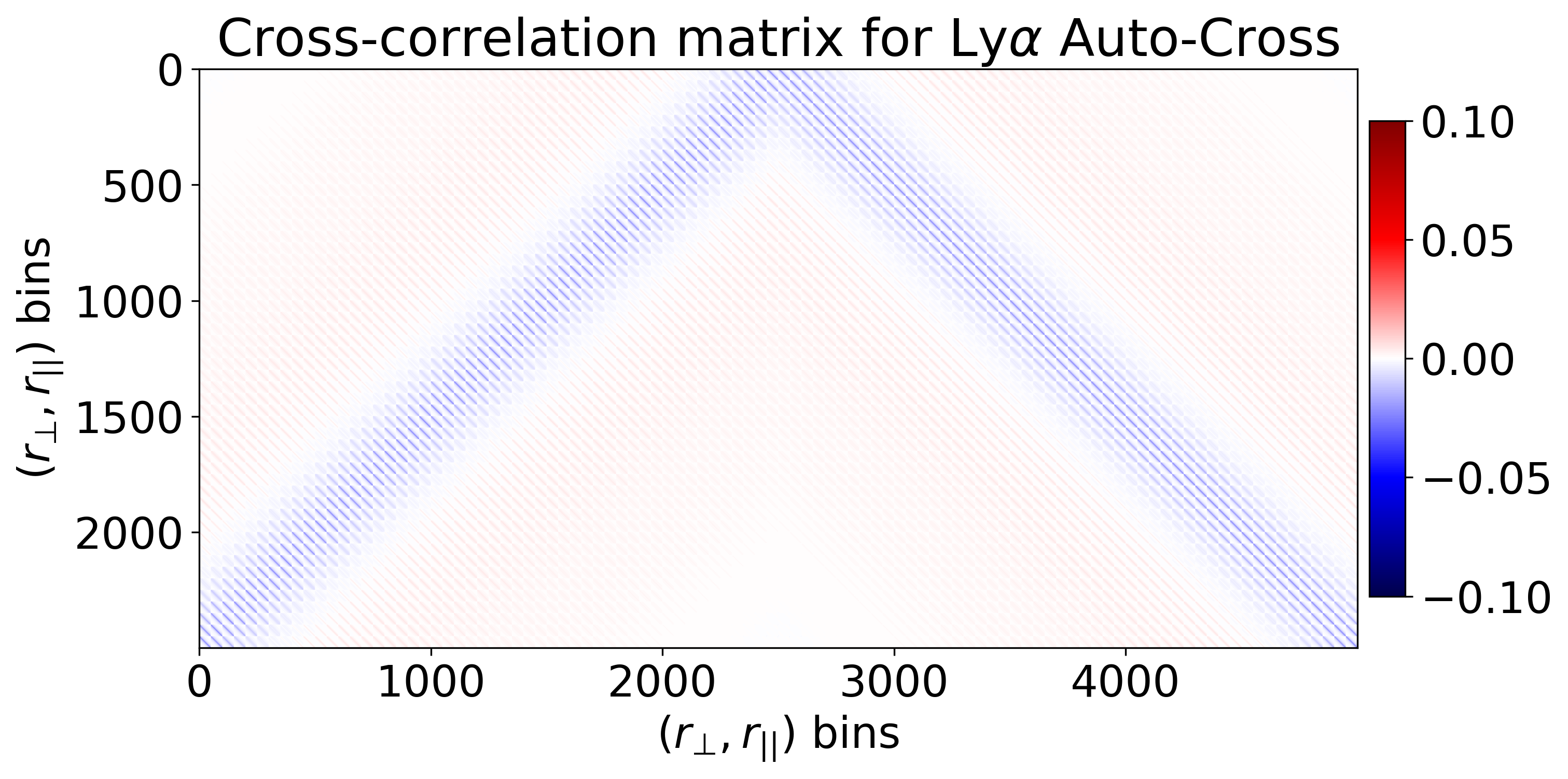
Figure 6: Smoothed cross-correlation matrix between the Ly$\alpha$ auto-correlation and the Ly$\alpha$-QSO cross-correlation from the stack of 100 Ly$\alpha$CoLoRe mocks. Note that the range of the colour scale is 10 times smaller than Figure 5. Unlike previous Ly$\alpha$ BAO analyses, with DESI DR1 this cross-correlation needs to be taken into account, as it leads to $\sim 10\%$ changes in the BAO uncertainties. The structure can be understood when considering that the Ly$\alpha$-QSO cross-correlation is computed on a grid from $-200$ $h^{-1}\text{Mpc}$ to $200$ $h^{-1}\text{Mpc}$, while the Ly$\alpha$ auto-correlation is symmetric along the line-of-sight, and therefore computed on a grid from $0$ $h^{-1}\text{Mpc}$ to $200$ $h^{-1}\text{Mpc}$. The most important correlations are again between neighbouring bins along the line-of-sight (i.e. $\Delta r_{||}=4$ $h^{-1}\text{Mpc}$, $\Delta r_{\bot}=0$ $h^{-1}\text{Mpc}$).

3.4 Modelling correlation functions

Our model for the Ly$\alpha$ forest correlation functions is based on a template approach that was first introduced in [22]. We start with an isotropic linear matter power spectrum $P_{\mathrm{fid}}$, that is split into a peak (or wiggles) component $P_{\mathrm{fid}}^{\mathrm{p}}$, and a smooth (or no-wiggles) component $P_{\mathrm{fid}}^{\mathrm{s}}$. This represents our template. The modelling process involves adding the Kaiser term [56], as well as models for non-linearities, some contaminants, and various other effects we need to account for. The now anisotropic power spectrum model is then transformed into a correlation function model and interpolated on a grid in $r_{||}$ and $r_{\bot}$. Finally, we add the effect of metal contamination and distortion due to continuum fitting. The entire process is performed separately for the smooth and peak components of the template, and the final step involves combining them. The BAO feature is measured by allowing the coordinates ($r_{||},r_{\bot}$) of the peak component to vary using two scale parameters ($\alpha_{||}$,$\alpha_{\bot}$) which are described below. We use the Vega package to model and fit our correlation functions.

The isotropic linear matter power spectrum $P_{\mathrm{fid}}$ is computed using CAMB [57] and the same fiducial cosmology above [40]. The decomposition into peak and smooth components is performed using the algorithm described in [22]. The anisotropic model cross-spectrum is given by:

$$P_{A\times B}(k,\mu_{k},z)=b_{A}b_{B}(1+\beta_{A}\mu_{k}^{2})(1+\beta_{B}\mu_{k}^{2})\;G(k,\mu_{k})F_{\mathrm{SM}}(k,\mu_{k})F_{\mathrm{NL}}(k,\mu_{k})P_{\mathrm{fid}}(k),$$ (3.13)

where ($A$, $B$) are either (Ly$\alpha$, Ly$\alpha$) for auto-correlations, or (Ly$\alpha$, QSO) for cross-correlations. $b_{X}$ and $\beta_{X}$ are the linear bias and RSD parameters (for $X$ either Ly$\alpha$ or QSO), and $\mu_{k}=k_{||}/k$ with isotropic wavenumber $k$, and line-of-sight wavenumber $k_{||}$. $G(k,\mu_{k})$ models the binning of the correlation function and is given by: $G(k,\mu_{k})=\mathrm{sinc}(k_{||}R_{||}/2)\;\mathrm{sinc}(k_{\bot}R_{\bot}/2)$, with bin sizes $R_{||}=R_{\bot}=4$  $h^{-1}\text{Mpc}$. $F_{\mathrm{SM}}$ and $F_{\mathrm{NL}}$ are the smoothing and redshift error models respectively, and are described below.

The Ly$\alpha$ $\delta$ field also contains absorption from unmasked HCDs that are too small to be detected. As these HCDs also trace the underlying large-scale structure, their auto- and cross-correlations with Ly$\alpha$ and QSOs need to be modelled. Following [58], these can be added to our model by simply treating the bias and RSD parameters associated with the Ly$\alpha$ forest as effective parameters ($b^{\prime}_{\mathrm{Ly}\alpha},\beta^{\prime}_{\mathrm{Ly}\alpha}$) that include both Ly$\alpha$ and HCDs. These are given by:

$$b^{\prime}_{\mathrm{Ly}\alpha} =b_{\mathrm{Ly}\alpha}+b_{\mathrm{HCD}}F_{\mathrm{HCD}}(k_{||}),$$ (3.14)

$$b^{\prime}_{\mathrm{Ly}\alpha}\beta^{\prime}_{\mathrm{Ly}\alpha} =b_{\mathrm{Ly}\alpha}\beta_{\mathrm{Ly}\alpha}+b_{\mathrm{HCD}}\beta_{\mathrm{HCD}}F_{\mathrm{HCD}}(k_{||}),$$ (3.15)

where parameters with subscript Ly$\alpha$ are associated with the IGM, and parameters with subscript HCD are associated with high column-density absorbers. The function $F_{\mathrm{HCD}}(k_{||})$ depends on the column density distribution function of the HCDs present in our data [59, 58]. However, measurements of this function in the $N_{\mathrm{H}\textsc{i}}$ range of interest ($\log N_{\mathrm{H}\textsc{i}}<20.3$) are very limited [60, 61, 51, 62]. Therefore, we use the approximate form $F_{\mathrm{HCD}}=\exp(-L_{\mathrm{HCD}}k_{||})$, where $L_{\mathrm{HCD}}$ can be interpreted as the typical length scale of unmasked HCDs [29]. Following [63], and in line with DESI2024-Ly$\alpha$, we treat $L_{\mathrm{HCD}}$ as a free parameter that we marginalize over. For a comparison of the different HCD models, see Appendix A of DESI2024-Ly$\alpha$.

In our mocks, the $F_{\mathrm{NL}}(k,\mu_{k})$ term only applies to the Ly$\alpha$-QSO cross-correlation and models the statistical quasar redshift errors and quasar non-linear velocities. For the analysis on data, DESI2024-Ly$\alpha$ test both a Lorentzian and a Gaussian smoothing, following [64]. These are given by:

$$F^{2}_{\mathrm{NL,Lorentz}} =[1+(k_{||}\sigma_{z})^{2}]^{-1},$$ (3.16)

$$F^{2}_{\mathrm{NL,Gauss}} =\exp\bigg{[}-\frac{1}{2}(k_{||}\sigma_{z})^{2}\bigg{]},$$ (3.17)

where $\sigma_{z}$ is a free parameter. As our redshift errors were injected using a Gaussian distribution, we use that form for the $F_{\mathrm{NL}}(k,\mu_{k})$ term. However, we also tested the Lorentzian distribution and found that the choice between these two functional forms does not have an impact on BAO measurements. Note that for the analysis on data, DESI2024-Ly$\alpha$ also used a non-linear term for the small scales in the auto-correlation based on [65]. However, we do not use it because our mocks are based on a Gaussian field and therefore do not have the same small-scale non-linearities present in the real data. We have tested adding this model and we found it has no impact on BAO measurements.

The input log-normal simulations have a grid cell size of $\sim 2.4$  $h^{-1}\text{Mpc}$, which results in extra smoothing of the measured correlations functions. Following [35], we add Gaussian anisotropic smoothing to account for this effect, represented by the $F_{\mathrm{SM}}$ term in Equation 3.13. This model has two smoothing scale parameters $(\sigma_{||},\sigma_{\bot})$, which we fit and marginalize over. This is the only component of our model that is present in the analysis on mocks, and absent from the analysis on data.

The next step in the modelling process involves transforming the anisotropic model power spectrum into a model correlation function. This is done by first performing a multipole decomposition up to $\ell=6$, followed by a Hankel transform, and finally computing the two-dimensional correlation function from the correlation multipoles. We have also tested including multiples with $\ell>6$, and found no impact on BAO measurements. We interpolate the model onto a grid with $2$ $h^{-1}\text{Mpc}$ bins in $r_{||}$ and $r_{\bot}$. This is an improvement over previous analyses which used $4$ $h^{-1}\text{Mpc}$ bins and allows us to build a more precise model for the correlation functions.

Besides Ly$\alpha$ flux, we also model the contamination due to metal absorption. This involves computing correlation function models for all Ly$\alpha$-Metal and Metal-Metal cross-correlations using the same framework as for the main Ly$\alpha$ correlations. Each metal line has a separate linear bias and RSD parameters $(b,\beta)$, but we neglect HCD effects for the Ly$\alpha$ part of these correlations. Following previous analyses, we fix the metal RSD parameters to 0.5 [27, 28, 31]. However, given that the metals in our mocks are added by re-scaling the Ly$\alpha$ flux field, their RSD parameters are likely closer to the Ly$\alpha$ RSD parameter ($\sim 1.5$). We have tested that this has a negligible impact on our results. When computing correlation functions we assume all pixels are caused by Ly$\alpha$ absorption. As some of the absorption is caused by metal lines, we assign these pixel pairs to the wrong correlation function bins. Following [27, 28], we model this through the use of metal matrices which transform model metal correlations from their correct separations $(\tilde{r}_{||},\tilde{r}_{\bot})$ to the coordinate grid of the measured correlations:

$$\xi_{\mathrm{m}}^{M}=\sum_{N}M_{MN}\xi_{\mathrm{m}}(\tilde{r}_{||}(N),\tilde{r}_{\bot}(N)),$$ (3.18)

with the metal matrix:

$$M_{MN}=\frac{1}{W_{M}}\sum_{(i,j)\in M,(i,j)\in N}w_{i}w_{j},$$ (3.19)

where $(i,j)\in M$ refers to bins computed using the assumed (wrong) redshifts, $(i,j)\in N$ refers to bins computed using the correct redshifts, and we compute correlations $\xi_{m}$ for metal lines $m$ described below. One major change for the DESI DR1 analysis is that we now compute the sum in Equation 3.19 only as a function of $r_{||}$, and ignore the few per cent changes in $r_{\bot}$. Previous analyses computed these matrices numerically using a small fraction of the pairs available ($\sim 0.1\%$), which was not precise enough and very expensive computationally. This simplification allows us to obtain a more precise measurement of the metal contamination when working with the smaller $2$ $h^{-1}\text{Mpc}$ bins.

We model the contamination from the four metal lines in Table 1: SiIII$(1207)$, SiII$(1190)$, SiII$(1193)$, and SiII$(1260)$. The correlation model including metal contamination is given by:

$$\xi^{t}_{\mathrm{Ly}\alpha\times X}=\xi_{\mathrm{Ly}\alpha\times X}+\sum_{m}\xi_{X\times m}+\sum_{m_{1},m_{2}}\xi_{m_{1}\times m_{2}},$$ (3.20)

where the sums are performed over the four metal lines, and $X$ stands for Ly$\alpha$ in the auto-correlation model, and for QSO in the cross-correlation model.

The only missing ingredient in $\xi^{t}$ is the effect of the distortion due to continuum fitting errors. As discussed in Section 3.1, we use a projection formalism to account for this effect. This includes forward modelling the projection matrices computed for each forest (Equation 3.4) into distortion matrices given by:

$$D_{MN}^{\mathrm{auto}} =\frac{1}{W_{M}}\sum_{i,j\in M}w_{i}w_{j}\sum_{i^{\prime},j^{\prime}\in N}\eta_{ii^{\prime}}\eta_{jj^{\prime}},$$ (3.21)

$$D_{MN}^{\mathrm{cross}} =\frac{1}{W_{M}}\sum_{i,j\in M}w_{i}w_{j}\sum_{i^{\prime},j\in N}\eta_{ii^{\prime}},$$ (3.22)

with the first equation giving the distortion matrix for the auto-correlation, and the second giving the distortion matrix for the cross-correlation. The model bins $N$ are $2$ $h^{-1}\text{Mpc}$ in size, while the data bins $M$ are $4$ $h^{-1}\text{Mpc}$ in size. This means the distortion matrices are not square. The distorted correlation function model is given by:

$$\hat{\xi}_{M}=\sum_{N}D_{MN}\xi_{N}^{t}.$$ (3.23)

As mentioned above, the final step of our modelling process involves combining the peak and smooth components, which have so far gone through the modelling process independently. The final model is given by:

$$\xi(r_{||},r_{\bot})=\hat{\xi}_{\mathrm{s}}(r_{||},r_{\bot})+\hat{\xi}_{\mathrm{p}}(\alpha_{||}r_{||},\alpha_{\bot}r_{\bot}),$$ (3.24)

where $\alpha_{||}$ and $\alpha_{\bot}$ are scale parameters that we fit for. These correspond to:

$$\alpha_{||}=\frac{D_{H}(z)/r_{d}}{[D_{H}(z)/r_{d}]_{fid}},\;\;\alpha_{\bot}=\frac{D_{M}(z)/r_{d}}{[D_{M}(z)/r_{d}]_{fid}},$$ (3.25)

where $r_{d}$ is the scale of the sound horizon at the end of the drag epoch, the $fid$ subscript indicates the values computed in the fiducial cosmology, and $D_{H}(z)=c/H(z)$ with Hubble parameter $H(z)$ and speed of light $c$. As discussed in Section 2.1, we use the Planck 2015 results as the fiducial cosmology for all our mocks, which matches the cosmology used to create the Ly$\alpha$CoLoRe mocks but is slightly different than the one used for Saclay mocks (Planck 2018). We account for this small difference by simply rescaling the $\alpha_{||}$ and $\alpha_{\bot}$ results from Saclay mocks by a factor given by the ratios between $[D_{H}(z)/r_{d}]_{fid}$ and $[D_{M}(z)/r_{d}]_{fid}$ in the two cosmologies. This consists of a $\sim 0.02\%$ shift in the BAO position. We also test our sensitivity to the choice of fiducial cosmology in Appendix B.

To obtain posterior distributions for the parameters, we use a Gaussian likelihood and either the minimizer iminuit [67, 68] or the nested sampler PolyChord [69, 70]. iminuit is useful for quickly computing the best-fit model and associated parameter values. However, it approximates parameter uncertainties as Gaussian using the second derivative of the likelihood around the best-fit point. As BAO posteriors can be non-Gaussian [63], the more robust method involves computing the full posterior distribution with PolyChord. However, this is much slower and it is not computationally feasible to run the sampler for all 150 mock analyses. Therefore, we only use the sampler to validate the BAO measurements from the stacked correlations, and on one of the mocks to confirm that the Gaussian approximation works well. We found that for DESI DR1 mock datasets, the BAO posterior distribution is closely Gaussian, and therefore the results from the minimizer can be trusted when studying the population of mocks. We use wide flat priors for all parameters, with the exception of the HCD RSD parameter, $\beta_{\mathrm{HCD}}$, for which we use a Gaussian prior $\mathcal{N}(0.5,0.09^{2})$, in line with previous analyses. The priors are the same as the ones used in DESI2024-Ly$\alpha$.

We show the best-fit model for the stacked Ly$\alpha$CoLoRe correlation functions in Figure 3, and for the Saclay mocks in Figure 4. The figures also include the uncertainties from the DESI DR1 data (shaded regions). The stacked correlations are visually well fit by our model, with the model lines generally going through the data points in most regions. For the few exceptions where the model deviates significantly from the data points (e.g. around the metal peak at $60$ $h^{-1}\text{Mpc}$ in the line-of-sight wedge of auto-correlations), it is still within the shaded region, which indicates that it works well relative to the uncertainties of DESI DR1.

4 Results

We focus on two types of analyses when fitting correlation functions from synthetic data sets. First, we work with stacks of correlation functions in Section 4.1. These allow us to obtain high statistics correlation function measurements, and validate BAO analyses with very high precision. Secondly, we fit each mock individually and study the statistics of the population of resulting BAO measurements in Section 4.2. To further test the robustness of our analysis, we study how sensitive BAO measurements are to different covariance matrix estimates in Section 4.3, and the impact of redshift errors in Section 4.4.

4.1 Fits of stacked correlations

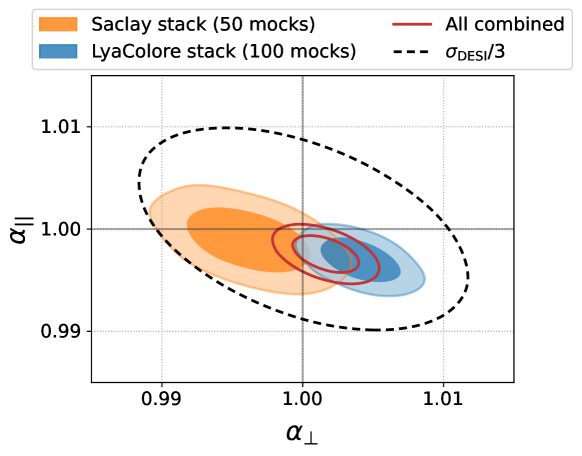
Figure 7: $68\%$ and $95\%$ credible regions of BAO measurements from stacks of 50 Saclay (orange), 100 Ly$\alpha$CoLoRe mocks (blue), and the combination of the two results (red). We measure anisotropic BAO parameterized through the scale parameters $\alpha_{||}$ (along the line-of-sight) and $\alpha_{\bot}$ (across the line-of-sight). The grey cross at $\alpha_{||}=\alpha_{\bot}=1$ indicates the input mock cosmology, while the black dotted contour shows $1/3$ of the DESI DR1 Ly$\alpha$ BAO uncertainty. The $1/3$ bound represents the threshold within which the analysis had to be validated. The mock results are consistent with the truth which indicates any bias in the BAO peak position is negligible relative to our uncertainties.

The main goal of this work is to validate the DESI DR1 Ly$\alpha$ forest BAO measurement using synthetic datasets. To achieve this, we first focus on extracting BAO from stacked correlation functions. We work with the two types of mocks (Ly$\alpha$CoLoRe and Saclay) independently. This means we have two sets of measurements for the four correlation functions: the first from 100 Ly$\alpha$CoLoRe mocks, and the second from 50 Saclay mocks. As we used the same cosmology both to create and to analyse the mocks, we expect to recover $\alpha_{||}=\alpha_{\bot}=1$ in the absence of systematic errors.

The analysis presented here was performed in parallel with the analysis of DESI DR1 data presented in DESI2024-Ly$\alpha$. One of the key requirements for unblinding the data measurement was to recover unbiased BAO measurements from stacks of many mocks that include all of the main Ly$\alpha$ forest contaminants. Concretely, this meant the best-fit measurements from the stacks of mocks needed to be close to the truth to within a certain threshold. This threshold was based on the uncertainty of the DESI DR1 Ly$\alpha$ BAO measurement, and it required the total systematic bias to be smaller than $1/3$ of that uncertainty. For the blinded data this corresponded to $\sim 0.005$ in $\alpha_{||}$ and $\sim 0.007$ in $\alpha_{\bot}$. After unblinding the uncertainties increased slightly, and the new threshold corresponds to $\sim 0.007$ in $\alpha_{||}$ and $\sim 0.008$ in $\alpha_{\bot}$ (DESI2024-Ly$\alpha$). For this manuscript, we show the threshold based on the real unblinded measurement, but note that the tighter requirement based on the blinded data had to be satisfied for the unblinding to take place.

	Ly$\alpha$CoLoRe stack	Saclay stack	Combined
Parameter	(100 mocks)	(50 mocks)	(150 mocks)
$\alpha_{||}$	$0.9970\pm 0.0014$	$0.9992\pm 0.0021$	$0.9976\pm 0.0012$
$\alpha_{\bot}$	$1.0041\pm 0.0018$	$0.9964\pm 0.0029$	$1.0016\pm 0.0015$
$\rho_{\alpha_{||},\alpha_{\bot}}$	-0.49	-0.47	-0.48

Table 2: BAO best fit results (mean of posterior), uncertainties ($68\%$ credible regions), and correlation coefficient $\rho$, measured from stacked correlation functions.

We show the BAO measurements from the two stacks of mocks in Figure 7 (blue and orange contours), and Table 2. Both measurements contain the truth within their $2\sigma$ bound. This indicates there are no systematic effects that significantly bias BAO measurements from our mocks. The red contour shows the combination of the two measurements at the BAO level, which is also unbiased. The threshold mentioned above is shown through the black dashed contour in Figure 7, which marks $1/3$ of the $68\%$ credible region of the data BAO measurement from DESI2024-Ly$\alpha$. Both the best-fit results and the entire $95\%$ credible regions of our measurements are within this bound.

4.2 Population statistics

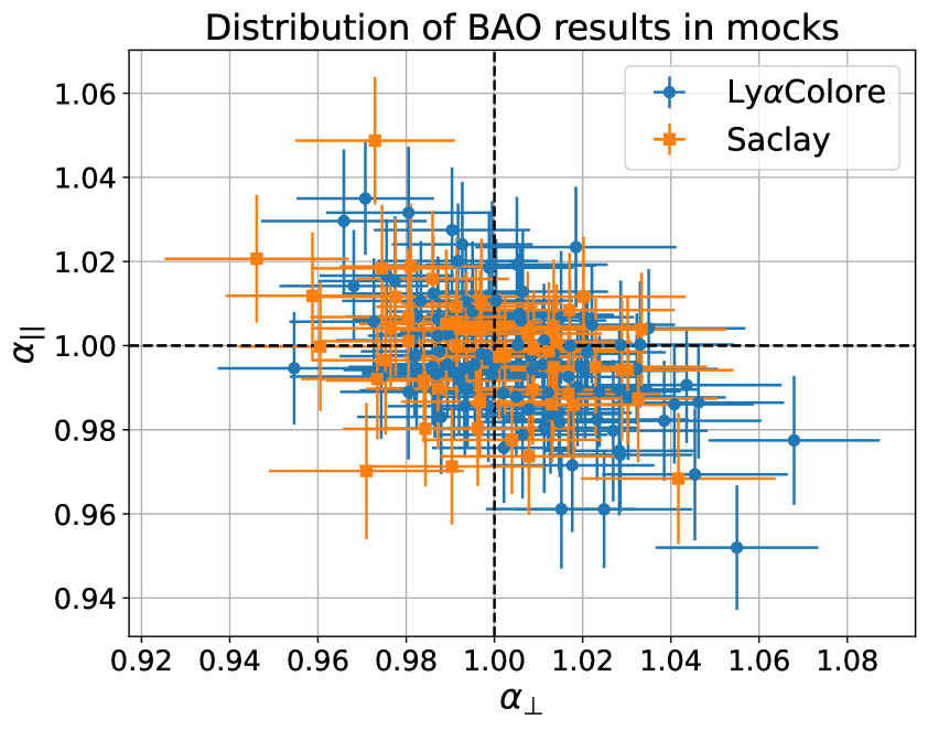
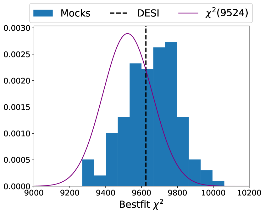
Figure 8: (left) Individual BAO measurements from 100 Ly$\alpha$CoLoRe (blue) and 50 Saclay (orange) mocks. These results are obtained using the iminuit minimizer. The black dashed lines at $\alpha_{||}=\alpha_{\bot}=1$ indicate the input mock cosmology. (right) Histogram of the best-fit $\chi^{2}$ statistic (blue), along with the expected $\chi^{2}$ distribution (purple line), and the best-fit $\chi^{2}$ value obtained from the real DESI data (black dashed line). The data value is consistent with both the distribution of mocks and the expected distribution. However, the distribution of mocks is systematically shifted to larger values compared to the expected $\chi^{2}$ distribution. We discuss this shift in Appendix A.

We next shift our focus to analysing the mocks individually and studying the statistics of the entire mock population. The individual BAO measurements from the 100 Ly$\alpha$CoLoRe and 50 Saclay mocks are shown in the left panel of Figure 8. They are scattered around the truth ($\alpha_{||}=\alpha_{\bot}=1$), with the two distributions of Ly$\alpha$CoLoRe and Saclay mocks showing similar variance. We have checked that the two populations are consistent with each other by first performing all the tests described below separately for Ly$\alpha$CoLoRe and Saclay mocks. As we found no indication of inconsistency, we combine the two sets of mocks and present the statistics of all 148 mock BAO measurements below.

The distribution of best-fit $\chi^{2}$ values is shown in the right panel of Figure 8, along with the best-fit $\chi^{2}$ value obtained from the DESI DR1 data. The expectation for mocks is to recover a $\chi^{2}$ distribution with $9540-16=9524$ degrees of freedom. For data, DESI2024-Ly$\alpha$ fit 17 parameters resulting in a slightly smaller $9523$ degrees of freedom. The $\chi^{2}$ value obtained from DESI DR1 (black dashed line) is consistent with both the distribution of mock values and the expected $\chi^{2}$ distribution. However, we find that the distribution of best-fit $\chi^{2}$ values in our mocks is somewhat larger than the expected value, having a mean and standard deviation of $9654\pm 148$. This shift to larger $\chi^{2}$ values is caused for the most part by the failure of our linear theory model to fit the correlation functions of the mocks across the entire range of scales we use. We demonstrate this using Monte Carlo simulations of correlation functions in Appendix A. This result is not surprising given that our mocks deviate from linear theory at small scales (quite significantly in the case of Ly$\alpha$CoLoRe mocks). The analysis of [35] had to use a significantly narrower range of $40<r<160$  $h^{-1}\text{Mpc}$ to obtain a good fit to correlation functions measured directly from the Ly$\alpha$CoLoRe transmitted flux boxes. We aim to stay as close as possible to the analysis on real DESI data, which means we use the extended $10<r<180$  $h^{-1}\text{Mpc}$ range. Therefore, we expect the linear theory model to not be able to accurately fit this entire range. Furthermore, the failure of the linear theory model extends to large scales due to the metal peaks present along the line-of-sight in our correlation functions, as these peaks represent the small-scale cross-correlation between Ly$\alpha$ flux (or quasars) and the individual metal absorbers (see Figures 3 and 4). Despite these failures of our model, we are still able to obtain unbiased measurements of the BAO peak position as shown above. Furthermore, while our goal here is to study BAO fits using a physical model, DESI2024-Ly$\alpha$ also tested modelling variations with added broadband polynomials which effectively marginalize over potential systematic effects caused by the failure of the model on small scales.

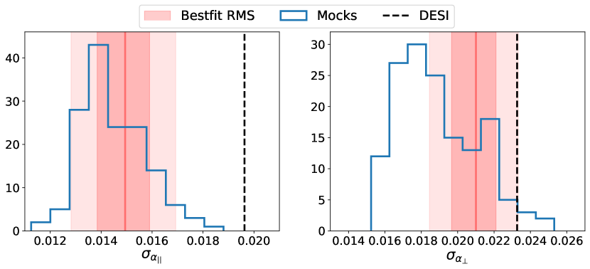
Figure 9: Distribution of uncertainties for the 150 BAO measurements from mocks. Uncertainties in $\alpha_{||}$ are shown in the left panel, and uncertainties in $\alpha_{\bot}$ are shown in the right panel. The red line and bars indicate the scatter of BAO best-fit measurements in the population of mocks, with the darker (lighter) region indicating the $68\%$ ($95\%$) credible region. This is consistent with the blue histogram, indicating the measured uncertainties are representative of the real uncertainty in these measurements. The dashed black lines indicate the uncertainties in the DESI DR1 Ly$\alpha$ BAO measurement.

Another important test that synthetic datasets allow us to perform is checking the recovered BAO uncertainties, $\sigma_{\alpha_{||}}$ and $\sigma_{\alpha_{\bot}}$, against the scatter of BAO best fits. Assuming Gaussian distributed results, if the covariance matrix estimation is unbiased and we correctly marginalize all nuisance parameters, we expect the two to be consistent with each other. We show the distribution of uncertainties on $\alpha_{||}$ and $\alpha_{\bot}$ in Figure 9, along with the RMS deviation of best-fit values (red line and bars). We find that the scatter of BAO best fits in mocks is broadly consistent with the reported uncertainties (red line is within the blue histogram). As we have a fairly limited number of mocks (150), this comparison is quite noisy as shown by the large uncertainties on the RMS deviation of best-fit values. We test our uncertainties more rigorously using the pull distributions below. In Figure 9, we also show the uncertainties obtained from DESI DR1 (black line). This appears to be quite an extreme result when compared to the mocks, with only $5$ mocks having a larger $\alpha_{\bot}$ uncertainty, and no mocks having an uncertainty as large as the data in $\alpha_{||}$. However, this difference can be explained by the fact that our mocks do not include the effect of BAO broadening due to non-linear evolution. We demonstrate this in Section 5 using Monte Carlo simulations.

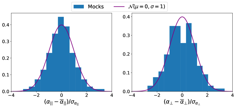
Figure 10: Distribution of normalized residuals in $\alpha_{||}$ (left) and $\alpha_{\bot}$ (right) from the set of 150 BAO measurements in mocks. The purple lines indicate the expected distributions, i.e. Gaussian with unit variance.

As a final test of the measured uncertainties, we show the pull distributions for $\alpha_{||}$ and $\alpha_{\bot}$ in Figure 10. These are obtained by subtracting the mean value of mock BAO best fits from each individual result, and dividing by the measured uncertainty (i.e. $[\alpha-\bar{\alpha}]/\sigma_{\alpha}$). We can test whether our measured uncertainties are representative of the real uncertainty by checking if the standard deviations of the pull distributions are consistent with unity. Figure 10 includes a unit variance Gaussian for comparison. The standard deviations of these distributions are $1.02\pm 0.07$ for $\Delta\alpha_{||}/\sigma_{\alpha_{||}}$, and $1.11\pm 0.06$ for $\Delta\alpha_{\bot}/\sigma_{\alpha_{\bot}}$, with uncertainties obtained through bootstrap. This test assumes both that the distribution of BAO best-fits is Gaussian (through the use of the standard deviation), and that the posterior distributions of individual measurements can be approximated as Gaussian (because we use Gaussian uncertainties from iminuit). Neither of these were true for previous Ly$\alpha$ forest BAO analyses [e.g. 28, 27, 31]. However, in the case of DESI DR1 mocks, Figure 10 shows that the Gaussian assumption works very well for $\alpha_{||}$, and moderately so for $\alpha_{\bot}$. If instead of the standard deviation, we use the $68\%$ credible region, we obtain $0.93\pm 0.09$ for $\Delta\alpha_{||}/\sigma_{\alpha_{||}}$, and $1.08\pm 0.09$ for $\Delta\alpha_{\bot}/\sigma_{\alpha_{\bot}}$. This does not rely on the first assumption of Gaussian distributed best-fits, and therefore confirms both that the second assumption is justified (we can approximate posterior distributions as Gaussian), and that the uncertainties are well estimated using our framework. We end by noting that while this analysis validates our BAO uncertainties, it only does so at the $\sim 9\%$ level, which is expected given the relatively small number of mocks we have (150).

4.3 Covariance matrix tests

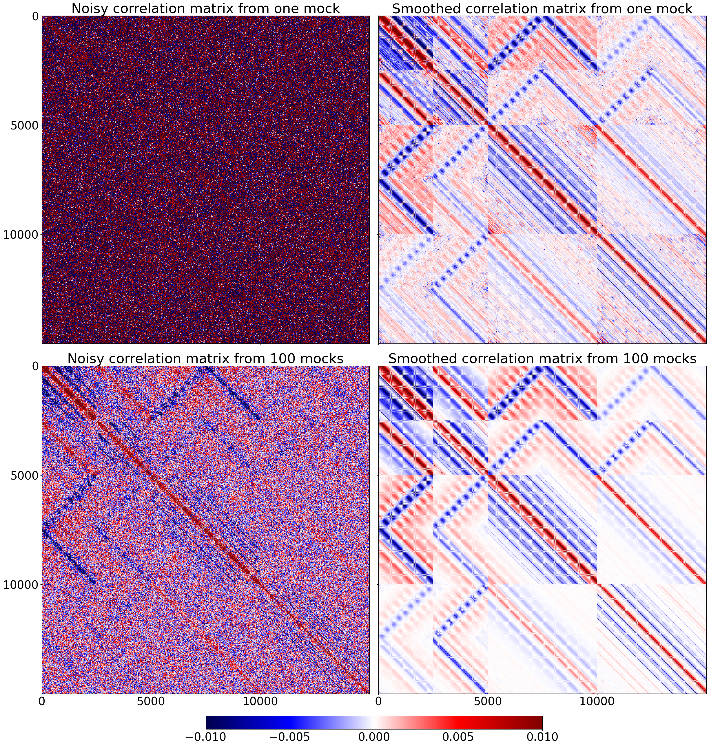
Figure 11: Global correlation matrices of all four Ly$\alpha$ forest correlation functions. The top row shows correlation matrices computed from one Ly$\alpha$CoLoRe mock, while the bottom row shows the mean correlation matrices computed from all 100 Ly$\alpha$CoLoRe mocks. We plot the initial noisy estimates of the correlation matrix in the left column, while the smoothed versions are shown in the right column. In each panel, the global correlation matrix is made up of the individual auto-correlation matrices for each of the four correlation functions in order: Ly$\alpha$(A)$\times$Ly$\alpha$(A), Ly$\alpha$(A)$\times$Ly$\alpha$(B), Ly$\alpha$(A)$\times$QSO, Ly$\alpha$(B)$\times$QSO (diagonal blocks), and all the possible cross-correlation matrices (off-diagonal blocks). Note that the range of the colour scale is 100 times smaller than in Figure 5.

The DESI DR1 Ly$\alpha$ BAO analysis uses one global covariance matrix for all four Ly$\alpha$ correlation functions. This is because, for this data set, the cross-covariance between the different correlation functions cannot be ignored as was done with previous BOSS and eBOSS analyses. This is discussed in detail in DESI2024-Ly$\alpha$. The result of needing to account for the cross-covariance is that we now need to estimate a $15000\times 15000$ covariance matrix. Due to computational and storage constraints, we are limited to a sample of 150 mock data sets, which means we cannot use mocks to directly estimate our covariance matrix. Therefore, for this work, we rely on the same method used in previous Ly$\alpha$ BAO analyses to estimate our covariance matrices [26, 31]. As described in Section 3.3, this involves first computing a noisy estimate from the $1028$ correlation function measurements in $250\times 250\;(h^{-1}\mathrm{Mpc})^{2}$ patches on the sky, and then smoothing this noisy estimate to obtain our measurement of the covariance matrix. This process was used to estimate the data covariance matrix in DESI2024-Ly$\alpha$, and the covariance matrices for each of our mocks here. The method has also been tested against the much slower method of computing the Gaussian covariance using the Wick approximation, and the two were found to produce consistent results [31]. In this section, we wish to use the population of mocks to study how well this method works for individual mocks, and to test the impact on BAO measurements.

In Section 3.3 we also introduced the covariance matrix estimates from the stack of mocks (which were used to obtain the results in Section 4.1). These estimates use $\sim 100$k samples for Ly$\alpha$CoLoRe and $\sim 50$k samples for Saclay instead of the $1028$ we have in individual mocks. Therefore, they represent much better estimates of the covariance matrices of these mock data sets. We show the normalized global covariance matrices (i.e. correlation matrices) from one Ly$\alpha$CoLoRe mock and from the stack of 100 Ly$\alpha$CoLoRe mocks in Figure 11. Each of these global matrices contains the individual auto-correlation matrices (diagonal blocks) for the four correlation functions in order: Ly$\alpha$(A)$\times$Ly$\alpha$(A), Ly$\alpha$(A)$\times$Ly$\alpha$(B), Ly$\alpha$(A)$\times$QSO, Ly$\alpha$(B)$\times$QSO. The two auto-correlation functions have covariance matrices of size $2500\times 2500$, while the two cross-correlation functions have covariance matrices of size $5000\times 5000$. Off-diagonal blocks represent the cross-covariance matrices between different correlation functions. The strongest of these is the cross-covariance between Ly$\alpha$(A)$\times$Ly$\alpha$(A) and Ly$\alpha$(A)$\times$QSO (Figure 6).

From Figure 11 we can see that the initial estimate of the covariance matrix in individual mocks (top left) shows no clear features away from the diagonal due to noise. We can start to see the features of the correlation matrix when looking at the initial estimate from the stack of mocks (bottom left) due to the much larger sample size used to compute it. However, this estimate is still fairly noisy, which is why we also apply the smoothing procedure in this case. The two panels on the right show the smoothed correlation matrices from one mock (top) and from the stack of mocks (bottom). These two show that the smoothed covariance matrix from the stack of correlation functions is remarkably similar to the smoothed covariance estimated from individual mocks. This consistency is better illustrated in Figure 12, which shows the line-of-sight components of the covariance matrix for the Ly$\alpha$ auto-correlations and the Ly$\alpha$-QSO cross-correlation. We focus on correlations between line-of-sight bins as they are the most important part of the covariance matrix (see Section 3.3).

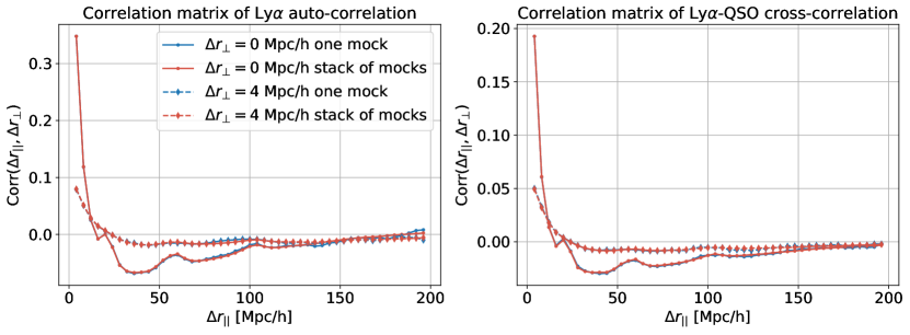
Figure 12: The smoothed normalized covariance matrix (correlation matrix) for the Ly$\alpha$ auto-correlation (left) and the Ly$\alpha$-QSO cross-correlation (right). We compare the smoothed correlation matrix as a function of line-of-sight separation for one Ly$\alpha$CoLoRe mock versus the stack of 100 Ly$\alpha$CoLoRe mocks. This figure shows that the smoothing applied to the very noisy estimate of the covariance from one mock leads to a correlation structure that is remarkably similar to the smoothed correlation matrix from the stack of mocks.

As the initial estimates of the covariance matrix in individual mocks are dominated by noise, we wish to test our method for estimating and smoothing covariance matrices by comparing the results obtained in Section 4.2 with results obtained with the more robust covariance matrix from the stack of mocks. To do this, we build new covariance matrices from the correlation matrix estimate of the stacks of mocks and the variance estimates in each mock:

$$C_{MN}^{test}=(C_{MM}C_{NN})^{1/2}Corr_{MN}^{\mathrm{stack}},$$ (4.1)

where $Corr_{MN}^{\mathrm{stack}}$ is the correlation matrix estimate from the stack of mocks (given by Equation 3.12), and $C_{MN}^{test}$ are our new test covariance matrices for each mock. As two of the mocks were already using these covariance matrices (see Section 3.3), we discard them from the analysis in this section and work with the remaining 148 mocks.

We then fit the mocks using these new estimates and compare the BAO results with the previous results from Section 4.2. The difference between the best-fit $\alpha_{||}$ and $\alpha_{\bot}$ of each mock is shown in Figure 13. The shifts in the BAO position are randomly distributed with very small RMS compared to the uncertainty of the DESI DR1 constraints. We measure the RMS of $\Delta\alpha_{||}$ to be $0.0012\pm 0.0001$, and the RMS of $\Delta\alpha_{\bot}$ to be $0.0014\pm 0.0002$. These represent less than a tenth of the DESI DR1 uncertainty. We also compared the uncertainties in $\alpha_{||}$ and $\alpha_{\bot}$ obtained with the two covariance matrix estimates, and we found the changes are randomly distributed as well, and of the order of $\sim 1\%$ of the DESI DR1 uncertainty. This means the two estimates of the covariance matrix produce consistent BAO results.

On the other hand, when comparing the best-fit $\chi^{2}$ values of the two populations, we found a small systematic shift to smaller $\chi^{2}$ values when using the correlation matrix estimated from the stack of mocks. The mean and RMS of the shift are roughly $\Delta\chi^{2}=-30\pm 10$, with $147$ out of $148$ mocks having an improved (smaller) $\chi^{2}$. This shift is too small to explain the results in Figure 8, but indicates that the noisy estimate of the covariance matrix has a small but significant impact on the quality of the model fits.

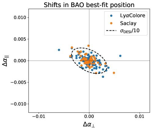
Figure 13: Shifts in the BAO best-fit positions from mocks when using the correlation matrix estimated from the stack of all mocks versus the correlation matrix estimated from each individual mock. The stack of mocks provides a much larger sample ($100$k for Ly$\alpha$CoLoRe, and $50$k for Saclay) to estimate the covariance matrix. As shown here, using these improved estimates leads to small random shifts in the measured BAO position. However, these are unbiased and much smaller than the DESI DR1 BAO uncertainty. The black dashed contour indicates one-tenth of the DESI DR1 uncertainty.

4.4 Impact of redshift errors

In line with previous analyses [e.g. 71, 31], we have so far only considered the impact of redshift errors through their smoothing effect on the Ly$\alpha$-QSO cross-correlation. The redshift errors used here were generated using a Gaussian distribution with dispersion $\sigma_{z}=400\ \text{km/s}$ ( Section 2.3). See [72] for a comparison between redshift errors measured in DESI mocks versus DESI data. [45] found that redshift errors can also introduce spurious correlations in both the Ly$\alpha$ auto- and its cross-correlation with quasars. These spurious correlations appear due to the smearing of emission lines in the forest region, leading to errors in the fitted continuum of each forest. These errors do not average out because quasars are not uniformly distributed (i.e. they are clustered). Therefore, the two ingredients that contribute to these spurious correlations are the smearing of emission lines in the forest regions and the quasar auto-correlation function [45].

In this section, we wish to study the impact of spurious correlations caused by redshift errors on BAO measurements. We did not include this effect in our baseline mocks because we know based on [45] that it is more extreme in our mocks than in reality. This has to do with both ingredients that give rise to this effect. Firstly, the quasar auto-correlation in our mocks is significantly larger on small scales compared to realistic simulations (see Figure 6 of [45]). This is because we use the log-normal approximation to draw quasar position in both Ly$\alpha$CoLoRe and Saclay mocks. Secondly, in our mocks, the smearing of emission lines in the forest region is completely random, but in reality, this smearing is likely smaller because we use emission lines (on the red side of the Ly$\alpha$ line) to measure the redshift. This means that even if the measured quasar redshift has some error relative to the systemic redshift, it is likely better at predicting the position of emission lines in the forest region than the systemic redshift. Therefore, we decided not to include this effect in our baseline mocks. Nevertheless, we study its impact on BAO measurements with the caveat that our results likely overestimate it.

We show the impact of the spurious correlations on stacks of correlation functions from Ly$\alpha$CoLoRe and Saclay mocks in Figure 14. As shown by [45], these have an impact mostly limited to the line-of-sight wedge, but that extends to very large separations (even larger than the BAO scale). From Figure 14, this appears most pronounced in the roughly $50-80$  $h^{-1}\text{Mpc}$ interval where the blended SiII(1190) and SiII(1193) metal peak is located, and in the roughly $90-110$  $h^{-1}\text{Mpc}$ interval that overlaps the location of the BAO peak.

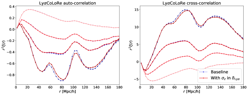
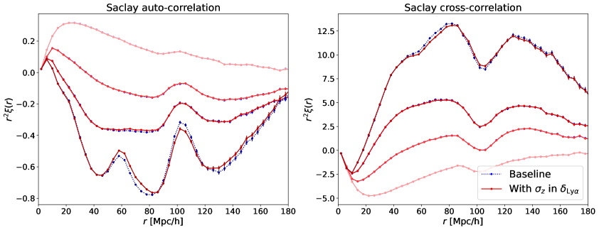
Figure 14: Stacked correlation functions compressed into $\mu$ wedges (points with error bars and lines connecting them), with lighter colours indicating smaller $\mu$ values, and darker colours indicating larger $\mu$ values. The top panels show stacked correlations from 100 Ly$\alpha$CoLoRe mocks, while the bottom panels show stacked correlations from 50 Saclay mocks. The left panels show Ly$\alpha$ auto-correlations, while the right panels show Ly$\alpha$-QSO cross-correlations. In our baseline mocks (blue), redshift errors only have a smoothing effect on the cross-correlation. On the other hand, red correlations come from mocks where redshift errors also affect the fitted quasar continuum by smearing emission lines in the forest region.

The presence of these spurious correlations in the BAO region means there could be systematic errors in the measured BAO signal. To check for this, we perform two types of tests. First, we fit the BAO peak position using the stacked correlation functions, similarly to Section 4.1, and check if the results are still within the threshold we set above ($1/3$ of the DESI DR1 Ly$\alpha$ BAO uncertainty). We show these results in Figure 15. While the measurements are slightly different than the results presented in Figure 7, they are both still within the threshold (dashed black line). This indicates the spurious correlations do have an impact on BAO measurements, but the impact is very small.

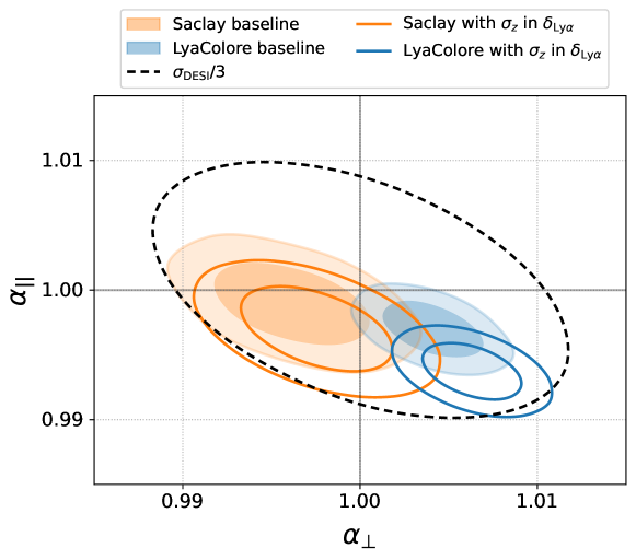
Figure 15: Similar to Figure 7, but now including results from mocks where redshift errors affect the fitted quasar continuum. These redshift errors lead to spurious correlations in both the auto- and cross-correlation as shown in Figure 14. This result indicates that while the spurious correlations have an impact on BAO measurements, this is very small ($<0.2\%$). Importantly, the mock measurements are still within the threshold of $1/3$ of the DESI DR1 BAO uncertainty (blue and orange contours are within the dashed black line).

Secondly, we attempt to quantify the impact on BAO measurements by again fitting all of the mocks (now including spurious correlations due to redshift errors), and computing the mean shift in the BAO position. We find that there is indeed a shift in the BAO positions, which for Ly$\alpha$CoLoRe mocks we measure to be $\Delta\alpha_{||}=-0.0032\pm 0.0004,\;\Delta\alpha_{\bot}=0.0027\pm 0.0004$, and for Saclay mocks we measure as $\Delta\alpha_{||}=-0.0018\pm 0.0007,\;\Delta\alpha_{\bot}=0.0010\pm 0.0007$. The quoted uncertainties are derived through bootstrap of the BAO best-fit positions (i.e., these measurements are based on the best-fit BAO positions and not on the posterior distributions).

For this test, it is also useful to re-parameterize our BAO coordinates, into the isotropic BAO component, and the anisotropic component which captures the Alcock-Paczyński (AP) information. Following [73], we define the isotropic component as $\alpha=\sqrt{\alpha_{\bot}\alpha_{||}}$, and the Alcock-Paczyński direction as $\phi=\alpha_{\bot}/\alpha_{||}$. When working in the $\phi,\alpha$ coordinates, it becomes clear that the systematic shift due to spurious correlations is largely in the Alcock-Paczyński direction, with $\Delta\phi=0.0061\pm 0.0008$ for Ly$\alpha$CoLoRe mocks and $\Delta\phi=0.0029\pm 0.0013$ for Saclay mocks. The Ly$\alpha$CoLoRe measured bias is very significant ($\sim 8\sigma$) and is about double in magnitude compared to the one measured from Saclay mocks, which is only $\sim 2.2\sigma$ from $0$. On the other hand, the isotropic BAO measurement does not show the same significant bias, with $\Delta\alpha=-0.0006\pm 0.0004$ for Ly$\alpha$CoLoRe mocks, and $\Delta\alpha=-0.0008\pm 0.0008$ for Saclay mocks. The two measurements are now consistent and within $2\sigma$ of $0$. For comparison, the DESI DR1 Ly$\alpha$ BAO uncertainties, are $\sim 0.04$ in $\phi$ and $\sim 0.016$ in $\alpha$.

As discussed in Section 2.1, Saclay mocks have more realistic quasar clustering when compared to Ly$\alpha$CoLoRe mocks, in which the small-scale quasar auto-correlation is much larger than measured in simulations and real data. This explains why the shift in the AP direction is roughly double in Ly$\alpha$CoLoRe mocks compared to Saclay mocks. However, the isotropic BAO shifts are consistent with each other and not significant (below $2\sigma$). Therefore, using our sample of mocks, we have strong indications of a bias in the AP direction, but the isotropic BAO direction is not significantly biased at the level tested. Nevertheless, it is clear that these systematic shifts are small compared to the DESI DR1 BAO uncertainties. Taking the Saclay results as the more realistic ones, the shifts are less than a tenth of $\sigma_{\mathrm{DESI}}$ in both directions and as discussed above, our analysis likely overestimates the impact of this effect.

While the spurious correlations studied here have minimal impact on the recovered BAO peak position, they have a much larger impact on other nuisance parameters. The systematic biases are not relevant for BAO, because DESI2024-Ly$\alpha$ found that none of the nuisance parameters are correlated with $\alpha_{||}$ or $\alpha_{\bot}$. However, we mention the most important of these shifts here for completeness. We report all systematic shifts relative to their DESI DR1 uncertainty. We find that both the Ly$\alpha$ bias ($b_{\mathrm{Ly}\alpha}$) and RSD ($\beta_{\mathrm{Ly}\alpha}$) parameters are shifted to lower values by $\sim 1\sigma$ in Ly$\alpha$CoLoRe mocks, and $\sim 0.5\sigma$ in Saclay mocks. The HCD bias ($b_{\mathrm{HCD}}$) and typical length scale ($L_{\mathrm{HCD}}$) are both shifted to larger values by $\sim 1\sigma$. The most affected parameter is the bias of the SiII$(1190)$ line which is shifted by $\sim 2\sigma$ to more negative values. Given the position of this metal peak is at $\sim 60$ $h^{-1}\text{Mpc}$, this shift indicates that the metal model is fitting the spurious correlation observed in Figure 14 at the same scales. That is also true for the SiII$(1260)$ peak at $\sim 103$ $h^{-1}\text{Mpc}$, but its bias parameter only displays a $\sim 0.5\sigma$ shift to larger (less negative) values. As the spurious correlations display similar patterns to the metal contamination (they appear as peaks and troughs along the line-of-sight only, and rapidly decay across the line of sight), it is not surprising that the metal models also fit these features. However, given our results here, creating a model for these spurious correlations so they can be properly marginalized should be one of the top priorities for future Ly$\alpha$ forest analyses.

5 Discussion

The results presented in this publication were used to validate the DESI DR1 Ly$\alpha$ forest BAO measurement from DESI2024-Ly$\alpha$. We performed the same analysis as DESI2024-Ly$\alpha$ on a set of 150 mock data sets that include the major Ly$\alpha$ forest contaminants and found no significant systematic biases in the recovered BAO peak position. We also found that the BAO uncertainties measured in mocks are consistent with the spread of BAO best-fit measurements and that our method for estimating the covariance matrix leads to consistent results when compared to the improved estimate from a large population of mocks. In this section, we wish to discuss the applicability of our results given the limitations we have in terms of our synthetic Ly$\alpha$ forest data sets.

The largest limitation with the current generation of Ly$\alpha$ forest mocks is that they are based on the log-normal approximation. The Ly$\alpha$ forest mostly probes linear and mildly non-linear regimes due to the self-censoring of large overdensities which quickly absorb all Ly$\alpha$ flux. Furthermore, DESI measurements of the Ly$\alpha$ forest are limited to redshifts $z>1.95$, when the matter in the Universe was still linear on much smaller scales than today [65, 74]. This means that modelling the large scales considered in Ly$\alpha$ forest BAO analyses only requires small deviations from linear theory [74, 75]. Therefore, log-normal mocks can be very useful, especially when studying the Ly$\alpha$ auto-correlation, where the main limitation only comes from the fact that these mocks do not include the BAO broadening due to non-linear evolution (see discussion below). When modelling real data, small-scale non-linearities are usually modelled using an ad-hoc equation tuned from hydrodynamical simulations [65]. However, we found that the presence or absence of this model has no impact on current BAO measurements, both with real data (DESI2024-Ly$\alpha$), and with the mocks here.

While the log-normal approximation works well for the Ly$\alpha$ forest on large scales, it fails to correctly simulate the quasar distribution, especially on small scales, which could impact measurements of the Ly$\alpha$-QSO cross-correlation. For the mocks used in this work, this is a larger issue in Ly$\alpha$CoLoRe mocks, which greatly overpredict the small-scale quasar clustering [34, 45]. However, this is less of a problem in Saclay mocks, because they draw quasars from a simulated quasar density field instead of the matter field, which leads to more accurate small-scale QSO clustering [36]. This is why we have compared the results from Ly$\alpha$CoLoRe and Saclay mocks throughout this article. The fact that the main results in Sections 4.1 and 4.2 do not show significant discrepancies between the two types of mocks indicates that this effect does not have a large impact on BAO measurements. The only place where we have found discrepant results was in Section 4.4, where we know the spurious correlations due to redshift errors are directly related to the strength of the quasar clustering [45].

As noted above, the most relevant effect for BAO that is not modelled in our mocks is the broadening due to non-linear evolution. To understand the impact of this effect, we performed the test presented in Figure 16. We used the covariance matrix measured by DESI2024-Ly$\alpha$ from DESI DR1 to create two populations of Monte Carlo simulations of our correlation functions following the method in Appendix A. The first population is based on the best-fit model to DESI DR1, which includes the BAO broadening effect. This broadening is modelled by adding Gaussian smoothing to the peak component of the template power spectrum following [22]. The second population uses the same model but without the BAO broadening. We find that this second population matches very well the distribution of BAO uncertainties we measure from our mocks (Figure 16), while the first is shifted to larger uncertainties that match the actual measurement from DESI DR1. Therefore, at the level of DESI DR1, BAO broadening leads to a $\sim 50\%$ increase in uncertainty for $\alpha_{||}$, and $\sim 25\%$ for $\alpha_{\bot}$.

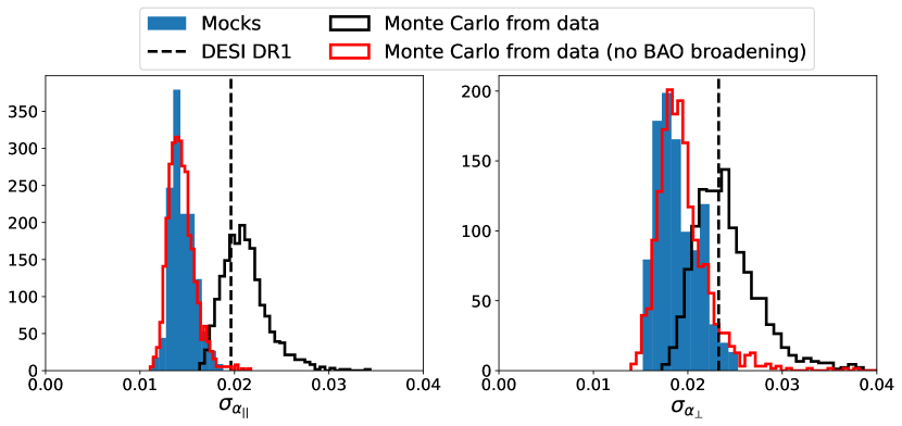
Figure 16: Distribution of BAO uncertainties for the mock measurements (blue) versus two populations of Monte Carlo (MC) simulated correlation functions. The MC simulations are based on the best-fit model and covariance matrix measured from DESI DR1. The distribution in black uses the model that was used to fit the data, which includes BAO broadening due to non-linear evolution, while the distribution in red uses the same model but without the BAO broadening effect. The vertical dashed lines represent the uncertainties measured from DESI DR1. This shows that the BAO broadening effect can fully explain the difference between the BAO uncertainties measured in mocks versus data.

The model for this BAO broadening effect is based on Lagrangian perturbation theory [76], and is described in detail in [22]. It has been used in all Ly$\alpha$ forest BAO analyses to date. Recently, [75] used Ly$\alpha$ forest mocks based on N-body simulations to show that this model fits the BAO broadening effect very well. Therefore, while this feature is absent from our mocks, it is well understood and accounted for in Ly$\alpha$ forest BAO analyses. Furthermore, Figure 16 shows that the DESI DR1 uncertainties are consistent with the population of MC mocks produced from the model with BAO broadening (validated in [75]) and the covariance matrix (validated here). Nevertheless, our results here serve as a strong basis for moving towards more realistic mocks in future Ly$\alpha$ forest analyses [e.g., 77, 78, 75].

Contamination due to metal absorption in the forest region is added both to our mocks and also modelled at the level of the correlation function. However, current-generation mocks have a relatively simplistic treatment for this metal absorption. We use Ly$\alpha$ flux skewers and re-scale them such that resulting mocks reproduce the metal biases measured from real data (see Section 2.4). This has two main weaknesses. The first was exposed in Section 4.4, where we found that some of the metal biases are systematically shifted because of spurious correlations due to redshift errors. This means the metal tuning process cannot replicate realistic metal contamination unless we are able to properly model these spurious correlations. The second weakness comes from the fact that real metal contamination is associated with the circum-galactic and intra-galactic medium, rather than the IGM [79]. This means our use of the Ly$\alpha$ flux skewers which trace the IGM only provides a very rough approximation for the metal contamination. A more realistic approach would be to draw metal lines from the peaks of the matter field, similar to how quasars and DLAs are drawn [35]. In terms of BAO analyses, metal contamination is most relevant due to the SiII$(1260)$ line which leads to the metal peak observed at $\sim 103$ $h^{-1}\text{Mpc}$, close to where the BAO peak is located. However, we find that our model is able to tell the two apart both in the mocks here and in the DESI DR1 data (DESI2024-Ly$\alpha$). Neither $\alpha_{||}$ nor $\alpha_{\bot}$ is correlated with the bias parameter of this metal line, indicating that our measurement of the BAO position is not sensitive to differences between how this metal line is added in mocks versus how it appears in real data.

While our mocks contain the major Ly$\alpha$ forest contaminants, there are a few less important effects that appear in real data but are not included here. These are:

• CIV contamination: The auto-correlation of CIV absorption in the forest region has been modelled in previous Ly$\alpha$ forest BAO analyses, but not detected at a significant level [31, 1].

• Transverse proximity effect: We expect quasar radiation to have a significant impact on their surrounding environment, by increasing the ionization rate. This effect appears on small scales in the Ly$\alpha$-QSO cross-correlation and has been modelled in previous analyses using a simple model proposed by [71].

• Correlated sky residuals: Spectra from fibers in the same DESI petal [80] have correlated noise introduced by the data reduction pipeline. This has been studied in [81], and a simple model was proposed that can accurately account for this contamination. This model is included in the analysis of DESI2024-Ly$\alpha$.

• UV background fluctuations: Fluctuations in the ionizing UV background can make the Ly$\alpha$ bias and RSD parameters scale dependent [82, 83]. This has been modelled following [83] in previous Ly$\alpha$ forest BAO analyses, but not detected at a significant level.

We note that none of these effects impact BAO measurements, and all have been tested as part of the blinded analysis performed in DESI2024-Ly$\alpha$.

None of the limitations discussed here significantly affect our ability to use the mocks presented in this work to validate the DESI DR1 Ly$\alpha$ BAO measurement. However, based on our results here, we have identified a few priorities for improving the next generation of synthetic data sets. These include going beyond the log-normal approximation in order to simulate non-linear broadening of the BAO peak and realistic quasar clustering down to small scales [e.g., 77, 78, 75], improving the realism of how metal contamination is added in mocks [e.g., 35], and generating a much larger set of mocks to improve our ability to study covariance matrix estimates and validate our uncertainties with improved precision.

6 Summary

The first year of data from the Dark Energy Spectroscopic Instrument (DESI) contains the largest set of quasar spectra ever observed. Lyman-$\alpha$ (Ly$\alpha$) forests measured from these spectra were used by DESI2024-Ly$\alpha$ to measure Baryon Acoustic Oscillations (BAO) at an effective redshift $z=2.33$ with unprecedented precision. In this work, we use synthetic data sets (mocks) to perform the analysis validation for this DESI data release 1 (DR1) Ly$\alpha$ BAO measurement.

We use a set of 150 mocks generated from Gaussian random fields with quasar positions and the Ly$\alpha$ transmitted flux field inferred from its log-normal transformation. 100 of these were generated using Ly$\alpha$CoLoRe [34, 35], and 50 were generated using the Saclay framework described in [36]. These initial mocks were then used to simulate DESI DR1 quasar catalogues, and generate realistic DESI spectra following [37]. The spectra include the major Ly$\alpha$ forest contaminants, such as metal absorption, damped Ly$\alpha$ systems (DLAs), broad absorption lines (BALs), and redshift errors. We describe the process of creating the mock data sets in Section 2.

We present our results in Section 4, where we perform two types of studies. First, we stack the correlation functions from all mocks to obtain very high statistics measurements of the Ly$\alpha$ correlations and use these to check for potential systematic biases affecting the measurement of the BAO position. The results of this study are presented in Figure 7, which shows that using our mocks we are able to obtain unbiased measurements of the BAO parameters $\alpha_{||}$ and $\alpha_{\bot}$. Secondly, we analyze each mock individually and study the statistics of the resulting population of BAO fits in Section 4.2. We find that mock BAO constraints are randomly scattered around the truth (Figure 8), with an RMS that roughly matches the measured uncertainties on $\alpha_{||}$ and $\alpha_{\bot}$ (Figure 9). Finally, we use the pull distribution shown in Figure 10 to validate the BAO uncertainties at the $\sim 9\%$ level. However, as our mocks do not include the effect of BAO broadening due to non-linear evolution, the uncertainties we measure here are significantly tighter than in real data (see Section 5).

In our baseline analysis, each mock has its own estimate of the covariance matrix. However, these are very noisy as they are based on the covariance of correlations computed in $1028$ patches on the sky (see Section 3.3 and Figure 11). In Section 4.3, we test these noisy estimates by performing another analysis of the mock population using the normalized covariance (correlation matrix) estimated from the set of all mocks, which is much less noisy. We find that the choice of covariance matrix estimate does not have a significant impact on BAO constraints.

We test the impact of redshift errors in Section 4.4, in the scenario where they are allowed to impact the continuum fitting process following [45]. Redshift errors give rise to smearing of emission lines in the forest region, and due to the clustering of quasars, these continuum errors lead to spurious correlations in both the Ly$\alpha$ auto and its cross-correlation with quasars [45]. We find that these spurious correlations can produce a small but detectable systematic bias in the measured BAO peak position. This bias was found to only affect the Alcock-Paczynski direction and not the isotropic BAO measurement. However, even the Alcock-Paczynski BAO measurement was only biased by less than a tenth of the DESI DR1 uncertainty. While our results suggest this effect is not significant for DESI DR1, they do emphasize the need to model these spurious correlations, so future analyses can correctly marginalize them.

Finally, in Section 5 we discuss the applicability and limitations of the results presented here. The main limitations include the fact that we use log-normal mocks, which do not include the effect of BAO broadening and overpredict the small-scale quasar clustering. However, the large scales used for BAO analyses are not significantly impacted by this [75], and Figure 16 combined with tests performed in [1, 75] show that we understand and can accurately model the effect of BAO broadening in real data. Nevertheless, we expect that the work and results presented here will motivate further development of more realistic mock data sets of the Ly$\alpha$ forest.

The work presented here was used to validate the DESI DR1 Ly$\alpha$ forest BAO analysis, and motivate decisions made during that analysis (DESI2024-Ly$\alpha$). This led to the tightest BAO constraints from large-scale structure at redshifts $z>2$. DESI2024-Ly$\alpha$ measured the expansion rate at redshift $z=2.33$ with $2\%$ precision, and the transverse comoving distance to that redshift with $2.4\%$ precision.

7 Data Availability

The data used in this work will be made public as part of DESI Data Release 1 (details in https://data.desi.lbl.gov/doc/releases/)

Appendix A Tests with Monte Carlo simulations

To gain further insight into our results from Section 4.2, we used populations of Monte Carlo (MC) simulations of our correlation functions following [63]. We start with the covariance matrix measured from the stack of 100 Ly$\alpha$CoLoRe mocks and re-scaled to match the variance of one mock (multiplied by 100). We have also performed this test using the covariance matrix of one of the mocks and found similar results. Given a covariance matrix $C$ and correlation function $\xi$, we generate samples from the multivariate normal distribution with mean $\xi$ and covariance $C$. These samples are given by:

$$\tilde{\xi}=\xi+A\vec{y},$$ (A.1)

where the matrix $A$ is given by the Cholesky decomposition $C=AA^{T}$, $\vec{y}$ is a vector of N independent standard normal variates, and N is the size of C. These MC simulations of the correlation function are then fit using the same model from Section 3.4.

We generated two populations of MC simulations for our test. The first was created starting with the vector $\xi$ given by the stacked correlation functions from 100 Ly$\alpha$CoLoRe mocks, $\xi_{\mathrm{stack}}$. The second was created starting from the best-fit model to the stack of 100 Ly$\alpha$CoLoRe mocks, $\xi(\vec{\theta}_{\mathrm{best}})$, where $\vec{\theta}_{\mathrm{best}}$ represents the best-fit parameters. The two populations are then fit with the same model, and their resulting best-fit $\chi^{2}$ distributions are shown in Figure 17.

We find that the population based on the best-fit model matches the expected $\chi^{2}$ distribution with $9540-16=9524$ degrees of freedom very well. On the other hand, the population created from the stacked correlation functions is shifted to larger $\chi^{2}$ values and matches the observed $\chi^{2}$ distribution of our mocks. The covariance matrix used for these tests is correct by construction (i.e. the noise was generated with this covariance), and therefore, deviations from the expected $\chi^{2}$ distribution are caused by the inability of the model to fit the input $\xi$. This shows that the shift in the $\chi^{2}$ distribution measured from mocks is caused by our model failing to fit the measured correlation functions across the entire range of scales considered here ($10<r<180$ $h^{-1}\text{Mpc}$). We discuss this further in Section 4.2.

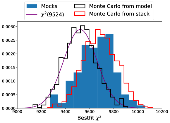
Figure 17: Histograms of the best-fit $\chi^{2}$ statistic. We compare the distribution measured from mocks (blue), with two distributions obtained from Monte Carlo (MC) simulations of the correlation function. The first set of MC simulations was generated based on the stack of measured Ly$\alpha$CoLoRe correlations in mocks (red), while the second was generated based on the best-fit model to the stack of 100 Ly$\alpha$CoLoRe mocks (black). The distribution of MC simulations based on the model is consistent with the expected $\chi^{2}$ distribution with $9540-16=9524$ degrees of freedom, while the other two distributions are shifted to larger $\chi^{2}$ values. This indicates that the shift in mock best-fit $\chi^{2}$ values is caused by the model failing to accurately fit the mock correlation functions.

Appendix B Tests of the fiducial cosmology

In the DESI DR1 BAO analysis, a fiducial cosmology based on the Planck 2018 results [41] is used to transform redshifts and angles to co-moving separations and as a template for the model. Here, we wish to validate that our constraints on $D_{\rm H}/r_{\rm d}$ and $D_{\rm M}/r_{\rm d}$ are independent of our choice of fiducial cosmology. To do this, we use a set of 20 Ly$\alpha$CoLoRe DESI Y5 mocks, created using the method described in Section 2, but mirroring the footprint and exposure time (4000s) of the expected DESI Y5 survey. For simplicity, we use mocks that do not contain any of the contaminants discussed above (e.g., metal absorption, HCDs, etc.), but that do go through the same continuum fitting procedure described in section 3.1. We only use the Ly$\alpha$(A)$\times$Ly$\alpha$(A) and Ly$\alpha$(A)$\times$QSO correlations for this test.

To perform this test we use five cosmologies: Planck 2018 results [Column 5 of Table 2 in 41], and four alternative cosmologies. Note that these are all different from the true cosmology used to create the Ly$\alpha$CoLoRe mocks used here (see Section 2.1). We highlight this by showing the truth (as crosses) in our results in Figures 18 and 19. In the first two of the four alternative cosmologies, we fix the sound horizon $r_{\rm d}$ and physical matter density $\Omega_{\rm m}h^{2}$ and vary $\Omega_{\rm m}$ and $h$ to the values given in Table 3. By fixing the sound horizon and physical matter density, which are both very well constrained from CMB anisotropies, we ensure the shape of our template power spectrum does not change. Thus we test the assumption that our BAO constraints are independent of the cosmology we use to make our coordinate transformation.

In the second set of alternative cosmologies, we instead fix $\Omega_{\rm m}$, while varying the values of $\Omega_{b}h^{2}$, $\Omega_{c}h^{2}$ and $h$. This changes $r_{\rm d}$ and $\Omega_{\rm m}h^{2}$, and therefore the shape of the template matter power spectrum, without affecting the coordinate transformation. The relevant values for this set are also given in Table 3. We choose values of $h=0.6472$ and $0.70$, which produces an $\pm$8% change in $\Omega_{\rm m}h^{2}$ - roughly 10 times the error on the measurement from CMB anisotropies in Planck (2018). We note that in practice we do not expect such extreme differences between our template and the truth.

Parameter	Planck18	Fix $r_{\rm d}$		Fix $\Omega_{\rm m}$
$\Omega_{\rm m}$	0.315	0.26	0.37	0.315	0.315
$h$	0.6736	0.7415	0.6216	0.6472	0.7
$\Omega_{\rm m}h^{2}$	0.14297	0.1429	0.1429	0.1319	0.1545
$r_{\rm d}\;[\rm Mpc]$	147.08	147.08	147.08	150.09	144.16
$D_{\rm H}(z_{\rm eff}=2.3)[\rm Mpc]$	1289.3	1278.0	1297.5	1342.0	1240.5
$D_{\rm M}(z_{\rm eff}=2.3)[\rm Mpc]$	5712.8	5463.7	5918.8	5946.0	5496.8
$D_{\rm H}(z_{\rm eff}=2.3)/r_{\rm d}$	8.77	8.69	8.82	8.94	8.61
$D_{\rm M}(z_{\rm eff}=2.3)/r_{\rm d}$	38.84	37.14	40.24	39.62	38.13

Table 3: Main parameters of the cosmologies we used to test the BAO dependence on the choice of fiducial cosmology. Planck18 is the cosmology used in the BAO analysis on data, the two "Fix $r_{d}$" cosmologies change the coordinate transformation without changing the model template, and the "Fix $\Omega_{\rm m}$" cosmologies do the opposite. The first three rows contain primary parameters that we vary, and the last 5 are derived from these.

Result	Planck18	Fix $r_{\rm d}$		Fix $\Omega_{\rm m}$
		$\Omega_{\rm m}=0.26$	$\Omega_{\rm m}=0.37$	$h=0.6472$	$h=0.7$
$\alpha_{\parallel}$	0.9997$\pm$0.0017	1.0103$\pm$0.0018	0.9928$\pm$0.0017	0.9783$\pm$0.0016	1.0199$\pm$0.0018
$\alpha_{\perp}$	1.0011$\pm$0.0021	1.0445$\pm$0.0021	0.9680$\pm$0.0020	0.9821$\pm$0.0020	1.0191$\pm$0.0021
$D_{\rm H}/r_{\rm d}$	8.763$\pm$0.015	8.779$\pm$0.016	8.757$\pm$0.015	8.747$\pm$0.015	8.776$\pm$0.015
$D_{\rm M}/r_{\rm d}$	38.883$\pm$0.080	38.799$\pm$0.079	38.953$\pm$0.082	38.906$\pm$0.080	38.859$\pm$0.080
$A_{\rm BAO}$	0.976$\pm$0.011	1.078$\pm$0.012	0.885$\pm$0.011	0.8037$\pm$0.0095	1.171$\pm$0.014

Table 4: Measured scale parameters for each fiducial cosmology, along with the corresponding $D_{\rm H}/r_{\rm d}$ and $D_{\rm M}/r_{\rm d}$ values, which are consistent independent of the fiducial cosmology used. We also show the measured BAO amplitude for each case.

The BAO scale parameters ($\alpha_{\parallel}$,$\alpha_{\perp}$) are defined in Equation 3.25, as the ratio of the measured BAO peak position to that of the template used in the analysis. Therefore, we expect them to shift when fitting our mock datasets with different cosmologies. The results are summarized in Table 4, and the recovered scale parameters from each of our fits are shown on the left-hand panel of Figures 18 and 19. The crosses in each case correspond to the predicted scale parameter locations, calculated from the ratio $[D_{\rm H}/r_{\rm d}]_{\rm true}/[D_{\rm H}/r_{\rm d}]_{\rm X}$, where X stands for the alternative cosmology in question. These plots show the large shifts introduced by changing the fiducial cosmology, and how well we can recover the expected values. The expected values (crosses) are within the $68\%$ contour in all cases.

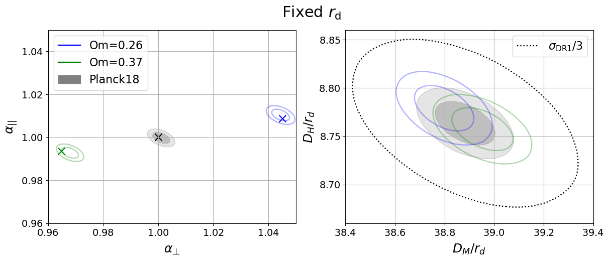
Figure 18: (left) Scale parameters obtained from measurements with the three fiducial cosmologies with fixed $r_{\rm d}$ and different $\Omega_{m}$ and $h$ values. We also include crosses to mark the expected positions of the scale parameters, based on the ratio of their template BAO to that of the template used to create the mocks (Planck 2015). (right) Measured BAO distances obtained by multiplying the scale parameters with the template BAO position. This shows we are able to recover the true BAO position independent of the cosmology used to compute comoving coordinates.

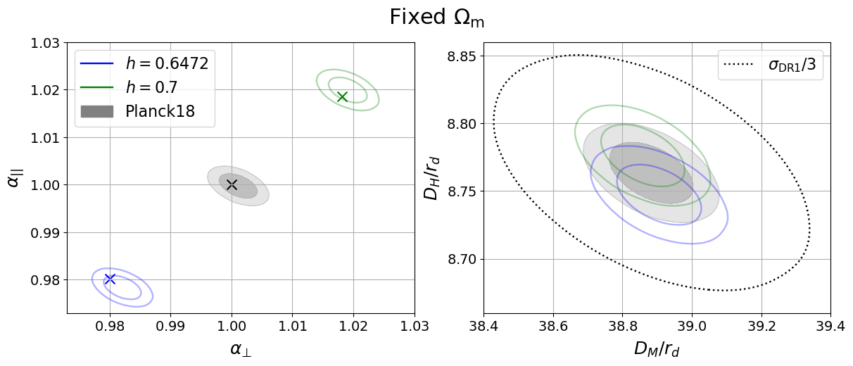
Figure 19: Similar to Figure 18, but using three fiducial cosmologies with fixed coordinate transformation (i.e. $\Omega_{\rm m}$), and different $r_{d}$ values. This shows that we are able to recover the true BAO position independent of the cosmology used to create the template.

In the right panel of Figures 18 and 19, we show the recovered BAO distances, obtained by multiplying the measured scale parameter (contour in the left-hand plot) by the template BAO position (table 3). Also highlighted on this plot is the DESI DR1 $\sigma/3$, the limit given to variations around the baseline analysis in DESI2024-Ly$\alpha$. These figures show that we are able to recover the correct $D_{\rm H}/r_{\rm d}$ and $D_{\rm M}/r_{\rm d}$ values to within $1/10$ of the DESI DR1 uncertainty. This also corresponds to the level at which we can trust the current generation of mocks given the results in Figure 7. Therefore, we conclude that at the level of DESI DR1, we do not detect a significant systematic offset due to the input fiducial cosmology.

In Table 4, we also show the measured BAO amplitude $A_{\rm BAO}$, which we treat as a free parameter for this test. This parameter modifies Equation 3.24 such that:

$$\xi(r_{||},r_{\bot})=\hat{\xi}_{\mathrm{s}}(r_{||},r_{\bot})+A_{\rm BAO}\hat{\xi}_{\mathrm{p}}(\alpha_{||}r_{||},\alpha_{\bot}r_{\bot}),$$ (B.1)

and therefore it fits for differences between the template and the measured amplitude of the BAO peak. Note that this is fixed to $A_{\rm BAO}=1$ for the rest of this work, and also in DESI2024-Ly$\alpha$. As shown in Table 4, we find that the recovered value for this parameter changes depending on the fiducial cosmology. For the cases where we vary $\Omega_{m}h^{2}$, the ratio $\Omega_{c}h^{2}$/$\Omega_{b}h^{2}$ also varies, and therefore the BAO amplitude as well. For the cases where we change $\Omega_{m}$, it is not as straightforward. It could be explained by the fact that f$\sigma_{8}$ changes, which affects the value of $b_{Ly\alpha}$ and leads to different BAO amplitudes, as $A_{\rm BAO}$ is correlated with $b_{Ly\alpha}$. However, as we do not use this parameter to constrain cosmology, we defer an in-depth study of its reliance on the fiducial cosmology to future work.

Appendix C Author Affiliations

¹Center for Cosmology and AstroParticle Physics, The Ohio State University, 191 West Woodruff Avenue, Columbus, OH 43210, USA

²Departamento de Física, Universidad de Guanajuato - DCI, C.P. 37150, Leon, Guanajuato, México

³Institut de Física d’Altes Energies (IFAE), The Barcelona Institute of Science and Technology, Campus UAB, 08193 Bellaterra Barcelona, Spain

⁴Department of Astronomy, The Ohio State University, 4055 McPherson Laboratory, 140 W 18th Avenue, Columbus, OH 43210, USA

⁵Lawrence Berkeley National Laboratory, 1 Cyclotron Road, Berkeley, CA 94720, USA

⁶Consejo Nacional de Ciencia y Tecnología, Av. Insurgentes Sur 1582. Colonia Crédito Constructor, Del. Benito Juárez C.P. 03940, México D.F. México

⁷IRFU, CEA, Université Paris-Saclay, F-91191 Gif-sur-Yvette, France

⁸Physics Dept., Boston University, 590 Commonwealth Avenue, Boston, MA 02215, USA

⁹Department of Physics and Astronomy, University of California, Irvine, 92697, USA

¹⁰Department of Physics & Astronomy, University College London, Gower Street, London, WC1E 6BT, UK

¹¹Instituto de Física, Universidad Nacional Autónoma de México, Cd. de México C.P. 04510, México

¹²Kavli Institute for Particle Astrophysics and Cosmology, Stanford University, Menlo Park, CA 94305, USA

¹³SLAC National Accelerator Laboratory, Menlo Park, CA 94305, USA

¹⁴University of California, Berkeley, 110 Sproul Hall #5800 Berkeley, CA 94720, USA

¹⁵Departamento de Física, Universidad de los Andes, Cra. 1 No. 18A-10, Edificio Ip, CP 111711, Bogotá, Colombia

¹⁶Observatorio Astronómico, Universidad de los Andes, Cra. 1 No. 18A-10, Edificio H, CP 111711 Bogotá, Colombia

¹⁷Institut d’Estudis Espacials de Catalunya (IEEC), 08034 Barcelona, Spain

¹⁸Institute of Cosmology and Gravitation, University of Portsmouth, Dennis Sciama Building, Portsmouth, PO1 3FX, UK

¹⁹Institute of Space Sciences, ICE-CSIC, Campus UAB, Carrer de Can Magrans s/n, 08913 Bellaterra, Barcelona, Spain

²⁰Fermi National Accelerator Laboratory, PO Box 500, Batavia, IL 60510, USA

²¹Department of Physics, The Ohio State University, 191 West Woodruff Avenue, Columbus, OH 43210, USA

²²School of Mathematics and Physics, University of Queensland, 4072, Australia

²³Sorbonne Université, CNRS/IN2P3, Laboratoire de Physique Nucléaire et de Hautes Energies (LPNHE), FR-75005 Paris, France

²⁴Departament de Física, Serra Húnter, Universitat Autònoma de Barcelona, 08193 Bellaterra (Barcelona), Spain

²⁵NSF NOIRLab, 950 N. Cherry Ave., Tucson, AZ 85719, USA

²⁶Institució Catalana de Recerca i Estudis Avançats, Passeig de Lluís Companys, 23, 08010 Barcelona, Spain

²⁷Department of Physics and Astronomy, Siena College, 515 Loudon Road, Loudonville, NY 12211, USA

²⁸Department of Physics & Astronomy, University of Wyoming, 1000 E. University, Dept. 3905, Laramie, WY 82071, USA

²⁹Instituto Avanzado de Cosmología A. C., San Marcos 11 - Atenas 202. Magdalena Contreras, 10720. Ciudad de México, México

³⁰Department of Physics and Astronomy, University of Waterloo, 200 University Ave W, Waterloo, ON N2L 3G1, Canada

³¹Perimeter Institute for Theoretical Physics, 31 Caroline St. North, Waterloo, ON N2L 2Y5, Canada

³²Waterloo Centre for Astrophysics, University of Waterloo, 200 University Ave W, Waterloo, ON N2L 3G1, Canada

³³Space Sciences Laboratory, University of California, Berkeley, 7 Gauss Way, Berkeley, CA 94720, USA

³⁴Instituto de Astrofísica de Andalucía (CSIC), Glorieta de la Astronomía, s/n, E-18008 Granada, Spain

³⁵Departament de Física, EEBE, Universitat Politècnica de Catalunya, c/Eduard Maristany 10, 08930 Barcelona, Spain

³⁶Aix Marseille Univ, CNRS/IN2P3, CPPM, Marseille, France

³⁷Université Clermont-Auvergne, CNRS, LPCA, 63000 Clermont-Ferrand, France

³⁸Department of Physics, Kansas State University, 116 Cardwell Hall, Manhattan, KS 66506, USA

³⁹Department of Physics and Astronomy, Sejong University, Seoul, 143-747, Korea

⁴⁰CIEMAT, Avenida Complutense 40, E-28040 Madrid, Spain

⁴¹Department of Physics, University of Michigan, Ann Arbor, MI 48109, USA

⁴²University of Michigan, Ann Arbor, MI 48109, USA

⁴³Department of Physics & Astronomy, Ohio University, Athens, OH 45701, USA

⁴⁴Excellence Cluster ORIGINS, Boltzmannstrasse 2, D-85748 Garching, Germany

⁴⁵University Observatory, Faculty of Physics, Ludwig-Maximilians-Universität, Scheinerstr. 1, 81677 München, Germany

⁴⁶National Astronomical Observatories, Chinese Academy of Sciences, A20 Datun Rd., Chaoyang District, Beijing, 100012, P.R. China

References

- [1] DESI Collaboration, DESI 2024 IV: Baryon Acoustic Oscillations from the Lyman Alpha Forest, in preparation (2024) .
- [2] D.J. Eisenstein, I. Zehavi, D.W. Hogg, R. Scoccimarro, M.R. Blanton, R.C. Nichol et al., Detection of the Baryon Acoustic Peak in the Large-Scale Correlation Function of SDSS Luminous Red Galaxies, ApJ 633 (2005) 560 [astro-ph/0501171].
- [3] S. Cole, W.J. Percival, J.A. Peacock, P. Norberg, C.M. Baugh, C.S. Frenk et al., The 2dF Galaxy Redshift Survey: power-spectrum analysis of the final data set and cosmological implications, Mon. Not. Roy. Astron. Soc. 362 (2005) 505 [astro-ph/0501174].
- [4] F. Beutler, C. Blake, M. Colless, D.H. Jones, L. Staveley-Smith, L. Campbell et al., The 6dF Galaxy Survey: baryon acoustic oscillations and the local Hubble constant, Mon. Not. Roy. Astron. Soc. 416 (2011) 3017 [1106.3366].
- [5] A.J. Ross, L. Samushia, C. Howlett, W.J. Percival, A. Burden and M. Manera, The clustering of the SDSS DR7 main Galaxy sample - I. A 4 per cent distance measure at z = 0.15, Mon. Not. Roy. Astron. Soc. 449 (2015) 835 [1409.3242].
- [6] S. Alam, M. Ata, S. Bailey, F. Beutler, D. Bizyaev, J.A. Blazek et al., The clustering of galaxies in the completed SDSS-III Baryon Oscillation Spectroscopic Survey: cosmological analysis of the DR12 galaxy sample, Mon. Not. Roy. Astron. Soc. 470 (2017) 2617 [1607.03155].
- [7] T.M.C. Abbott, F.B. Abdalla, A. Alarcon, S. Allam, F. Andrade-Oliveira, J. Annis et al., Dark Energy Survey Year 1 Results: Measurement of the Baryon Acoustic Oscillation scale in the distribution of galaxies to redshift 1, Mon. Not. Roy. Astron. Soc. 483 (2019) 4866 [1712.06209].
- [8] S. Alam, M. Aubert, S. Avila, C. Balland, J.E. Bautista, M.A. Bershady et al., Completed SDSS-IV extended Baryon Oscillation Spectroscopic Survey: Cosmological implications from two decades of spectroscopic surveys at the Apache Point Observatory, Phys. Rev. D 103 (2021) 083533 [2007.08991].
- [9] T.M.C. Abbott, M. Aguena, S. Allam, A. Amon, F. Andrade-Oliveira, J. Asorey et al., Dark Energy Survey Year 3 results: A 2.7% measurement of baryon acoustic oscillation distance scale at redshift 0.835, Phys. Rev. D 105 (2022) 043512 [2107.04646].
- [10] DES Collaboration, T.M.C. Abbott, M. Adamow, M. Aguena, S. Allam, O. Alves et al., Dark Energy Survey: A 2.1% measurement of the angular Baryonic Acoustic Oscillation scale at redshift =0.85 from the final dataset, arXiv e-prints (2024) arXiv:2402.10696 [2402.10696].
- [11] DESI Collaboration, A. Aghamousa, J. Aguilar, S. Ahlen, S. Alam, L.E. Allen et al., The DESI Experiment Part I: Science,Targeting, and Survey Design, arXiv e-prints (2016) arXiv:1611.00036 [1611.00036].
- [12] DESI Collaboration, A. Aghamousa, J. Aguilar, S. Ahlen, S. Alam, L.E. Allen et al., The DESI Experiment Part II: Instrument Design, arXiv e-prints (2016) arXiv:1611.00037 [1611.00037].
- [13] DESI Collaboration, B. Abareshi, J. Aguilar, S. Ahlen, S. Alam, D.M. Alexander et al., Overview of the Instrumentation for the Dark Energy Spectroscopic Instrument, AJ 164 (2022) 207 [2205.10939].
- [14] DESI Collaboration, A.G. Adame, J. Aguilar, S. Ahlen, S. Alam, G. Aldering et al., Validation of the Scientific Program for the Dark Energy Spectroscopic Instrument, AJ 167 (2024) 62 [2306.06307].
- [15] DESI Collaboration, A.G. Adame, J. Aguilar, S. Ahlen, S. Alam, G. Aldering et al., The Early Data Release of the Dark Energy Spectroscopic Instrument, arXiv e-prints (2023) arXiv:2306.06308 [2306.06308].
- [16] DESI Collaboration, DESI 2024 I: Data Release 1 of the Dark Energy Spectroscopic Instrument, in preparation (2024) .
- [17] DESI Collaboration, DESI 2024 II: Sample definitions, characteristics and two-point clustering statistics, in preparation (2024) .
- [18] DESI Collaboration, DESI 2024 III: Baryon Acoustic Oscillations from Galaxies and Quasars, in preparation (2024) .
- [19] DESI Collaboration, DESI 2024 VI: Cosmological Constraints from the Measurements of Baryon Acoustic Oscillations, in preparation (2024) .
- [20] N.G. Busca, T. Delubac, J. Rich, S. Bailey, A. Font-Ribera, D. Kirkby et al., Baryon acoustic oscillations in the Ly forest of BOSS quasars, Astron. Astrophys. 552 (2013) A96 [1211.2616].
- [21] A. Slosar, V. Iršič, D. Kirkby, S. Bailey, N.G. Busca, T. Delubac et al., Measurement of baryon acoustic oscillations in the Lyman- forest fluctuations in BOSS data release 9, JCAP 2013 (2013) 026 [1301.3459].
- [22] D. Kirkby, D. Margala, A. Slosar, S. Bailey, N.G. Busca, T. Delubac et al., Fitting methods for baryon acoustic oscillations in the Lyman- forest fluctuations in BOSS data release 9, JCAP 2013 (2013) 024 [1301.3456].
- [23] K.S. Dawson, D.J. Schlegel, C.P. Ahn, S.F. Anderson, É. Aubourg, S. Bailey et al., The Baryon Oscillation Spectroscopic Survey of SDSS-III, AJ 145 (2013) 10 [1208.0022].
- [24] A. Font-Ribera, D. Kirkby, N. Busca, J. Miralda-Escudé, N.P. Ross, A. Slosar et al., Quasar-Lyman forest cross-correlation from BOSS DR11: Baryon Acoustic Oscillations, JCAP 5 (2014) 27 [1311.1767].
- [25] K.S. Dawson, J.-P. Kneib, W.J. Percival, S. Alam, F.D. Albareti, S.F. Anderson et al., The SDSS-IV Extended Baryon Oscillation Spectroscopic Survey: Overview and Early Data, AJ 151 (2016) 44 [1508.04473].
- [26] T. Delubac, J.E. Bautista, N.G. Busca, J. Rich, D. Kirkby, S. Bailey et al., Baryon acoustic oscillations in the Ly forest of BOSS DR11 quasars, Astron. Astrophys. 574 (2015) A59 [1404.1801].
- [27] J.E. Bautista, N.G. Busca, J. Guy, J. Rich, M. Blomqvist, H. du Mas des Bourboux et al., Measurement of baryon acoustic oscillation correlations at z = 2.3 with SDSS DR12 Ly-Forests, Astron. Astrophys. 603 (2017) A12 [1702.00176].
- [28] H. du Mas des Bourboux, J.-M. Le Goff, M. Blomqvist, N.G. Busca, J. Guy, J. Rich et al., Baryon acoustic oscillations from the complete SDSS-III Ly-quasar cross-correlation function at z = 2.4, Astron. Astrophys. 608 (2017) A130 [1708.02225].
- [29] V. de Sainte Agathe, C. Balland, H. du Mas des Bourboux, N.G. Busca, M. Blomqvist, J. Guy et al., Baryon acoustic oscillations at z = 2.34 from the correlations of Ly absorption in eBOSS DR14, Astron. Astrophys. 629 (2019) A85 [1904.03400].
- [30] M. Blomqvist, H. du Mas des Bourboux, N.G. Busca, V. de Sainte Agathe, J. Rich, C. Balland et al., Baryon acoustic oscillations from the cross-correlation of Ly absorption and quasars in eBOSS DR14, Astron. Astrophys. 629 (2019) A86 [1904.03430].
- [31] H. du Mas des Bourboux, J. Rich, A. Font-Ribera, V. de Sainte Agathe, J. Farr, T. Etourneau et al., The Completed SDSS-IV Extended Baryon Oscillation Spectroscopic Survey: Baryon Acoustic Oscillations with Ly Forests, ApJ 901 (2020) 153 [2007.08995].
- [32] H. Bi and A.F. Davidsen, Evolution of Structure in the Intergalactic Medium and the Nature of the Ly Forest, ApJ 479 (1997) 523 [astro-ph/9611062].
- [33] R.A.C. Croft, D.H. Weinberg, N. Katz and L. Hernquist, Recovery of the Power Spectrum of Mass Fluctuations from Observations of the Ly Forest, ApJ 495 (1998) 44 [astro-ph/9708018].
- [34] C. Ramírez-Pérez, J. Sanchez, D. Alonso and A. Font-Ribera, CoLoRe: fast cosmological realisations over large volumes with multiple tracers, JCAP 2022 (2022) 002 [2111.05069].
- [35] J. Farr, A. Font-Ribera, H. du Mas des Bourboux, A. Muñoz-Gutiérrez, F.J. Sánchez, A. Pontzen et al., LyaCoLoRe: synthetic datasets for current and future Lyman- forest BAO surveys, JCAP 2020 (2020) 068 [1912.02763].
- [36] T. Etourneau, J.-M. Le Goff, J. Rich, T. Tan, A. Cuceu, S. Ahlen et al., Mock data sets for the Eboss and DESI Lyman- forest surveys, arXiv e-prints (2023) arXiv:2310.18996 [2310.18996].
- [37] H.K. Herrera-Alcantar, A. Muñoz-Gutiérrez, T. Tan, A.X. González-Morales, A. Font-Ribera, J. Guy et al., Synthetic spectra for Lyman- forest analysis in the Dark Energy Spectroscopic Instrument, arXiv e-prints (2023) arXiv:2401.00303 [2401.00303].
- [38] P. Laurent, S. Eftekharzadeh, J.-M. Le Goff, A. Myers, E. Burtin, M. White et al., Clustering of quasars in SDSS-IV eBOSS: study of potential systematics and bias determination, JCAP 2017 (2017) 017 [1705.04718].
- [39] A. Cuceu, A. Font-Ribera, P. Martini, B. Joachimi, S. Nadathur, J. Rich et al., The Alcock-Paczyński effect from Lyman- forest correlations: analysis validation with synthetic data, Mon. Not. Roy. Astron. Soc. 523 (2023) 3773 [2209.12931].
- [40] Planck Collaboration, P.A.R. Ade, N. Aghanim, M. Arnaud, M. Ashdown, J. Aumont et al., Planck 2015 results. XIII. Cosmological parameters, Astron. Astrophys. 594 (2016) A13 [1502.01589].
- [41] Planck Collaboration, N. Aghanim, Y. Akrami, M. Ashdown, J. Aumont, C. Baccigalupi et al., Planck 2018 results. VI. Cosmological parameters, Astron. Astrophys. 641 (2020) A6 [1807.06209].
- [42] K.M. Górski, E. Hivon, A.J. Banday, B.D. Wandelt, F.K. Hansen, M. Reinecke et al., HEALPix: A Framework for High-Resolution Discretization and Fast Analysis of Data Distributed on the Sphere, ApJ 622 (2005) 759 [astro-ph/0409513].
- [43] E.F. Schlafly, D. Kirkby, D.J. Schlegel, A.D. Myers, A. Raichoor, K. Dawson et al., Survey Operations for the Dark Energy Spectroscopic Instrument, AJ 166 (2023) 259 [2306.06309].
- [44] J. Guy, S. Bailey, A. Kremin, S. Alam, D.M. Alexander, C. Allende Prieto et al., The Spectroscopic Data Processing Pipeline for the Dark Energy Spectroscopic Instrument, AJ 165 (2023) 144 [2209.14482].
- [45] S. Youles, J.E. Bautista, A. Font-Ribera, D. Bacon, J. Rich, D. Brooks et al., The effect of quasar redshift errors on Lyman- forest correlation functions, Mon. Not. Roy. Astron. Soc. 516 (2022) 421 [2205.06648].
- [46] S. Filbert, P. Martini, K. Seebaluck, L. Ennesser, D.M. Alexander, A. Bault et al., Broad Absorption Line Quasars in the Dark Energy Spectroscopic Instrument Early Data Release, arXiv e-prints (2023) arXiv:2309.03434 [2309.03434].
- [47] D. Kirkby, S. Bailey, J. Guy and B.A. Weaver, Quick simulations of fiber spectrograph response v0.5, Sept., 2016. 10.5281/zenodo.154130.
- [48] C. Ramírez-Pérez, I. Pérez-Ràfols, A. Font-Ribera, M.A. Karim, E. Armengaud, J. Bautista et al., The Lyman- forest catalogue from the Dark Energy Spectroscopic Instrument Early Data Release, Mon. Not. Roy. Astron. Soc. 528 (2024) 6666 [2306.06312].
- [49] B. Wang, J. Zou, Z. Cai, J.X. Prochaska, Z. Sun, J. Ding et al., Deep Learning of Dark Energy Spectroscopic Instrument Mock Spectra to Find Damped Ly Systems, ApJS 259 (2022) 28.
- [50] L. Ennesser, P. Martini, A. Font-Ribera and I. Pérez-Ràfols, The impact and mitigation of broad-absorption-line quasars in Lyman forest correlations, Mon. Not. Roy. Astron. Soc. 511 (2022) 3514 [2111.09439].
- [51] P. Noterdaeme, P. Petitjean, W.C. Carithers, I. Pâris, A. Font-Ribera, S. Bailey et al., Column density distribution and cosmological mass density of neutral gas: Sloan Digital Sky Survey-III Data Release 9, Astron. Astrophys. 547 (2012) L1 [1210.1213].
- [52] I. Pérez-Ràfols, A. Font-Ribera, J. Miralda-Escudé, M. Blomqvist, S. Bird, N. Busca et al., The SDSS-DR12 large-scale cross-correlation of damped Lyman alpha systems with the Lyman alpha forest, Mon. Not. Roy. Astron. Soc. 473 (2018) 3019 [1709.00889].
- [53] P. McDonald, U. Seljak, S. Burles, D.J. Schlegel, D.H. Weinberg, R. Cen et al., The Ly Forest Power Spectrum from the Sloan Digital Sky Survey, ApJS 163 (2006) 80 [astro-ph/0405013].
- [54] C. Gordon, A. Cuceu, J. Chaves-Montero, A. Font-Ribera, A.X. González-Morales, J. Aguilar et al., 3D correlations in the Lyman- forest from early DESI data, JCAP 2023 (2023) 045 [2308.10950].
- [55] H. du Mas des Bourboux, K.S. Dawson, N.G. Busca, M. Blomqvist, V. de Sainte Agathe, C. Balland et al., The Extended Baryon Oscillation Spectroscopic Survey: Measuring the Cross-correlation between the Mg II Flux Transmission Field and Quasars and Galaxies at z = 0.59, ApJ 878 (2019) 47 [1901.01950].
- [56] N. Kaiser, Clustering in real space and in redshift space, Mon. Not. Roy. Astron. Soc. 227 (1987) 1.
- [57] A. Lewis, A. Challinor and A. Lasenby, Efficient computation of CMB anisotropies in closed FRW models, ApJ 538 (2000) 473 [astro-ph/9911177].
- [58] A. Font-Ribera and J. Miralda-Escudé, The effect of high column density systems on the measurement of the Lyman- forest correlation function, JCAP 2012 (2012) 028 [1205.2018].
- [59] M. McQuinn and M. White, On estimating Ly forest correlations between multiple sightlines, Mon. Not. Roy. Astron. Soc. 415 (2011) 2257 [1102.1752].
- [60] P. Noterdaeme, P. Petitjean, C. Ledoux and R. Srianand, Evolution of the cosmological mass density of neutral gas from Sloan Digital Sky Survey II - Data Release 7, Astron. Astrophys. 505 (2009) 1087 [0908.1574].
- [61] J.X. Prochaska, J.M. O’Meara and G. Worseck, A Definitive Survey for Lyman Limit Systems at z ~3.5 with the Sloan Digital Sky Survey, ApJ 718 (2010) 392 [0912.0292].
- [62] T. Zafar, C. Péroux, A. Popping, B. Milliard, J.M. Deharveng and S. Frank, The ESO UVES advanced data products quasar sample. II. Cosmological evolution of the neutral gas mass density, Astron. Astrophys. 556 (2013) A141 [1307.0602].
- [63] A. Cuceu, A. Font-Ribera and B. Joachimi, Bayesian methods for fitting Baryon Acoustic Oscillations in the Lyman- forest, JCAP 2020 (2020) 035 [2004.02761].
- [64] W.J. Percival and M. White, Testing cosmological structure formation using redshift-space distortions, Mon. Not. Roy. Astron. Soc. 393 (2009) 297 [0808.0003].
- [65] A. Arinyo-i-Prats, J. Miralda-Escudé, M. Viel and R. Cen, The non-linear power spectrum of the Lyman alpha forest, JCAP 2015 (2015) 017 [1506.04519].
- [66] A.J.S. Hamilton, Uncorrelated modes of the non-linear power spectrum, Mon. Not. Roy. Astron. Soc. 312 (2000) 257 [astro-ph/9905191].
- [67] H. Dembinski and P.O. et al., scikit-hep/iminuit, .
- [68] F. James and M. Roos, Minuit: A System for Function Minimization and Analysis of the Parameter Errors and Correlations, Comput. Phys. Commun. 10 (1975) 343.
- [69] W.J. Handley, M.P. Hobson and A.N. Lasenby, polychord: nested sampling for cosmology., Mon. Not. Roy. Astron. Soc. 450 (2015) L61 [1502.01856].
- [70] W.J. Handley, M.P. Hobson and A.N. Lasenby, POLYCHORD: next-generation nested sampling, Mon. Not. Roy. Astron. Soc. 453 (2015) 4384 [1506.00171].
- [71] A. Font-Ribera, E. Arnau, J. Miralda-Escudé, E. Rollinde, J. Brinkmann, J.R. Brownstein et al., The large-scale quasar-Lyman forest cross-correlation from BOSS, JCAP 2013 (2013) 018 [1303.1937].
- [72] A. Bault, D. Kirkby, J. Guy, A. Brodzeller, J. Aguilar, S. Ahlen et al., Impact of Systematic Redshift Errors on the Cross-correlation of the Lyman- Forest with Quasars at Small Scales Using DESI Early Data, arXiv e-prints (2024) arXiv:2402.18009 [2402.18009].
- [73] A. Cuceu, A. Font-Ribera, B. Joachimi and S. Nadathur, Cosmology beyond BAO from the 3D distribution of the Lyman- forest, Mon. Not. Roy. Astron. Soc. 506 (2021) 5439 [2103.14075].
- [74] J.J. Givans, A. Font-Ribera, A. Slosar, L. Seeyave, C. Pedersen, K.K. Rogers et al., Non-linearities in the Lyman- forest and in its cross-correlation with dark matter halos, JCAP 2022 (2022) 070 [2205.00962].
- [75] B. Hadzhiyska et al., Planting a Lyman alpha forest on AbacusSummit, Mon. Not. Roy. Astron. Soc. 524 (2023) 1008 [2305.08899].
- [76] D.J. Eisenstein, H.-J. Seo and M. White, On the Robustness of the Acoustic Scale in the Low-Redshift Clustering of Matter, ApJ 664 (2007) 660 [astro-ph/0604361].
- [77] F. Sinigaglia, F.-S. Kitaura, A. Balaguera-Antolínez, I. Shimizu, K. Nagamine, M. Sánchez-Benavente et al., Mapping the Three-dimensional Ly Forest Large-scale Structure in Real and Redshift Space*, Astrophys. J. 927 (2022) 230 [2107.07917].
- [78] F. Sinigaglia, F.-S. Kitaura, K. Nagamine, Y. Oku and A. Balaguera-Antolínez, Field-level Lyman-alpha forest modelling in redshift space via augmented non-local Fluctuating Gunn-Peterson Approximation, 2305.10428.
- [79] I. Pérez-Ràfols, M.M. Pieri, M. Blomqvist, S. Morrison, D. Som and A. Cuceu, The cross-correlation of galaxies in absorption with the Lyman forest, Mon. Not. Roy. Astron. Soc. 524 (2023) 1464 [2210.02973].
- [80] J. Guy, S. Bailey, A. Kremin, S. Alam, D.M. Alexander, C. Allende Prieto et al., The Spectroscopic Data Processing Pipeline for the Dark Energy Spectroscopic Instrument, AJ 165 (2023) 144 [2209.14482].
- [81] J. Guy, S. Gontcho A Gontcho et al., Characterization of contaminants in the Lyman-alpha forest auto-correlation with DESI, in preparation (2024) .
- [82] A. Pontzen, Scale-dependent bias in the baryonic-acoustic-oscillation-scale intergalactic neutral hydrogen, Phys. Rev. D 89 (2014) 083010 [1402.0506].
- [83] S. Gontcho A Gontcho, J. Miralda-Escudé and N.G. Busca, On the effect of the ionizing background on the Ly forest autocorrelation function, Mon. Not. Roy. Astron. Soc. 442 (2014) 187 [1404.7425].
- [84] C.R. Harris, K.J. Millman, S.J. van der Walt, R. Gommers, P. Virtanen, D. Cournapeau et al., Array programming with NumPy, Nature 585 (2020) 357.
- [85] P. Virtanen, R. Gommers, T.E. Oliphant, M. Haberland, T. Reddy, D. Cournapeau et al., SciPy 1.0: fundamental algorithms for scientific computing in Python, Nature Methods 17 (2020) 261 [1907.10121].
- [86] Astropy Collaboration, T.P. Robitaille, E.J. Tollerud, P. Greenfield, M. Droettboom, E. Bray et al., Astropy: A community Python package for astronomy, Astron. Astrophys. 558 (2013) A33 [1307.6212].
- [87] Astropy Collaboration, A.M. Price-Whelan, B.M. Sipőcz, H.M. Günther, P.L. Lim, S.M. Crawford et al., The Astropy Project: Building an Open-science Project and Status of the v2.0 Core Package, AJ 156 (2018) 123 [1801.02634].
- [88] Astropy Collaboration, A.M. Price-Whelan, P.L. Lim, N. Earl, N. Starkman, L. Bradley et al., The Astropy Project: Sustaining and Growing a Community-oriented Open-source Project and the Latest Major Release (v5.0) of the Core Package, ApJ 935 (2022) 167 [2206.14220].
- [89] L. Dalcin and Y.-L.L. Fang, mpi4py: Status update after 12 years of development, Computing in Science & Engineering 23 (2021) 47.
- [90] A. Zonca, L. Singer, D. Lenz, M. Reinecke, C. Rosset, E. Hivon et al., healpy: equal area pixelization and spherical harmonics transforms for data on the sphere in python, Journal of Open Source Software 4 (2019) 1298.
- [91] J.D. Hunter, Matplotlib: A 2d graphics environment, Computing in Science & Engineering 9 (2007) 90.
- [92] A. Lewis, GetDist: a Python package for analysing Monte Carlo samples, arXiv e-prints (2019) arXiv:1910.13970 [1910.13970].
- [93] S.K. Lam, A. Pitrou and S. Seibert, Numba: A LLVM-based Python JIT Compiler, in Proc. Second Workshop on the LLVM Compiler Infrastructure in HPC, pp. 1–6, Nov., 2015, DOI.