Characterization of contaminants in the Lyman-alpha forest auto-correlation with DESI

Abstract

Baryon Acoustic Oscillations can be measured with sub-percent precision above redshift two with the Lyman-$\alpha$ (Ly$\alpha$) forest auto-correlation and its cross-correlation with quasar positions. This is one of the key goals of the Dark Energy Spectroscopic Instrument (DESI) which started its main survey in May 2021. We present in this paper a study of the contaminants to the Ly$\alpha$ forest which are mainly caused by correlated signals introduced by the spectroscopic data processing pipeline as well as astrophysical contaminants due to foreground absorption in the intergalactic medium. Notably, an excess signal caused by the sky background subtraction noise is present in the Ly$\alpha$ auto-correlation in the first line-of-sight separation bin. We use synthetic data to isolate this contribution, we also characterize the effect of spectro-photometric calibration noise, and propose a simple model to account for both effects in the analysis of the Ly$\alpha$ forest. We then measure the auto-correlation of the quasar flux transmission fraction of low redshift quasars, where there is no Ly$\alpha$ forest absorption but only its contaminants. We demonstrate that we can interpret the data with a two-component model: data processing noise and triply ionized Silicon and Carbon auto-correlations. This result can be used to improve the modeling of the Ly$\alpha$ auto-correlation function measured with DESI.

1 Introduction

Precisely measuring the expansion history of the universe allows one to discriminate between different theories of dark energy, the putative cause of the presently observed accelerated expansion of the universe [1, 2, 3]. One method to access the redshift-dependent expansion rate, and the probe of interest of this paper, uses baryon acoustic oscillations (BAO) [4]. In this work, we investigate pipeline-induced and astrophysical sources of systematic uncertainties in this measurement at high redshift.

The BAO-induced feature in cosmological correlation functions is used as a standard ruler whose characteristic scale has been measured with ever greater precision in the distribution of galaxies from large scale redshift surveys: the Sloan Digital Sky Survey (SDSS) I and II [5, 6, 7], the 2-degree Field Galaxy Redshift Survey (2dFGRS) [8, 9], WiggleZ [10], the 6-degree Field Galaxy Survey (6dFGS) [11], the Baryon Oscillation Spectroscopic Survey (BOSS) part of SDSS III [12] and finally the extended BOSS survey (eBOSS) with [13, 14] up to a redshift of $z<2.0$.

Aside from galaxies, a powerful tracer of the large scale structure of the universe is the intergalactic medium. Specifically, leveraging the series of absorption features of neutral hydrogen gas in quasars spectra, called the Lyman-$\alpha$ forest, has provided measurements of the BAO scale at redshift $z\,\sim\,2.3$ : first with BOSS [15, 16, 17, 18, 19, 20, 21] and then with eBOSS [22, 23, 24]. Owing to the fact that ground-based large scale cosmological surveys observe in the optical range, the Lyman-$\alpha$ forest data collected allow one to probe the distribution of neutral hydrogen gas at $z\,>\,2.1$. This redshift range is complementary to that of the galaxies observed by the same surveys. At its best, the Lyman-$\alpha$ forest has provided an isotropic BAO measurement with a precision of 1.3% [24].

The Dark Energy Spectroscopic Instrument (DESI) is the newest generation of fully operational ground-based multi-object spectroscopic instruments. Seeing first light on October 22, 2019 and starting the first of its five-year survey on May 14, 2021, DESI is expected to deliver percent-level BAO measurements from its $z\,>\,2.1$ quasar redshift sample and their Ly$\alpha$  forests. This expected improvement in the precision of the Ly$\alpha$  BAO measurement compared to previous surveys is due in part to the fact that DESI will observe quadruple as much $z\,>\,2.1$ quasars as that available in the final eBOSS sample. Another key point to delivering a strong cosmological measurement is a solid understanding of the systematics introduced by the DESI instrument and its pipeline, as well as the astrophysical systematics at our level of sensitivity.

Studies of the sort have been conducted and mentioned in [20] and [24] to understand the systematics introduced by BOSS/eBOSS instruments and pipelines. The dominant effect was found to be a small excess correlation in the Ly$\alpha$ auto-correlation function for pixel pairs of the same wavelength. This effect results from a common noise introduced in neighboring fibers when subtracting the sky background.

We revisit those studies in the context of DESI. We first assess the spurious correlated signal introduced in the Ly$\alpha$  auto-correlation by the spectroscopic pipeline (this does not affect the cross-correlation with quasars). We demonstrate our understanding of the source of those pipeline-induced correlations by modeling the sky background subtraction noise and the spectrophotometric calibration noise so they can be accounted for in the DESI analysis of the Ly$\alpha$  autocorrelation [25, 26]. Then we characterize the signal from astronomical contaminants due to foreground absorption. To do so, we measure the auto-correlation of the quasar flux transmission fraction of low redshift quasars, where there is no Ly$\alpha$  forest absorption but only its contaminants; i.e. other chemical species, or metals, such as triply ionized silicon (SiIV), triply ionized carbon (CIV) and ionized magnesium (MgII) [27]. In the same way that we define the Ly$\alpha$ forest, the series of absorption features at wavelengths smaller than the SiIV (resp. CIV, resp. MgII) emission peak/doublet is called the SiIV forest (resp. CIV forest, resp. MgII forest).

The paper is organized as follows. Section 2 presents the details of the DESI Survey and the first year dataset used in this study. Section 3 gives an overview of the Lyman-$\alpha$ forest analysis. The data processing noise correlation is then characterized and modeled in section 4. This model is validated when studying the auto-correlation of foreground absorbers in section 5. Section 6 provides a summary of our findings and the implications for the fit of the DESI Ly$\alpha$ auto-correlation function.

2 The DESI Survey

The Dark Energy Spectroscopic Instrument (DESI) project is measuring the redshifts of more than 40 million galaxies and quasars over 14,000 sq. deg. of the northern sky, effectively building the largest three dimensional map of the observable universe. Its goal is to measure the cosmic expansion history and the growth of large scale structure to great precision in order to gain insight into the nature of dark energy.

The DESI instrument is presented in detail in [28] and references therein; we provide here only a brief overview. DESI is a multi object spectroscopic system installed at the Mayall 4-m telescope at Kitt Peak National Observatory near Tucson in Arizona, USA. It features a prime focus instrument with a specially designed corrector and a focal plane comprised of 5000 robotic fiber positioners [29] connected to ten 3-arm spectrographs. Specifically, the focal plane is divided into 10 petals each containing 500 fibers. Each 500-fibers bundle is connected to one spectrograph. Each spectrograph is made up of a blue channel spanning 3600 Å  to 5930 Å, a red channel spanning 5600 Å  to 7720 Å  and a near infrared channel spanning 7470 Å  to 9800 Å. The spectrographs have a spectral resolution ranging from 2000 to 5000, see [30]. A set of 5000 astronomical objects observed simultaneously by one pointing of the telescope is called a tile.

The DESI spectroscopic pipeline is run immediately after the observations, once they have been uploaded from Kitt Peak down to the National Energy Research Scientific Computing Center, providing fully reduced spectra and redshifts within hours, along with quality diagnostics to validate the data set. The pipeline is also re-run with a uniform set of codes and calibrations for each data release. In practice, this means: processing nightly calibration images (zeros, arcs, and flats), finding wavelength and line-spread-function solutions for each exposure, extracting the one-dimensional spectra from the two-dimensional frames, flat-fielding the spectra, subtracting a sky background model and calibrating fluxes, determining redshifts and classifications for each spectrum, and evaluating the quality of the data. The spectroscopic pipeline is described in more detail in [30]. Refer specifically to Figure 5 for a complete and detailed diagram of the spectroscopic pipeline data flow.

The survey, intended to operate for 5 years, is now well advanced. When the moon is below the horizon, also called dark time (see [31]), the DESI survey observes three categories of astronomical objects of interest to be used as tracers of the matter density field. They are the Luminous Red Galaxies (LRG), the Emission Line Galaxies (ELG) and the quasars – also referred to as Quasi Stellar Objects (QSOs). These tracers are spanning the range $0.4<z<4$, where the upper limit is defined by the scarcity of intrinsically bright high redshift quasars. Only quasars at redshifts $z>2.1$ can be used for the study of Ly$\alpha$ forests because of the UV cutoff of the spectrograph sensitivity and the atmospheric transmission. DESI targeted about 60 quasars per square degree (see [32]). At the end of the 5 year survey, we expect to have short of 1,000,000 Ly$\alpha$  forests. That is $\sim 4$ times more than BOSS and eBOSS. This will result in cosmological constraints from the Ly$\alpha$  forest at the sub-percent level precision [33, 34].

To be able to exploit the information stored in the Ly$\alpha$  forests in the spectra of $z>2.1$ quasars, the signal-to-noise requirements are higher than the fiducial requirements for redshift identification for all the other target classes. As such, quasars that will be used for Ly$\alpha$  analysis need three to four times the amount of DESI fiducial dark time [31].

The state of each potential DESI target, i.e. whether they need extra observations, is tracked through the Merged Target List (MTL, see [35]). Following each successful exposure and quality assurance check, the archived results of the spectroscopic analysis are used to update the MTL, adjusting the priorities of observed targets. Most importantly, newly detected Ly$\alpha$  quasars are the highest priority targets in the main survey (before other galaxy classes) and should therefore be observed whenever possible.

Apart from the signal-to-noise requirements in the Ly$\alpha$  forest region, another key point is to accurately measure the redshift of the observed quasars. To that end, the standard DESI pipeline (i.e. the automated spectroscopic data reduction), described in [30], applies a template-fitting code called Redrock [36] to derive classifications and redshifts for each target. This is combined with line-fitting “afterburner” codes, QuasarNET [37, 38] and a MgII afterburner, that are incorporated at the level of the MTL logic. The MTL takes into account redshifts and redshift warnings from Redrock, as well as quasar classifications and redshifts from QuasarNET when updating the state of a given target.

The redshifts are used to update the MTL, promoting newly detected $z>2.1$ quasars to high priority targets which should be observed whenever possible.

The main survey was started on May 14, 2021. We use in this analysis spectra from the first year of data which will be published as part of the DESI first data release (DR1). The quasar catalog used for this analysis relies on the DESI catalog from [39]. Compared to the DESI Early Data Release [32], this catalog is enriched with new redshifts calculated by using updated quasar templates from [40] and an improved Redrock version. This addresses a bias on redshifts $z>2$ identified through the Ly$\alpha$  quasar cross-correlation [41]. The updated redshift catalog is set for release alongside DR1. Following the definitions from Table 3 in [30], quasars passing a quality threshold are retained, while those with reported pipeline issues are discarded. Utilizing the HEALPix [43] coadded quasar spectra from the DR1 reduction of the main survey dark time program, we identify Damped Lyman-$\alpha$ Systems (DLAs) through two methods: Convolution Neural Network and Gaussian Processes (see [44]). Notably, we refrain from rerunning the DLA finder with the new quasar redshift catalog due to the substantial time investment required. DLAs with neutral hydrogen column densities surpassing $2\times 10^{20}$ cm^-2 are masked based on high-confidence detection and in accordance with the prescriptions from [44]. Additionally, quasars with Broad Absorption Lines (BALs) are identified using the algorithm outlined in [45], and contaminated regions in the spectra are masked following [46] guidelines.

For the analysis presented in this paper, we use the MgII, CIV, SiIV and Ly$\alpha$  forests. Depending on the forest considered, and therefore the corresponding redshift of the background quasar, we have short of half a million spectra at $z>2.1$ and about a million at lower redshifts. The choice has been made to measure the transmitted flux fraction fluctuations in the observed wavelength range 3600 - 5772 Å  [26], falling squarely onto the blue cameras of the DESI spectrographs. We define the following four distinct spectral regions of the quasar rest-frame spectrum: the Ly$\alpha$  forest (1040 – 1205 Å), the CIV forest (1420 – 1520 Å), the SiIV forest (1260 – 1375 Å) and the MgII forest (1920 – 2760 Å).

3 Analysis of the Lyman-$\alpha$ forest

We provide a high level description of how we access cosmological information by looking at absorption features from quasar spectra. More details can be found in [20, 24] for the BOSS and eBOSS analyses and [25, 26] for the more recent analyses of the DESI Early Data.

We use the Ly$\alpha$ transmitted flux fraction $F(\lambda)$ in high redshift quasar spectra as tracer of the matter over density at redshift $z_{\alpha}=\lambda/\lambda_{\alpha}-1$, where $\lambda_{\alpha}=1215.67$ Å is the Lyman-$\alpha$ transition wavelength in the Lyman series. We call $\delta_{q}(\lambda)=F_{q}(\lambda)/\overline{F}(\lambda)-1$ the transmitted flux fraction fluctuation in a quasar spectrum $q$. $\delta_{q}$ is obtained by dividing the observed quasar spectrum $f_{q}$ by an estimate of the unabsorbed quasar spectrum $C_{q}$ times the mean transmission flux fraction $\overline{F}$. $C_{q}$ is often referred to as continuum.

$$\delta_{q}(\lambda)\equiv\frac{f_{q}(\lambda)}{C_{q}\overline{F}(\lambda)}-1$$ (3.1)

The average flux transmission fraction $\overline{F}$ evolves smoothly with redshift following the variation of neutral hydrogen density and hence is a function of the observer frame wavelength $\lambda$. In practice we approximate the product $C_{q}\overline{F}(\lambda)$ by the average absorbed quasar spectrum times a correction to account for the specific amplitude and slope of the spectrum in the Ly$\alpha$ forest: $C_{q}\overline{F}(\lambda)\simeq\overline{CF}(\lambda_{RF})(a_{q}+b_{q}\log\lambda)$, where $\lambda_{RF}$ stands for the quasar rest-frame wavelength. This is computed with an iterative procedure (as described in [25]).

The estimator of the auto-correlation function that takes as input the transmitted flux fraction fluctuation is

$$\xi_{A}=\frac{\sum_{i,j\in A}w_{i}w_{j}\delta_{i}\delta_{j}}{\sum_{i,j\in A}w_{i}w_{j}},$$ (3.2)

where $i$ (resp. $j$) is an index that indicates a measurement on quasars $q_{i}$ (resp. $q_{j}$) at wavelength $\lambda_{i}$ (resp. $\lambda_{j}$) using the weights $w_{i}$ (resp. $w_{j}$) and the forest element $\delta_{i}$ (resp. $\delta_{j}$). The weights are optimized to account for the intrinsic fluctuations introduced by cosmological large scale structures, as well as measurement noise. Pairs (i, j) belonging to the same quasar are excluded to prevent contamination by correlated errors introduced by the estimation of $C_{q}(\lambda)$ for a given spectrum. $A$ denotes the bin in the space of co-moving separation $(r_{\perp},r_{\parallel})$ where $r_{\parallel}$ means distance of separation along the line of sight and $r_{\perp}$ refers to the distance of separation perpendicular to the line of sight. We elect for the bins to be of 4 $h^{-1}$Mpc  in both directions and evaluate the correlation function from 0 to 200 $h^{-1}$Mpc.

One should be aware that the measurement of the normalization and slope of a quasar spectrum in the computation of $\delta_{q}(\lambda)$ introduces correlations among the values of $\delta_{q}$ at different wavelengths in the same spectrum. To a good approximation, the resulting quantity is a linear combination of the original $\delta_{q}$. The linear transformation is actually enforced in the correlation function estimator where values $\hat{\delta}_{q}$ are computed from the $\delta_{q}$ by explicitly subtracting the weighted mean and slope along each line of sight. This linear transformation is called a “projection” in [24] (see their Eq. 5 and 6). It results that the measured correlation function of $\hat{\delta}_{q}$ in a separation bin $A$ is itself a linear combination of the correlation function of the original $\delta_{q}$ from different separation bins $B$. This set of linear coefficients defines the distortion matrix $D$ that transforms the auto-correlation of the $\delta_{q}$ field into that of the $\hat{\delta}_{q}$ field, $\hat{\xi}_{A}=D_{AB}\,\xi_{B}$.

The redshifts used to compute the comoving separations are based on the assumption that all absorption come from the neutral hydrogen Lyman-$\alpha$ transition. In reality, other transitions from other elements, in particular silicon and carbon, also contribute to the measured transmitted flux fraction fluctuations. In consequence the absorption measured at a given wavelength can be understood as the combination of absorption occurring at different redshifts. There is fortunately a limited set of other transitions that have a measurable contribution to the Ly$\alpha$ forests. Considering each pair of possible transitions one at a time, one can compute, for each transition in the pair, the offset between the true and assumed redshift and compute a mapping matrix between the true comoving separation bins $B$ and the assumed comoving separations bins $A$ of the correlation function. This matrix $M$, called metal matrix in previous works [20, 24], is such that $\xi^{meas}_{A}=M_{AB}\xi^{true}_{B}$ where $\xi^{true}$ is the true metal correlation function, and $\xi^{meas}$ the corresponding contribution to the measured correlation function. The combination of those metal matrices can be used to interpret the measured correlation function.

We do not detail here the modeling of the Ly$\alpha$  correlation function, and in particular how we use it to measure the BAO scale. Instead, we refer the reader to the model described in [24] and more recently in [26].

4 Correlated noise from the data processing

The study presented in this paper is concerned with sources of correlated noise that can contaminate the Ly$\alpha$  auto-correlation function. The Ly$\alpha$ auto-correlation function $\xi$ is obtained by correlating transmitted flux fraction fluctuations $\delta_{q}$ from different lines of sight (see Eq. 3.2). It ensures that any source of noise that is not correlated from one quasar spectrum to the next will not bias the measurement. It follows that $\xi$ is robust to the large quasar spectral diversity that introduces large correlated residuals in the $\delta_{q}(\lambda)$ along a line of sight but no significant correlated signal from one quasar to the next. Indeed, we do not expect the properties of quasars themselves to be correlated on large scales. In this section, we will address the sources of correlated noise introduced by the automated spectroscopic data reduction process that can contaminate the Ly$\alpha$  auto-correlation function. It is worth noting at this stage that in contrast, we do not expect any significant contamination in the Ly$\alpha$ - quasar cross-correlation from the data processing noise. Indeed the quasar redshifts are primarily determined from the spectra at wavelengths larger that the Ly$\alpha$ forest region, where broad emission lines are present. In consequence, we do not expect the redshifts to be systematically correlated with the noise realization in the Ly$\alpha$ forest. We also do not expect that the target selection process results in a preferential selection of quasars with correlated spectral properties across the sky. This being said, one cannot categorically exclude the possibility of spurious signal coming from variations of imaging depth or calibration errors. The test performed in Section 5 will address the robustness of the modeling carried out in this section.

The main steps of the spectroscopic pipeline, as described in [30], that could leave correlated residuals are the following:

• CCD image preprocessing: imperfect CCD bias and dark current subtraction and CCD gain fluctuations could leave correlated residuals for fibers with spectral traces on the same CCD amplifier.

• Calibration of the spectrograph optics: incorrect wavelength calibration, fiber trace coordinates or Point Spread Function.

• Spectral extraction: residual fiber to fiber cross-talk caused by bright sources leaving residuals in many adjacent fibers.

• Correlated fiber flat fielding errors caused in particular by variations of the spectrograph throughput with humidity.

• Correlated noise introduced in the subtraction of the sky background model (more details in §4.1).

• Correlated noise introduced by the spectrophotometric errors (more details in §4.2).

Among those, the last two, namely the sky background model noise and the spectrophotometric calibration noise are known to contaminate the Ly$\alpha$  auto-correlation function. This was first discussed in [20]. We will characterize and model those contributions in the following sub-sections. The process followed will be the same in each sub-section. In order to match the survey characteristics of the Ly$\alpha$  sample, we start from the same set of {$\delta_{q}(\lambda)$} used to calculate the Ly$\alpha$  correlation (i.e. same coordinates, same redshifts, same weights) and replace the transmitted flux fraction fluctuation values by a realization of the residuals left by the sky subtraction process in §4.1 and by the spectrophotometric calibration process in §4.2. We then model the correlated signal arising from the autocorrelation of these modified $\delta_{q}(\lambda)$.

In order to validate that the modeling done in this section reliably accounts for the spurious correlations introduced by the spectroscopic pipeline, we will conduct validation tests in Section 5.

4.1 Correlated sky subtraction residuals

4.1.1 Description

To first order, the sky background that is subtracted from a science fiber spectrum is the weighted sum of the sky level measured in neighboring sky fibers at each wavelength. It results that the noise from this sky background is correlated for neighboring science fibers. Its subtraction leads to correlated science spectra, and consequently correlated transmitted flux fraction fluctuation $\delta_{q}$ in the Ly$\alpha$ forest.

The sky background subtraction is one important step of the spectroscopic data processing. The sky level is assuredly much larger than the signal from most DESI targets, and in particular from quasars. This imposes a stringent requirement on the accuracy of the sky background subtraction in order to minimize redshift errors. It was found in [30] that the sky background continuum level was modeled at a precision of 1% or better. Larger errors of 2 to 3% were found on sky lines at wavelength larger than 6000 Å. In the wavelength range of the DESI spectrographs used for Lyman-alpha studies (3600-5772 Å, i.e. the blue channel), only the bright oxygen sky line at 5579 Å is of concern. In consequence it is masked out. The other lines being more than 10 times fainter (see [25]) are not masked. One should note that even in the case where the sky background estimator is unbiased (thanks to a perfect modeling of the instrument response across fibers and wavelength among other things), the statistical noise from the fit of the sky background model (to a limited set of noisy fiber spectra) is still a source of concern. Indeed, once this noisy sky model is subtracted, it introduces a source of correlated noise among fibers. It is not the Poisson noise from the sky background in each fiber that is correlated among fibers, but the spectral residuals caused by the noise of the model that is subtracted to all fibers.

The sky background modeling and its subtraction is performed independently for each exposure and for each petal of the focal plane. It is based on a fit of the spectra from a dedicated set of fibers purposefully pointed towards blank sky. We call them sky fibers. For each petal of 500 fibers, a minimum number of 40 sky fibers are allocated for each observation. In practice there are often more sky fibers because the fibers of broken positioners are also included in the fit when they are not pointing to sources. More information about the choice of blank sky locations can be found in [35]. The angular length of a DESI petal is 1.6 degree (see Figure 1). This corresponds to a comoving transverse separation $r_{\perp}$ of roughly 110 $h^{-1}$Mpc at redshift 2.4 for a fiducial $\Lambda$CDM cosmology with $\Omega_{M}=0.315$. We do not expect to find a correlated signal from the sky subtraction at larger separations.

In §4.1.2, we characterize in more detail the contribution from correlated sky subtraction residuals. In §4.1.3, we give the accurate form of this contribution as a function of $r_{\perp}$.

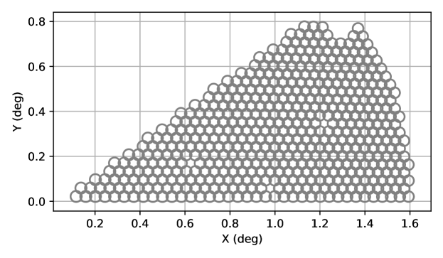
Figure 1: Patrol areas of the 500 fiber positioners of a DESI petal with physical coordinates converted to angles to the center of the field of view. One can see that the patrol areas from adjacent fibers overlap.

4.1.2 Characterization

We intend to evaluate the contribution of the sky model noise to the Ly$\alpha$ auto-correlation of the DESI Y1 sample. As stated in the introduction of §4, we start from the set of forest $\{\delta_{q}\}$ obtained for this sample. This data set consists of lines of sight from more than 450,000 quasars, the detailed of which will be published with the Year 1 analysis [47]. We note that the procedure used to extract the $\delta_{q}$ from the spectra is the one presented in [25].

We build a synthetic data set by replacing the original $\delta_{q}$ values of transmitted flux fraction fluctuations by a realization of the sky subtraction residuals while keeping exactly the same weights and sky coordinates. This guarantees that the mock sample will be directly comparable to the true data, in particular in terms of redshift distribution.

The original $\delta_{q}$ vector of each quasar has been calculated starting with the combined spectrum obtained by optimally averaging the spectra of the same quasar from several exposures (up to four exposures to reach full depth in the DESI main survey). As part of the DESI pipeline processing, a sky background spectrum model is derived for each exposure and each of the 30 cameras (considering 3 cameras per DESI spectrograph). Our focus is on the blue cameras spanning the wavelength range 3600–5772 Å, which fully contain the Ly$\alpha$ DESI Y1 sample. The sky background model is composed of a common spectrum applied to all the fibers of a camera, along with corrections on sky lines that are based on templates obtained with a principal component analysis (see [30], Eq. 15). When it comes to the wavelength range used for the Ly$\alpha$ forest, we can ignore those corrections as they affect only the bright oxygen sky line that is masked out.

Consequently, in order to emulate the spectral correlations coming from the sky model noise in each blue camera and exposure, we can simply generate a random realization of the common sky spectrum noise assuming that it follows a Gaussian distribution with zero mean and with the same variance as the one provided by the pipeline for the sky model (which has been modeled in great details, see Equation 16 of [30]), all the while being uncorrelated from one wavelength bin to the next. We apply to the noise vectors the flux calibration derived from standard stars for the same exposure and camera, such that the resulting $\delta F_{sky}(\lambda)$ have the same units as the calibrated quasar spectra. One realization of $\delta F_{sky}(\lambda)$ applies to all of the fibers from the same camera and the same exposure.

Then, for each Ly$\alpha$ line of sight, we identify the list of exposures and cameras that were used to produce the combined sky-subtracted spectrum, we average the random sky noise spectra of those exposures and cameras, denoted $\left<\delta F_{sky}\right>_{q}$ in what follows, and then we replace the original Ly$\alpha$ $\delta_{q}$ by this average sky noise spectrum divided by the quasar continuum used to derive the $\delta_{q}$ and including the mean flux transmission fraction. In other words, we have

$$\delta^{s}_{q}(\lambda)\equiv\frac{\left<\delta F_{sky}\right>_{q}}{C_{q}\overline{F}}(\lambda).$$ (4.1)

The next step is to apply the projection that removes the mean and slope from each line of sight to get the $\hat{\delta}^{s}_{q}$. This step is part of the estimator of the correlation function [48, 25]. In our case, it emulates the effect of continuum fitting.

The auto-correlation of this mock data set $\{\hat{\delta}^{s}_{q}\}$ gives us the contribution from the sky noise to the Ly$\alpha$ correlation function. It is represented on Figure 2. One can see that the signal is mostly limited to the first $r_{\parallel}$ bin as expected from this white noise simulation (i.e. simulation of the uncorrelated noise between pixels). The extension to larger values of $r_{\parallel}$ is entirely caused by the distortion due to the effect of continuum fitting (actually the projection for our simplified mock data set).

Along $r_{\perp}$, one can see that the signal does not extend beyond $\sim 100$ $h^{-1}$Mpc. It is as expected. We derive a more predictive model in the next section.

It is worth noting from Eq. 4.1 that the amplitude of this sky noise correlation function will decrease with increasing survey depth (or number of observations per target for DESI) and the target brightness. The data shown here is expected to be a fair estimate of the amplitude of the signal in the DESI Y1 Ly$\alpha$ auto-correlation.

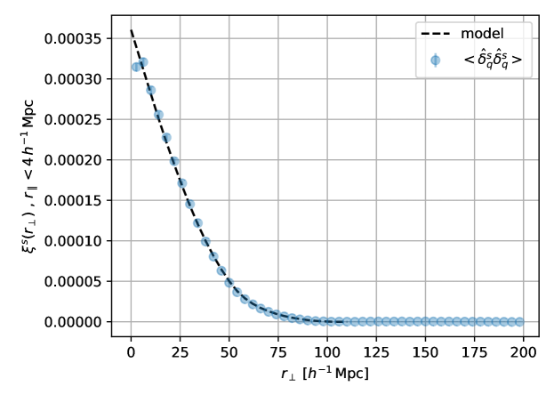
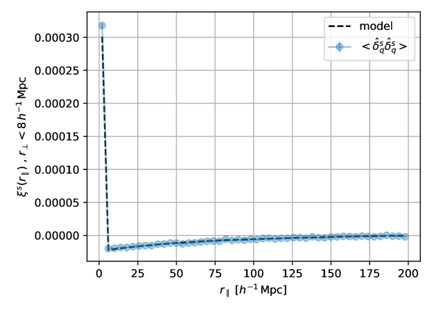
Figure 2: Expected contribution of the sky model noise to the DESI Y1 Ly$\alpha$ auto-correlation. The blue dots are the measured correlation function from the mock $\delta^{s}_{q}$ data set which emulates the sky model noise contibution to the Ly$\alpha$ forests, and the dashed curve is the model described in §4.1.3 derived from the geometry of a DESI petal and accounting for the distortion induced by continuum fitting. The top plot is the correlation as a function of the transverse separation $r_{\perp}$ for the first $r_{\parallel}$ bin which includes pairs at the same wavelength and hence directly the white noise contribution. The bottom plot is the correlation as a function of $r_{\parallel}$ averaged over the first two bins of $r_{\perp}$ highlighting the effect of continuum fitting for values of $r_{\parallel}>0$.

4.1.3 Modeling the noise correlation function

Because the sky model noise is not correlated as a function of wavelength in first approximation – at least it is the case in the emulation presented above – any non-null correlation for $r_{\parallel}>0$ must be the consequence of the continuum fitting. As mentioned in Section 3, this effect on the correlation function is characterized by a distortion matrix $D$ which applies to the model of the undistorted 2D correlation function when represented as an array of values in bins of $(r_{\parallel},r_{\perp})$. The undistorted noise correlation function is of the form $\xi_{noise}(r_{\parallel},r_{\perp})=\delta^{K}(r_{\parallel})f(r_{\perp})$. The function $f(r_{\perp})$ is proportional to the probability that at a pair of measurements separated by $r_{\perp}$ is coming from spectra observed in the same petal and exposure. It can be derived from the geometry of a petal and the fiducial cosmology used to convert angles and redshifts into distances.

A DESI petal is represented in Figure 1 with the circular patrol area of its 500 fiber positioners. The probability of a pair of random coordinates to be accessible by fibers in the same petal can be computed numerically for this data, picking an arbitrary normalization. The angular separation can be converted to comoving separation provided a fiducial cosmology (given above) and a fiducial redshift, here $z_{fid}=2.4$. The difference between this value of $z_{fid}$ and the effective redshift of the final DESI Y1 sample is smaller than 0.1. This is close enough for the level of precision required with the current data sample.

We choose to normalize the model such that $\xi_{noise}(r_{\parallel}=0,r_{\perp}=0)\equiv 1$ and fit a multiplicative amplitude $a_{noise}$ to the measurements. This gives the model represented as a black dashed curve in the top panel of Figure 2, with a fitted amplitude $a_{noise}\simeq 3.8\times 10^{-4}$. The bottom panel shows the additional effect of the distortion matrix. The figure highlights the excellent agreement between the model and the mock data. In an earlier work, [26] used a second order polynomial of $r_{\perp}$ instead of the numerical computation presented here. Both forms are close but we recommend using the more accurate numerical result of this paper in future works. It is included in the vega software used for the fit of DESI data.

4.2 Spectrophotometric calibration uncertainties

4.2.1 Description

Spectro-photometric (or flux) calibration uncertainties introduce correlations in the quasar spectra and therefore in the Lyman-$\alpha$ auto-correlation. In DESI, as in previous surveys like BOSS/eBOSS, the flux calibration is derived from a comparison of the measured spectra of standard stars with stellar models (see [30] §4.8 and §4.9). For DESI, this is performed independently from petal to petal as is the case for the sky subtraction. The precision of the fit of stellar models can be evaluated by comparing the measured colors (as a difference of magnitudes) of stars from the imaging survey used for targeting with the synthetic colors derived from the stellar models. We find in DESI a typical RMS value of 0.02 in $g-r$ per star. Given that about 10 fibers are pointed to standard stars per petal, this corresponds, after averaging, to a calibration uncertainty of about 0.6% at a wavelength scale of about 2000 Å, which is the typical width of a filter. Because we fit a normalization and slope per forest, as explained in Section 3, any calibration error at a scale larger than 500 Å is suppressed. On the other hand the contribution of the measurement white noise to the calibration, at a scale given by the spectral pixel size of 0.8 Å, would appear like the sky noise described in the previous section. Thus we are concerned by the noise introduced at intermediate scales and caused by modeling errors of the standard stars absorption lines, or on the contrary, caused by variations of the throughput during the night and from fiber to fiber. Of concern, for instance, is the variation with humidity of the position of a transmission dip in the spectrographs collimator mirror reflectivity around 4400 Å ([28]).

4.2.2 Characterization

We aim at estimating the flux calibration errors while preserving their correlation across wavelengths.

Calibration vectors $C_{p,e}(\lambda)$ (as defined by Eq. 17 of [30]) translate flat-fielded and sky-subtracted fiber spectra in units of electrons$\cdot$Å^-1 into spectral energy densities in units of ergs$\cdot$s^-1$\cdot$cm^-2$\cdot$Å^-1. They are determined for each petal $p$ and exposure $e$, from the ratio of the measured counts to expected flux of calibration stars. We use the average ratio over all of the calibration stars measured in the same petal. About 10 calibration stars are observed per petal. The exact calibration procedure is more complex as it accounts for variations of spectral resolution from one fiber to the next and corrections for variations of fiber acceptance in the focal plane which vary very slowly with wavelength and can be ignored here (see [30] for more details).

Our approach is to use the relative variation of the flux calibration vector $C_{p,e}(\lambda)$ as a measurement of calibration errors. Our objective is to isolate a signal that we think to be null if the calibration step has been done optimally, and non-zero if there are any calibration errors. We will compare different petals and exposures from different tiles and correct for the average effects arising from atmospheric corrections and temporal effects arising from humidity variations, as well as variations from spectrograph to spectrograph.

For that, we start by defining the contrast between the flux calibration vector of a petal and the average over all 10 petals. When comparing different exposures, we only consider exposures of different tiles so as to get a different set of calibration stars. It follows that the variation of calibration from one exposure to the other will account for the errors arising from the stellar model used.

$$\delta C_{p,e}(\lambda)=C_{p,e}/\left<C_{p,e}\right>_{p}(\lambda)-1$$ (4.2)

This quantity removes, to a good approximation, any genuine change in the calibration with exposure time, airmass, sky transparency and seeing.

Then, we look at how $\delta C_{p,e}$ varies from one exposure to the next. The purpose of our approach is to reduce the contribution of the known time-dependent variation of calibration with humidity. As a result, that contribution is minimized when looking at successive exposures. Therefore, the quantity of interest for our study is:

$$\delta C^{\prime}_{p,e}(\lambda)=\frac{1}{\sqrt{2}}\left(\delta C_{p,e}-\delta C_{p,e+1}\right)(\lambda).$$ (4.3)

Let us study the covariance of that quantity. The RMS of the $\delta C^{\prime}$ are shown as a function of wavelength in Figure 3 after subtracting an average over wavelength for each exposure and camera as a first approximation to account for the continuum subtraction. The calibration error is larger at shorter wavelength because of the lower throughput, which results in a larger measurement noise. On top of that, several spikes are present. The largest spike at 5579 Å is caused by the oxygen sky line which is masked out. The broader excess around 4350 Å is caused by the transmission dip. On one hand, the transmission dip naturally induces a higher relative measurement noise caused by the lower throughput at this wavelength. On the other hand, there are actual variations of the throughput from one exposure to the next. One can also see several sharp features that correspond to the Balmer line series and are marked as vertical dashed lines in Figure 3. Those excesses are unambiguously calibration errors. They can be caused by measurement uncertainties in the star spectra simply because the signal to noise is lower at those wavelengths. It can also be caused by errors in the modeling of the stellar atmospheres, a mismatch between the observed and expected resolution of the instrument, or some noise in the measurement of the radial velocities of stars.

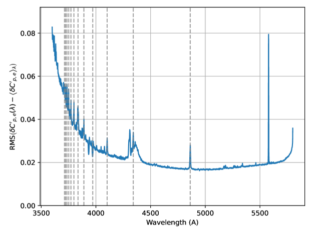
Figure 3: RMS of the spectrophotometric calibration residuals $\delta C^{\prime}_{p,e}(\lambda)$ for the blue cameras after subtracting an average over wavelength for each exposure ($e$) and camera ($p$ for the petal associated to the camera). The latter is done in order to mimic, to first approximation, the effect of continuum fitting. The vertical dashed lines indicate the wavelengths of the Balmer series.

We now compute the 1D correlation function ($\xi^{c}_{1D}$) of the calibration errors as a function of the comoving separation along the line of sight $r_{\parallel}$. We can convert wavelength differences into comoving separations using the Ly$\alpha$ wavelength for redshifts and our fiducial cosmology. This 1D correlation function is given by

$$\xi^{c}_{1D}(r_{\parallel})=\left<\,\delta C^{\prime}_{p,e}(\lambda)\,\delta C^{\prime}_{p,e}(\lambda+\Delta_{\lambda}(\lambda,r_{\parallel}))\,\right>_{p,e,\lambda}$$ (4.4)

where the average is over all petals $p$, exposures $e$, and wavelength $\lambda$, and where $\Delta_{\lambda}(\lambda,r_{\parallel})$ is the wavelength difference that corresponds to the comoving separation $r_{\parallel}$ at the wavelength $\lambda$.

The result is shown in Figure 4. Apart for the peak at 0 separation which corresponds to a white noise term with an RMS of about 0.02, the correlation function is featureless. The shape as a function of $r$ will be different once we account for the Ly$\alpha$ forests specific length, weights and the effect of the projection. Its amplitude will also be reduced when averaged over several exposures.

Figure 4: Average one dimensional auto-correlation function $\xi^{c}_{1D}(r_{\parallel})$ of the spectro-photometric calibration errors $\delta C^{\prime}_{p,e}(\lambda)$ (see equation 4.4).

4.2.3 Calibration noise 2D correlation function

Similarly to the sky subtraction test presented in §4.1.2, we use the actual DESI Y1 Ly$\alpha$ forest data set, keeping all properties including weights but, replacing the $\delta_{q}$ values by random calibration errors. We use directly one of the $\delta C^{\prime}_{p,e}(\lambda)$ array for each petal $p$ and exposure $e$ instead of picking random Gaussian values in order to preserve the correlation across wavelengths. More precisely, for each Ly$\alpha$ line of sight, we identify the list of exposures $\{e\}$ and petals $\{p\}$ that were used to produce the combined quasar spectrum in which the forest is measured, and then we replace the original Ly$\alpha$ $\delta_{q}$ by the average of the calibration errors.

$$\delta^{c}_{q}(\lambda)\equiv\left<\delta C^{\prime}_{p,e}\right>_{q}(\lambda)$$ (4.5)

In the same way that we did for the sky, we apply the projection to obtain the $\{\hat{\delta}^{c}_{q}\}$. Then, we measure their 2D auto-correlation function. The result is shown in Figure 5, where one can see that the contribution of the calibration noise is much smaller than that of the sky model noise. In the lower plot, one can note that the shape of the correlation as a function of $r_{\parallel}$ does not follow that of the sky noise, indicating some genuine correlation as a function of wavelength, but this contribution is very small and can safely be neglected for the Ly$\alpha$ analysis. As an example, at $r_{\parallel}\sim 100$ $h^{-1}$Mpc, the amplitude of the Ly$\alpha$ auto-correlation function is about $2\times 10^{-4}$, when that of the calibration noise is of $2\times 10^{-6}$. Subtracting this contamination to the Ly$\alpha$ auto-correlation function (both in the Lyman-$\alpha$ and Lyman-$\beta$ forest regions) in the DESI Y1 cosmology fit [47] changes the best fit BAO parameters by less than 0.05% and increases the combined $\chi^{2}$ of the fit by about one.

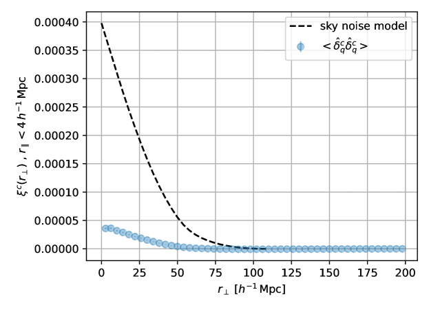
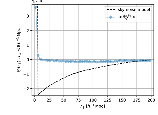
Figure 5: Expected contribution of the spectro-photometric calibration noise to the DESI Y1 Ly$\alpha$ auto-correlation. The blue dots are the measured correlation function from the mock calibration noise contribution $\delta^{c}_{q}$, and the dashed curve is the model described in §4.1.3 for the sky model noise for comparison. The top plot is the correlation as a function of the transverse separation $r_{\perp}$ for the first $r_{\parallel}$ bin, the bottom plot is the correlation as a function of $r_{\parallel}$ averaged over the first two bins of $r_{\perp}$.

4.3 Comparison with BOSS and eBOSS

The SDSS focal plane instrument used for both the BOSS and eBOSS surveys is of comparable angular size to DESI, with a field of view angular diameter of about 3 deg [50]. The focal plane fibers are separated in two halves, each feeding a different spectrograph. As for DESI, the data processing is performed independently for each spectrograph, and this includes the sky and calibration models.

[20] and [24] analysed the BOSS and eBOSS Ly$\alpha$ correlation functions and also found that the noise correlations were dominated by the sky subtraction noise. [20] find a noise correlation in the CIV forest of $2\times 10^{-4}$ in the first separation bin ($r_{\perp},r_{\parallel}<4\,$$h^{-1}$Mpc, see their Figure 8) and [24] find a value of about $5\times 10^{-5}$ in the same bin in the MgII region (see their Figure 9). Those differences are explained by different relative brightness of the quasars compared to the sky level, and variations in the number of fibers allocated for the fit of the sky background. DESI is targeting fainter quasars and only a fraction of them have been observed at full depth in the first year sample, so it is natural that we find a larger contribution of the sky model noise in the DESI Y1 data set.

4.4 Summary

We have identified two sources of correlated noise coming from the data processing pipeline: the sky background model noise and the spectro-photometric calibration noise. The effect of both of those terms on the DESI Year 1 Ly$\alpha$ auto-correlation function have been evaluated. A numeric model of the contribution of the white noise has been proposed. We also find that the component of the calibration noise that is not white noise can be safely neglected in the analysis of the Ly$\alpha$ auto-correlation function. However, we have not modeled all of the possible sources of correlated noise, and specifically for the sky noise, we have not addressed all the sources of noise that are not coming from the model itself. In the following section, we will measure the correlation function of the flux transmission fraction of low redshift quasar spectra, where there is no Ly$\alpha$ forest absorption in order to estimate the combined contribution of all of the sources of correlated noise plus the auto-correlation of foreground absorbers.

5 Astrophysical contaminants

In order to validate the DESI noise correlation function model derived in the previous section, and verify whether it is sub-dominant compared to the cosmological signal, one wants to make a direct and isolated measurement of the spurious correlations arising from the instrument. That requires devising some sort of a null test, i.e. correlating parts of the quasars’s spectra that contain a minimal amount of cosmological signal while retaining all of the instrumental noise.

The difficulty with this comes from the fact that hydrogen is not the only absorber with which the light from the quasar interacts while crossing the universe on its way towards us. Indeed there are irreducible astronomical foreground in the form of metal absorption that make any attempt at a real null test unattainable. As a result, we resort to study the auto-correlations in metal spectral regions of the quasar rest-frame spectrum, redward of the Ly$\alpha$ forest. This gives us the opportunity to measure the combined contamination from correlated noise and foreground absorbers.

5.1 Metal spectral regions

In the rest-frame of a high redshift quasar, foreground absorption features from a given chemical species will appear at shorter wavelength than the corresponding rest-frame emission peak. The metal with the highest rest-frame wavelength will therefore contaminate the regions affected by other metal absorption at smaller rest-frame wavelength, as highlighted on Figure 6. We start by characterizing the auto-correlation of the MgII forest, then the CIV forest and finally the SiIV forest, going from the most pristine region towards increasingly contaminated regions.

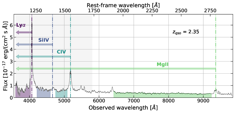
Figure 6: Quasar spectrum at $z=2.35$ displaying several emission lines and the Ly$\alpha$ forest. The Ly$\alpha$ forest is highlighted in purple. The MgII, CIV and SiIV forests are highlighted in various shades of green to blue. MgII absorption span leftward of the MgII peak, contaminating CIV, SiIV, and Ly$\alpha$  forests. CIV absorption span leftward of the CIV doublet, contaminating SIV and Ly$\alpha$  forests. SiIV absorption span leftward of the SiIV peak, contaminating the Ly$\alpha$  forest. The blue spectrograph region is shaded in gray.

Spectral region	$\lambda_{RF}$ range	QSO redshifts
MgII	1920-2760 Å	0.3-2.0
CIV	1420-1520 Å	1.4-3.1
SiIV	1260-1375 Å	1.6-3.6
Ly$\alpha$	1040-1205 Å	2.0-4.5

Table 1: The spectral regions we define and their corresponding quasar rest-frame wavelength ranges. The quasar redshift range is derived for the fixed common observer-frame wavelength range 3600-5772Å (we omit here the additional requirements on the minimal length of a forest which restrict further the redshift range).

We summarize the properties of each metal spectral region in Table 1. The boundaries of the MgII forest are set by the CIII emission line at 1908Å and the MgII emission line at 2796Å  which means we will not get contamination from any IGM absorption at a wavelength shorter than 1920Å in this sample but we expect contamination from larger wavelengths, including MgII. The CIV forest is bounded by the Si IV 1375Å emission line and the CIV 1548Å emission line. It receives contributions from any absorber at $\lambda_{RF}>1375$Å, we expect its auto-correlation to be dominated by CIV absorption, with minor contributions from AlII, AlIII, FeII, MgII (see [51, 52, 53]). Finally, the Si IV forest is bounded by the onset of intervening SiII 1260Å absorption and the SiIV 1394Å emission line. It receives contributions from the same species as the CIV forest, plus OI, SiII, CII and the SiIV lines that we expect to be sub-dominant only to CIV absorption. We note that the SiII 1260Å and other Si lines at shorter wavelength are detected unambiguously and included in the fit of the Ly$\alpha$ auto-correlation as they appears clearly in their cross-correlation with the Ly$\alpha$ absorption (see e.g.  [24]).

5.2 Correlation functions

For each forest, we convert wavelength to redshifts considering the Ly$\alpha$ line in order to emulate correctly how the absorbers contaminate the Ly$\alpha$ forests. This means that we will need to use the metal matrices that encode the transformation from the correct co-moving separation of a pair of absorbers to the incorrect co-moving separation one derives when using the Ly$\alpha$ line to convert wavelength to redshifts (see §3).

We also make sure to use the same distribution of weights as a function of wavelength as in the Ly$\alpha$ forest in each metal spectral region, in order to avoid any bias in the integrated correlation function caused by a redshift evolution of the clustering strength of the absorbers. We use the same terms entering in the definition of the weights as for the DESI Y1 Ly$\alpha$ forest (same values of $\eta$ and $\sigma_{LSS}$ in Eq. 6 of [25]), but we apply different scaling as a function of redshifts in order to compensate for the changes of signal to noise with wavelength for the different quasar samples. The average weights as a function of redshift, before and after this scaling, for all the forests are shown in Figure 7.

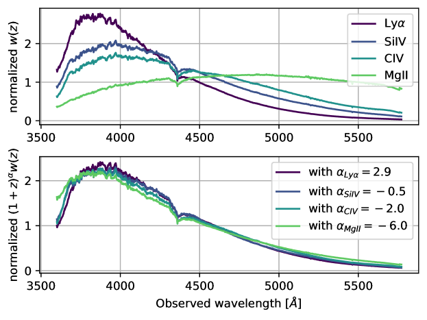
Figure 7: Top: normalized distributions of weights $w(z)$ as a function of wavelength (or equivalently redshift) for the various forests MgII, CIV, SiV and Ly$\alpha$. Bottom: same figure with scaled weights $w^{\prime}(z)\propto(1+z)^{\alpha}\,w(z)$, with $\alpha$ values chosen such that the $w^{\prime}$ weighted average redshift is $\left<z_{Ly\alpha}\right>=2.35$ for all the wavelength regions.

The auto-correlation function of the three forests are shown in Figure 8. The SiIV and CIV correlations as a function of the transverse separation $r_{\perp}$ for the first $r_{\parallel}$ bin show a strong signal at small separation, the signal in the SiIV forest being the largest. The MgII correlation is weaker than the two others.

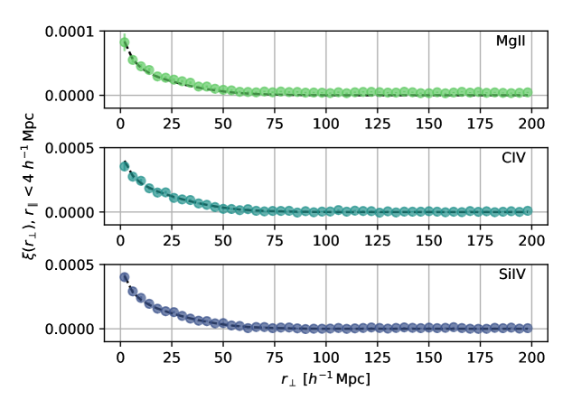
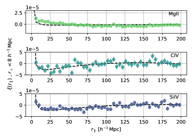
Figure 8: Correlation functions of the MgII, CIV and SiIV forests (colored dots with error-bars) along with their best fit model (black dashed curve). The top plot is the correlation as a function of the transverse separation $r_{\perp}$ for the first $r_{\parallel}$ bin, the bottom plot is the correlation as a function of $r_{\parallel}$ averaged over the first two bins of $r_{\perp}$ (note that the values in the first $r_{\parallel}$ bin are outside of the graph range in the lower plot). The best fit parameters are given in Table 2.

5.3 Metal spectral regions auto-correlation function model and fit

The metal spectral regions correlation functions are fitted with a two component model. The first one is the noise correlation function model $a_{noise}\,\xi_{noise}$ described in §4.1.3, and the second one is the combined signal from the auto-correlation functions of the foreground metal absorbers (hereafter $\xi_{m}$). We consider either a single (effective) absorber or try to isolate the contribution from several of them.

$\xi_{m}$, for a metal absorber ’$m$’, is obtained from the Fourier transform of a power spectrum model ($P_{m}(k,\mu_{k})$, described below), and is then remapped from the true comoving separation (based on the redshifts $z=\lambda/\lambda_{m}-1$, where $\lambda_{m}$ is the metal absorber wavelength) to the assumed comoving separations (based on the redshifts $z=\lambda/\lambda_{Ly\alpha}-1$) with a precomputed metal matrix $M_{m}$ (see §3). Both components are then once again transformed with the distortion matrix $D$ to account for the continuum fitting. Schematically, the correlated signal in a metal spectral region is modeled as

$$\hat{\xi}=D[a_{noise}\,\xi_{noise}+\sum_{m}M_{m}\cdot\xi_{m}]$$ (5.1)

The power spectrum model for the metal absorber $m$ is

$$P_{m}(k,\mu_{k})=b_{m}^{2}(1+\beta_{m}\mu_{k}^{2})^{2}P_{QL}(k)$$ (5.2)

Following the approach of [24], the quasi linear matter power spectrum $P_{QL}(k)$ is derived from the linear matter power spectrum $P_{lin}(k)$ by decoupling and broadening the BAO peak (see their Eq. 28). $P_{lin}(k)$ is precomputed with CAMB [54], for the fiducial cosmology at a fixed reference redshift $z_{ref}$. $P_{QL}(k)$ is then multiplied by a Kaiser term for the redshift space distortions, with the bias parameters $b_{m}$ and $\beta_{m}$. Note that formally, we do not need to include the broadening of the BAO peak in our study since we are focusing on smaller scales. However, in the interest of consistency, we made the choice to use the same model for metals as used in the main Ly$\alpha$  analysis [47].

We now provide details for the metal absorbers considered in each of the metal spectral regions.

• For the MgII spectral region, we consider only the MgII absorption and adopt a single effective rest-frame wavelength $\lambda_{MgII}=2799$Å to account for the combined effect of the absorption occuring at 2796Å, 2804Å, and 2853Å (see [24]). As we will see in the next section, the auto-correlation of the MgII spectral region is probably contaminated by other foreground absorbers, so we will fit for an effective bias $b^{eff}_{MgII}$, with the subscript MgII to note that we use the MgII wavelength to compute the metal matrix, but keeping in mind that this bias is probably the result of the combined effect of multiple absorbers.

• For the CIV spectral region, we consider an effective CIV rest-frame wavelength $\lambda_{CIV}=1549.1$Å. It is actually a doublet of lines at $1548.2$Å and $1550.8$Å. As previously done in [55] and [56] we do not try to differentiate them here. We consider only this absorber in the fit because it dominates the others, but the CIV spectral region auto-correlation function also receives contributions from MgII and other foreground absorbers. As a consequence, we will fit for a single effective bias $b^{eff}_{CIV}$.

• Finally, for the SiIV spectral region, we also consider for our baseline the CIV absorption, fitting again an effective bias $b^{eff}_{CIV}$ that will this time receive an extra contribution from the SiIV absorption. We also test the possibility to model separately the auto-correlation of the SiIV, considering for this an effective wavelength of 1396.8Å (when it is actually a doublet of lines).

For all metal absorbers, we use a redshift space distortion parameter $\beta_{m}=0.5$ following [20].

5.4 Fit results

The fit parameters are the amplitude $a_{noise}$ of the noise correlation function and the bias parameters for the absorbers. The best fit parameters and reduced $\chi^{2}$ values are given for all three metal spectral regions in Table 2. We note that the measured biases and correlated noise amplitudes are quite correlated, with a correlation coefficient close to 0.5. We also obtain different values of the correlated noise amplitude $a_{noise}$ between the spectral regions. This is caused by differences in the continuum level that modulates the sky residual noise (see equation 4.1 where the sky residuals are divided by the continuum).

Spectral region	bias	$a_{noise}\times 10^{4}$	$\chi^{2}/ndf$	$ndf$
Mg II	$b^{eff}_{MgII}=-0.0053\pm 0.0005$	$0.42\pm 0.01$	1.54	1588
CIV	$b^{eff}_{CIV}=-0.0182\pm 0.0015$	$2.73\pm 0.09$	1.06	1588
SiIV	$b^{eff}_{CIV}=-0.0191\pm 0.0012$	$2.57\pm 0.04$	1.11	1588

Table 2: Auto-correlation function fit parameters for the metal spectral regions. $\delta_{q}$ weights have been rescaled as a function of wavelength in order to obtain for all forests the same weighted mean wavelength as for the Ly$\alpha$ forest.

We measure a relatively small but significant signal in the MgII spectral region. The fit result gives an effective bias that is larger than the MgII bias derived from the cross-correlation with quasars. [24] obtain from the cross-correlation a combined MgII bias of $-0.0025\pm 0.0002$ while we measure from the auto-correlation a bias $b^{eff}_{MgII}=-0.0053\pm 0.0005$. We also note that the reduced $\chi^{2}$ of our fit is larger than one. This suggests that the model is incomplete and that there are other contributions to the MgII spectral region signal. We do not try to identify them in this paper because it is a very small signal (four times smaller that the combined effect of CIV and SiIV), but we note that this measurement provides us with a good estimate of the contribution of unidentified contaminants to the Ly$\alpha$ forest (among which are interstellar medium absorbers for instance, see [57]).

For the CIV and SiIV spectral regions, we obtain better reduced $\chi^{2}$ because the CIV and SiIV signals dominate and the uncertainties are larger. The latter is due in part to the contribution of CIV and SiIV to the signal variance, and in part to the length of the forests and quasar redshift distributions. In the CIV spectral region, we obtain a effective bias $b^{eff}_{CIV}=-0.0182\pm 0.0015$. One can estimate the true CIV bias by subtracting the contribution of MgII and other contaminants obtained with the fit of the MgII spectral region. To a good approximation, this consists in subtracting quadratically the two effective biases while taking into account the change of growth of structure between the redshifts of the two absorbers,

$$\left(b_{CIV}\right)^{2}\simeq\left(b_{CIV}^{eff}\right)^{2}-\left(b_{MgII}^{eff}\right)^{2}\frac{D^{2}(z_{MgII})}{D^{2}(z_{CIV})}$$ (5.3)

where $D(z)$ is the large scale structure growth factor at the redshift $z$. This gives $b_{CIV}=-0.016\pm 0.002$, for $z_{MgII}=0.455$ and $z_{CIV}=1.63$. This result is marginally compatible with the CIV bias measured from the cross-correlation of CIV with quasars. For instance, [56] report a value of $b_{CIV}(1+\beta_{CIV})=-0.0183\pm 0.0014$ at $z=2$ from the SDSS BOSS/eBOSS data sample. This gives $b_{CIV}=-0.012\pm 0.001$ for our choice of $\beta_{CIV}=0.5$.

This difference of bias is only barely significant, but if true, we are then left with two hypotheses: i) there are other sources of correlated noise in the DESI data set that are not accounted for with our simple model, ii) the cross-correlation of quasars and CIV absorption is driven not only by large-scale structure but also by an astrophysical connection between the quasar positions and the CIV absorption strength.

In order to test the first hypothesis and verify that we have been able to separate the contribution of the noise correlations from that of genuine astrophysical sources, we repeat the measurement of the CIV forest auto-correlation by considering only $\delta_{q}$ pairs from quasar spectra recorded in different spectrographs (corresponding to different petals of the focal plane). This excludes most sources of noise coming from the data processing pipeline because most of the data reduction is performed independently for each spectrograph. The resulting correlation is compared to the measurement with the full data set in Figure 9. As expected, we find a much smaller signal when correlating spectra from different spectrographs and we further find that the measured correlation is consistent with the modeled CIV absorber auto-correlation (without the noise correlation). When we fit this correlation, we obtain $b^{eff}_{CIV}=-0.0183\pm 0.0015$ and $a_{noise}=0.4\pm 0.1$. The bias is the same as with the full data set while the noise correlation is seven times smaller. This result demonstrates that we are able to separate the instrumental noise correlation from the astrophysical signal in the metal spectral regions correlation fit, and that our noise correlation model is a good match to the data. As a cross-check, we also measure the CIV auto-correlation function when considering only $\delta_{q}$ pairs from quasar spectra recorded in different nights, and we find a similar result. This additional test shows that there is no evidence of correlated noise coming from the daily calibrations (CCD bias levels, spectrograph PSF, fiber flat fielding on the dome screen, see [30]) or any unanticipated variation of the instrument response from night to night.

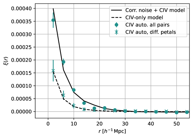
Figure 9: Auto-correlation function as a function of separation in the CIV forest including all $\delta_{q}$ pairs (dots with error bars) or only those from different petals and exposures (stars), along with the best fit model from the fit of the full data set (solid curve, see Eq. 5.1), and the contribution from the CIV absorber correlation only (dashed curve, corresponding to the term $DM_{m}\xi_{m}$ in the same equation).

We can also compare the amplitude of the noise correlation obtained in this fit of the CIV forest with the prediction presented in §4.1 for the Ly$\alpha$ forest. A fit of the emulated Ly$\alpha$ forest sky noise correlation shown in Figure 2 gives a noise correlation amplitude $a_{noise}(\mathrm{Ly}\alpha)\sim 3.8\times 10^{-4}$. Now we measure on average a larger quasar continuum in the CIV forest than in the Ly$\alpha$ forest, with a ratio $C_{CIV}/C_{\mathrm{Ly}\alpha}$=1.13, so we expect a smaller noise correlation amplitude in the CIV forest after the flux is divided by the continuum. Numerically, this gives $a_{noise}(CIV)\sim a_{noise}(\mathrm{Ly}\alpha)(C_{\mathrm{Ly}\alpha}/C_{CIV})^{2}\sim 3.0\times 10^{-4}$. This is consistent within 10% with the measurement reported in Table 2.

Concerning our second hypothesis, a natural source of correlation between the CIV strength and quasar positions is the inhomogeneity in the distribution of carbon ionizing photons arising from quasars. Quasars are thought to be a major source of the photons that maintain the IGM ionized but the mean free path of hydrogen ionizing photons is very large ($>100\ h^{-1}$ Mpc, see [58]). On the other hand the mean free path of carbon (and silicon) ionising photons can be very much shorter due to helium-II reionization effects [59, 60, 61]. [62] probes the inhomogeneity of metal species such as CIV with respect to 3D proximity to quasars using eBOSS quasar spectra. They find some evidence of variation of the CIV bias with the distance from quasars though direct comparisons of their measurements and ours are non-trivial at this stage.

Looking now at the SiIV spectral region, we measure a larger CIV effective bias $b_{CIV}^{eff}=-0.0191\pm 0.0012$. A larger bias is expected because it includes the contribution of SiIV absorbers in addition to the CIV, MgII and other unidentified weak absorbers. This increase in amplitude is qualitatively consistent with results on the 1D Ly$\alpha$ power spectrum (see e.g. Fig. 18 of [63] or more recently Fig. 9 of [64]). We can not reliably isolate the SiIV contribution when looking at the combined auto-correlation without additional information. One possibility is to add a prior on the CIV effective bias $b^{eff}_{CIV}$ from the measurement obtained in the CIV forest.

When refitting the SiIV forest with this method, we obtain $b_{SiIV}=-0.006\pm 0.007$ when assuming a prior $b^{eff}_{CIV}=-0.0182\pm 0.0015$. The quadratic sum of those two numbers, accounting for the change of growth factor, is consistent with the value obtained when fitting only the CIV effective bias. We also find that there is no gain in the quality of the fit (only 0.1 change in the fit $\chi^{2}$) when treating separately the SiIV absorber. In consequence, it is equivalent to consider one or two absorbers in the modeling of the auto-correlation function.

6 Summary

In this paper, we have studied the main contaminants of the Ly$\alpha$ forest auto-correlation function measured with DESI. They can be separated in two broad catagories: correlated residuals in the spectra introduced by the data processing pipeline, and astrophysical foreground absorbers in the intergalactic medium and interstellar medium (ISM). We have first characterized the correlated noise introduced by the data processing. The main contribution is the statistical noise from the sky background model that is subtracted to all spectra from the same exposure and spectrograph. We have estimated the signal level by emulating the noise in a mock data set, and we have proposed a simple model to account for it (see Fig. 2). The second source of correlated noise comes from the spectrophotometric calibration uncertainties. We have characterized it by measuring the changes in calibration from one exposure to the next and one spectrograph compared to the others. We have found that this contribution is 10 times smaller and can be neglected (see Fig. 5). This measurement includes the calibration errors introduced by the fit of standard stars.

We have then measured the auto-correlation function of the transmitted flux fraction fluctuation ($\delta_{q}$) in various regions of the quasar rest-frame spectra (Fig 6). We considered only forests with wavelength larger than the quasar Ly$\alpha$ emission line; this ensures that the signal we measure is deprived from Ly$\alpha$ absorption, but we have at the same time considered data in the same observer frame wavelength as the Ly$\alpha$ forest, with the same relative weights as a function of wavelength.

We have looked at the auto-correlations of the MgII, CIV ans SiIV spectral regions, fitting each of them with a two component model composed of the noise correlation model and a metal absorber auto-correlation function. We measure increasing values of the absorber bias for each spectral region reflecting the accumulated effect of metal absorbers (MgII, CIV and then SiIV) when probing higher redshifts. We do not obtain a good fit in the MgII region probably because of other unidentified contaminants (for instance in the ISM as studied by [57]). The signal is however four times smaller than the contributions of CIV and SiIV so we did not investigate this in more detail. On the contrary, we obtain good fits in the CIV and SiIV regions. We have further demonstrated the validity of this approach by measuring the auto-correlation using pairs of quasar spectra from different spectrographs where only the astrophysical signal was measured (see Fig. 9). We measure a combined absorber bias $b^{eff}_{CIV}=-0.0191\pm 0.0015$, with $\beta_{CIV}=0.5$. The correlated noise amplitude varies with the data set but can easily be separated from the astrophysical signal in a 2D correlation function. It is reassuring to note that for DESI the contamination from the instrumental effects is very small. The correlated noise signal is featureless at $r_{\parallel}>4$ $h^{-1}$Mpc and about 40 times smaller than the Ly$\alpha$ signal at the BAO scale. We propose to use this two component contamination model when analysing the DESI Lyman-$\alpha$ auto-correlation function.

Appendix A Author Affiliations

¹Lawrence Berkeley National Laboratory, 1 Cyclotron Road, Berkeley, CA 94720, USA

²IRFU, CEA, Université Paris-Saclay, F-91191 Gif-sur-Yvette, France

³Department of Physics and Astronomy, The University of Utah, 115 South 1400 East, Salt Lake City, UT 84112, USA

⁴Center for Cosmology and AstroParticle Physics, The Ohio State University, 191 West Woodruff Avenue, Columbus, OH 43210, USA

⁵NASA Einstein Fellow

⁶Institut de F’isica d’Altes Energies (IFAE), The Barcelona Institute of Science and Technology, Campus UAB, 08193 Bellaterra Barcelona, Spain

⁷Institut de Física d’Altes Energies (IFAE), The Barcelona Institute of Science and Technology, Campus UAB, 08193 Bellaterra Barcelona, Spain

⁸Department of Physics & Astronomy, University College London, Gower Street, London, WC1E 6BT, UK

⁹Departamento de Física, Universidad de Guanajuato - DCI, C.P. 37150, Leon, Guanajuato, México

¹⁰Department of Astronomy, The Ohio State University, 4055 McPherson Laboratory, 140 W 18th Avenue, Columbus, OH 43210, USA

¹¹Department of Physics, The Ohio State University, 191 West Woodruff Avenue, Columbus, OH 43210, USA

¹²The Ohio State University, Columbus, 43210 OH, USA

¹³Instituto de Física, Universidad Nacional Autónoma de México, Cd. de México C.P. 04510, México

¹⁴Aix Marseille Univ, CNRS, CNES, LAM, Marseille, France

¹⁵Departament de Física, EEBE, Universitat Politècnica de Catalunya, c/Eduard Maristany 10, 08930 Barcelona, Spain

¹⁶Aix Marseille Univ, CNRS/IN2P3, CPPM, Marseille, France

¹⁷Université Clermont-Auvergne, CNRS, LPCA, 63000 Clermont-Ferrand, France

¹⁸Sorbonne Universit’e, CNRS/IN2P3, Laboratoire de Physique Nucl’eaire et de Hautes Energies (LPNHE), FR-75005 Paris, France

¹⁹IRFU, CEA, Universit’e Paris-Saclay, F-91191 Gif-sur-Yvette, France

²⁰University Observatory, Faculty of Physics, Ludwig-Maximilians-Universität, Scheinerstr. 1, 81677 München, Germany

²¹Excellence Cluster ORIGINS, Boltzmannstrasse 2, D-85748 Garching, Germany

²²Physics Dept., Boston University, 590 Commonwealth Avenue, Boston, MA 02215, USA

²³Department of Physics and Astronomy, University of California, Irvine, 92697, USA

²⁴SLAC National Accelerator Laboratory, Menlo Park, CA 94305, USA

²⁵Kavli Institute for Particle Astrophysics and Cosmology, Stanford University, Menlo Park, CA 94305, USA

²⁶Observatorio Astronómico, Universidad de los Andes, Cra. 1 No. 18A-10, Edificio H, CP 111711 Bogotá, Colombia

²⁷Departamento de Física, Universidad de los Andes, Cra. 1 No. 18A-10, Edificio Ip, CP 111711, Bogotá, Colombia

²⁸Institut d’Estudis Espacials de Catalunya (IEEC), 08034 Barcelona, Spain

²⁹Institute of Cosmology and Gravitation, University of Portsmouth, Dennis Sciama Building, Portsmouth, PO1 3FX, UK

³⁰Institute of Space Sciences, ICE-CSIC, Campus UAB, Carrer de Can Magrans s/n, 08913 Bellaterra, Barcelona, Spain

³¹Consejo Nacional de Ciencia y Tecnología, Av. Insurgentes Sur 1582. Colonia Crédito Constructor, Del. Benito Juárez C.P. 03940, México D.F. México

³²Fermi National Accelerator Laboratory, PO Box 500, Batavia, IL 60510, USA

³³Department of Astrophysical Sciences, Princeton University, Princeton NJ 08544, USA

³⁴NSF NOIRLab, 950 N. Cherry Ave., Tucson, AZ 85719, USA

³⁵Department of Physics, Southern Methodist University, 3215 Daniel Avenue, Dallas, TX 75275, USA

³⁶Sorbonne Université, CNRS/IN2P3, Laboratoire de Physique Nucléaire et de Hautes Energies (LPNHE), FR-75005 Paris, France

³⁷Departament de Física, Serra Húnter, Universitat Autònoma de Barcelona, 08193 Bellaterra (Barcelona), Spain

³⁸Institució Catalana de Recerca i Estudis Avançats, Passeig de Lluís Companys, 23, 08010 Barcelona, Spain

³⁹Department of Astronomy, Tsinghua University, 30 Shuangqing Road, Haidian District, Beijing, China, 100190

⁴⁰Department of Physics and Astronomy, Siena College, 515 Loudon Road, Loudonville, NY 12211, USA

⁴¹Department of Physics and Astronomy, University of Sussex, Brighton BN1 9QH, U.K

⁴²Department of Physics & Astronomy, University of Wyoming, 1000 E. University, Dept. 3905, Laramie, WY 82071, USA

⁴³National Astronomical Observatories, Chinese Academy of Sciences, A20 Datun Rd., Chaoyang District, Beijing, 100012, P.R. China

⁴⁴Instituto Avanzado de Cosmología A. C., San Marcos 11 - Atenas 202. Magdalena Contreras, 10720. Ciudad de México, México

⁴⁵Department of Physics and Astronomy, University of Waterloo, 200 University Ave W, Waterloo, ON N2L 3G1, Canada

⁴⁶Perimeter Institute for Theoretical Physics, 31 Caroline St. North, Waterloo, ON N2L 2Y5, Canada

⁴⁷Waterloo Centre for Astrophysics, University of Waterloo, 200 University Ave W, Waterloo, ON N2L 3G1, Canada

⁴⁸University of California, Berkeley, 110 Sproul Hall #5800 Berkeley, CA 94720, USA

⁴⁹Space Sciences Laboratory, University of California, Berkeley, 7 Gauss Way, Berkeley, CA 94720, USA

⁵⁰Department of Physics, Kansas State University, 116 Cardwell Hall, Manhattan, KS 66506, USA

⁵¹Department of Physics and Astronomy, Sejong University, Seoul, 143-747, Korea

⁵²CIEMAT, Avenida Complutense 40, E-28040 Madrid, Spain

⁵³Department of Physics, University of Michigan, Ann Arbor, MI 48109, USA

⁵⁴University of Michigan, Ann Arbor, MI 48109, USA

⁵⁵Department of Physics & Astronomy, Ohio University, Athens, OH 45701, USA

References

- [1] A.G. Riess, A.V. Filippenko, P. Challis, A. Clocchiatti, A. Diercks, P.M. Garnavich et al., Observational evidence from supernovae for an accelerating universe and a cosmological constant, The Astronomical Journal 116 (1998) 1009.
- [2] S. Perlmutter, G. Aldering, M.D. Valle, S. Deustua, R.S. Ellis, S. Fabbro et al., Discovery of a supernova explosion at half the age of the universe, Nature 391 (1998) 51.
- [3] J.A. Frieman, M.S. Turner and D. Huterer, Dark energy and the accelerating universe, Annual Review of Astronomy and Astrophysics 46 (2008) 385 [https://doi.org/10.1146/annurev.astro.46.060407.145243].
- [4] D.J. Eisenstein, H.-J. Seo and M. White, On the robustness of the acoustic scale in the low-redshift clustering of matter, The Astrophysical Journal 664 (2007) 660.
- [5] D.J. Eisenstein, I. Zehavi, D.W. Hogg, R. Scoccimarro, M.R. Blanton, R.C. Nichol et al., Detection of the baryon acoustic peak in the large-scale correlation function of SDSS luminous red galaxies, The Astrophysical Journal 633 (2005) 560.
- [6] W.J. Percival, B.A. Reid, D.J. Eisenstein, N.A. Bahcall, T. Budavari, J.A. Frieman et al., Baryon acoustic oscillations in the Sloan Digital Sky Survey Data Release 7 galaxy sample, Monthly Notices of the Royal Astronomical Society 401 (2010) 2148 [https://academic.oup.com/mnras/article-pdf/401/4/2148/3901461/mnras0401-2148.pdf].
- [7] A.J. Ross, L. Samushia, C. Howlett, W.J. Percival, A. Burden and M. Manera, The clustering of the SDSS DR7 main Galaxy sample – I. A 4 per cent distance measure at z = 0.15, Monthly Notices of the Royal Astronomical Society 449 (2015) 835 [https://academic.oup.com/mnras/article-pdf/449/1/835/13767551/stv154.pdf].
- [8] W.J. Percival, C.M. Baugh, J. Bland-Hawthorn, T. Bridges, R. Cannon, S. Cole et al., The 2dF Galaxy Redshift Survey: the power spectrum and the matter content of the Universe, Monthly Notices of the Royal Astronomical Society 327 (2001) 1297 [https://academic.oup.com/mnras/article-pdf/327/4/1297/3279954/327-4-1297.pdf].
- [9] S. Cole, W.J. Percival, J.A. Peacock, P. Norberg, C.M. Baugh, C.S. Frenk et al., The 2dF Galaxy Redshift Survey: power-spectrum analysis of the final data set and cosmological implications, Monthly Notices of the Royal Astronomical Society 362 (2005) 505 [https://academic.oup.com/mnras/article-pdf/362/2/505/6155670/362-2-505.pdf].
- [10] C. Blake, T. Davis, G.B. Poole, D. Parkinson, S. Brough, M. Colless et al., The WiggleZ Dark Energy Survey: testing the cosmological model with baryon acoustic oscillations at z= 0.6, MNRAS 415 (2011) 2892 [1105.2862].
- [11] F. Beutler, C. Blake, M. Colless, D.H. Jones, L. Staveley-Smith, L. Campbell et al., The 6dF Galaxy Survey: baryon acoustic oscillations and the local Hubble constant, Monthly Notices of the Royal Astronomical Society 416 (2011) 3017 [https://academic.oup.com/mnras/article-pdf/416/4/3017/2985042/mnras0416-3017.pdf].
- [12] L. Anderson, É. Aubourg, S. Bailey, F. Beutler, V. Bhardwaj, M. Blanton et al., The clustering of galaxies in the SDSS-III Baryon Oscillation Spectroscopic Survey: baryon acoustic oscillations in the Data Releases 10 and 11 Galaxy samples, Monthly Notices of the Royal Astronomical Society 441 (2014) 24 [https://academic.oup.com/mnras/article-pdf/441/1/24/3007885/stu523.pdf].
- [13] K.S. Dawson, J.-P. Kneib, W.J. Percival, S. Alam, F.D. Albareti, S.F. Anderson et al., The SDSS-IV Extended Baryon Oscillation Spectroscopic Survey: Overview and Early Data, AJ 151 (2016) 44 [1508.04473].
- [14] S. Alam, M. Aubert, S. Avila, C. Balland, J.E. Bautista, M.A. Bershady et al., Completed SDSS-IV extended Baryon Oscillation Spectroscopic Survey: Cosmological implications from two decades of spectroscopic surveys at the Apache Point Observatory, Phys. Rev. D 103 (2021) 083533 [2007.08991].
- [15] N.G. Busca, T. Delubac, J. Rich, S. Bailey, A. Font-Ribera, D. Kirkby et al., Baryon acoustic oscillations in the Ly forest of BOSS quasars, A&A 552 (2013) A96 [1211.2616].
- [16] A. Slosar, V. Iršič, D. Kirkby, S. Bailey, N.G. Busca, T. Delubac et al., Measurement of baryon acoustic oscillations in the lyman- forest fluctuations in BOSS data release 9, Journal of Cosmology and Astroparticle Physics 2013 (2013) 026.
- [17] D. Kirkby, D. Margala, A. Slosar, S. Bailey, N.G. Busca, T. Delubac et al., Fitting methods for baryon acoustic oscillations in the lyman- forest fluctuations in BOSS data release 9, Journal of Cosmology and Astroparticle Physics 2013 (2013) 024.
- [18] A. Font-Ribera, D. Kirkby, N. Busca, J. Miralda-Escudé, N.P. Ross, A. Slosar et al., Quasar-lyman-alpha forest cross-correlation from BOSS DR11: Baryon acoustic oscillations, Journal of Cosmology and Astroparticle Physics 2014 (2014) 027.
- [19] T. Delubac, J.E. Bautista, N.G. Busca, J. Rich, D. Kirkby, S. Bailey et al., Baryon acoustic oscillations in the Ly forest of BOSS DR11 quasars, A&A 574 (2015) A59 [1404.1801].
- [20] J.E. Bautista, N.G. Busca, J. Guy, J. Rich, M. Blomqvist, H. du Mas des Bourboux et al., Measurement of baryon acoustic oscillation correlations at z = 2.3 with SDSS DR12 Ly-Forests, A&A 603 (2017) A12 [1702.00176].
- [21] H. du Mas des Bourboux, J.-M. Le Goff, M. Blomqvist, N.G. Busca, J. Guy, J. Rich et al., Baryon acoustic oscillations from the complete SDSS-III Ly-quasar cross-correlation function at z = 2.4, A&A 608 (2017) A130 [1708.02225].
- [22] V. de Sainte Agathe, C. Balland, H. du Mas des Bourboux, N.G. Busca, M. Blomqvist, J. Guy et al., Baryon acoustic oscillations at z = 2.34 from the correlations of Ly absorption in eBOSS DR14, A&A 629 (2019) A85 [1904.03400].
- [23] M. Blomqvist, H. du Mas des Bourboux, N.G. Busca, V. de Sainte Agathe, J. Rich, C. Balland et al., Baryon acoustic oscillations from the cross-correlation of Ly absorption and quasars in eBOSS DR14, A&A 629 (2019) A86 [1904.03430].
- [24] H. du Mas des Bourboux, J. Rich, A. Font-Ribera, V. de Sainte Agathe, J. Farr, T. Etourneau et al., The completed SDSS-IV extended baryon oscillation spectroscopic survey: Baryon acoustic oscillations with ly forests, The Astrophysical Journal 901 (2020) 153.
- [25] C. Ramírez-Pérez, I. Pérez-Ràfols, A. Font-Ribera, M.A. Karim, E. Armengaud, J. Bautista et al., The Lyman- forest catalog from the Dark Energy Spectroscopic Instrument Early Data Release, MNRAS (2023) [2306.06312].
- [26] C. Gordon, A. Cuceu, J. Chaves-Montero, A. Font-Ribera, A.X. González-Morales, J. Aguilar et al., 3D correlations in the Lyman- forest from early DESI data, J. Cosmology Astropart. Phys 2023 (2023) 045 [2308.10950].
- [27] M.M. Pieri, The C iv forest as a probe of baryon acoustic oscillations., MNRAS 445 (2014) L104 [1404.4569].
- [28] DESI Collaboration, B. Abareshi, J. Aguilar, S. Ahlen, S. Alam, D.M. Alexander et al., Overview of the Instrumentation for the Dark Energy Spectroscopic Instrument, AJ 164 (2022) 207 [2205.10939].
- [29] J.H. Silber, P. Fagrelius, K. Fanning, M. Schubnell, J.N. Aguilar, S. Ahlen et al., The robotic multiobject focal plane system of the dark energy spectroscopic instrument (desi), The Astronomical Journal 165 (2022) 9.
- [30] J. Guy, S. Bailey, A. Kremin, S. Alam, D.M. Alexander, C. Allende Prieto et al., The Spectroscopic Data Processing Pipeline for the Dark Energy Spectroscopic Instrument, AJ 165 (2023) 144 [2209.14482].
- [31] E.F. Schlafly, D. Kirkby, D.J. Schlegel, A.D. Myers, A. Raichoor, K. Dawson et al., Survey Operations for the Dark Energy Spectroscopic Instrument, AJ 166 (2023) 259 [2306.06309].
- [32] E. Chaussidon, C. Yèche, N. Palanque-Delabrouille, D.M. Alexander, J. Yang, S. Ahlen et al., Target Selection and Validation of DESI Quasars, arXiv e-prints (2022) arXiv:2208.08511 [2208.08511].
- [33] A.G. Adame, J. Aguilar, S. Ahlen, S. Alam, G. Aldering, D.M. Alexander et al., Validation of the Scientific Program for the Dark Energy Spectroscopic Instrument, AJ 167 (2024) 62 [2306.06307].
- [34] H.K. Herrera-Alcantar, A. Muñoz-Gutiérrez, T. Tan, A.X. González-Morales, A. Font-Ribera, J. Guy et al., Synthetic spectra for Lyman- forest analysis in the Dark Energy Spectroscopic Instrument, arXiv e-prints (2023) arXiv:2401.00303 [2401.00303].
- [35] A.D. Myers, J. Moustakas, S. Bailey, B.A. Weaver, A.P. Cooper, J.E. Forero-Romero et al., The Target-selection Pipeline for the Dark Energy Spectroscopic Instrument, AJ 165 (2023) 50 [2208.08518].
- [36] S.J. Bailey et al., redrock, in prep. (2024) .
- [37] N. Busca and C. Balland, QuasarNET: Human-level spectral classification and redshifting with Deep Neural Networks, arXiv e-prints (2018) arXiv:1808.09955 [1808.09955].
- [38] J. Farr, A. Font-Ribera and A. Pontzen, Optimal strategies for identifying quasars in DESI, J. Cosmology Astropart. Phys 2020 (2020) 015 [2007.10348].
- [39] DESI Collaboration, DESI 2024 II: Sample definitions, characteristics and two-point clustering statistics, in preparation (2024) .
- [40] A. Brodzeller, K. Dawson, S. Bailey, J. Yu, A.J. Ross, A. Bault et al., Performance of the quasar spectral templates for the dark energy spectroscopic instrument, The Astronomical Journal 166 (2023) 66.
- [41] A.R. Bault, D. Kirkby, J. Guy, A. Brodzeller et al., Impact of Systematic Redshift Errors on the Cross-correlation of the Lyman-alpha Forest with Quasars at Small Scales Using DESI Early Data, in prep. (2024) .
- [42] DESI Collaboration, A.G. Adame, J. Aguilar, S. Ahlen, S. Alam, G. Aldering et al., The Early Data Release of the Dark Energy Spectroscopic Instrument, arXiv e-prints (2023) arXiv:2306.06308 [2306.06308].
- [43] K.M. Gorski, E. Hivon, A.J. Banday, B.D. Wandelt, F.K. Hansen, M. Reinecke et al., HEALPix: A framework for high-resolution discretization and fast analysis of data distributed on the sphere, The Astrophysical Journal 622 (2005) 759.
- [44] B. Wang, J. Zou, Z. Cai, J.X. Prochaska, Z. Sun, J. Ding et al., Deep learning of dark energy spectroscopic instrument mock spectra to find damped ly systems, The Astrophysical Journal Supplement Series 259 (2022) 28.
- [45] S. Filbert, P. Martini, K. Seebaluck, L. Ennesser, D.M. Alexander, A. Bault et al., Broad absorption line quasars in the dark energy spectroscopic instrument early data release, 2309.03434.
- [46] L. Ennesser, P. Martini, A. Font-Ribera and I. Perez-Rafols, The impact and mitigation of broad-absorption-line quasars in Lyman-alpha forest correlations, Monthly Notices of the Royal Astronomical Society 511 (2022) 3514 [https://academic.oup.com/mnras/article-pdf/511/3/3514/42571769/stac301.pdf].
- [47] DESI Collaboration, A.G. Adame, J. Aguilar, S. Ahlen, S. Alam, D.M. Alexander et al., DESI 2024 IV: Baryon Acoustic Oscillations from the Lyman Alpha Forest, arXiv e-prints (2024) arXiv:2404.03001 [2404.03001].
- [48] H. du Mas des Bourboux, J. Rich, A. Font-Ribera, V. de Sainte Agathe, J. Farr, T. Etourneau et al., “picca: Package for Igm Cosmological-Correlations Analyses.” Astrophysics Source Code Library, record ascl:2106.018, June, 2021.
- [49] A. Dey, D.J. Schlegel, D. Lang, R. Blum, K. Burleigh, X. Fan et al., Overview of the DESI Legacy Imaging Surveys, AJ 157 (2019) 168 [1804.08657].
- [50] S.A. Smee, J.E. Gunn, A. Uomoto, N. Roe, D. Schlegel, C.M. Rockosi et al., The Multi-object, Fiber-fed Spectrographs for the Sloan Digital Sky Survey and the Baryon Oscillation Spectroscopic Survey, AJ 146 (2013) 32 [1208.2233].
- [51] M.M. Pieri, M.J. Mortonson, S. Frank, N. Crighton, D.H. Weinberg, K.-G. Lee et al., Probing the circumgalactic medium at high-redshift using composite BOSS spectra of strong Lyman forest absorbers, MNRAS 441 (2014) 1718 [1309.6768].
- [52] L. Yang, Z. Zheng, H. du Mas des Bourboux, K. Dawson, M.M. Pieri, G. Rossi et al., Metal Lines Associated with the Ly Forest from eBOSS Data, ApJ 935 (2022) 121 [2206.11385].
- [53] S. Morrison, D. Som, M.M. Pieri, I. Pérez-Ràfols and M. Blomqvist, A Strong Blend in the Morning: Studying the Circumgalactic Medium Before Cosmic Noon with Strong, Blended Lyman- Forest Systems, arXiv e-prints (2023) arXiv:2309.06813 [2309.06813].
- [54] A. Lewis, A. Challinor and A. Lasenby, Efficient Computation of Cosmic Microwave Background Anisotropies in Closed Friedmann-Robertson-Walker Models, ApJ 538 (2000) 473 [astro-ph/9911177].
- [55] S. Gontcho A Gontcho, J. Miralda-Escudé, A. Font-Ribera, M. Blomqvist, N.G. Busca and J. Rich, Quasar – civ forest cross-correlation with sdss dr12, Monthly Notices of the Royal Astronomical Society 480 (2018) 610–622.
- [56] M. Blomqvist, M.M. Pieri, H. du Mas des Bourboux, N. G. Busca, A. Slosar, J.E. Bautista et al., The triply-ionized carbon forest from eboss: cosmological correlations with quasars in sdss-iv dr14, Journal of Cosmology and Astroparticle Physics 2018 (2018) 029–029.
- [57] Y. Vadai, D. Poznanski, D. Baron, P.E. Nugent and D. Schlegel, The effect of interstellar absorption on measurements of the baryon acoustic peak in the Lyman forest, MNRAS 472 (2017) 799 [1705.03190].
- [58] G.C. Rudie, C.C. Steidel, A.E. Shapley and M. Pettini, The Column Density Distribution and Continuum Opacity of the Intergalactic and Circumgalactic Medium at Redshift langzrang = 2.4, ApJ 769 (2013) 146 [1304.6719].
- [59] A. Songaila and L.L. Cowie, Metal enrichment and Ionization Balance in the Lyman Alpha Forest at Z = 3, AJ 112 (1996) 335 [astro-ph/9605102].
- [60] M.L. Giroux and J.M. Shull, The Influence of the Photoionizing Radiation Spectrum on Metal-Line Ratios in Ly(alpha) Forest Clouds, AJ 113 (1997) 1505 [astro-ph/9701160].
- [61] I.I. Agafonova, S.A. Levshakov, D. Reimers, C. Fechner, D. Tytler, R.A. Simcoe et al., Spectral shape of the UV ionizing background and He II absorption at redshifts 1.8 ¡ z ¡ 2.9, A&A 461 (2007) 893 [astro-ph/0610442].
- [62] S. Morrison, M.M. Pieri, D. Som and I. Pérez-Ràfols, Probing large-scale UV background inhomogeneity associated with quasars using metal absorption, MNRAS 506 (2021) 5750 [2012.00772].
- [63] N. Palanque-Delabrouille, C. Yèche, A. Borde, J.-M. Le Goff, G. Rossi, M. Viel et al., The one-dimensional Ly forest power spectrum from BOSS, A&A 559 (2013) A85 [1306.5896].
- [64] C. Ravoux, M.L. Abdul Karim, E. Armengaud, M. Walther, N.G. Karaçaylı, P. Martini et al., The Dark Energy Spectroscopic Instrument: one-dimensional power spectrum from first Ly forest samples with Fast Fourier Transform, MNRAS 526 (2023) 5118 [2306.06311].