DESI 2024 III: Baryon Acoustic Oscillations from Galaxies and Quasars

Abstract

We present the DESI 2024 galaxy and quasar baryon acoustic oscillations (BAO) measurements using over 5.7 million unique galaxy and quasar redshifts in the range $0.1<z<2.1$. Divided by tracer type, we utilize 300,017 galaxies from the magnitude-limited Bright Galaxy Survey with $0.1<z<0.4$, 2,138,600 Luminous Red Galaxies with $0.4<z<1.1$, 2,432,022 Emission Line Galaxies with $0.8<z<1.6$, and 856,652 quasars with $0.8<z<2.1$, over a $\sim 7,500$ square degree footprint. The analysis was blinded at the catalog-level to avoid confirmation bias. All fiducial choices of the BAO fitting and reconstruction methodology, as well as the size of the systematic errors, were determined on the basis of the tests with mock catalogs and the blinded data catalogs. We present several improvements to the BAO analysis pipeline, including enhancing the BAO fitting and reconstruction methods in a more physically-motivated direction, and also present results using combinations of tracers. We employ a unified BAO analysis method across all tracers. We present a re-analysis of SDSS BOSS and eBOSS results applying the improved DESI methodology and find scatter consistent with the level of the quoted SDSS theoretical systematic uncertainties. With the total effective survey volume of $\sim 18\ \text{Gpc}^{3}$, the combined precision of the BAO measurements across the six different redshift bins is $\sim$0.52%, marking a 1.2-fold improvement over the previous state-of-the-art results using only first-year data. We detect the BAO in all of these six redshift bins. The highest significance of BAO detection is $9.1\sigma$ at the effective redshift of 0.93, with a constraint of 0.86% placed on the BAO scale. We find our measurements are systematically larger than the prediction of the Planck 2018-$\Lambda$CDM at $z<0.8$. We translate the results into transverse comoving distance and radial Hubble distance measurements, which are used to constrain cosmological models in our companion paper.

1 Introduction

Cosmology today is characterized by a well-established, simple phenomenological model that explains observations over a broad range of scales and epochs. Of particular relevance to this paper is the background expansion rate of the Universe which is quantitatively described by the Hubble parameter $H(z)$. Assuming a homogeneous and isotropically expanding Universe, $H(z)$ is determined by the relative contributions of the various matter/energy components of the Universe, as well as its value at the present epoch, $H_{0}$ (the Hubble constant). One of the great successes in cosmology is that the parameters inferred from probes sensitive to the background expansion are (largely) consistent with probes sensitive to the growth of cosmic structure. Notwithstanding this concordance, modern cosmology faces two outstanding problems. The first is to understand the nature of the energy that is causing the accelerated expansion of the Universe. In particular, measurements of the expansion history aim to constrain whether this accelerated expansion is consistent with a cosmological constant, or if its source (“dark energy”) evolves in time (most simply parametrized by an equation of state parameter $w\neq-1$) [1]. The second problem is the discrepancy in the measurement of the expansion rate today, the Hubble constant $H_{0}$ [2]. Local distance ladder measurements using Cepheids [3] favor a higher value ($H_{0}=73.04\pm 1.04\,{\rm km\,s^{-1}Mpc^{-1}}$), while measurements anchored at high redshift [4] favor a lower value ($H_{0}=68.18\pm 0.79\,{\rm km\,s^{-1}Mpc^{-1}}$). The current and next generation of background expansion measurements, using a combination of standard candles and standard rulers, aim to address these problems by increasing the precision (and accuracy) of the expansion measurements over a wide range of redshifts. This paper presents the measurement of this background expansion using the standard ruler provided by the imprint of baryon acoustic oscillations (BAO) measured in the first year of data from the Dark Energy Spectroscopic Instrument (DESI) survey.

The baryon acoustic oscillation (BAO) method is one of the principal methods to map the expansion history of the Universe. The physics of BAO has been discussed extensively in a number of papers [5, 6, 1], including a companion to this paper [7], and we refer the reader to these for a complete discussion. Very simply, acoustic oscillations in the baryon-photon fluid in the pre-recombination Universe imprint a characteristic scale in the clustering of matter [8, 9]. This is manifested as a bump in the two-point correlation function of matter, or equivalently as a series of oscillations in its Fourier transform, the power spectrum. The comoving scale of this feature, $r_{d}\simeq 100\ h^{-1}\text{Mpc}$, is given by the sound horizon at the end of baryon drag epoch and depends upon the photon and baryon content of the universe and is precisely constrained by cosmic microwave background (CMB) measurements. While the 3D matter distribution is not directly measurable, the BAO feature is faithfully traced by galaxies, quasars, and the Lyman-$\alpha$ forest. Measuring the apparent size of the BAO standard ruler perpendicular and parallel to the line of sight constrains the angular diameter distance $D_{A}(z)$ and the Hubble parameter $H(z)$. Using a fiducial power spectrum template as a ruler, these measurements are frequently expressed in terms of Alcock-Paczynski-like dilation parameters [10, 11]

$$\qquad\qquad\alpha_{||}=\frac{H^{\mathrm{fid}}(z)r^{\mathrm{fid}}_{d}}{H(z)r_{d}},\qquad\qquad\alpha_{\perp}=\frac{D_{A}(z)r^{\mathrm{fid}}_{d}}{D^{\mathrm{fid}}_{A}(z)r_{d}},$$ (1.1)

where the “fid” denotes quantities measured in the fiducial cosmology. By simply comparing BAO measurements at different redshifts, we can constrain the relative evolution of these quantities with redshift. When combined with the CMB or BBN measurements that constrain the physical scale of the BAO ruler, these relative measurements become absolute measurements of $D_{A}(z)$ and $H(z)$. We note that the measurements of $D_{A}(z)$ and $H(z)$ obtained are not independent, but are correlated at $\sim 40\%$, where this correlation is determined by the distribution of modes perpendicular/parallel to the line of sight—motivated by this, Eq. 1.1 is often re-expressed in terms of the geometric mean $\alpha_{\rm iso}$ and ratio $\alpha_{\textrm{AP}}$ of the dilation parameters:

$$\qquad\qquad\alpha_{\rm iso}=(\alpha_{\parallel}\alpha_{\perp}^{2})^{1/3},\qquad\qquad\alpha_{\rm AP}=\alpha_{\parallel}/\alpha_{\perp}.$$ (1.2)

One of the features of the BAO method as a standard ruler is its relative insensitivity to astrophysical and observational systematics. At a theoretical level, this derives from the fact that the scale of the BAO feature ($\sim 100\ h^{-1}\text{Mpc}$) is much larger than the characteristic scales of nonlinear structure growth and galaxy formation ($\lesssim 10\ h^{-1}\text{Mpc}$). Furthermore, these effects can be significantly reduced by the “reconstruction” of the linear BAO signal. Reconstruction effectively reverses the flows on large scales using the observed density field, undoing the effects of gravitational evolution on the BAO feature [12, 13, 14, 15] The large scale of the BAO feature also makes it amenable to perturbative treatments, allowing for a very accurate theoretical understanding of any possible systematic effects. These effects have been studied in detail in the literature [14, 16, 17, 18]; [7] provide a comprehensive review within the context of the precision of the DESI measurements. On the observational side, the BAO method relies on a well-localized feature in three dimensions, while most of the observational systematics are either two-dimensional (from the imaging surveys), or along the line of sight (from the selection function of galaxies). This allows for a robust extraction of the BAO signal even in the presence of significant observational systematics. This has been demonstrated previously in the literature [19, 20, 21, 22], and we explicitly show this for our data as well [23, 24].

The large scale and relatively low amplitude of the BAO feature required the advent of large volume galaxy surveys for it to be detected. The BAO feature was first detected in galaxy clustering by the SDSS [25] and 2dFGRS [26] surveys. The success of these measurements prompted the development of the next generation of spectroscopic surveys, most notably the 6dFGS [27], BOSS [28], eBOSS [4] and WiggleZ [29] surveys, that made distance measurements with increasing precision at redshifts $0<z<1$. The BOSS and eBOSS [30] surveys also demonstrated that the BAO method using the Lyman-$\alpha$ forest, both in the auto-correlation as well as cross-correlation with quasar samples, provide measurements at redshifts $2<z<4$. These BAO constraints connect the low-redshift SN distance measurements with the distance to the CMB last scattering surface in an inverse distance ladder, yielding very precise constraints on the expansion history of the Universe, and in particular the curvature of the Universe [31, 4]. On the other hand, these BAO measurements also provide a CMB-independent measurement of the Hubble constant using BBN to calibrate the BAO scale [32]. The Hubble constant measurements thus obtained are consistent with those from the CMB and provide an independent piece of evidence for the tension between the low and high redshift inferences of the Hubble constant.

BAO measurements at sub-percent precision are considered the primary science targets of the Dark Energy Spectroscopic Instrument [DESI; 33], along with novel constraints on theories of modified gravity and inflation, and on neutrino masses. DESI, as a Stage-IV DE experiment, aims to provide multiple sub-percent distance measurements over a broad $0<z<3.5$ redshift range. DESI is in the process of a five-year survey over 14,000 deg², and will result in a spectroscopic sample that will be an order of magnitude larger than previous surveys, both in the volume surveyed and in the number of galaxies measured. It achieves this with a combination of new instrumentation, including a 5000-fiber multi-object spectrograph [34, 35] new imaging surveys and efficient target selection algorithms [36], and optimized data pipelines [37]. In addition, DESI builds in a number of internal systematics checks using multiple tracer populations to probe common volumes. The early data from DESI was presented in [38, 39]. These data were used to make an initial BAO measurements in [40] and [41] which presented initial BAO measurements with the DESI galaxy and Lyman-$\alpha$ samples respectively. These measurements were used to validate the DESI BAO pipeline, to demonstrate the statistical power of the DESI data, and set the stage for future analyses. This paper presents the BAO measurements from the galaxy samples in the first year of DESI data, [42] presents the BAO measurements from the Lyman-$\alpha$ forest, and [43] presents the cosmological implications of these measurements.

Ref.	Task	Section
[40]	First DESI BAO detection using early DESI data and BAO pipeline	—
[44]	Validation of semi-analytical/empirical covariance matrices for early DESI data	—
[7]	BAO Theory and Modelling Systematics	Sections 4.3 and 5.1
[45]	Extensive comparison of reconstruction methods	Section 4.2
[46]	Optimal reconstruction of BAO for DESI 2024	Sections 4.2 and 14
	and the unblinding tests on the data
[47]	Constructing the LRG and ELG combined tracers	Section 7.5
[48]	Comparison between analytical and EZmock covariance matrices	Section 4.5
[49]	Analytical covariance matrices for correlation function for DESI 2024	Section 4.5
[50]	Analytic covariance matrices of DESI 2024 power spectrum multipoles	Section 4.5
[51]	Fiducial-cosmology-dependent systematics	Section 5.4
[52]	HOD-dependent systematics for LRGs	Section 5.2
[53]	HOD-dependent systematics for ELGs	Section 5.2
[23]	The impact of the imaging systematics on BAO	Section 5.3
[24]	The impact of the spectroscopic systematics on BAO	Section 5.3
[54]	The tests of the catalog-level blinding method for DESI 2024	Section 2.3

Table 1: The list of the papers supporting this paper and the corresponding sections where their results are discussed.

This paper is one of a series of Key Papers presenting measurements with the first year of data from the DESI survey, which is designated as DESI DR1. While BAO is now a mature cosmological probe, the improved statistical precision of the DESI project motivates reexamining all aspects of the pipeline. This paper and its accompanying supporting papers (see Table 1) are the result of this work. This paper serves both to present the actual DESI galaxy BAO measurements and to summarize the key findings of the supporting papers.

Given the length of this paper, we present both an outline and an executive summary to guide the reader through this paper. Section 2 describes the data and the construction of the large-scale structure (LSS) catalogs used. In particular, this includes discussing how these data were blinded to the underlying cosmology, a first for a BAO analysis. Section 3 discusses the construction of mock catalogs used to estimate the systematic and statistical errors and to validate the pipelines. Section 4 provides an overview of the entire BAO measurement pipeline — the measurement of the two-point functions, the reconstruction pipeline, the definition of the model for the two-point statistics, the fitting of the BAO scale, and the construction of the covariance matrices. There are a number of improvements over previous analyses discussed here — these include adopting the RecSym reconstruction convention (see below), revisiting the BAO fitting model including a new treatment of the broadband marginalization, and a comprehensive treatment of estimating the covariance matrices using both analytical and mock-based methods. Section 5 presents our systematic error budget. We approach this both with theoretical modeling as well as extensive tests on the data and mocks, clearly demonstrating that the systematic error level is significantly below the statistical errors of our sample. Since this is the first time that the analysis of BAO measurements have been blinded at the catalog level, we present the process and tests used to determine when to unblind the data in Table 14. Section 7 contains our results for the different samples, including a comparison/reanalysis of previous BOSS/eBOSS data, while Section 8 combines these results, and presents the measured expansion history. Section 9 concludes with a discussion of these results and a look to future DESI results. Readers interested only in the results might focus on Sections 7, 8 and 9 and Table 18.

The analyses here use a fiducial cosmology to convert redshifts into distances; the BAO distance measurements are relative to this fiducial cosmology. Our fiducial cosmology matches the primary cosmology used in the AbacusSummit suite of simulations [55], which is a Planck 2018-$\Lambda$CDM cosmology [31]. We refer the reader to the above references for the complete specification of the cosmology, but the key parameters are $\omega_{b}=0.02237$, $\omega_{\mathrm{CDM}}=0.1200$, $h=0.6736$, $N_{\mathrm{ur}}=2.0328$ and one massive neutrino with $\omega_{\nu}=0.00064420$.

2 An Overview of the DESI samples and the LSS catalogs

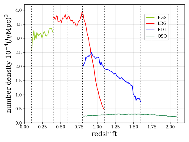
Figure 1: The comoving number density as a function of redshift for the samples used for the DESI DR1 galaxy/quasar BAO measurements. Here, we show simply the observed number of redshifts, per comoving volume element. The vertical lines represent the boundaries of the redshift bins used in this analysis, except for the QSO sample which is analyzed as a single redshift bin.

2.1 DESI DR1

The DESI Data Release 1 (DR1; [56]) dataset includes observations using the DESI instrument [57] on the Mayall Telescope at Kitt Peak, Arizona during main survey operations starting from May 14, 2021, after a period of survey validation [58], through to June 14, 2022. DESI measures the spectra of 5,000 ‘targets’ at once, using robotic positioners to place fibers in the focal plane at the celestial coordinates of the targets [59, 60]. The fibers are divided into ten ‘petals’ and carry the light to a corresponding ten climate-controlled spectrographs. The data was obtained via observations of ‘tiles’, using an observing strategy meant to prioritize completing observations in a given area of the sky [61]. Each tile represents a specific sky position and set of associated targets [36] assigned to each robotic fiber positioner. DESI dynamically divides its observing time into separate ‘bright’ time and ‘dark’ time programs, depending on observing conditions. 2744 tiles were observed in DR1 ‘dark’ time and 2275 tiles were observed in ‘bright’ time. Observations of the bright galaxy sample [62] happen in bright time while the luminous red galaxies (LRGs [63]), quasars (QSO [64]), and emission line galaxies (ELGs [65]) are observed in dark time. These data were first processed by the DESI spectroscopic pipeline [37] the morning following observations for immediate quality checks, and then in a homogeneous processing run (internally denoted as ‘iron’) to produce resulting redshift catalogs used in this paper and will be released in DR1.

2.2 DR1 Large-scale structure catalogs

The redshift and parent target catalogs were processed into large-scale structure (LSS) catalogs and two-point function measurements as described in [66, 67]. Table 2 presents the basic details on the tracer samples used in this paper; the catalogs used for the Ly-$\alpha$ BAO measurements are presented separately in [42]. In total, over 5.7 million unique redshifts are used for galaxy and quasar BAO measurements in DR1, a factor of $\sim 3$ increase compared to SDSS DR16 [4].

A key component of the LSS catalogs is the matched random sample (‘randoms’), which accounts for the survey geometry. The randoms were first produced to match the footprint of DESI target samples, as described in [36]. These were then passed through the stage of the DESI fiberassign code that determines the ‘potential assignments’ for each input random target, using all of the properties of the observed DESI DR1 tiles. The potential assignments do not require that the randoms are allocated a fiber in a full assignment run, they simply determine whether a fiber could reach their angular positions. Thus, this selection is one based on the individual position, and no fiber assignment effects are imprinted on the randoms. This procedure works to the angular scale at which the DESI fiberassign software can predict the focal plan position of targets to be observed, which is better than 1 arcsecond. It is thus far more accurate than trying to sample a pixellated angular mask. The process is detailed in [66].

These potential assignments are cut to the same combination of ‘good’ tiles and fibers as the DR1 data samples. Subsequently, veto masks are applied following the same process as applied to DR1 data described in [67]. In DR1, the randoms are normalized such that the ratio of weighted data and random counts is the same in each of the distinct regions relevant to the photometry used to target the sample. Similarly, the redshift distributions are matched between data and randoms in each region separately. For all but the QSO sample, there are two distinct photometric regions: data targeted from BASS/MzLS photometry [68] in the North Galactic Cap (NGC) and declination greater than $32.375^{\circ}$ and those targeted from DECaLS photometry (in both Galactic caps). For QSOs, the DECaLS sample is further divided into DES and non-DES regions, as the target selection [64] is different in those regions.

Supporting studies help define and correct for variations in the selection function due to the effects of imaging systematics on the input target samples [69, 23, 70] and variations in the DESI instrument’s ability to successfully measure redshifts [24, 71]. Our ability to simulate and correct for incompleteness in target assignment is presented in [72, 73, 74]. The effects of all of those issues are combined into a weight column in the data and random catalogs, meant to be used for any subsequent calculations (i.e., both for reconstruction and two-point statistics). The number density of the DR1 DESI samples varies strongly with both redshift and the number of overlapping tiles (due to assignment completeness). Thus, ‘FKP’ weights, inspired by [75], that are meant to maximize the signal to noise of clustering measurements at the BAO scale with respect to such number density variations are also included in all two-point calculations. Their calculation is fully detailed in [67].

Tracer	redshift range	$N_{\rm tracer}$	$z_{\rm eff}$	$P_{0}(k=0.14)$	$V_{\rm eff}$ (Gpc3)
BGS	$0.1-0.4$	300,017	0.30	$\sim 9.2\times 10^{3}$	1.7
LRG1	$0.4-0.6$	506,905	0.51	$\sim 8.9\times 10^{3}$	2.6
LRG2	$0.6-0.8$	771,875	0.71	$\sim 8.9\times 10^{3}$	4.0
LRG3	$0.8-1.1$	859,824	0.92	$\sim 8.4\times 10^{3}$	5.0
ELG1	$0.8-1.1$	1,016,340	0.95	$\sim 2.6\times 10^{3}$	2.0
LRG3$+$ELG1	$0.8-1.1$	1,876,164	0.93	$\sim 5.9\times 10^{3}$	6.5
ELG2	$1.1-1.6$	1,415,687	1.32	$\sim 2.9\times 10^{3}$	2.7
QSO	$0.8-2.1$	856,652	1.49	$\sim 5.0\times 10^{3}$	1.5

Table 2: Statistics for each of the DESI tracer types used for the DESI Y1 BAO measurements presented in this paper. Redshift bins are non-overlapping, except for the shot-noise dominated QSO sample and the $0.8<z<1.1$ LRG and ELG. The effective volume calculation, $V_{\rm eff}$ provides a rough estimate for the relative amount of cosmological information in each redshift bin. See text for further details on the calculation of values in this table and [67] for further details on the samples themselves.

In what follows, we provide brief details on the properties of each sample, providing further context for the statistics of each sample that are presented in Table 2. The $z_{\rm eff}$ values are calculated weighting by the square of the weighted number density of randoms (with the weights—including FKP—described above), $n_{\rm ran}(z)$:

$$z_{\rm eff}=\frac{\int zr^{2}drn^{2}_{\rm ran}(z)}{\int r^{2}drn^{2}_{\rm ran}(z)},$$ (2.1)

where $r$ is the comoving distance to the redshift $z$. These represent the redshift at which the BAO fit parameters, $\alpha_{\rm iso}$ and $\alpha_{\rm AP}$, can be converted into physical distances (see Section 8). The clustering amplitude is determined via a single parameter fit to the post-reconstruction power spectra at wavenumbers $k<0.07\ h\,\text{Mpc}^{-1}$, assuming the linear matter power spectrum given by our fiducial cosmology. The effective volume estimate is obtained in each redshift bin via

$$V_{\rm eff}=\int\left[\frac{\bar{n}_{\rm tracer}(z)P_{0}(k=0.14)}{1+\bar{n}_{\rm tracer}(z)P_{0}(k=0.14)}\right]^{2}dV(z)$$ (2.2)

where for $P_{0}(k=0.14)$ we use the values listed in Table 2, which are rounded numbers taken from the DR1 $P_{0}(k)$ measurements. The choice of $k=0.14\ h\,\text{Mpc}^{-1}$ was chosen to be most representative for BAO measurements [76]. The comoving number density as a function of redshift for each sample is shown in Figure 1.

The Bright Galaxy Sample (BGS):

The final BGS sample used for our DR1 BAO measurements comprises of $300,017$ redshifts in the interval $0.1<z<0.4$ over $7,473\deg^{2}$, with an assignment completeness of $61.6\%$ (see [67] for full details). The completed DESI BGS sample is expected to have $\sim 80\%$ assignment completeness over 14,000 deg², implying the DR1 sample contains just over 2/5 of the final DESI BGS sample. The minimum bound of $z=0.1$ is chosen to minimize any effects of bright limits ([77]) on the target sample. The maximum bound is chosen to separate the sample from the LRG sample (described next).

The nominal BGS sample is flux-limited [62] and thus has strong variation of its number density with redshift. In order to produce a more homogeneous sample a cut on the DR1 BGS sample was engineered to produce a sample of roughly constant number density of $5\times 10^{-4}\;h^{3}\,\text{Mpc}^{-3}$, for a sample with 100% fiber assignment completeness. Thus, the DR1 number density is roughly constant at $3\times 10^{-4}\;h^{3}\,\text{Mpc}^{-3}$, averaged over the DR1 footprint, as can be seen in the light green curve in Figure 1. The sample was defined using $k$-corrected $r$-band absolute magnitudes from [78, 79] and a correction for evolution that is linear in redshift (matching that used for [39]). The cuts make the sample a close match to both the LRG number density (for a complete sample) at $z=0.4$ and the clustering amplitude, as can be seen by comparing to the red curve in Figure 1 and the $P_{0}$ entries in Table 2. The density is high enough to make shot-noise a minor contribution to the BGS statistical uncertainty in the DR1 two-point measurements at BAO scales. See [67] for more details.

The Luminous Red Galaxy Sample (LRG):

The DESI DR1 LRG sample used for BAO measurements consists of $2,138,600$ good redshifts over $5,840\deg^{2}$ in the redshift interval $0.4<z<1.1$. The DR1 assignment completeness is $69.2\%$ in the Y1 sample; this is expected to increase to $90\%$ over $14,000\deg^{2}$ in the complete survey, so the DR1 LRG sample is thus approximately 30% of the full DESI LRG sample.

The lower redshift bound was chosen to separate the sample from BGS, as most low-redshift LRG targets are also BGS targets and we are able to match the densities of the two samples at $z=0.4$ (when accounting for assignment completeness). The complete LRG sample has a nearly constant number density over $0.4<z<0.8$ of $5\times 10^{-4}\;h^{3}\,\text{Mpc}^{-3}$, which becomes just over $3.5\times 10^{-4}\;h^{-3}\,\text{Mpc}^{3}$ when averaged over the DR1 area, as shown in Figure 1. The upper bound of $z<1.1$ was chosen to align with the ELG redshift bins. As for previous LRG samples, the clustering is significantly biased compared to the matter distribution, which enhances the BAO signal. The clustering amplitude is approximately constant over the entire redshift range, though there is some evolution in both the clustering amplitude and composition of the sample for $z>0.95$, as documented in [80], which causes the slight decrease in the $b\sigma_{8}$ clustering amplitude for the $0.8<z<1.1$ bin.

This sample is further split for the clustering analysis into 3 disjoint redshift ranges, $0.4<z<0.6$ (LRG1), $0.6<z<0.8$ (LRG2), and $0.8<z<1.1$ (LRG3), with this higher redshift sample overlapping the low-redshift ELG sample. The redshift binning was chosen in part to align with the SDSS BAO measurements used in [4]. The redshift bin $0.4<z<0.6$ matches one of the SDSS bins. Despite SDSS using $0.6<z<1.0$ for one of their LRG bins, the SDSS sample is dominated by galaxies with $z<0.8$ and their effective redshift is slightly lower than that of our $0.6<z<0.8$ LRG sample ($z_{\textrm{eff}}=0.7$ compared to $z_{\textrm{eff}}=0.71$). This allows us to present a direct comparison between the DESI DR1 measurements and the SDSS measurements (Section 7.6). The $0.8<z<1.1$ redshift bin is aligned with the lower redshift bin chosen for ELGs (described next), which allows a combined LRG+ELG sample to be created and used in the $0.8<z<1.1$ redshift range.

The Emission Line Galaxy Sample (ELG):

The DR1 ELG sample defined for clustering analysis in [67] comprises $2,432,022$ good redshifts in the interval $0.8<z<1.6$ over a footprint of $5,914\deg^{2}$. DESI ELGs are assigned fibers at the lowest priority of any DESI target class, and in DR1, the fiber assignment completeness is only $35.3\%$. This should increase to over 60% in the final dataset, with the footprint growing to 14,000 deg². The DR1 sample is thus less than 1/4 of the final DESI ELG sample. The clustering amplitude is the lowest of any of the DESI target classes, consistent with the general knowledge that actively star-forming galaxies are generally less clustered than passive galaxies. These lower clustering amplitudes explain why the effective volume for the $0.8<z<1.1$ ELG sample is significantly lower than the LRG sample in the same redshift bin, despite having more galaxies. One can see from Eq. 2.2 that there is a leading factor of $P_{0}^{2}$. As the DESI survey progresses, the ELG completeness will increase and thus $N_{\rm tracer}/V_{\rm tot}$ will grow larger and make the clustering amplitude less relevant to the effective volume calculation.

The sample is split into 2 disjoint redshift ranges for measuring two-point clustering: $0.8<z<1.1$ (ELG1) and $1.1<z<1.6$ (ELG2). The split at $z=1.1$ is meant to align with the maximum redshift of the LRG sample. At $z<0.8$, the ELG number density drops below that of the LRG sample, even after accounting for fiber assignment incompleteness (see [67]). Further trends with the imaging depth become severe, as shown in [23]. The upper limit of $z<1.6$ is applied as the OII emission line doublet used to secure redshifts for the ELG sample is at a longer wavelength than covered by the DESI spectrographs for $z>1.6$.

Combined LRG and ELG (LRG3$+$ELG1):

A combined LRG and ELG sample is used for $0.8<z<1.1$. Ignoring any possibility of sample variance cancellation, the optimal BAO information extracted from data in this redshift range should come from combining the two samples into one, with an appropriate weighting given the difference in clustering amplitude. The construction of this combined sample and its validation are presented in [47] and results from it are denoted ‘LRG3$+$ELG1’. Further details, including its motivation, are discussed in Section 7.5.

The Quasar Sample (QSO):

The DR1 QSO sample used for BAO measurements consists of $856,652$ good redshifts with $0.8<z<2.1$. The sample covers an area of 7,249 deg², within which the assignment completeness is $87.6\%$. The QSO assignment completeness in the completed DESI survey, which spans 14,000 deg², is expected to be greater than $99\%$. Thus, the DESI DR1 QSO sample contains just under half of the number expected for the completed survey.

The upper bound of $z<2.1$ is chosen as $z>2.1$ quasars are used as sight-lines along which Lyman-$\alpha$ forest absorption is measured and then used to obtain BAO measurements, as described in [42]. The $z>0.8$ choice is somewhat arbitrary, but aligns both with the lower bound chosen by SDSS and with the redshift bin edge adopted for LRG and ELG. The clustering amplitude of the sample is intermediate between that of the LRG and ELG samples, which makes it the most highly biased sample, given the low $\sigma_{8}(z_{\rm eff})$ at its effective redshift.

2.3 Blinding

In order to protect against confirmation bias in our DESI DR1 galaxy BAO measurements, the location of the BAO feature in our measured two-point functions for galaxies and quasars was intentionally shifted from its true values by an unknown amount by applying a blinding shift at the catalog level following the methods proposed in [81]. Full details of the specific methodology applied to DESI DR1 are presented in [54]. We summarize some basic details here. First, $w_{0},w_{a},f_{\rm NL}$ were randomly chosen from a pre-defined list of values, which were bounded to keep $\alpha_{\rm iso}$ within 3% of its fiducial value within the redshift range $0.4<z<2.1$. The primordial non-Gaussianity parameter was allowed to vary within $-15<f_{\rm NL}<15$. The choice of these bounds represented one of the final necessary choices by the DR1 cosmological analysis team prior to obtaining the first (blinded) DESI DR1 BAO measurements. The DESI redshifts were then coherently shifted based on the expected difference in redshift between the chosen $w_{0},w_{a}$ and $w_{0}=1,w_{a}=0$, at the comoving coordinates initially determined from the true redshift and the fiducial cosmology. Redshifts were also shifted based on estimates of the local density in order to blind structure growth methods. Rather than being drawn randomly, a shift in the growth rate, $f$, was chosen so that it would compensate for the expected change in the monopole of the redshift-space clustering, up to 10% of the expected change using a linear redshift-space distortions model. The $f_{\rm NL}$ shift was implemented via weights and demonstrated to have no effect on BAO measurements, beyond small random fluctuations from the effective re-weighting. Further description of the DESI DR1 blinding methodology and validation is in [54].

The cosmology of the shift was kept constant with every catalog update and never revealed. When the DR1 analyses matured to the point where all choices were frozen (see Table 14 for the tests that were first performed on the shifted data), the LSS catalogs without any shifts applied were then used for the first time, to produce two-point clustering measurements (i.e., ‘unblinded’). After the unblinded results were revealed, an error was found in the LSS catalogs related to the completeness weights that are assigned to random points. The main effect of this on BAO measurements is to re-weight the contributions from different areas of the footprint. The greatest change to the BAO fits was a $-0.7\sigma$ shift in the $\alpha_{\rm AP}$ result for LRGs with $0.4<z<0.6$. The magnitude of all other shifts were less than $0.5\sigma$, and most were less than 0.2$\sigma$. Only two pieces of the BAO analysis were updated after unblinding: 1) the final choice on the covariance matrix and 2) the use of the LRG+ELG combined sample in the $0.8<z<1.1$ redshift bin; however, both of these updates were decided/planned before unblinding.

3 Mocks

Ref	Task/Paper	Mocks
[7]	BAO Theory and Modelling Systematics	Abacus-1 cubic, CV
[45]	Extensive comparison of reconstruction methods	Abacus-1 cubic, Y5
[46]	Optimal reconstruction of BAO for DESI 2024	Abacus-2/EZmock DR1
	and the summary of the unblinding test
[47]	Constructing the LRG and ELG combined tracers	Abacus-2 DR1
[48]	Comparison between analytical and EZmock covariance matrices	EZmock DR1
[49]	Analytical covariance matrices for correlation function for DESI 2024	Abacus-2/EZmock DR1
[50]	Analytic covariance matrices of DESI 2024 power spectrum multipoles	Abacus-2/EZmock DR1
[51]	Fiducial-cosmology-dependent systematics	Abacus-2 DR1
[52]	HOD-dependent systematics for LRGs	Abacus-1 cubic, CV
[53]	HOD-dependent systematics for ELGs	Abacus-1 cubic, CV

Table 3: The table summarizes the principal set of simulations used for each supporting task/paper and the sections of this paper that make use of them. Abacus-2 and EZmock DR1 duplicate the footprint of the DESI DR1, the variation of completeness with target number density, and an approximate fiber assignment effect. The tasks that need to simulate the DESI DR1 survey realism concluded their tests with the DR1 mocks. Abacus-1 Y5 approximately traces the expected DESI Y5 footprint. The tasks that needed to test the theoretical systematics with the least level of noise utilized the cubic simulations; in this case, we used Abacus-1 cubic instead of Abacus-2, as the former was completed first and was sufficient for our analysis. CV denotes the control variate technique that was applied to the Abacus-1 cubic [82]. The CV technique allows to reduce sample variance noise from the two-point statistics by utilizing a highly correlated surrogate based on the Zeldovich approximation.

Realistic and accurate mock simulations form the backbone of our analysis. They allow us to test the limitations of our theoretical models in the presence of non-linear evolution and galaxy-halo physics. In addition, they allow us to assess our ability to mitigate imperfections in our survey caused by effects such as atmospheric conditions, foreground astrophysical systems, and instrument limitations. Building a single set of mock simulations that can be used for all these tests is not feasible because the combination of volume, resolution and number of realizations needed is beyond our current computational resources. Therefore, we build a series of DESI mock simulations focusing on the different aspects of theoretical and observational systematics. A specific set of simulations used for each task is listed in Table 3.

We built two kinds of mock simulations. The first called Abacus used the high-resolution AbacusSummit simulation suite and hence produced highly accurate non-linear structure. The second called EZmock were computationally very cheap to produce over large volumes and resulted in highly accurate linear scales but non-linear scales that were not that well controlled.

All mocks are produced at the Planck 2018 $\Lambda$CDM cosmology, specifically the mean estimates of the Planck TT,TE,EE+lowE+lensing likelihood chains: $\Omega_{c}h^{2}=0.1200$, $\Omega_{b}h^{2}=0.02237$, $\sigma_{8}=0.811355$, $n_{s}=0.9649$, $h=0.6736$, $w_{0}=-1$, and $w_{a}=0$ [31].

3.1 Abacus

AbacusSummit is a large suite of high-resolution gravity-only N-body simulations using the Abacus N-body code [55, 83]. These simulations provide us with realizations of the density field and dark matter halos in cubic boxes with a range of cosmologies. The entire suite consists of over 150 simulations at 97 different cosmologies. This study makes use of the 25 “base” boxes of the Planck 2018-$\Lambda$CDM cosmology, each of which contains $6912^{3}$ particles within a $(2h^{-1}$Gpc$)^{3}$ volume corresponding to a particle mass of $2.1\times 10^{9}$ M${}_{\odot}/h$.

The dark matter halos are identified with the CompaSO halo finder [84]. We also run a post-processing “cleaning” procedure to remove over-deblended halos in the spherical overdensity finder, and to intentionally merge physically-associated halos that have merged and then physically separated [85].

The dark matter halo catalogs are then populated with galaxies using an extended halo occupation distribution (HOD) model with the AbacusHOD code [86]. These Abacus mocks were produced in two generations called Abacus-1 and Abacus-2. The main difference between the two comes from the fact that they were produced at different times to be able to make early progress on testing the analysis pipeline while we collect more data and improve our model of the survey and instrument. The Abacus-1 used very early version of the DESI early data release (DESI-EDR)[39] to find the best fit halo occupation distribution model whereas Abacus-2 used the final DESI-EDR after correcting for all the systematics and including a detailed model for DESI focal plane effects.

Abacus-1

These mocks were produced by fitting the galaxy two-point correlation function averaged in angular bins at small scales using Abacus halos and a flexible halo occupation distribution model (HOD) [87] to populate these halos with galaxies. We found best-fit HOD parameters at each available snapshot between redshift of 0 to 2 in the AbacusSummit suite. The details of HOD models used are described in [88]. We note that satellite galaxies were distributed using NFW profiles fit to the density profile of each halo in the simulation. For the QSO mocks we also included an additional velocity dispersion to account for the significant QSO redshift errors. Each tracer at each redshift is populated over all 25 base boxes, giving a total volume of 200$h^{-3}$Gpc³.

Abacus-2

The HOD parameters are tuned to the final DESI EDR redshift-space two-point correlation function measurements. We refer the readers to [80, 89, 90] for the exact HOD models and calibration. The final cubic mocks consists of BGS samples at $z=0.1,0.2,0.4$, LRG samples at $z=0.5,0.8,1.1$, ELG samples at $z=0.95,1.1,1.325$, and QSO samples at $z=1.1,1.4,1.7$. Each tracer at each redshift is populated over all 25 base boxes, for a total volume of 200$h^{-3}$Gpc³. We also provide Zeldovich control variates (ZCV) mock simulations with suppressed sample variance for all AbacusSummit realizations (see [82] for description of the technique).

3.2 EZmock 

In order to generate large simulation volumes for covariance matrices and pipeline validations, we use the EZmock code [91] which can be calibrated to accurately reproduce the two- and three-pt clustering on the scales relevant for this analysis without the cost of a full N-body simulation. It has been widely used in eBOSS [92] and DESI [93].

The method comprises two steps: constructing a dark matter density field and populating galaxy catalogs. The dark matter density field is based on the the Zel’dovich approximation [94]. To populate the resulting density field with galaxies, EZmock uses an effective bias model to account for non-linear evolution and galaxy bias. The latest description of the effective bias model can be found in [92]. We produced two generations of DESI EZmock by fitting the two-point clustering of Abacus-1 and Abacus-2  in order to give equivalent covariance matrices. We produced 1000 realizations of each generation of EZmock with a box side of 2$h^{-1}$Gpc. These provide the covariance matrix for equivalent 2$h^{-1}$Gpc Abacus mocks. We also produced 1000 realizations of each generation of EZmock with a box side of 6$h^{-1}$Gpc in order to fit the volume occupied by the DESI DR1 data without any repetition of structure to validate our covariance matrices for the full survey volume.

3.3 Simulations of DR1

Both the Abacus-2  and 6$h^{-1}$Gpc EZmock have been used to simulate the DESI DR1 LSS dataset [95]. A brief outline of the steps to create such mocks is as follows: For both, the first step is to transform the box coordinates to angular sky coordinates and redshifts. Then, the data are sub-sampled as a function of redshift such that the total projected density matches that of the given target sample and the $n(z)$ (after accounting for redshift failures) matches that of the observed DR1 sample [67]. This provides a simulated DESI target sample. The simulated target sample is then cut so that it covers the same sky area as the DESI target samples. Then, matching the process applied to randoms described in Section 2.2, it is passed through the stage of the DESI fiberassign code that determines the ‘potential assignments’ for each simulated target, using all of the properties of the observed DESI DR1 tiles. These potential assignments are cut to the same combination of ‘good’ tiles and fibers as the DR1 data samples. Subsequently, veto masks are applied following the same process as applied to DR1 data described in [96].

The process described above reproduces the small-scale structure of the DESI DR1 footprint, but does not impart any incompleteness within it. For the Abacus-2, mock LSS catalogs (hereafter mocks) were produced with three variations in the fiber assignment completeness. These are:

• The ‘complete’ mocks that have no assignment incompleteness added and thus can be used as a baseline comparison for understanding the effect of the incompleteness.

• The ‘altmtl’ mocks that represent our most realistic simulations of the DR1 data. They apply the process described in [72] to apply the DESI fiberassign code to tiles in the same ordering and cadence in a feedback loop to the target list as occurred for the observed data. The process was demonstrated to perfectly reproduce DESI fiber assignment on real DESI targets, with no approximations.

• The ‘fast-fiberassign’ mocks that emulate the fiber assignment process by sampling from the average targeting probability of the galaxies multiple times, learned from the data as a function of number of overlapping tiles and local (angular) clustering. The final sample is obtained by recombining the multiple realisations in such a way that deliberately creates a small-scale exclusion effect, which approximately reproduces the fiber-collisions pairwise incompleteness. The process is much faster than the altmtl and is described and validated in [73].

The computation time required for the altmtl mocks prohibits it from being run on all 1000 EZmocks. Thus, we apply only the fast-fiberassign process to the EZmocks.

All flavors of mocks go through the process of assigning redshifts and weights to randoms in the same way as for the real data samples and are normalized within the same regions, etc (e.g., all integral constraints effects, e.g., described in [97], are the same between data and mock LSS catalogs) following the prescription in [67]. More details about the creation and validation of the different mock flavours can be found in [95].

4 Methods

This section summarizes the various methods used in the BAO analyses that follow. We refer the reader to the referenced supporting papers for more detail and validations.

4.1 Two-point function codes

The BAO measurements derive from the two-point clustering statistics of the data, the correlation function in configuration-space and the power spectrum in Fourier space. The techniques for computing these are now well established. We use the Landy-Szalay estimator [98] for the correlation functions (modified as in [99] for the reconstructed data) and an FKP based estimator ([100, 101]) for the power spectrum. A more detailed discussion of our particular implementations can be found in [67]. The specific codes are pycorr for correlation functions and pypower for power spectra. We compress the angular dependence (to the line of sight) into Legendre multipoles; our analyses rely on the $\ell=0$ (monopole) and $\ell=2$ (quadrupole) components. The galaxies are weighted by terms to account for the selection function and to optimally measure two-point statistics (FKP weights), both summarized in Section 2 and fully defined in [96], unless otherwise noted.

Since the clustering measurements are consistent for both Galactic caps, we combine these measurements when constructing our data vectors. In configuration-space, the combination is performed by summing the pair counts computed in each region independently. Similarly, the power spectrum estimates are obtained for each Galactic cap and the measurements are then combined by averaging the two power spectra, weighting by their respective normalizations [67]. The number of randoms used is more than 50$\times$ the size of the data for all correlation functions measurements and more than 100$\times$ for all power spectra.

The DESI fiber assignment imprints structure into the two-point statistics, especially on small scales. This can be mitigated very effectively by removing small-angle/small-separation pairs in the two-point statistics [74]. While such an approach is necessary for analyses that use the full shape of the two-point function, we expect these fiber assignment issues to have no measurable impact on our extraction of the BAO distance scales. This is both a result of the fact that the BAO feature is at large scales, and that we marginalize out the overall shape of the two-point function in our analysis. We validate this with mocks with and without fiber assignment and find no impact at greater than 2$\sigma$ significance (Section 5.3). Note that this does not include accounting for the overall completeness, which we do in our galaxy weights. Given this insensitivity, we do not include any additional corrections for fiber assignment in our analysis.

4.2 Density-field reconstruction

Density-field reconstruction [12] is now a well-established element of galaxy BAO analyses, as it robustly eliminates biases due to the nonlinear evolution of the density field and improves the statistical precision of the BAO method. Beyond the standard reconstruction method proposed in [12], which has been widely applied to observational datasets [99, 19, 102, 103, 104, 105], there are several improved reconstruction algorithms that have been proposed in the literature [106, 107, 108]. Although these methods have significant promise for reconstructing the linear density field at small scales at the very low shot noise regime, the improvements in the BAO distance measurements are marginal at the galaxy number densities of DESI DR1. Considering this and the robustness and simplicity of the original method, we restrict ourselves to using it for this work, with the modifications described below.

• One of the main differences from previous applications of reconstruction in SDSS is the use of the RecSym convention [17]. RecSym shifts the tracers and randoms from the LSS catalogs in the same way using the redshift-space displacement, preserving RSD in the post-reconstruction clustering. The RecIso convention [99] used in BOSS and eBOSS approximately removes RSD, resulting in more isotropic clustering post-reconstruction. We adopt the RecSym convention as our baseline since it is the choice that fully removes the nonlinear damping and shift of the BAO due to large-scale modes [7] and avoids artefacts in the correlation function on small scales. However, [46] shows that the DESI BAO constraints in practice are rather insensitive to this choice (a similar conclusion was found in [109]).

• We tested the sensitivity of the reconstruction method to the choice of scale that is used to smooth the density field. Using the blinded DESI data and mocks that match the expected clustering properties of DESI DR1, we determined the optimal smoothing scale to be used when reconstructing each DESI target sample, as described in [46] and presented in Table 4.

Our reconstruction uses pyrecon, a Python package developed by the DESI collaboration. This comprehensive toolkit offers a diverse range of reconstruction algorithms and accommodates various conventions, and provides the flexibility to process periodic-box simulations or survey data with non-uniform geometries. In terms of the numerical implementation of the reconstruction method, we adopt an efficient algorithm based on iterative Fast Fourier Transforms introduced in [110] as our baseline, which we find highly consistent with the output from MultiGrid. The iterative Fast Fourier Transform we adopt is different from the method in eBOSS. In eBOSS [111, 4], the method iteratively updates the locations of the galaxy and random particles, which we will denote as IFFTP, while the method we adopt for DESI DR1 iteratively updates the density of given meshes (hereafter, simply IFFT). This is the first time that the IFFT method (the latter) has been implemented in data analysis. An extensive comparison of reconstruction algorithms in the context of DESI is presented in [45].

Tracer	Redshift range	Linear bias $b$	Growth rate $f$	Smoothing scale $\Sigma_{\rm sm}$
BGS	0.1–0.4	1.5	0.68	$15\,h^{-1}{\rm Mpc}$
LRGs	0.4–1.1	2.0	0.83	$15\,h^{-1}{\rm Mpc}$
ELGs	0.8–1.6	1.2	0.90	$15\,h^{-1}{\rm Mpc}$
QSO	0.8–2.1	2.1	0.93	$30\,h^{-1}{\rm Mpc}$

Table 4: Redshift range, tracer linear bias, growth rate of structure, and smoothing scale assumed when reconstructing each DESI target sample. The smoothing scale was chosen after testing different values for each tracer, as detailed in [46].

Table 4 summarizes the different hyperparameters that we calibrated when reconstructing the DESI DR1 samples. The catalogs were reconstructed across the entire redshift range of each tracer simultaneously, assuming a value of the growth rate of structure determined by our fiducial cosmology and the effective redshift of each sample.

4.3 Defining the clustering model

We next describe the BAO fitting method used in the galaxy DR1 analysis. We design this method to fully isolate the BAO feature within the broader two-point clustering measurements by combining a physically motivated theory model from quasi-linear theory and a parameterised model to marginalise over non-linearities that may otherwise affect our measurements of the BAO scale. The design of our method is based on detailed past investigations, starting from the original works of [12] with improvements through the eras of BOSS and eBOSS [19, 112, 113, 114, 20, 115, 105, 111]. Although these references have demonstrated the BAO fitting methodology to be robust at a level beyond that required for these previous surveys, there remained some inconsistencies in the modelling of the power spectrum and correlation function, and some arbitrariness in the choice of free parameters dependent upon the specific configuration and signal to noise of the measurements. As such, the modelling choices motivated or adopted in previous works have all been revisited in [7] to ensure a robust fit for the DESI DR1 results, using a method based on the allowed physical degrees of freedom that can also be consistently used for future surveys without significant modification. We have taken particular care to develop a more consistent modelling in Fourier and configuration-space, and to better motivate (or remove the need for) different modelling choices. Where such choices remain, we have quantified their systematic differences in the BAO constraints (see Section 5). In this subsection, we provide an overview of the official DESI galaxy BAO modelling prescription and summarise those changes.

4.3.1 Fourier-space fitting framework

Our generic model for the galaxy power spectrum as a function of scale $k$ and (cosine) angle $\mu$ in the “true” cosmology can be written as

$$P(k,\mu)=\mathcal{B}(k,\mu)P_{\rm nw}(k)+\mathcal{C}(k,\mu)P_{\rm w}(k)+\mathcal{D}(k)\,,$$ (4.1)

where $P_{\rm nw}(k)$ and $P_{\rm w}(k)$ denote the smooth (no-wiggle) and BAO (wiggle) components of the linear power spectrum, respectively, which are obtained using the peak average method from [116]. The linear matter power spectrum template is predicted from class using our fiducial cosmology (see Section 1). Generally, the term $C(k,\mu)P_{\rm w}(k)$ encompasses the BAO component we are interested in, damped by non-linear galaxy motions [12]; while $\mathcal{B}(k,\mu)P_{\rm nw}(k)$ uses quasi-linear theory to model the smooth component of the galaxy clustering, and $\mathcal{D}(k)$ is our parametric model to account for additional non-linearities and observational effects. This model generally matches that used in previous BAO analyses [19, 112, 103, 104], but the exact forms of each component differ and so will be discussed later in this section.

In order to make contact with the apparent size of the BAO seen in the fiducial cosmology, $C(k,\mu)P_{\rm w}(k)$ is evaluated at Eq. 1.1,

$$k^{\prime}=\frac{\alpha_{\text{AP}}^{1/3}}{\alpha_{\text{iso}}}\left[1+\mu^{2}_{\rm obs}\left(\frac{1}{\alpha_{\text{AP}}^{2}}-1\right)\right]^{1/2}k_{\rm obs}$$ (4.2)

and

$$\mu^{\prime}=\frac{\mu_{\rm obs}}{\alpha_{\text{AP}}}\left[1+\mu_{\rm obs}^{2}\left(\frac{1}{\alpha_{\text{AP}}^{2}}-1\right)\right]^{-1/2},$$ (4.3)

where the subscript ‘obs’ is used to distinguish between observed coordinates and measurements (assuming a fiducial cosmology) and those in the (unknown, but to be constrained) true cosmology. Note that this transformation is not just a coordinate transformation between the true and fiducial cosmologies but also includes a rescaling of the BAO template from the template cosmology, reflecting that what is measured is the apparent size of the BAO relative to the template sound horizon. The true, fiducial and template cosmologies need not be the same ([51], see also Section 5.4), but the latter two are usually equated for simplicity. The rescaling in Eqs. 4.2 and 4.3 in principle should not apply to the non-BAO parts of the power spectrum. In order to prevent accidentally using broadband information in the smooth component in the DESI DR1 analysis, we hence evaluate the smooth components directly at the observed coordinates, without dilation. The model for the power spectrum multipoles is thus

$$P_{\ell,\rm obs}(k_{\rm obs})=\frac{2\ell+1}{2}\int_{-1}^{1} d\mu_{\rm obs}\ \mathcal{L}_{\ell}(\mu_{\rm obs})\big{[}\mathcal{B}(k_{\rm obs},\mu_{\rm obs})P_{\rm nw,obs}(k_{\rm obs})$$

$$+\mathcal{C}(k^{\prime}(k_{\rm obs},\mu_{\rm obs}),\mu^{\prime}(k_{\rm obs},\mu_{\rm obs}))P_{\rm w}(k^{\prime}(k_{\rm obs},\mu_{\rm obs}))\big{]}+\mathcal{D}_{\ell}(k_{\rm obs}).$$ (4.4)

This is similar to that used in [115], but with the key difference that the term $\mathcal{B}(k,\mu)P_{\rm nw}(k)$ is not dilated. As a final technicality, we note that our rescaling is applied to the entire BAO component; strictly speaking the prefactor $C(k,\mu)$ is not subject to the exact same rescaling as $P_{\rm w}$, but the differences will be degenerate with the free parameters within $C(k,\mu)$ itself. We will now describe each remaining model component in turn.

Following previous BAO studies [117, 115], we adopt the following parametric form for $\mathcal{B}(k,\mu)$:

$$\mathcal{B}(k,\mu)=\left(b_{1}+f\mu^{2}[1-s(k)]\right)^{2}F_{\rm fog}\,,$$ (4.5)

where $F_{\rm fog}=\left(1+\frac{1}{2}k^{2}\mu^{2}\Sigma_{s}^{2}\right)^{-2}$ accounts for the ‘Fingers of God’ effect due to halo virialization [118, 119] via a single free smoothing scale $\Sigma_{s}$. The term $\left(b_{1}+f\mu^{2}[1-s(k)]\right)^{2}$ is a generalised form of the Kaiser factor [120] that also accounts for impact of reconstruction; here $b_{1}$ is the linear galaxy bias for the particular sample we are fitting, while $f$ is the linear growth rate of large scale structure, both of which are free parameters in our model. For pre-reconstruction and the RecSym convention, $s(k)=0$, while for RecIso, $s(k)=\exp\left[-(k\Sigma_{\rm sm})^{2}/2\right]$ and $\Sigma_{\rm sm}$ is the smoothing scale we applied to the density field during the reconstruction process.

The function $\mathcal{C}(k,\mu)$ captures the anisotropic non-linear damping of the BAO feature on top of linear theory. Similarly to the smooth component above we have that it takes the form ([7], see also ref. [121])

$$\mathcal{C}(k,\mu)=\left(b_{1}+f\mu^{2}[1-s(k)]\right)^{2}\exp\left[-\frac{1}{2}k^{2}\biggl{(}\mu^{2}\Sigma_{||}^{2}+(1-\mu^{2})\Sigma^{2}_{\perp}\biggl{)}\right]$$ (4.6)

where $\Sigma_{||}$ and $\Sigma_{\perp}$ model the damping for modes along and perpendicular to the line of sight. The FoG factor in Equation 4.5 is dropped here due to its high correlation in fits with the damping parameters [7]. In RecIso two caveats apply: (a) the smoothing kernel $s(k)$ is always evaluated in the observed coordinates $k_{\rm obs}$, since it is defined in the fiducial cosmology and (b) the simple exponential form here is approximate and only holds on small scales where the contribution from the randoms is negligible. At intermediate scales the damping due to long-wavelength modes takes on a more complex form since the randoms and galaxies are displaced by different amounts, which is one of the reasons we choose RecSym as our default convention, as it is the unique choice that removes the nonlinear damping and shift due to long-wavelength modes. However, we note that past BAO measurements have often empirically employed the exponential form along with the prefactor in Eq. 4.5 for RecIso, and we will continue to do so here in tests involving this scheme.

Finally, the $\mathcal{D}(k)$ factor captures any deviation from linear theory in the broadband shape of the power spectrum multipoles. Past analyses have used a polynomial form for this [19, 112, 115, 20, 105, 111], although a single exact equation cannot be provided here for comparison due to different studies using polynomial equations with different numbers of terms. To improve on this, in DESI DR1 we instead parameterize it using a spline basis with bases separated by a single user defined scale $\Delta$,

$$\mathcal{D}_{\ell}(k)=\sum_{n=-1}^{n_{\mathrm{max}}}a_{\ell,n}W_{3}\left(\frac{k}{\Delta}-n\right)\,$$ (4.7)

where $W_{3}$ is a piecewise cubic spline kernel [122, 123] and $n_{\mathrm{max}}$ sets the number of broadband terms we consider. A suitable $\Delta$ is chosen under the premise that the spline basis is able to match the broadband shape of the power spectrum without reproducing the BAO wiggles themselves. This sets a limit on the choice of $\Delta$ to be larger than half the BAO wavelength ($\pi/r_{\mathrm{d}}$ where $r_{\mathrm{d}}$ is the sound-horizon at the baryon-drag epoch). We hence use twice this minimum value, $\Delta=2\pi/r_{\mathrm{d}}\simeq 0.06h\,{\rm Mpc^{-1}}$. The number of broadband terms $n_{\mathrm{max}}=7$ for our default fitting procedure then arises from considering how many spline terms of width $\Delta$ are required to fully span the $0.02h\,{\rm Mpc^{-1}}<k<0.30h\,{\rm Mpc^{-1}}$ range of our power spectrum measurements, i.e., there is no need to specify a choice for $n_{\mathrm{max}}$. Unlike previous analyses, our new method hence provides a more physically motivated and less arbitrary broadband model.

Finally, the model multipoles need to be convolved by the data window function. This can be accomplished via matrix multiplication $\tilde{P}_{\tilde{\ell}}(\tilde{k}_{i})=\sum_{j}W_{\tilde{\ell}\ell}(\tilde{k}_{i},k_{j})P_{\ell}(k_{j})$ which can be compared directly to the data vector. This follows previous approaches [124, 125]. To ensure accuracy in this convolution, the unconvolved model is evaluated at $k$-points within $0.001h\,{\rm Mpc^{-1}}<k<0.35h\,{\rm Mpc^{-1}}$ and separated by $\Delta k=0.001h\,{\rm Mpc^{-1}}$. The computational binning is thus five times finer than the $k$-bins of the data vector $\tilde{k}$, while covering a larger $k$-range. For the theory input to $P_{\ell}(k_{j})$ we include angular dependence up to the hexadecapole. This is because power from these higher order moments can still ‘leak’ into the observed multipoles (monopole and quadrupole, or monopole only in case of 1D fits) due to the convolution with the window function $W_{\tilde{\ell}\ell}(\tilde{k},k)$ — in principle higher order multipoles can also enter but their contributions are negligible on the scales we fit.

In summary, our model for the BAO can be evaluated for comparison to data using Eq. 4.4, with the functional forms and free model parameters described in Eqs. 4.5- 4.7. Fitting for these free parameters proceeds as detailed in Section 4.4.

4.3.2 Configuration-space framework

Our approach for modelling the correlation function very closely follows that for the power spectrum, more so than in previous works [112, 20]. We start with the power spectrum multipoles in fiducial coordinates obtained from Eq. 4.4, before the window function convolution, and without the $\mathcal{D}_{\ell}(k)$ terms. These multipoles are Hankel-transformed to configuration-space to yield the correlation function multipoles in the same coordinates

$$\xi_{\ell,\rm obs}(s)=i^{\ell}\int_{0}^{\infty}\frac{dk\ k^{2}}{2\pi^{2}}j_{\ell}(ks)P_{\ell,\rm obs}(k)\,,$$ (4.8)

where $j_{\ell}$ are the spherical Bessel functions. As a direct transform of the power spectrum, the correlation function model hence also contains the same BAO dilation parameters, BAO and Fingers of God damping parameters, linear galaxy bias and growth of structure, with the same physical interpretation. We evaluate our theory model in narrow bins of $\Delta s=1h^{-1}\,{\rm Mpc}$. We match our wider $\Delta s=4h^{-1}\,{\rm Mpc}$ measurement binning by averaging the theory, weighted by the number of random - random pair counts in each fine $\Delta s=1h^{-1}\,{\rm Mpc}$ bin.

For the remaining broadband modelling, we Hankel-transform the same spline basis functions $\mathcal{D_{\ell}}(k)$ as used for the power spectrum. However, all of these except for the $n=[0,1]$ terms of  Eq. 4.7 in the quadrupole quickly go to zero on large scales, and so do not need to be included given the choice of fitting scales we use in configuration-space model. These two terms are explicitly evaluated as

$$\Delta^{3}B_{2,n}(s\Delta)=i^{2}\int\frac{dk\ k^{2}}{2\pi^{2}}\ \,W_{3}\left(\frac{k}{\Delta}-n\right)\ j_{2}(ks)$$ (4.9)

for $n=0$ and 1. However, we also introduce two additional nuisance terms for each multipole to account for the potential impact of uncontrolled large-scale data systematics. Such effects can be confined to $k<k_{\rm min}$ in Fourier space and removed by truncating the range of scales used in our fit to the power spectrum data. However, in the configuration-space, these are modelled using

$$\tilde{\mathcal{D}}_{\ell}(s)={b}_{\ell,0}+{b}_{\ell,2}\left(\frac{sk_{\rm min}}{2\pi}\right)^{2}.$$ (4.10)

with $k_{\mathrm{min}}=0.02\ h\,\text{Mpc}^{-1}$. In summary, the configuration-space broadband terms comprise of:

$$\tilde{\mathcal{D}}_{0}(s) =b_{0,0}+b_{0,2}\left(\frac{sk_{\rm min}}{2\pi}\right)^{2}\,,$$ (4.11)

$$\tilde{\mathcal{D}}_{2}(s) =b_{2,0}+b_{2,2}\left(\frac{sk_{\rm min}}{2\pi}\right)^{2}+\Delta^{3}\left(a_{2,0}B_{2,0}(s\Delta)+a_{2,1}B_{2,1}(s\Delta)\right)$$ (4.12)

with $B_{2,0}(s\Delta)$ and $B_{2,1}(s\Delta)$ given by Eq. 4.9.

4.3.3 Polynomial-based broadband modeling

For select comparisons with previous BOSS/eBOSS literature, we will occasionally compare our DESI results using the default spline-based broadband model with a more traditional polynomial-based model. In Fourier space, this latter choice consists of writing $\mathcal{D}_{\ell}(k)=\sum_{n=-1}^{3}a_{\ell,n}k^{n}$. In configuration-space, this is $\tilde{\mathcal{D}}_{\ell}(s)=\sum_{n=0}^{2}\tilde{a}_{\ell,n}s^{-n}$. Note that even when using this polynomial option, we still include all the other improvements made in DESI 2024, except for the different broadband functions.

4.3.4 Main differences between DESI 2024 and previous BAO modelling

Here we provide a summary of the most important differences in our DESI 2024 BAO modeling compared to the previous methods used in BOSS and eBOSS [19, 112, 20, 115, 105, 111]. This covers only those differences we deem most relevant to the interpretation of our fitting results, or that contribute to our systematic error budget. A more comprehensive list including more minor changes can be found in [7]. Overall, we find that the sum total of the differences between our new methodology and that used in BOSS/eBOSS result in only a small systematic error, far below DESI DR1precision (See Section 5.1).

1. As described in Section 4.2, our BAO fitting model is calibrated for RecSym as a fiducial reconstruction procedure. BOSS/eBOSS used the RecIso convention, with caveats as described around Eq. 4.6. The RecSym form of reconstruction is more physically motivated, and leads to a much simpler form for the BAO damping. We note however that [46] demonstrate consistent constraints on DESI DR1 blinded data even when using RecIso.

2. BOSS/eBOSS most frequently used a polynomial-based broadband (Section 4.3.3, although with varying numbers of free-parameters between different studies). We prefer to use a spline-based model to marginalise over non-linear physics in the broadband as this leads to a less arbitrary choice in the number of free parameters, and greater consistency between the power spectrum and correlation function. Though we believe our new approach to be better, we detect small differences between the two approaches for ${\alpha_{\rm AP}}$ which we adopt into our systematic error budget.

3. When including FoG damping, BOSS/eBOSS analyses usually applied this equally to both the wiggle and no-wiggle components (i.e., [20, 115]). Ref. [7] (figure 12 therein) demonstrated that this introduces a degeneracy between the FoG and BAO damping parameters. We hence include FoG damping only in the no-wiggle component, which removes this degeneracy. The freedom we give to the two BAO damping parameters is sufficient to account for non-linearities that can move them away from their theoretical values, and we find no systematic differences between the two methods.

4. We treat the correlation function model purely as the Hankel transform of the power spectrum, applying all our modelling choices and BAO dilation to the power spectrum first. The exception is the broadband terms, which are applied separately to the power spectrum and correlation function; nonetheless, the form of these for the correlation function is still based purely on what one obtains from Hankel transforming the spline-based broadband model for the power spectrum. This is an improvement in the consistency of the modelling compared to [112, 20]. Nonetheless, we tested both methods on our mocks and data and conservatively adopt the small difference in ${\alpha_{\rm AP}}$ into our systematic error budget.

4.4 Fitting the clustering data

The galaxy DESI 2024 BAO results in this work are obtained using desilike, a python package that provides a common framework for writing DESI likelihoods. The BAO theory and likelihood is implemented in JAX [126]. Even though gradient-based sampling methods were implemented, we found that with analytic marginalization over broadband parameters that leaves a few sampled parameters, and using Jax just-in-time compilation and parallelization capabilities, the ensemble sampler emcee [127] provided well-sampled posterior estimates in a just a few minutes. In addition to MCMC sampling, we also perform posterior profiling using desilike’s wrapping of Minuit [128].

During the course of this work, we also used/developed a fully independent galaxy BAO fitting pipeline (Barry [129]), for some of the supporting papers and with which we tested the consistency of our results prior to unblinding. This latter code was also used to demonstrate that our results are independent of the choice of MCMC/Nested sampling algorithm used [7]. We adopt desilike as our official pipeline, owing to the greater computational speed offered by its JAX implementation, and its better integration within the wider set of DESI pipelines used for producing the clustering measurements (Section 4.1 [67]), and for the cosmological interpretation of our BAO constraints [43].

For our default fitting, we adopt Gaussian priors on the BAO and Finger-of-God damping parameters and flat priors for all other model parameters. We parameterize the linear RSD though a parameter $d\beta=f/f_{\mathrm{fid}}$ where $f_{\mathrm{fid}}$ is the fiducial value for the growth rate at the effective redshift of the sample. Furthermore, $a_{0,n},a_{2,n}$ are scaled by the amplitude of the fiducial no-wiggle power spectrum at the pivot points $k_{p}=n\Delta$ before injecting them into Eq. 4.7. All of these are simple rescalings of the parameters described in Section 4.4 to improve the convergence of the fitting.

All our priors are listed in Table 5. The choices for the Gaussian priors, particularly their central values, were informed by a combination of theoretical calculations, measurements of the cross-correlation between the initial and post-reconstruction density fields in Abacus-2 DR1 simulations, and by running fits to mock catalogs for each tracer. By fitting the average over many mocks, we ensured that the signal-to-noise ratio is large enough to let the damping parameters vary freely during the fit. The resulting central values for the priors are given in Table 6. In Section 7, we show that the recovered BAO parameters from fits to DESI DR1 are largely insensitive to this choice of priors.

We perform two-dimensional fits to monopole and quadrupole data for LRGs and ELG2. For the BGS, ELG1, and QSO samples, we perform only one-dimensional fits to the monopole due to their relatively noisier clustering measurements based on the unblinding tests detailed in Table 14. In these 1-D cases, ${\alpha_{\rm AP}}$ and $d\beta$ are set to unity.

Parameter	$P(k)$ prior	$\xi(r)$ prior	Description
${\alpha_{\rm iso}}$	[0.8, 1.2]	[0.8, 1.2]	Isotropic BAO dilation.
${\alpha_{\rm AP}}^{*}$	[0.8, 1.2]	[0.8, 1.2]	Anisotropic (AP) BAO dilation.
$\Sigma{\perp}$	$\mathcal{N}(\Sigma^{\mathrm{fid}}_{\perp},1.0)$	$\mathcal{N}(\Sigma^{\mathrm{fid}}_{\perp},1.0)$	Transverse BAO damping [$h^{-1}\,{\rm Mpc}$]
$\Sigma{\parallel}$	$\mathcal{N}(\Sigma^{\mathrm{fid}}_{\parallel},2.0)$	$\mathcal{N}(\Sigma^{\mathrm{fid}}_{\parallel},2.0)$	Line-of-sight BAO damping [$h^{-1}\,{\rm Mpc}$]
$\Sigma_{s}$	$\mathcal{N}(2.0,2.0)$	$\mathcal{N}(2.0,2.0)$	Finger of God damping [$h^{-1}\,{\rm Mpc}$]
$b_{1}$	$[0.2,4]$	$[0.2,4]$	Linear galaxy bias
$d\beta^{*}$	$[0.7,1.3]$	$[0.7,1.3]$	Linear RSD parameter
$a_{0,n}$	$\mathcal{N}(0,10^{4})$	N/A	Spline parameters for the monopole
$a_{2,n}^{*}$	$\mathcal{N}(0,10^{4})$	$\mathcal{N}(0,10^{4})$	Spline parameters for the quadrupole
$b_{0,n}$	N/A	[$-\infty,\infty$]	Unknown large scale systematics
$b_{2,n}^{*}$	N/A	[$-\infty,\infty$]	Unknown large scale systematics
Fitting range	[0.02, 0.3]$\ h\,\text{Mpc}^{-1}$	[48, 152]$\ h^{-1}\text{Mpc}$	Measurement bin edges
Data binning	$0.005\ h\,\text{Mpc}^{-1}$	$4\ h^{-1}\text{Mpc}$	Measurement bin width

Table 5: The free parameters and their priors for Fourier-space (FS) and configuration-space analyses. $\mathcal{N}(\mu,\sigma)$ refers to a normal distribution of mean $\mu$ and standard deviation $\sigma$, $[x_{1},x_{2}]$ to a flat distribution between $x_{1}$ and $x_{2}$ inclusive. For faster fitting and convergence, we re-parameterise our linear RSD parameter using $d\beta=f/f_{\mathrm{fid}}$, where $f_{\mathrm{fid}}$ is fiducial growth rate. $a_{0,n},a_{2,n}$ are also scaled by the amplitude of the fiducial no-wiggle power spectrum at the pivot points $k_{p}=n\Delta$ before injecting them into Eq. 4.7. Parameters with superscript ‘$*$’ are fixed to the following values when only a 1D fit is performed: ${\alpha_{\rm AP}}=1$, $d\beta=1$, $a_{2,n}=0$, $b_{2,n}=0$. The central values of the Gaussian BAO damping parameters, denoted by superscript ‘fid’ vary between tracers and so are provided separately in Table 6. $\Sigma{\perp}$, $\Sigma_{\parallel}$ and $\Sigma_{s}$ are additionally bounded between $[0,20]$. The total number of free parameters for our 1D and 2D fits are 15 and 25 respectively for $P(k)$; and 7 and 13 respectively for $\xi(r)$. The corresponding numbers of degrees-of-freedom for our 1D and 2D fits are 41 and 87 for $P(k)$; and 19 and 39 for $\xi(r)$.

Tracer	Redshift range	$\Sigma^{\mathrm{fid}}_{\perp}[h^{-1}\,{\rm Mpc}]$		$\Sigma^{\mathrm{fid}}_{\parallel}[h^{-1}\,{\rm Mpc}]$
		Pre-recon	Post-recon	Pre-recon	Post-recon
BGS	0.1 - 0.4	6.5	3.0	10.0	8.0
LRG	0.4 - 0.6	4.5	3.0	9.0	6.0
LRG	0.6 - 0.8	4.5	3.0	9.0	6.0
LRG	0.8 - 1.1	4.5	3.0	9.0	6.0
ELG	0.8 - 1.1	4.5	3.0	8.5	6.0
ELG	1.1 - 1.6	4.5	3.0	8.5	6.0
QSO	0.8 - 2.1	3.5	3.0	9.0	6.0

Table 6: The central values of the BAO damping parameters used for our default Gaussian priors (see Table 5) when fitting each of the DESI DR1 tracers. These are obtained from a combination of theoretical calculations, measurements of the cross-correlation between the initial and post-reconstruction density fields in Abacus-2 DR1 mocks, and by running fits to data vectors averaged over many realizations of these mocks for each tracer.

For Fourier-space fits, the theory model always includes all three multipoles for the product with the window matrix, but the broadband terms for the multipoles that are not fitted (e.g. quadrupole and hexadecapole for 1-D fits) are set to $0$ as they are mostly unconstrained.

In the rest of this work we mainly report on the BAO scaling parameters $\alpha_{\text{iso}}$ and $\alpha_{\text{AP}}$, but in doing so are fully marginalizing over the other parameters of our model, including the correlation function/power spectrum broadband parameters, the galaxy bias, and the damping parameters.

4.5 Covariance Matrices

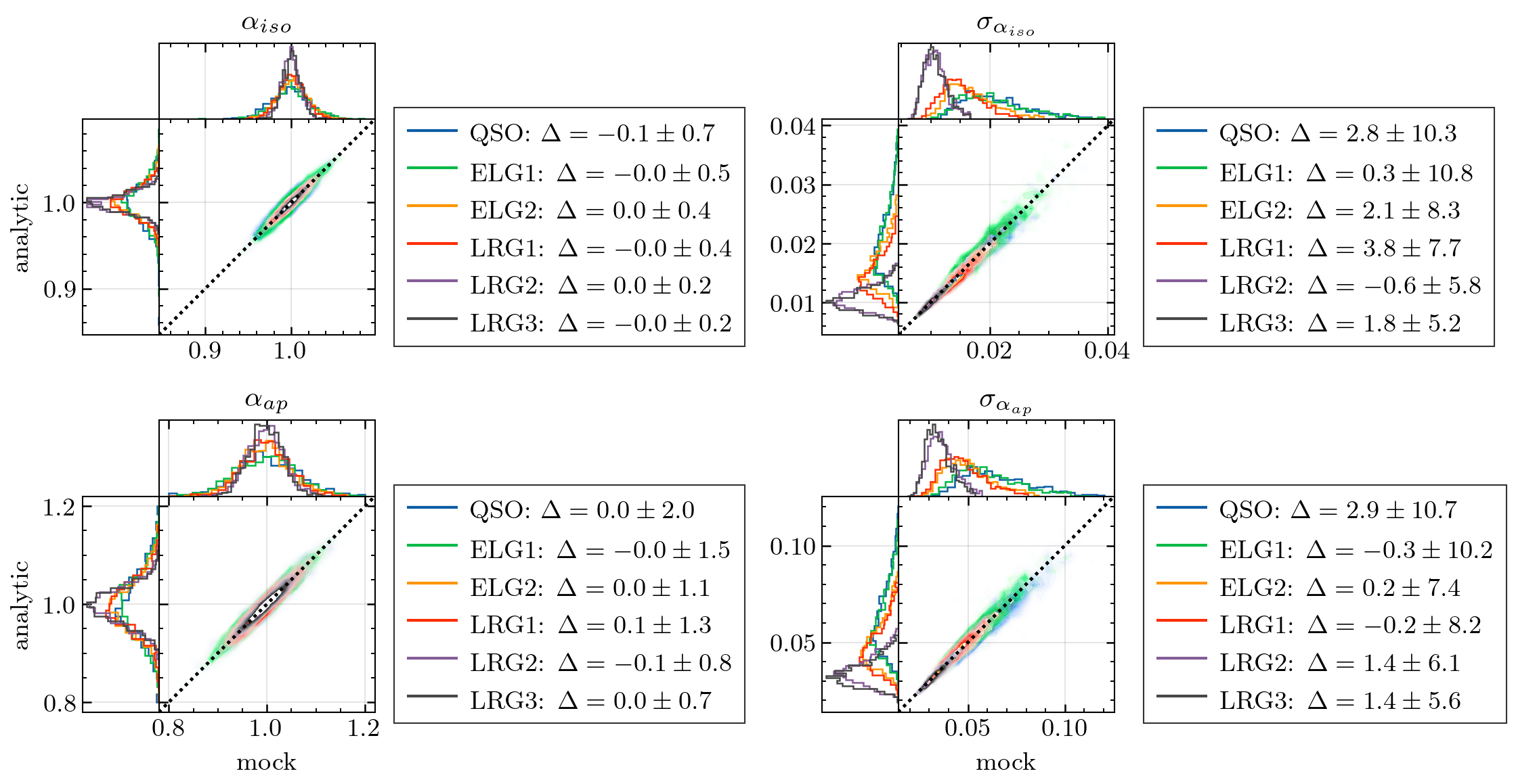
Figure 2: Comparison of fits using the RascalC semi-analytical and mock-based covariance matrices. The figure demonstrates the consistency of the inferred distance scales and errors using our two approaches for computing the covariance matrices. The panels on the left show the BAO distance scales $\alpha_{\rm iso}$ and $\alpha_{\rm AP}$, while the panels on the right show the errors on these parameters. The $x$-axis show results using the mock-based covariances in the fits, while the $y$-axis show results using the RascalC semi-analytical covariances. The RascalC matrices have been tuned to the ensemble of mocks. Further tests were performed using matrices tuned to a single mock which yield consistent results. The $\Delta$ values in the legends on the left show the fractional mean and standard deviation (in percent, relative to the analytic value) of the difference between the $\alpha$ values, while the values on the right correspond to the difference in the errors.

Our analysis here has used both analytic and mock-based approaches to computing the covariance matrices for the two-point functions. We summarize the construction and validation of these covariance matrices below.

The analytic covariances assume Gaussian covariances based on the observed clustering of the galaxies and account for the effects of the survey geometry and selection function. Note that while we largely limit to the disconnected terms, these are derived from the observed nonlinear clustering of the data or mocks.

The covariance matrices for the correlation functions are generated with the RascalC code[130, 131, 132, 133], a variant of which was used for the BAO analysis of the early DESI data [134]. In addition to the disconnected term, the code also includes an adjustable shot-noise parameter that serves as a proxy for the missing connected 4-point terms in the covariance matrix. This parameter can be calibrated with data jackknife resampling (or mocks). A complete discussion of this method is in [49], along with the validation of the data pipeline on mocks demonstrating high consistency with their sample covariance, in particular for errorbars of BAO scale parameters. The code used to generate the covariance matrices for this analysis is publicly available.

The covariances for the power spectrum are based on the formalism by [135]. Our implementation is described in detail in [50]. For the power spectrum we limit to the Gaussian terms and do not include any higher-order corrections.

In addition to the analytic covariances, we also use the EZmocks described previously to generate sample covariance matrices. The advantage of the EZmocks covariances is that we can directly assess the impact of observational systematics like fiber assignment. These mocks are used to test the approximations made in the generation of the analytic covariance matrices. A detailed comparison of the two approaches for generating covariance matrices is in [48]. In particular, we quantify how the fitting of the BAO scales and the corresponding errors depends on the choice of the covariance matrix used. Figure 2 compares the $\alpha$ values and their errors for the full sample of mocks obtained from fits in configuration space. We find that the analytic and mock-based covariances yield answers that are consistent to (much) better than 0.1% for $\alpha_{\mathrm{iso/AP}}$ and generally $<2\%$ for the errors. Both these values sit comfortably within the respective standard deviations for all the galaxy samples. Note that, in addition to the consistent average BAO scales and average errors between the two types of covariance matrices, the individual measurements demonstrate high correlation, typically ranging between 0.965-0.980, as depicted by the distribution thickness in Figure 2. We stress that these tests are done using analytic covariances tuned on EZmocks, thus making the sample covariance baseline a fair estimate of the true covariance. While Figure 2 shows results for a matrix built using the mean of EZmock clustering and the shot-noise rescaled for an optimal match to the sample covariance, [48] shows that such a matrix is consistent with matrices built from a single EZmock realisation and the shot-noise rescaling based on a jackknife covariance estimate as is done using observational data.

A caveat is that we have not attained the desired level of agreement between the analytic and the EZmock covariance matrices in Fourier space as of the time of writing this paper, as will be presented in [48]. Hence, we consider our default results in configuration space the most robust measurements.

Given this level of agreement, particularly in configuration space, we adopt analytic covariance matrices built based on the unblinded DESI DR1 data and calibrated using jackknife resampling of this same data for our analyses in this paper. This choice allows us to tune our covariances to match the observed clustering of the data after we unblind the data, and to avoid the small discrepancies between the clustering seen in the data and the mocks. We note that we are focusing on the BAO observables here, although preliminary work seems to suggest that the analytic covariances may also work well for other observables, at least on large scales.

5 Systematic Error Budget

This section provides an overview of the systematic errors on the BAO scales stemming from various components of our analysis pipeline, as determined through the tests performed in our supporting papers (Table 1). Although individual supporting papers may use a more stringent limit for investigating systematics, the overarching rule we use is to count systematics when we detect an effect that exceeds $3\sigma$, compared to the statistical error associated with the mock test. We will conclude this section by presenting the combined systematic errors on the BAO scales.

Name/Description	$\sigma_{\alpha_{\mathrm{iso}}}$	$\sigma_{\alpha_{\mathrm{AP}}}$
Non-linear mode-coupling	$<0.1\%$	$<0.1\%$
Relative velocity effects	$<0.05\%$	$<0.05\%$
Broadband modelling	$<0.02\%$	$0.11\%$
BAO wiggle extraction	$<0.02\%$	$<0.09\%$
Dilating smooth vs. wiggle	$<0.02\%$	$<0.09\%$
Modelling $\xi(s)$ from $P(k)$	$<0.01\%$	$0.12\%$
Combined	$0.1\%$	$0.2\%$

Table 7: Different contributions to the DESI galaxy BAO theory and modelling systematic error budget for $\alpha_{\mathrm{iso}}$ and $\alpha_{\mathrm{AP}}$ considered in this work, taken from [7]. The first two rows denote theory cases, where the exact contributions depend on the nature of the tracers (galaxy bias, redshift, etc.), we have estimated a conservative upper value considering all DESI tracers/redshift bins. The other rows are obtained from fitting the Abacus-1  cubic, control-variate (CV) measurements while varying our modelling assumptions/choices. Only two of the tests show that our results can potentially be subject to a small nonzero bias. The remainder return no difference within the statistical precision available from the simulations and so are reported as upper bounds. The combined theory and modelling systematic error is obtained by summing the two solid detections in quadrature and rounding up to account for the remaining upper limits.

5.1 Theoretical Systematics

Ref. [7] investigates the systematic error induced by various approximations made when modelling the BAO. These can potentially arise from either physical effects that are dropped from the model used in BAO fits, e.g., the shrinkage of the BAO feature due to non-linear clustering/evolution in the galaxy distribution [136, 137, 138, 139, 140] or the imprint of relative baryon-dark matter perturbations. There can also be residual errors due to (small) imperfections in the numerical choices made in the broadband model and extraction of the BAO template.

The physical processes affecting the BAO feature are comprehensively computed in [7] within perturbation theory. The impact of the numerical choices made in the modeling is measured by fitting to our high-precision Abacus-1 cubic, control-variate (CV) measurements while changing the numerical prescriptions used in the modelling. The robustness of the BAO means that even with the large volume and sample-variance cancellation of the Abacus-1 cubic mocks most of the modelling choices we test give consistent constraints within the statistical uncertainties, and we report only upper bounds on the potential systematic error. We obtain positive detections of only two (small) systematic modelling errors. The first arises from comparing our preferred spline-based broadband model with the historically used polynomial-based model. The second arises from comparing our new approach of modelling the correlation function as the Hankel transform of the dilated power spectrum multipoles with free growth rate parameter, to the BOSS approach [20] of transforming the undilated multipoles and applying the dilation after the transformation, then varying two different bias parameters for the monopole and quadrupole rather than the growth rate parameter. In both cases, we argue that our new method is better physically motivated and preferred, but as these are nonetheless modelling choices that also passed the systematic checks used in previous studies, we absorb these differences into our systematic error budget.

Using these two detections, upper bounds on the other modelling considerations, and folding in the expected theoretical upper limits from nonlinearities, we obtain a (conservative) systematic error on $\alpha_{\rm iso,ap}$ of $0.1$ and $0.2\%$, respectively. The different contributions to this total are in Table 7.

	Parameter	$\sigma_{\text{HOD,BGS}}$	$\sigma_{\text{HOD,LRG}}$	$\sigma_{\text{HOD,ELG}}$	$\sigma_{\text{HOD,QSO}}$
$P(k)$	$\alpha_{\rm iso}$	0.19%	0.066%	0.047%	0.12%
	$\alpha_{\rm AP}$	—	0.094%	0.089%	—
$\xi(r)$	$\alpha_{\rm iso}$	0.20%	0.074%	0.17%	0.07%
	$\alpha_{\rm AP}$	—	0.187%	0.11%	—

Table 8: Summary table for the estimation of HOD-dependent systematics for individual tracers. The table is split into Fourier and configuration space results, and we include the systematics for both $\alpha_{\rm iso}$ and $\alpha_{\rm AP}$. The results for LRGs and ELGs are presented in detail in [52] and [53]. The results for BGS and QSO are derived consistently to LRGs and ELGs. The bold-faced numbers indicate a detection of systematics; otherwise, the numbers reflect the statistical precision associated with no detection. As conservative upper limits, we adopt systematic error on $\alpha_{\rm iso,ap}$ of $0.1$ and $0.2\%$ for the HOD-dependent systematics.

5.2 HOD-dependent systematics

Systematic errors can be introduced when we infer the underlying BAO scale in the matter density field from the BAO measurement using a specific choice of LSS tracer, which is typically a biased tracer. Studies have shown that such systematics are subdominant compared to the shift in the BAO scale due to structure growth and redshift-space distortions; moreover, they effectively vanish after reconstruction [141]. Given the precision of the state-of-the-art DESI DR1 data and that the new major tracer, the ELGs, believed to exhibit distinct halo occupation features compared to LRGs, this test is revisited. Our supporting papers, [52] and [53], extensively test the systematics for the different assumptions of the halo occupation distribution (HOD) for LRGs and ELGs, respectively, using DESI mock catalogs constructed from Abacus simulations. [52] studied nine different variations of HODs that are within $3\sigma$ of the best-fit HOD parameters to the One-Percent Survey [80]. [53] studied the impact of the ELG HODs using 22 different HOD models, including the standard models used for Abacus-1 and Abacus-2 as well as extended models that include galactic conformity, assembly bias, and modified satellite profile adopted from [89].

The amplitude of HOD systematics is estimated using the same methodology in both of our supporting papers, [52] and [53]. We compute the differences in $\alpha_{\rm iso}$ and $\alpha_{\rm AP}$ between every pair of HOD models, averaging over the 25 realizations. We compute the significance of this difference to assess the systematic detection level. If we do not detect systematics at the level of 3$\sigma$ in terms of the typical dispersion of the average differences from the mocks, we use the distribution of the differences between all pairs of HOD models and quote the 68% region of the distribution as the systematic error. On the other hand, if any of the paired HODs shows a non-zero difference at 3$\sigma$ or above, we take the shift between that pair of HODs as the systematic error. If there is more than one pair of HODs with a non-zero difference above 3$\sigma$, we quote the maximum of these shifts. Table 8 shows the summary of the systematics for each tracer. The systematics for BGS and QSO are derived consistently.

Note that the quoted systematic error, in the case of no detection, often merely reflects the limited sample variance cancellation due to the different subsampling noise. Even for the detection cases, an analysis like this depends on how extreme the HOD models we decide to compare are; we compare the models that span the $\pm 3\sigma$ contours around the best-fit HODs, which is a reasonable choice to incorporate viable HOD parameter values allowed by the data. In addition, this test includes the systematics in the process of reconstruction as well, as we fix the galaxy bias input to reconstruction, while the actual HOD model (and, therefore, the effective bias) is being varied, with variations with respect to the input bias scaling up to 10%. The theoretical systematics reported by [7] already include a contribution due to the reference HOD model assumed in the simulation they utilized, and therefore the HOD systematics reported in this section should be considered as additional systematics on the BAO scales that can be introduced by assuming different HODs than the reference HOD model tested in [7].

Using the results presented in Table 8, we adopt a conservative approach and consider a common HOD-dependent systematic error for all tracers of 0.2% for both $\alpha_{\rm iso}$ and $\alpha_{\rm AP}$.

5.3 Observational Systematics

Similar to results found in SDSS (e.g., [142]), we find that observational systematics have a negligible impact on our BAO measurements. We therefore do not add any additional observational systematic uncertainty. We briefly outline the studies justifying this conclusion.

Tracer	Recon	$\langle\alpha^{\rm complete}_{\rm iso}\rangle$	$\langle\alpha^{\rm complete}_{\rm AP}\rangle$	$\langle\alpha^{\rm complete}_{\rm iso}-\alpha^{\rm altmtl}_{\rm iso}\rangle$	$\langle\alpha^{\rm complete}_{\rm AP}-\alpha^{\rm altmtl}_{\rm AP}\rangle$
${\tt BGS}$	Post	$0.9998\pm 0.0038$	—	$0.00288\pm 0.00229$	—
${\tt LRG1}$	Post	$0.9996\pm 0.0025$	$0.9934\pm 0.0091$	$-0.00182\pm 0.00163$	$0.00374\pm 0.00455$
${\tt LRG2}$	Post	$0.9967\pm 0.0022$	$1.0091\pm 0.0075$	$0.00207\pm 0.00144$	$0.00096\pm 0.00392$
${\tt LRG3}$	Post	$0.9958\pm 0.0019$	$0.9854\pm 0.0063$	$0.00240\pm 0.00161$	$-0.00407\pm 0.00512$
${\tt ELG1}$	Post	$1.0015\pm 0.0035$	—	$0.00118\pm 0.00422$	—
${\tt ELG2}$	Post	$0.9988\pm 0.0030$	$1.0025\pm 0.0100$	$0.00387\pm 0.00270$	$0.00387\pm 0.00676$
${\tt QSO}$	Post	$0.9968\pm 0.0033$	—	$0.00207\pm 0.00361$	—

Table 9: The mean and the error associated with the mean of the BAO measurements from the 25 Abacus-2 DR1 mocks using the DESI DR1 baseline BAO method, as presented in [46]. Results indicate that fits to the ‘complete’ mocks, i.e., before applying fiber assignment effects, align with unbiased BAO measurements within statistical error. Furthermore, the mean difference between the  altmtl mocks and the ‘ complete’ mocks demonstrates the recovery of unbiased BAO estimates despite the presence of the fiber assignment effect. LRG3$+$ELG1 is omitted since it is the combination of LRG3 and ELG1.

Observational systematics in DESI can be broadly divided into three classes: fiber assignment incompleteness, spectroscopic systematics, and imaging systematics. Any effects of fiber assignment incompleteness can be tested by comparing results on our DR1 mocks (described in Section 3) that have no fiber assignment incompleteness (‘complete’) and those that have had fiber assignment run in a way that mimics the DESI DR1 observing history (‘altmtl’). Each have been run through the DESI DR1 BAO measurement pipeline and consistent results were found [46], as summarized in Table 9. The table first shows that the BAO fits from Abacus-2 DR1 ‘complete’ mocks are consistent with no bias. The altmtl mocks are consistent with the ‘complete’ mocks within 1.5$\sigma$, demonstrating that we can recover unbiased BAO measurements in the presence of the fiber assignment. The differences in $\alpha_{\rm iso}$ appear systematic. The weighted mean (assuming no correlation) is $\langle\alpha^{\rm complete}_{\rm iso}-\alpha^{\rm altmtl}_{\rm iso}\rangle_{\rm all}=0.00149\pm 0.00077$ and thus just under 2$\sigma$. This is not significant enough for us to add as a systematic uncertainty, but does suggest a closer look is warranted in future DESI studies.

Significant trends between the observed DESI galaxy density and the observational properties of the imaging data used to define the target samples (e.g., the imaging depth) are found for all DESI tracers [96]. These trends are removed from the DR1 LSS catalogs via weights that are added to the sample based on regression analysis against maps of the observational properties. The overall impact of the weights on the DR1 clustering measurements is quite large in significance; the $\chi^{2}$ difference between weighted and unweighted clustering for ELGs is greater than 1000 [23]. However, the impact on BAO measurements is negligible, as shown in Figure 3. When comparing the post-reconstruction BAO measurements with and without weights to correct for imaging systematics, the variation is found to be at most $0.27\sigma$ (for the QSO $\alpha_{\rm iso}$) and is typically less than $0.2\sigma$ on any of the measured BAO parameters ($\alpha_{\rm iso}$ and $\alpha_{\rm AP}$), without any coherent direction across tracers. The weights modulate the density field obtained from the LSS catalogs and thus there is expected to be some fluctuation in any measured parameter that is proportional to the original uncertainty, purely from the degree to which the weighting de-correlates the weighted and unweighted data. Thus, shifts as a fraction of the uncertainty on the measured BAO parameters are the most relevant thing to quote here. The 0.2$\sigma$ level of variation is equivalent to a correlation of 0.99 between the weighted and unweighted results. This is thus similar to that one would expect from randomly applying weights with the same variance as the imaging systematic weights to the sample. We stress that the weighted clustering results are expected to be much closer to the ‘true’ clustering than those without the imaging systematic weights. Thus, even if these shifts were not consistent with random variation, they would represent an extreme scenario.

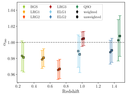
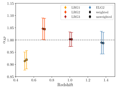
Figure 3: The impact of imaging systematics on the BAO scales. In detail, we show the difference in the derived BAO scales when we use the mitigation method for imaging systematics and when we use the raw data (‘No weight’). The two measurements for each tracer are slightly displaced horizontally for a better visualization. The BAO scales are very stable even when there was no mitigating and even after density field reconstruction using such raw data. Again, the BAO is robust against the imaging systematics.

Spectroscopic systematics refer to both the effect of errors in the DESI redshift estimation and unphysical galaxy/quasar variations in the fraction of successful redshifts as a function of parameters relating to DESI hardware and observing conditions. Similar to the corrections for imaging systematics, trends with spectroscopic properties can be regressed against, and corrected with, weights. Such weights, $w_{\rm zfail}$, are determined as a function of effective observing time for all DESI tracers, as described in [24, 71]. Despite the significance of the observed trends, [24] find that difference in clustering between results including $w_{\rm zfail}$ or not yields a maximum $\chi^{2}$ difference of just 0.09 (for ELG samples at both redshift range) across all of the pre-reconstruction $\xi_{0,2}$ within the BAO fit range. Such a small $\chi^{2}$ difference implies at most a 0.3$\sigma$ shift in any potential parameter; the differences are not localized and any effect on BAO measurements is thus expected to be negligible. Further corrections, such as extra weights to remove the remaining dependence of the success rate on the focal plane location, were also studied in [24] and found to have similarly small effects on the measured clustering. The size of the effect of redshift success trends on the DESI DR1 two-point functions is thus negligible for BAO measurements.

Finally, redshift errors have been characterized again in DR1. These are divided into two components: a typical uncertainty, characterized by a narrow Gaussian or Lorentizian profile, and a rate of catastrophic failure. The potential impact of the typical uncertainty on clustering measurements have been studied with galaxy mocks generated with the UNIT-SHAM method [143] and AbacusSummit-HOD models [80, 89]. In [143] the impact on ELGs was negligible at all scales and the effect for LRGs was $\sim 0.05\sigma$. In DR1, the ELG redshift uncertainty is even smaller [24], and LRGs show the same level of uncertainties [71]. The impact on measured QSO clustering was substantially greater, due to the larger uncertainty on their redshifts. However, the effect of redshift uncertainties as an additive component to the velocity dispersion is included for both LRG and QSO in the DESI Y1 mocks, where no detectable bias in BAO parameters is found.

In studying catastrophic failures in the redshift measurements of DESI ELGs (using, e.g., repeated observations of the same ELG), [24] find that the most prominent feature is confusion at $z\sim 1.32$ between residuals from sky spectra and [O ii] emission. The total failure rate from repeat spectra was found to be 0.27%, much smaller than the worst case of 1% [144]. However, the observed failure patterns with 0.27% rate show similar clustering impacts to the assumed 1% failures for ELG mocks at $1.1<z<1.6$ due to the prominent confusion at $z\sim 1.32$. Nevertheless, their impact on the measured configuration space clustering is $<0.01\sigma$ at scales $s>60\ h^{-1}\text{Mpc}$ and thus should not impact BAO measurements.

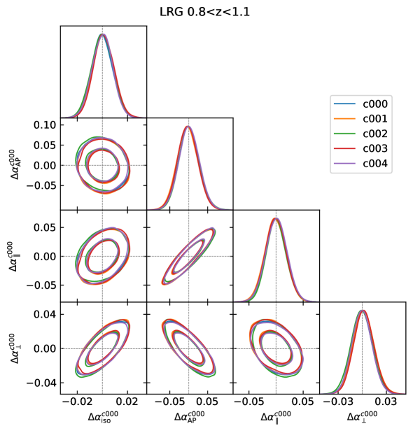
Figure 4: Contour plots of the differences of the (rescaled) alpha values measured with the different AbacusSummit cosmologies using DESI DR1 data. As an example, the LRG high redshift bin is shown. The quantities $\Delta\alpha^{c000}$ are defined as follows. For a given cosmology c00x, the derived alpha values are rescaled to c000 units and the values measured directly with c000 are subtracted.

5.4 Systematics due to the assumption of the fiducial cosmology

In this subsection, we summarize the impact of using a wrong fiducial cosmology in the BAO analysis, which were extensively studied in [51].

The choice of reference cosmology comes into play at three different stages. First, we assume a set of cosmological parameters when converting redshift measurements into distances; we term this the grid cosmology. The difference between the grid and true cosmologies causes a distortion of the BAO scale along and across the line of sight [10], which is quantified by the parameters $q_{\parallel}=H_{\textrm{grid}}(z)/H_{\textrm{true}}(z)$ and $q_{\perp}=D_{\textrm{true}}(z)/D_{\textrm{grid}}(z)$ respectively. Without the three-dimensional standard ruler like BAO, this effect is somewhat degenerate with the redshift-space distortions, but with a sufficiently large data set, such as we have with DESI, and with the BAO feature it is possible to distinguish between the two [145, 146]. Second, a template cosmology is chosen in order to compute the linear power spectrum, which is then used to create the model power spectrum for the fitting ($P_{\rm nw}$ and $P_{w}$ in Eq. 4.1). The effect of fixing the template is interpreted as an additional isotropic rescaling of the distances by a factor of $r_{d}^{\rm tem}/r_{d}^{\rm true}$. Lastly, the values for the linear bias $b_{1}$ and the growth rate $f(z)$ input into the reconstruction algorithm are cosmology dependent, affecting the estimation of the displacement field. The separate effect of both the template and the values assumed for reconstruction have been comprehensibly studied in the past [147, 148, 149, 150], as well as the joint effect of consistently changing the reference cosmology in the whole pipeline [114], while the separate effect of the grid is less explored [151]. Potential systematic shifts of the order of a few tenths of a percent in the alpha values have been reported in the most extreme scenarios.

We studied the effect of analysing mocks with DESI DR1 geometry with different fiducial cosmologies. Namely, the four secondary AbacusSummit [152] cosmologies (Table 10), which deviate from the Planck 2018 cosmology in various aspects. For example, from Table 10, c002 introduces an offset on the distance to redshift relation at the level of $\sim 4.7-7.5$% and an offset in the sound-horizon scale at the level of 6.8%. Up to 2.9% of the anisotropic distortion (AP) is also tested with c002.

Our baseline test consists of simultaneously changing the cosmology for grid, template and reconstruction (the separate contributions of grid and template are explored in the companion paper). The fiducial DESI cosmology c000 is used to create the Abacus-2 DR1 mock catalogs, but the different grid cosmologies c001-c004 are used to convert redshifts into distances to compute the pair counts and power spectrum. The change in template is implemented by simply changing the linear power spectrum computed with class and then following the fitting procedure with desilike as described in Section 4.3. The values for the linear bias and growth rate are derived assuming each fiducial cosmology and introduced in reconstruction.

We compare the expected BAO scales (the last two columns in Table 10) with the derived BAO scales for all tracers and for each of the wrong fiducial cosmologies using 25 Abacus-2 DR1 mocks, and regard a shift detection for values above a 3$\sigma$ based on the dispersion of the 25 mocks. Table 11 summarises our results in [51]. For cosmology c003 we measure a systematic shift of the order of 0.2% for $\alpha_{\rm iso}$ that can be neatly explained by the phase shift in the BAO due to the difference in $N_{\rm eff}$ (see for example [153]). Since this effect comes from the template and it is a matter of how the re-scaling by the sound horizon is interpreted in the BAO measurements, we opt to not include it as part of the systematic error budget. A detection at the level of 0.1% is reported for c002 from [51]; otherwise we do not see a detection of bias. Thus we adopt a conservative value of 0.1% for both $\alpha_{\rm iso}$ and $\alpha_{\rm AP}$. Furthermore, we tested the consistency of the BAO fits against the choice of fiducial cosmology for the blinded Y1 catalogs, as part of the unblinding tests described in Table 14. Likewise, we conduct an analogous comparison with the unblinded data, for which consistent results are observed for the different cosmologies (Figure 4).

Cosmology	Description	$\frac{r_{d,\rm tem}}{r_{d,\rm true}}$	$\frac{\alpha_{\rm iso,fid}}{\alpha_{\rm iso,true}}$	$\frac{\alpha_{\rm iso,fid}}{\alpha_{\rm iso,true}}$	$\frac{\alpha_{\rm AP,fid}}{\alpha_{\rm AP,true}}$
		(template)	(grid)	(template + grid)	(grid)
c000	Planck 2018 $\Lambda$CDM	1.000	1.000 – 1.000	1.000 – 1.000	1.000 – 1.000
c001	Low $\omega_{c}$ $\Lambda$CDM	1.056	0.963 – 0.989	1.017 – 1.044	0.976 – 0.991
c002	Thawing dark energy	0.932	1.047 – 1.075	0.976 – 1.002	1.011 – 1.029
c003	$N_{\rm eff}=3.70$	1.022	0.983 – 0.995	1.005 – 1.017	0.989 – 0.996
c004	$\sigma_{8}=0.75$ $\Lambda$CDM	1.000	1.000 – 1.000	1.000 – 1.000	1.000 – 1.000

Table 10: The level of scale dilation and anisotropy on the $\alpha$ parameters we introduce in the test of the fiducial cosmology, by adopting four fiducial cosmologies (c001-c004) when analyzing the mock catalogs generated using the true cosmology (c000). Each of c000-c004 is based on AbacusSummit[152]. The effect of the grid cosmology on the scale dilation depends on redshift and we therefore list the ranges for $0.1<z<2.1$. Note that, with c002, we introduce an offset on the distance to redshift relation at the level of $\sim 4.7-7.5$% and an offset in the sound-horizon scale at the level of 6.8%. Up to 2.9% of the anisotropic distortion (AP) was also tested with c002. The last two columns are the expected BAO scales we should recover. A significant (3$\sigma$) offset of the derived BAO scale from the last two columns is considered as a bias.

Space	Parameter	c000-c00X	c000-c003
Fourier	$\alpha_{\rm iso}$	0.1%	0.2%
	$\alpha_{\rm AP}$	None (0.1%)	None (0.1%)
Config.	$\alpha_{\rm iso}$	None (0.1%)	0.2-0.3%
	$\alpha_{\rm AP}$	None (0.1%)	None (0.1%)

Table 11: Estimation of systematics due to the assumption of an incorrect fiducial cosmology, based on the test by [51]. We show the residual bias in the BAO scales after accounting for the expected shift due to using incorrect grid and template cosmologies (c00X, where $X=1$, 2, 4). Unless the residual bias in the BAO is detected at a significance greater than $3\sigma$ (in terms of the standard deviation of the mean of the mocks), we consider there to be no net bias in the BAO scale due to the fiducial cosmology and put an ad-hoc value of 0.1%. We detected a significant bias in $\alpha_{\rm iso}$ for c003, which assumes an incorrect $N_{\rm eff}$ in the BAO template. Systematics from an incorrect $N_{\rm eff}$ are not included in our systematic budget, as this concerns the interpretation of the measured BAO scale.

5.5 Combining all systematics

Systematic	Error (in percent)	Comments
Theoretical	0.1 ($\alpha_{\rm iso}$), 0.2 ($\alpha_{AP}$)	Includes fitting methodology and choices,
		as well as expected impacts from
		galaxy bias and cosmology misestimation
Observational
a. Imaging	Not detected	Tested on the data, with the
		largest change being 0.3% seen for the
		ELG1, and the rest being 0.1%.
b. Spectroscopic	Not detected	Tested with the mocks on the clustering level.
c. Fiber assignment	Not detected	The test was finalized after unblinding.
HOD	0.2	Only one detected statistically significant pair
		Limited by statistical precision of mocks
		Note : some of this error is already included in
		the theory budget
$N_{\rm eff}$	0.2 ($\alpha_{\rm iso}$)	Bias for $N_{\rm eff}=3.7$
Fiducial $D_{A}(z)$	$<0.1$	May require iteration post-unblinding
		if best-fit is far from fiducial
		Upper limit based on statistical precision
Reconstruction	Not detected	No significant effects from different
		algorithms etc.
Covariances	Not detected	Based on comparisons between analytic
		and mock covariances

Table 12: Summary of our individual systematic errors. In some cases, we do not have any statistically significant detection of a systematic bias.

	Tracer	$\sigma_{\text{BGS}}$	$\sigma_{\text{{\tt LRG}s,{\tt ELG}s}}$		$\sigma_{\text{QSO}}$
Space	Source	$\alpha_{\rm iso}$ (%)	$\alpha_{\rm iso}$ (%)	$\alpha_{\rm AP}$ (%)	$\alpha_{\rm iso}$ (%)
$\xi(r)$	Theory (Table 7)	0.1	0.1	0.2	0.1
$\xi(r)$	HOD (Table 8)	0.2	0.2	0.2	0.2
$\xi(r)$	Fiducial (Table 11)	0.1	0.1	0.1	0.1
$\xi(r)$	Total	0.245	0.245	0.3	0.245
$P(k)$	Theory (Table 7)	0.1	0.1	0.2	0.1
$P(k)$	HOD (Table 8)	0.2	0.1	0.1	0.12
$P(k)$	Fiducial (Table 11)	0.1	0.1	0.1	0.1
$P(k)$	Total	0.245	0.18	0.245	0.19

Table 13: The combined non-zero systematics. The total error in each space is obtained by summing contributions in quadrature and rounding to two significant digits. For the fiducial cosmology systematics, we do not include the bias that can be introduced due to an incorrect assumption of $N_{\rm eff}$ in the fitting model. Although the tracer-by-tracer estimation of the systematics, such as the HODs, return smaller systematics for some tracers and in $P(k)$, here we will adopt the worst case of the systematics across all tracers, $0.245\%$ for $\alpha_{\rm iso}$ and 0.3% for $\alpha_{\rm AP}$ for both $\xi(r)$ and $P(k)$.

In this subsection, we combine all the systematics in the basis of $\alpha_{\rm iso}$ and $\alpha_{\rm AP}$, and then project these to the systematics in $\alpha_{\perp}$ and $\alpha_{\parallel}$. It is imperative to include all pertinent systematics, while setting the upper limit of systematics conservative enough to avoid adding systematics after unblinding.

The summary of the systematic tests is in Table 12. From [45, 46], we conclude that the systematics due to the reconstruction choice, within a few comparably optimal options we narrowed down, is negligible. Moreover, the systematics due to incorrect estimation of bias and incorrect fiducial cosmology during reconstruction are already accounted for by the HOD systematics (Table 8) and the fiducial cosmology systematics budgets (Section 5.4). We also conclude that the observational effects (Section 5.3) and the covariance choice (Section 4.5 and [48]) are negligible.

Table 13 shows the combination of all systematic budgets based on Table 12. We opt for the most conservative approach, namely, directly adding in quadrature individual systematic budgets. This approach only marginally increases the final error by $\sim$5% even for the best $\alpha_{\rm iso}$ measurement.

Assuming the negligible correlation between the systematics in $\alpha_{\rm iso}$ and $\alpha_{\rm AP}$, which was the reason we have been evaluating the systematics using this basis, we derive

$$\mathcal{C}^{\rm Sys}_{\rm\alpha_{\rm iso},\alpha_{\rm AP}}=\begin{pmatrix}0.245^{2}&0\\ 0&0.3^{2}\end{pmatrix},$$ (5.1)

where the matrix elements are the fractional (%) covariances.

We projecting this to the systematics in $\alpha_{\perp}$ and $\alpha_{\parallel}$ following

$${\rm C}^{-1}_{q_{i}q_{j}}=\frac{d\ln p_{a}}{d\ln q_{i}}\mathcal{C}^{-1}_{p_{a},p_{b}}\frac{d\ln p_{b}}{d\ln q_{j}}$$ (5.2)

where $q_{i},q_{j}=\alpha_{\perp},\alpha_{\parallel}$ and $p_{a},p_{b}=\alpha_{\rm iso},\alpha_{\rm AP}$. With $\mathcal{C}_{p_{a},p_{b}}=\mathcal{C}^{\rm Sys}_{\rm\alpha_{\rm iso},\alpha_{\rm AP}}$ and

$$\frac{d\ln p_{a}}{d\ln q_{i}}=\begin{pmatrix}2/3&1/3\\ -1&1\end{pmatrix},$$ (5.3)

we find

$${\rm C}^{\rm Sys}_{\alpha_{\perp},\alpha_{\parallel}}=\begin{pmatrix}0.265^{2}&0.478(0.265\times 0.316)\\ 0.478(0.265\times 0.316)&0.316^{2}\end{pmatrix}.$$ (5.4)

This again is the fractional (%) covariances. For the best BAO measurement, LRG3$+$ELG1, this increases an error on $\alpha_{\parallel}$ by 1.5% and $\alpha_{\perp}$ by 2.2%.

Note that, unlike the statistical constraints in Table 15, this synthetic matrix for systematics (Eq. 5.4) shows a positive cross-correlation, which is mainly because the variances in $\alpha_{\rm iso}$ and $\alpha_{\rm AP}$ are more comparable, unlike the statistical constraints that are subject to a particular combination of contribution of transverse and parallel wavemode. We add $\mathcal{C}^{\rm Sys}_{\rm\alpha_{\rm iso},\alpha_{\rm AP}}$ and ${\rm C}^{\rm Sys}_{\alpha_{\perp},\alpha_{\parallel}}$ to the corresponding statistical BAO covariance to construct the final posteriors.

6 The Unblinding Tests

Test	Results
$\chi^{2}$ acceptable?	Yes
$\alpha$ consistent between pre and post?	Yes
$\alpha$ consistent between NGC+SGC and NGC?	Yes
Consistency between North and South?	Tested at the level of the clustering (Section 2)
$\alpha$ consistent across different fiducial cosmologies?	Yes
$\alpha$ consistent between $\xi(r)$ and $P(k)$?	Yes
Are the error bars reasonable?	Consistent with the mocks
$\alpha$ consistent between LRG and ELG $0.8<z<1.1$	Yes

Table 14: Unblinding checklists. For each entry in the checklist, if the difference observed in the blinded data is within the full range covered by the 25 Abacus-2 DR1 mocks, we consider that the test was passed. For BGS, ELG1, and QSO, 1-D BAO fits pass these tests while the other tracers pass these tests with 2-D as well as 1-D fits.

One manifestation of confirmation bias is the tendency to attribute a higher level of systematic uncertainty to outcomes that are unexpected or perceived as outliers. To prevent this from affecting the DESI DR1 BAO measurements, we determined the systematic error budget detailed in Table 12 prior to unblinding.

Before unblinding, we also required the following set of the conditions to be met.

1. The official DESI DR1 galaxy BAO analysis pipeline must be determined, including the density field reconstruction setup and the BAO fitting setup. We determined these configurations based on the tests on the blinded data and the mocks. These mocks were calibrated against the DESI One Percent sample rather than DESI DR1. While this was a limitation potentially affecting optimization for the unblinded data, it was a necessary trade-off due to the blinding process.

2. The consistency tests in the checklist (Table 14) were to have been completed on the blinded data to the fullest extent possible. For each entry in the checklist, if the difference observed in the blinded data is within the entire range covered by the 25 Abacus-2 DR1 mocks, we consider that the test was passed.

Table 14 presents the list of the tests we performed before unblinding. The tests are extensively described in [46]. Based on the tests, we decided the following.

1. We decided the optimal reconstruction scheme and the smoothing scales for each tracer [46]. In particular, we decided to take the reconstructed QSO BAO fit as our fiducial choice regardless of its actual reconstruction efficiency when applied to the unblinded DESI DR1 data.

2. We decided the prior ranges of the BAO damping scales, as detailed in [7].

3. We decided to perform 1-D BAO fits for the lower signal-to-noise samples, i.e., BGS, ELG1, and QSO. 2-D BAO fits on these samples showed either frequent outliers (i.e., failed to locate the BAO) in the mocks or failed some of the consistency tests in Table 14 with the blinded data.

4. We decided to utilize the combined tracer of ELG1 and LRG3  for $0.8<z<1.1$ bin to carry out the cosmology analysis. The information from the lowest signal-to-noise tracer, ELG1, is propagated to cosmological constraints only through the combined tracer analysis.

We also decided on the aspects of the analysis that could be re-done after unblinding.

1. The calibration of covariance matrices could be finalized after unblinding, based on EZmock and analytic covariance matrices. Consequently, the final decision on the covariance matrices between the numerical and analytic covariances could also be made at this stage. This was partly due to the unavailability of EZmocks for DR1 during the unblinding tests, and also because we could not determine beforehand how well the clustering in the EZmocks and Abacus-2 would align with that of the unblinded data.

2. Given the bias expected with an incorrect assumption of $N_{\rm eff}$ in the template (Section 5.4), we allowed a potential iteration of the BAO fits using a different assumption of $N_{\rm eff}$ if we were to find the best fit $N_{\rm eff}$ from the DESI DR1 cosmology analysis different to the value we assumed in the fitting.

3. An update on the catalogs could be made if an error were to be found in checks unrelated to the BAO fitting. The error would then be fixed before assessing the impact of the correction on the BAO fits. As detailed in Section 2.3, an error was indeed identified in the LSS catalogs after unblinding and promptly rectified. The most significant shift on the BAO measurement observed was 0.7$\sigma$ shift in $\alpha_{\rm AP}$ for LRG1, while other shifts are typically less than 0.2$\sigma$.

4. HOD systematics for QSO and BGS would be determined after unblinding, as a result of prioritizing the highest signal-to-noise tracers such as LRGs and ELGs.

After unblinding, we discovered a minor discrepancy between the fitting model outlined in [7] (and Section 4.4 in this paper) and its implementation in the code. The correction of the code resulted in BAO measurement changes of less than a maximum of $0.3\sigma$, with most shifts under $0.1\sigma$, and no systematic correlation in the shifts across redshift bins.

7 Results

In this section, we present the results of the BAO analysis using the unblinded DESI DR1 catalogs.

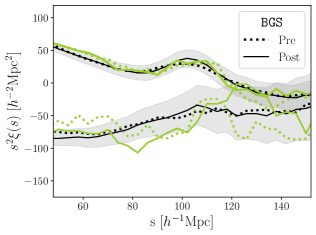
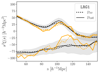
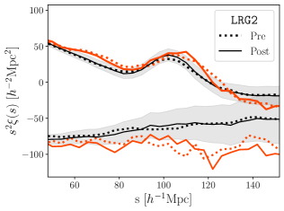
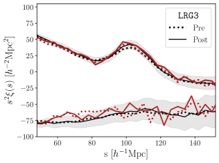
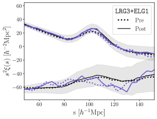
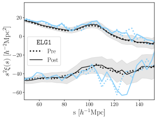
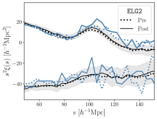
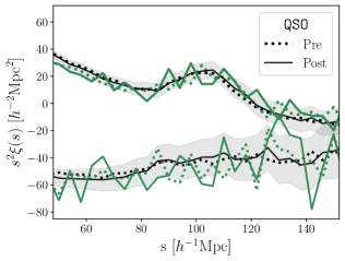
Figure 5: Two-point correlation functions of various tracers of the unblinded DESI DR1 (colored lines). We compare the overall clustering amplitude over the BAO fitting range ($48\ h^{-1}\text{Mpc}<r<152\ h^{-1}\text{Mpc}$) before (dotted lines) and after reconstruction (solid lines), compared to the corresponding mean of the 25 Abacus-2 DR1 mocks (black lines). Gray shading represents the error associated with post-reconstruction DESI DR1 based on RascalC covariance. As a reminder, the data points of $\xi$ are substantially correlated between different separation $r$. The upper set of the lines is for the monopole, and the lower set of the lines is for the quadrupole. The plots demonstrate excellent consistency in the overall clustering between the data and the mocks.

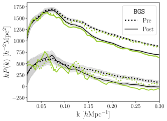
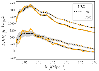
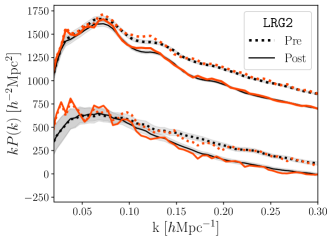
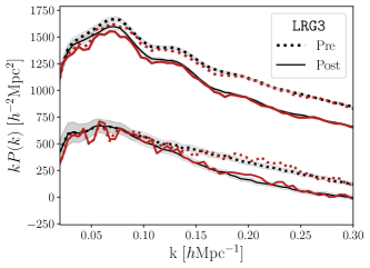
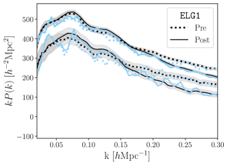
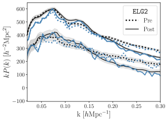
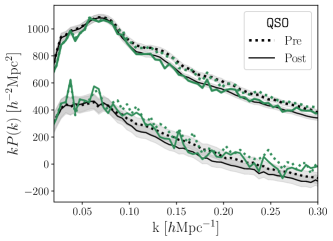
Figure 6: Power spectra multipoles of various tracers of the unblinded DESI DR1 (colored lines) in comparison to the Abacus-2 DR1 mocks (black lines). Similar to Figure 5. The gray shading is from the analytic covariance matrices for the DESI DR1 data in Section 4.5. Again, the plots demonstrate excellent consistency in the overall clustering between the data and the mocks.

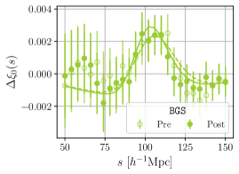
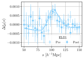
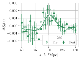
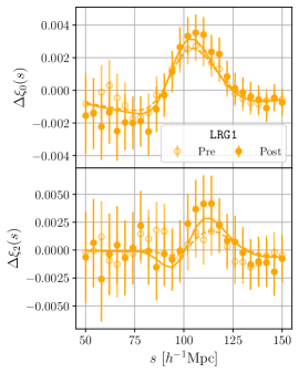
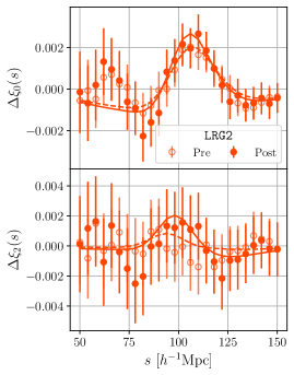
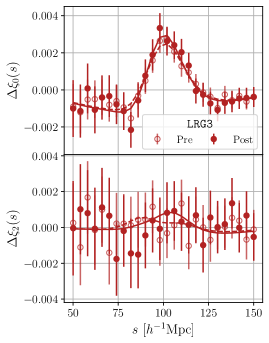
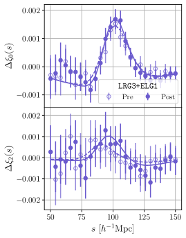
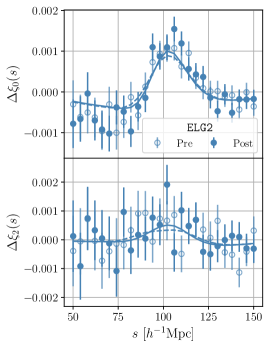
Figure 7: The isolated BAO feature in the correlation function of DESI DR1 data before (open circles) and after reconstruction (solid circles). A 1-D BAO fitting is performed for BGS, ELG1, and QSO, while the rest is fitted for the 2-D BAO scales. The solid and dashsed lines are the best fit BAO models to the unblinded DESI DR1 before (open circles) and after reconstruction (solid circles), respectively.

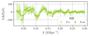
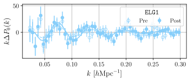
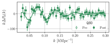
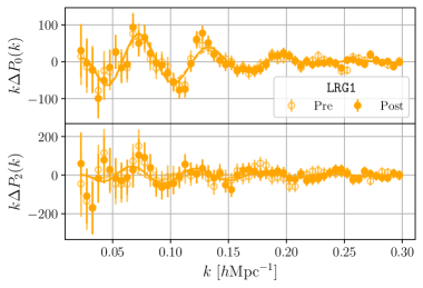
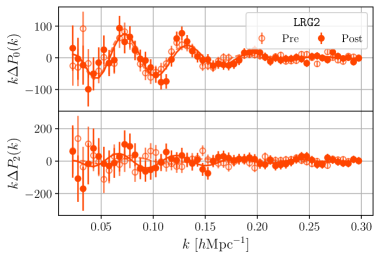
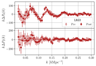
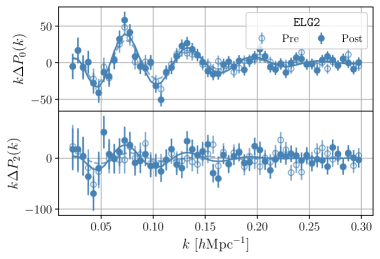
Figure 8: The isolated BAO feature in the monopole and quadrupole before (open circles) and after reconstruction (solid circles) in the power spectrum. The solid and dashsed lines are the best fit BAO models to the unblinded DESI DR1 before (open circles) and after reconstruction (solid circles), respectively. The unit in the y axis $h^{-2}{\rm Mpc}^{2}$ is omitted due to the limited space.

7.1 Reconstructed two-point clustering of DESI DR1

We start with presenting the clustering measurements of the reconstructed catalogs using our default reconstruction method described in Section 4. While we refer to [67] for the full quantitative discussion comparing the mocks and the data, here we note the excellent consistency between the overall clustering amplitude of the Abacus-2 DR1 mocks and that of the data as a function of scale within the fitting ranges pre and post reconstruction, as shown in Figures 5 and 6.

Figures 5 and 6 also compare the pre-reconstruction versus post-reconstruction clustering of DESI DR1 within the fitting ranges. As we adopted the RecSym convention, which preserves the linear RSD boost along the line of sight through the displacement of the random particles, the clustering before and after reconstruction is quite consistent on large scales, as expected. On smaller scales we see in Figure 6 that the post-reconstruction power spectrum is reduced relative to the pre-reconstruction one—this is not unexpected as in general we expect the reconstructed density field to have different nonlinear power due to the coordinate remapping, and there is some analytic evidence for the decrease of power specifically in the case of the post-reconstruction matter power spectrum [106, 17, 154, 155]. From Figure 6, the change in clustering before and after reconstruction of the data (colored solid and dotted lines for monopole and quadrupole, respectively) appears highly consistent with the expectation based on Abacus-2 DR1 mocks within the $1\sigma$ dispersion expected from the RascalC covariance matrice (the black solid and dashed lines with the gray shade for the $1\sigma$ dispersion).

The BAO feature appears moderately sharpened by reconstruction in the LRGs redshift bins, while the improvement is less obvious for other tracers. One can see that the Abacus-2 DR1 mocks replicate the observed level of the BAO sharpening in the DESI DR1 data. Hence, we qualitatively find that the reconstruction of the data is performing as expected given the survey configuration and the reconstruction method we chose. In the next section, where the results of the BAO fits are discussed, we make quantitative comparisons on the aforementioned aspects and show that all tracers had moderate gain from reconstruction at the level consistent with the mocks.

7.2 BAO measurements from the DESI DR1 galaxies

In this section, we present the BAO fitting of all galaxy and quasar tracers using the default fitting method defined in Section 4.3. We focus on the fitting results in configuration space for our discussion below, although we get consistent results in Fourier space Appendix A. All results except for ELG1 and LRG3 will be directly used for the DESI DR1cosmology analysis of [43], with ELG1 and LRG3 incorporated into the analysis via LRG3$+$ELG1. Based on the unblinding tests and the decisions presented in Table 14, we performed two-dimensional BAO fits (${\alpha_{\rm iso}}$ and ${\alpha_{\rm AP}}$) for all tracers other than BGS, ELG1, and QSO. For the latter, we derive ${\alpha_{\rm iso}}$ using only the monopole data.

Table 15, Table 19, Figure 7 and Figure 8 summarize the resulting BAO constraints and visualize the isolated BAO features. Table 15 shows that the $\chi^{2}$ values of the 2-D fits to the correlation functions fall between 33.1 for LRG3$+$ELG1 and 58.6 for ELG2, all for 39 degrees of freedom. The cases of 1-D fits show $\chi^{2}=17.3$ for BGS, $\chi^{2}=20.4$ for ELG1, and $\chi^{2}=32.4$ for QSO for 19 degrees of freedom. The goodness-of-fit is reasonable; the worst cases, ELG2 gives an associated p-value of 2.27% and the QSO gives an associated p-value of 2.82%. Table 19 in appendix summarises the corresponding fits using the power spectrum multiples and shows a reasonable level of the goodness-of-fit with $P(k)$ as well (a smallest p-value of 4.35% for QSO). The BAO measurement scales for the two conjugate spaces are very consistent (less than 0.3% in $\alpha_{\rm iso}$ and $\alpha_{\rm AP}$ except for QSO). This level of consistency between the BAO fits between $\xi(r)$ and $P(k)$ agrees with the Abacus-2 DR1 mocks ([46]).

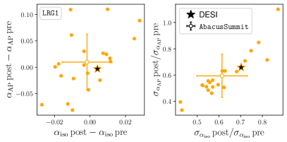
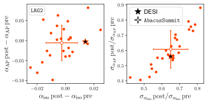
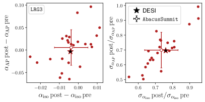
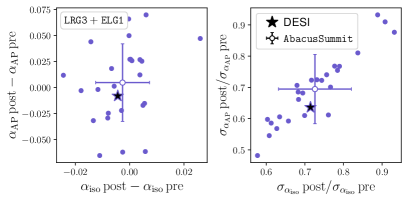
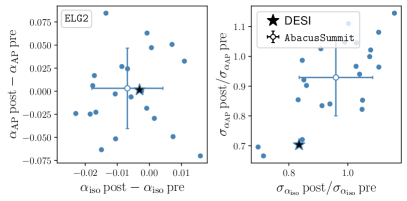
Figure 9: Pre- and post-reconstruction BAO measurements, comparing DESI DR1 measurements (stars) with the 25 Abacus-2 DR1 (the open points with the error bars are the means and the standard deviations around the means of the 25 mocks). Due to the discrepancy between the BAO scales imprinted in the mocks and the BAO scales recovered from the data, we focus on the relative comparison between the pre and the post reconstruction. All DESI DR1 fits are consistent with what is expected from the mocks.

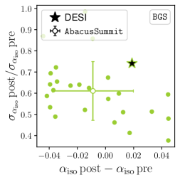
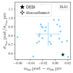
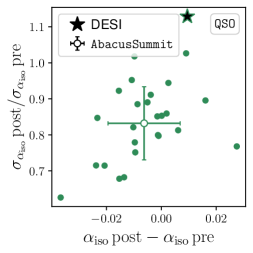
Figure 10: Similar to Figure 9, but showing results for BGS, ELG1, and QSO. The DESI DR1 results are, again, consistent with the range covered by Abacus-2 DR1, except for QSO; the result of QSO shows the reconstruction of DESI DR1 is less efficient than the worst case of the mocks.

Figure 7 displays the BAO features in the correlation function selected for each tracer, compared to the best-fit $\xi$ models for pre-reconstruction (dashed lines) and post-reconstruction data (solid lines). For the 2-D cases, LRG1 shows a distinct BAO feature in the post-reconstruction quadrupole measurement. This is consistent with the $2.29\sigma$ offset of ${\alpha_{\rm AP}}-1$ measured in Table 15. The more the underlying ${\alpha_{\rm AP}}$ differs from the assumed ${\alpha_{\rm AP}}=1$ of the fiducial cosmology, the greater extent to which the feature in the quadrupole would be shifted from that of the monopole and also amplified, as the BAO feature leaks from the monopole to an extent proportional to ${\alpha_{\rm AP}}-1$. This behaviour of the BAO feature in the quadrupole is not evident in the mock data, as the mocks consistently assume ${\alpha_{\rm AP}}=1$ when the they were analyzed. That is, the discrepancy between the BAO signal in the mock and the data merely indicates a measurement of ${\alpha_{\rm AP}}\neq 1$ with $2.29\sigma$ significance. A similar quadrupole feature and the consistent ${\alpha_{\rm AP}}$ best fit is derived from the power spectrum fit.

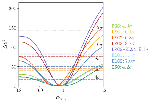
Figure 11: Detection significance of the BAO features in various DESI DR1 galaxy tracers. Solid lines show $\Delta\chi^{2}$ of the BAO fits as a function of $\alpha_{\rm iso}$, i.e., $\chi^{2}$ offset from the minimum $\chi^{2}$. The dashed lines correspond to $\Delta\chi^{2}$ of the noBAO fits, i.e., using a model without the BAO wiggles, after subracting the minimum $\chi^{2}$ of the BAO fit for each tracer. The detection level of the BAO feature for each tracer is shown in the legend.

The reconstruction applied to the QSO sample is less effective than the other tracers due to its high shot noise, as depicted in Figure 7 and detailed in Tables 15 and 19. The mock analysis in [46] suggests $3-8\%$ gain in the precision after reconstruction, though individual realizations will vary considerably due to high shot noise. Additionally, [7] and [138] find that on average the reconstruction will unbias the BAO location, even in this regime of high shot noise. Given these findings, in Table 14, we opted to use the reconstructed QSO result as our fiducial while recognizing its inefficiency from the unblinding test. This decision ensures consistency across cases rather than relying on the realization-dependent performance. In particular, with the future DESI data releases, we anticipate an improved reconstruction performance for the QSO sample, with a reduced fluctuation from realization to realization.

Figures 9 and 10 compare the pre- and post-reconstruction BAO fits for the data and the 25 Abacus-2 DR1 mocks. Due to the discrepancy between the BAO location assumed in the mocks and its measurement in the data, we focus on the changes in the best fits and precision. Except for QSO, the measurements from the data (indicated by stars) lie well within the distribution of the 25 Abacus-2 DR1 mocks, which is the criteria we set as “consistent” given the small number of the mocks. For QSO, the blinded data BAO fit was marginally consistent with the upper boundary (the least effective reconstruction limit) reached by the mocks, therefore passing the unblinding test ([46]). However, the reconstruction of the unblinded DESI DR1 is slightly worse than the blinded case and less efficient than in the worst case of the mocks. We believe that such a slight change before and after unblinding is acceptable.

In detail, we observe the change in the best fit ${\alpha_{\rm iso}}$ with reconstruction is the greatest for LRG2, giving an 1.6% shift ($0.87\sigma$ compared to its pre-reconstruction precision) in $\xi$. In terms of the precision, LRGs show the biggest improvement from reconstruction, a factor of 1.3-1.6 higher precision in $\sigma({\alpha_{\rm iso}})$ and a factor of 1.5-1.8 in $\sigma({\alpha_{\rm AP}})$. For other tracers, we find an improvement of 1.4 for BGS, a factor of 3 for ELG1, and 1.2 ($\alpha_{\rm iso}$) and 1.4 ($\alpha_{\rm AP}$) for ELG2. Reconstruction of these tracers is not as effective as LRGs. In particular, the reconstruction for ELG2 is very likely inhibited due to its low completeness and irregular footprint for DESI DR1. Again, with the future DESI data releases, we anticipate an improved reconstruction performance for the ELGs sample. To summarize, the BAO reconstruction fits lead to a substantial gain for the LRGs, but only a moderate gain for the other tracers.

Figure 11 shows the detection level of the BAO feature. For this plot, one-dimensional BAO fits were performed for all tracers including LRGs and ELG2. Following the standard procedure [156], the fits with the template without the BAO feature were also made (i.e., setting the second term in Eq. 4.1 to zero, hereafter a ‘noBAO fit’). The square root of the difference in $\chi^{2}$ between the pair of the BAO and noBAO fits at the best fit $\alpha_{\rm iso}$ of the former is quoted as the detection significance. The flat likelihood of the noBAO fit is a trivial result of the improved separation between the BAO and noBAO modeling in Eq. 4.1 that the DESI DR1 analysis adopted, i.e., the noBAO modeling now has naturally no dependence on $\alpha_{\rm iso}$, in contrast to previous configuration space analyses (see, e.g., the right-hand panel of figure 12 in [112]). The detection significance, in the increasing order, is 4.0$\sigma$ for BGS, 4.2$\sigma$ for QSO, 6.4$\sigma$ for LRG1, 6.8$\sigma$ for LRG2, 7.0$\sigma$ for ELG2, and 8.7$\sigma$ for LRG3, with the most significant case being $9.1\sigma$ for LRG3+ELG1, closely correlated with the precision.

Tracer	Redshift	Recon	$\alpha_{\rm iso}$	$\alpha_{\rm AP}$	$r_{\rm off}$	$\chi^{2}/{\rm dof}$
BGS	0.1–0.4	Post	$0.9829\pm 0.0185$			17.3/19
LRG1	0.4–0.6	Post	$0.9792\pm 0.0113$	$0.9148\pm 0.0372$	-0.0558	41.8/39
LRG2	0.6–0.8	Post	$0.9661\pm 0.0117$	$1.0459\pm 0.0432$	-0.0514	46.5/39
LRG3	0.8–1.1	Post	$1.0042\pm 0.0090$	$1.0027\pm 0.0299$	-0.0597	46.2/39
LRG3+ELG1	0.8–1.1	Post	$0.9983\pm 0.0081$	$1.0262\pm 0.0278$	-0.1019	33.1/39
ELG1	0.8–1.1	Post	$0.9887\pm 0.0200$			20.4/19
ELG2	1.1–1.6	Post	$0.9876\pm 0.0147$	$0.9904\pm 0.0466$	-0.3031	58.6/39
QSO	0.8–2.1	Post	$1.0015\pm 0.0256$			32.4/19
BGS	0.1–0.4	Pre	$0.9646\pm 0.0258$			14.3/19
LRG1	0.4–0.6	Pre	$0.9760\pm 0.0171$	$0.9258\pm 0.0590$	0.2674	25.8/39
LRG2	0.6–0.8	Pre	$0.9505\pm 0.0191$	$1.0332\pm 0.0769$	0.4130	31.1/39
LRG3	0.8–1.1	Pre	$1.0085\pm 0.0120$	$1.0034\pm 0.0446$	0.2737	48.4/39
LRG3+ELG1	0.8–1.1	Pre	$1.0027\pm 0.0114$	$1.0344\pm 0.0436$	0.2569	53.0/39
ELG1	0.8–1.1	Pre	$0.9404\pm 0.0620$			29.2/19
ELG2	1.1–1.6	Pre	$0.9882\pm 0.0176$	$0.9913\pm 0.0640$	0.0484	42.7/39
QSO	0.8–2.1	Pre	$0.9967\pm 0.0229$			8.1/19

Table 15: Mean values and standard deviations from the marginalized posteriors of the BAO scaling parameters from fits to the unblinded DESI DR1 correlation functions in the $\alpha_{\rm iso}$-$\alpha_{\rm AP}$ basis. These do not include the systematic effect. $r_{\rm off}=C_{\alpha_{\rm iso},\alpha_{\rm AP}}/\sqrt{C_{\alpha_{\rm iso},\alpha_{\rm iso}}C_{\alpha_{\rm AP},\alpha_{\rm AP}}}$.

Tracer	Redshift	Recon	$\alpha_{\parallel}$	$\alpha_{\perp}$	$r_{\rm off}$	$\chi^{2}/{\rm dof}$
LRG1	0.4–0.6	Post	$0.9219\pm 0.0269$	$1.0098\pm 0.0186$	-0.4623	41.8/39
LRG2	0.6–0.8	Post	$0.9955\pm 0.0296$	$0.9527\pm 0.0179$	-0.4386	46.5/39
LRG3	0.8–1.1	Post	$1.0057\pm 0.0214$	$1.0038\pm 0.0139$	-0.4181	46.2/39
LRG3+ELG1	0.8–1.1	Post	$1.0148\pm 0.0193$	$0.9903\pm 0.0126$	-0.4190	33.1/39
ELG2	1.1–1.6	Post	$0.9797\pm 0.0297$	$0.9922\pm 0.0245$	-0.4545	58.6/39
LRG1	0.4–0.6	Pre	$0.9242\pm 0.0485$	$1.0035\pm 0.0243$	-0.4434	25.8/39
LRG2	0.6–0.8	Pre	$0.9766\pm 0.0642$	$0.9402\pm 0.0248$	-0.5015	31.1/39
LRG3	0.8–1.1	Pre	$1.0098\pm 0.0353$	$1.0080\pm 0.0165$	-0.4360	48.4/39
LRG3+ELG1	0.8–1.1	Pre	$1.0230\pm 0.0323$	$0.9930\pm 0.0151$	-0.4549	53.6/39
ELG2	1.1–1.6	Pre	$0.9810\pm 0.0475$	$0.9934\pm 0.0273$	-0.4743	42.7/39

Table 16: Mean values and standard deviations from the marginalized posteriors of the BAO scaling parameters from fits to the unblinded DESI DR1 correlation functions in the $\alpha_{\parallel}$-$\alpha_{\perp}$ basis. These do not include the systematic effect. $r_{\rm off}=C_{\alpha_{\perp},\alpha_{\parallel}}/\sqrt{C_{\alpha_{\perp},\alpha_{\perp}}C_{\alpha_{\parallel},\alpha_{\parallel}}}$.

7.3 BAO constraints projected onto $\alpha_{\perp}$ and $\alpha_{\parallel}$

The parameterisation of the BAO-scale fitting by ${\alpha_{\rm iso}}$ and ${\alpha_{\rm AP}}$ provides a natural separation of the isotropic and anisotropic dilation of the BAO that can be constrained somewhat independently. Table 15 (and Table 19 in Appendix for $P(k)$) displays the cross-correlation coefficients, $r_{\rm off}=C_{\alpha_{\rm iso},\alpha_{\rm AP}}/\sqrt{C_{\alpha_{\rm iso},\alpha_{\rm iso}}C_{\alpha_{\rm AP},\alpha_{\rm AP}}}$. We find the absolute values of $r_{\rm off}$ are less than $\sim 0.10$ for the three LRGs after reconstruction, although it is larger for ELG2($\sim 0.3$). The low value of the cross-correlation allows us to incorporate systematic errors ignoring the covariance between the two dilation parameters, i.e., by adding the statistical covariance from Table 15 with the systematic covariance in Eq. 5.1.

We can also decompose the BAO locations into transverse and line-of-sight dilation parameters $\alpha_{\perp}$ and $\alpha_{\parallel}$ (Eq. 1.1) that are more directly linked to the angular diameter distance and the Hubble parameter at the given redshift. Table 16 (and Table 20 for $P(k)$) shows the BAO constraints from re-fitting $\xi(r)$ into this parameterization rather than transforming them using Eq. 5.2. The cross-correlation coefficients in this case, $r_{\rm off}=C_{\alpha_{\perp},\alpha_{\parallel}}/\sqrt{C_{\alpha_{\perp},\alpha_{\perp}}C_{\alpha_{\parallel},\alpha_{\parallel}}}$, are in excellent agreement with the theoretical Fisher matrix prediction when the BAO feature is singled out [157]. The covariance based on Table 16 will be combined with the covariance for systematics (Eq. 5.4).

7.4 Test of the systematics using the unblinded data

We replicate the tests conducted on the blinded catalogs with the unblinded catalogs to investigate any indications of systematics. Figure 12 illustrates the BAO measurements when comparably optimal variations are introduced around our fiducial setup. The figure compares the baseline fit (using $\xi(r)$) versus the $P(k)$ fit, a different choice of the damping priors, a different choice of the broadband modeling, and a different choice of the reconstruction convention. These are the choices that we consider equally optimal (e.g., the power spectrum fit) or close to being optimal, compared to the default setup. In addition, we also include the pre-reconstruction results (second row).

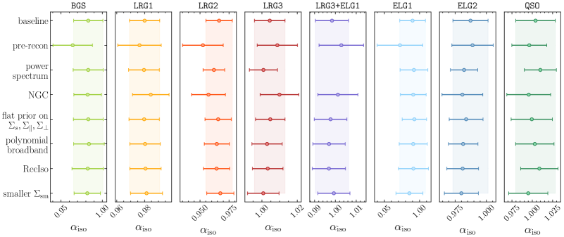
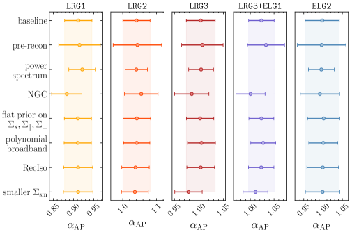
Figure 12: Response of the constraints on the isotropic (top) or anisotropic (bottom) BAO scaling parameters to changes in the data vector or the model assumptions. The baseline configuration adopted for the BAO analysis is shown in the top row, while the remaining rows show single variations around that baseline (see the main text for a description of each case). The consistency between the $\xi(r)$ and $P(k)$ fits and the consistency between the spline broadband versus polynomial broadband are also very high. We identified the Gaussian prior on the sampling parameters as a more robust choice, but even the suboptimal flat priors return very consistent results. The difference between NGC alone and the default (NGC + SGC) shows mild discrepancies for ${\alpha_{\rm AP}}$ of LRG1.

The comparison between the baseline fits versus the fits using $P(k)$ (third whisker) shows high consistency in the derived BAO scales across all cases, as discussed in Section 7.2. The BAO precision from the DESI DR1 $\xi(r)$ fit reasonably agrees with these mock results, especially for ${\alpha_{\rm iso}}$. In some cases, such as LRG2 and ELG2, the $P(k)$-BAO precision tends to be 20-30% better than the $\xi(r)$-BAO error. The Abacus-2 DR1 mock test shows 5-10% larger error with $\xi$; LRG2 lies somewhat beyond the range of the mocks. Thus, opting for the $\xi-BAO$ fits is deemed a conservative choice.

In the fourth whisker, we display the constraints obtained by only fitting data from the NGC, which differs from the baseline case where both galactic caps (NGC+SGC) are combined at the clustering level. In most cases, we only see a small degradation in the parameter constraints compared to the baseline method. The largest deviations appear in ${\alpha_{\rm AP}}$ of LRG1 and LRG3$+$ELG1, but the comparison with mocks shows that this level of deviation can occur for DESI DR1 [46].

The fifth whisker in Figure 12 shows the effect of using a flat, non-informative prior on the BAO non-linear damping parameters. Based on [7], we identified the Gaussian prior on the damping parameters as a more robust choice than a flat prior, but even the sub-optimal, flat priors return very consistent results.

Previous BAO analyses from BOSS [104] and eBOSS [4] adopted a different parameterization for the broadband component of the power spectrum and correlation function, using polynomials with varying degrees of freedom and functional forms. The comparison between our default spline broadband analysis and the polynomial-based broadband method (described in Section 4.3.3) demonstrates excellent consistency (sixth whisker). We note that we have performed this comparison in $\xi(r)$ and have only modified the parameters that capture the broadband component in the modeling, while still integrating all the other theoretical improvements in our analysis.

The second to last whisker shows the constraints using the RecIso convention for reconstruction. This convention, which was the default in previous SDSS BAO analyses [104, 158, 111] supresses higher-order multipoles by removing linear RSD on large scales. To perform this test, we used the (e)BOSS polynomial broadband parametrization for consistency with previous analysis. Overall, we find excellent agreement in the BAO constraints compared to our baseline case using the RecSym convention, in agreement with what was found with mock galaxy catalogs [7] and the blinded DESI data [46].

Finally, in the last row, we show results using a smaller smoothing scale when reconstructing the density field. This corresponds to $10h^{-1}\,{\rm Mpc}$ for BGS, LRGs, and ELGs, and $20h^{-1}\,{\rm Mpc}$ for QSO. We find that the constraints on $\alpha_{\rm iso}$ are only slightly affected by this choice of scale. For ${\alpha_{\rm AP}}$, the largest shift is of $1\sigma$ for LRG3. In [46], tests on the full ensemble of Abacus-2 DR1 show that no statistically significant shifts are observed when comparing these choices of smoothing scales with the baseline. However, variations in individual mocks are expected due to noise fluctuations and are consistent with what is observed in the data.

In summary, the systematic tests conducted directly using unblinded DESI DR1 data demonstrate high consistency across variations of the fiducial setups and data selections (e.g., NGC versus NGC+SGC). Hence, this test bolsters the robustness of our measurements. As a caveat, these consistency tests may not identify systematics that shift all the results together.

7.5 BAO measurements from the combined tracers

There are several redshift ranges in which more than one DESI target class substantially overlaps. Over $0.8<z<1.1$, LRGs, ELGs, and QSO overlap, and over $1.1<z<1.6$, ELGs, and QSO overlap. In particular, over $0.8<z<1.1$, LRG3 and ELG1 are expected to have comparable densities for DESI Y5 and there is a compensatory crossing of the two populations within this redshift range. As both tracers probe the same volume, the two BAO constraints would be highly covariant on large scales, providing a test for consistency in the tracer-independent parameter, such as post-reconstructed BAO locations. Although we have estimated the tracer-dependent systematics on BAO in Section 5.2 within a reasonable (or limited, depending on a view) range of the HODs for each tracer, these overlapping tracers provide an utmost test of the tracer dependence.

When combining the two BAO constraints we must account for this cross-covariance, either using a set of large mocks in which both tracers are present or with an analytical method. Another approach is to construct a combined catalog. A BAO constraint from such a catalog seamlessly combines the information from two BAO measurements from auto-clustering statistics and one from the cross-clustering between ELG1 and LRG3 (hereafter ‘LRG3$\times$ELG1’). The combined catalog, which we defined as LRG3$+$ELG1 in Section 2, may have an additional gain: due to the higher number density, the reconstruction can be more effective. [47] tested the optimal construction of DESI DR1 LRG3 and ELG1. The work includes the test of systematics using auto-clustering measurements and the cross-clustering between the two tracers.

For the unblinded DESI DR1 LRG3$+$ELG1, we find 11% precision-improvement in $\alpha_{\rm iso}$ and 14% improvement in $\alpha_{\rm AP}$ relative to LRG3, as shown in Figure 8 and Table 15. This is highly consistent with the $\sim 10\%$ improvement predicted by [47] based on the mocks.

We find an offset of 0.4% in $\alpha_{\rm iso}$ between LRG3 and LRG3$\times$ELG1 ([47]) and 0.6% between LRG3 versus LRG3$+$ELG1 (Table 15). In $\alpha_{\rm AP}$, we find an offset of 0.4% between LRG3 and LRG3$\times$ELG1 ([47]) and 1.9% between LRG3$+$ELG1 (Table 15). These differences are well within the range covered by the mocks. Therefore, we detect no tracer-dependent bias among the DESI DR1 BAO measurements from LRG3, ELG1, LRG3$\times$ELG1, and LRG3$+$ELG1. With Y3 and Y5, as the completeness of the ELGs increases, we expect a greater improvement from the combined tracer analysis in terms of reconstruction as well as the systematic test. Note that we perform only the $\xi(r)$ fit to the combined tracer, as we have only the RascalC covariance available for the combined tracer.

7.6 Comparison to previous analyses

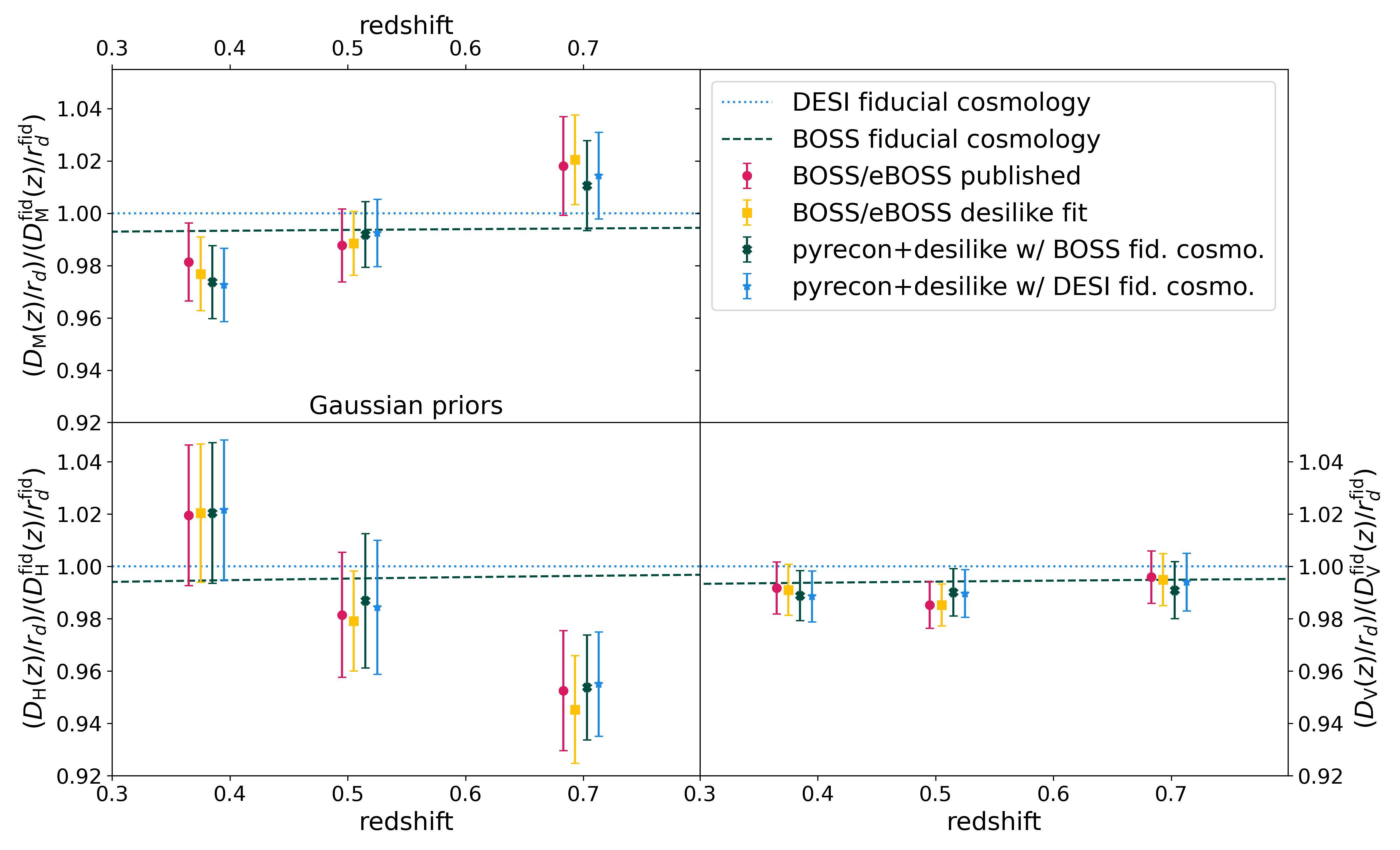
Figure 13: A comparison of the impact of different pipelines on the derived distances, analyzing the published BOSS and eBOSS LRG data. There are three groups of points, one for each of the redshift bins, while the different panels show results for $D_{V}/r_{\mathrm{d}}$, $D_{M}/r_{\mathrm{d}}$, and $D_{H}/r_{\mathrm{d}}$. In each group, the leftmost point is the published BOSS/eBOSS result. The second point from the left uses the published correlation functions and covariance matrices, but refits these using the methodology presented in this paper, while the last two points show the results of reprocessing the BOSS and eBOSS catalogs and randoms through the full DESI pipeline for different fiducial cosmologies. To make the comparison more direct (and to leave the covariance matrices unchanged), we use the RecIso reconstruction scheme here. The fiducial cosmology used to normalize the distance scales on the $y$-axis is the DESI fiducial cosmology used in this paper.

Tracer	$z$	$D_{\rm M}/r_{\rm d}$	$D_{\rm H}/r_{\rm d}$	$r_{\rm off}$
SDSS published
BOSS LOWZ+CMASS	0.2 - 0.5	$10.23\pm 0.17$	$25.00\pm 0.76$	-0.39
BOSS LOWZ+CMASS	0.4 - 0.6	$13.36\pm 0.21$	$22.33\pm 0.58$	-0.39
eBOSS LRG	0.6 - 1.0	$17.86\pm 0.33$	$19.33\pm 0.53$	-0.33
SDSS published/desilike refit
BOSS LOWZ+CMASS	0.2 - 0.5	$10.18\pm 0.15$	$25.1\pm 0.65$	-0.425
BOSS LOWZ+CMASS	0.4 - 0.6	$13.35\pm 0.17$	$22.27\pm 0.43$	-0.404
eBOSS LRG	0.6 - 1.0	$17.9\pm 0.3$	$19.16\pm 0.42$	-0.416
DESI pipeline
BOSS LOWZ+CMASS	0.2 - 0.5	$10.15\pm 0.15$	$25.10\pm 0.66$	-0.45
BOSS LOWZ+CMASS	0.4 - 0.6	$13.39\pm 0.17$	$22.44\pm 0.58$	-0.43
eBOSS LRG	0.6 - 1.0	$17.72\pm 0.30$	$19.33\pm 0.41$	-0.40

Table 17: Comparison between the SDSS published results and the reanalysis using the DESI pipeline. Among several options we tested in Section 7.6, we present the DESI reanalysis with IFFT RecIso under the BOSS fiducial cosmology, to best match the clustering amplitude assumed in the published covariance matrices. We did not add the SDSS systematic errors in the middle group. We also did not add the DESI systematic errors from Eq. 5.4 to the bottom group, but the difference is negligible.

Given the changes described above in our pipeline, we revisit the SDSS (BOSS and eBOSS) data previously analyzed to quantify the impact of these changes on previously published results [159]. We do so in two stages. First, we refit the published correlation functions (using the published covariance matrices) to measure the distance scale. Second, we rerun the reconstruction pipeline using our new convention and then re-fit the updated correlation functions. Figure 13 shows the results of these comparisons for the three redshift bins used in the SDSS ([159]).

The red point of each group in Figure 13 (first from the left) is the published BOSS/eBOSS result for $\alpha$, while the yellow point (second from the left) uses the published correlation functions and covariance matrices, but refits these using the baseline methodology described in this paper. For the fits performed here, we use damping parameters with Gaussian priors to match this analysis, while the published analyses used a fixed damping scale. The differences between these points are due to two primary factors. The first are changes in how the BAO features are damped. When computing the theoretical correlation functions in the previous analyses, the power spectrum was damped by an additional smoothing of $1h^{-1}\,{\rm Mpc}$ to accelerate the convergence of the Hankel transform and reduce ringing. This effectively changes the damping scales. Furthermore, previous analyses applied the small-scale streaming velocities to both the BAO and the broadband shape, while our current analysis only applies it to the broadband shape (Section 4.3.4). Additionally, the current analysis has a new separation of the BAO and broadband shape. The top and middle group of Table 17 shows the net change from all of these effects.

We also explore the effect of different reconstruction conventions using the full DESI pipeline and setup. We reprocess the BOSS and eBOSS catalogs and randoms using pyrecon and pycorr under cosmodesi and fit using the fiducial setup of Section 4.3 implemented in desilike. The two rightmost points in each group of Figure 13 show the results of this reprocessing, and the bottom group of Table 17 shows their impact. When comparing these numbers, we emphasize that the exact details of how the data sets are assigned to grids and padded will also affect the derived displacement fields. These different implementations should be thought of as yielding different data sets, even though they are derived from the same initial sets of galaxy positions. Given that the remaining differences are well within the statistical precision of these samples, we therefore conclude that our new analysis does yield consistent results with published results. The companion cosmological interpretation paper [43] will present a detailed consistency check at the level of the underlying cosmological parameters.

8 The final distance measurements and the Hubble Diagram

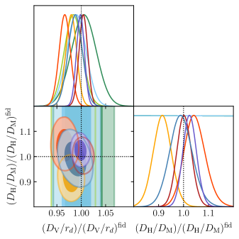
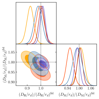
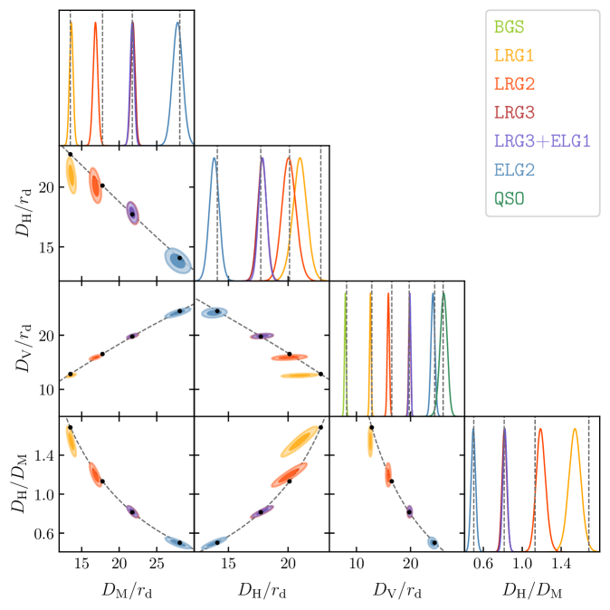
Figure 14: The final BAO-only distance posteriors, shown as measurements of $D_{\mathrm{M}}/r_{\mathrm{d}}$, $D_{\mathrm{H}}/r_{\mathrm{d}}$, $D_{\mathrm{V}}/r_{\mathrm{d}}$, and $D_{\mathrm{H}}/D_{\mathrm{M}}$, compared against the fiducial Planck 2018-$\Lambda$CDM distances. In the bottom panel, the prediction at the effective redshift of each sample is shown by the black dots along the dashed lines: $z_{\rm eff}=0.51$ (LRG1), 0.71 (LRG2), 0.93 (LRG3), and 1.32 (ELG2). The uncertainty intervals on the plot do not take account of the systematic errors but doing so would make little visible difference.

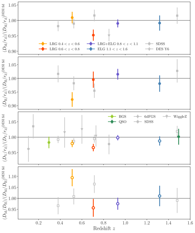
Figure 15: Hubble diagram of the BAO distance scales measured from the unblinded galaxy and quasar data, compared to those from earlier BAO measurements by the 6 degree Field Galaxy Survey (6dFGS, [27]), WiggleZ [103], the Sloan Digital Sky Survey (SDSS, [159]), and the Dark Energy Survey (DES Y6, [160]), as labelled. From top to bottom, the panels show $D_{\mathrm{M}}/r_{\mathrm{d}}$, $D_{\mathrm{H}}/r_{\mathrm{d}}$, $D_{\mathrm{V}}/r_{\mathrm{d}}$ and $D_{\mathrm{M}}/D_{\mathrm{H}}$, all relative to the respective quantities evaluated in the DESI fiducial cosmology described in Section 1. For 6dFGS, WiggleZ and some redshift bins of SDSS and DESI, only $D_{\mathrm{V}}/r_{\mathrm{d}}$ measurements were possible due to the low signal-to-noise ratio, so these points are only shown in the third panel. For the DESI and SDSS redshift bins where both $D_{\mathrm{M}}/r_{\mathrm{d}}$ and $D_{\mathrm{H}}/r_{\mathrm{d}}$ were measured, results for $D_{\mathrm{V}}/r_{\mathrm{d}}$ and $D_{\mathrm{M}}/D_{\mathrm{H}}$ in the third and fourth panels are displayed with open markers to indicate the repetition of information in the top two panels in a different parametrisation. Note that a slight offset has been applied to the effective redshifts of the SDSS results at $z_{\rm eff}=0.51$ and $0.70$ to avoid overlap and ensure visibility in this figure.

In this section, we present our final distance measurements, construct the Hubble diagram, compare with the previous BAO measurements, and discuss any implications. We adopt the configuration space measurements as our fiducial results.

Tracer	$z_{\rm eff}$	$D_{\rm M}/r_{\rm d}$	$D_{\rm H}/r_{\rm d}$	$D_{\rm V}/r_{\rm d}$	$D_{\rm H}/D_{\rm M}$	$r_{\rm off}$
BGS	0.30	—	—	$7.93\pm 0.15$	—	—
LRG1	0.51	$13.62\pm 0.25$	$20.98\pm 0.61$	$12.56\pm 0.15$	$1.542\pm 0.063$	$-0.445$
LRG2	0.71	$16.85\pm 0.32$	$20.08\pm 0.60$	$15.90\pm 0.20$	$1.193\pm 0.049$	$-0.420$
LRG3	0.92	$21.81\pm 0.31$	$17.83\pm 0.38$	$19.82\pm 0.18$	$0.818\pm 0.025$	$-0.393$
LRG3+ELG1	0.93	$21.71\pm 0.28$	$17.88\pm 0.35$	$19.86\pm 0.17$	$0.824\pm 0.022$	$-0.389$
ELG1	0.95	—	—	$20.01\pm 0.41$	—	—
ELG2	1.32	$27.79\pm 0.69$	$13.82\pm 0.42$	$24.13\pm 0.36$	$0.498\pm 0.023$	$-0.444$
QSO	1.49	—	—	$26.07\pm 0.67$	—	—

Table 18: Final summary of the derived BAO distance scales from fits to the post-reconstruction correlation function multipoles for each DESI target sample, including the systematics from Eqs. 5.1 and 5.4. We display results in terms of the mean values and standard deviations from the marginalized posteriors of each parameter. $r_{\rm off}$ is the correlation coefficient between $D_{\rm M}/r_{\rm d}$ and $D_{\rm H}/r_{\rm d}$. The results in this table are used for the cosmology analysis in [43].

8.1 The final distance measurements with systematics

In Table 18, we combine the best-fit BAO measurements, based on Tables 15 and 16, with the total systematic error budget from Eqs. 5.1 and 5.4, and present the final distance posteriors to be used for cosmology inference in [43]. With the knowledge of the fiducial distance-to-redshift relation and the sound horizon scale used in the analysis, we can convert the BAO measurements to the distance observables: comoving angular diameter distance $D_{M}(z)$,

$$\frac{D_{M}(z)}{r_{\mathrm{d}}}\equiv\frac{D_{A}(z)[1+z]}{r_{\mathrm{d}}}=\alpha_{\perp}\frac{D^{\rm fid}_{M}(z)}{r^{\rm fid}_{d}},$$ (8.1)

the Hubble distance $D_{H}(z)$,

$$\frac{D_{H}(z)}{r_{\mathrm{d}}}\equiv\frac{c}{H(z)r_{\mathrm{d}}}=\alpha_{\parallel}\frac{D^{\rm fid}_{H}(z)}{r^{\rm fid}_{d}},$$ (8.2)

and the spherically-averaged distance $D_{V}(z)$,

$$\frac{D_{V}(z)}{r_{\mathrm{d}}}\equiv\frac{[zD^{2}_{M}(z)D_{H}(z)]^{1/3}}{r_{\mathrm{d}}}=\alpha_{\rm iso}\frac{D^{\rm fid}_{V}(z)}{r^{\rm fid}_{d}}.$$ (8.3)

Figure 14 graphically presents our distance constraints of all tracers relative to the fiducial Planck 2018-$\Lambda$CDM distances. The plot shows offsets from the Planck 2018-$\Lambda$CDM predictions for $0.4<z<0.6$ (${\tt LRG1}\ (z_{\rm eff}=0.51)$) and $0.6<z<0.8$. The deviation at ${\tt LRG1}\ (z_{\rm eff}=0.51)$ is mainly for $D_{H}/r_{\mathrm{d}}$. This means that the line-of-sight BAO scale appears bigger than the transverse BAO scale, when the observed space is mapped to the physical space using the metric of the Planck 2018-$\Lambda$CDM cosmology.

On the other hand, the deviation at ${\tt LRG2}\ (z_{\rm eff}=0.71)$ is mainly in $D_{V}/r_{\mathrm{d}}$ in $D_{M}/r_{\mathrm{d}}$. That is, the transverse BAO scale at this redshift appears much larger than the prediction of the Planck 2018-$\Lambda$CDM, giving a smaller $D_{\mathrm{V}}/r_{\mathrm{d}}$ and $D_{\mathrm{M}}/r_{\mathrm{d}}$ at this redshift. The cosmological implication of these deviations is extensively tested in [43]. At $z>0.8$, our BAO measurements are consistent with the expansion history predicted by the Planck 2018-$\Lambda$CDM.

We then construct a Hubble diagram using DESI DR1 BAO-only distance measurements and also with previous spectroscopic BAO measurements overlaid (Figure 15). Again, we defer the thorough investigation of the cosmological implications of these measurements in combination with the DESI DR1 Ly-$\alpha$ BAO measurement ([42]) to [43].

8.2 Remarks on the discrepancy between SDSS and DESI over $0.6<z<0.8$

Figure 15 shows noticeable discrepancy between the DESI DR1 measurement at $z_{\rm eff}=0.71$ (LRG2) and SDSS LRG (eBOSS DR16) at $z_{\rm eff}=0.7$ ($0.6<z<0.85$). SDSS LRG measured $D_{M}(0.70)/r_{\mathrm{d}}=17.86\pm 0.33$ and $D_{H}(0.80)/r_{\mathrm{d}}=19.33\pm 0.53$, with $r_{\rm off}=-0.32$ [111], while this paper reports $D_{M}(0.71)/r_{\mathrm{d}}=16.85\pm 0.32$, $D_{H}(0.71)/r_{\mathrm{d}}=20.08\pm 0.60$ with $r_{\rm off}=-0.420$ for LRG2.

An approximate estimate of the cross-correlation between the two tracers in the power spectrum space is 0.21. Assuming that this directly propagates to the cross-correlation of the BAO measurements, the discrepancy is close to $\sim$3$\sigma$ for $D_{M}/r_{\mathrm{d}}$ and $D_{V}/r_{\mathrm{d}}$ when we account for the difference between $z_{\rm eff}=0.7$ and $z_{\rm eff}=0.71$ using the Planck 2018-$\Lambda$CDM cosmology.

An insight gleaned from Section 7.6 and numerous robustness tests conducted in this paper is that an estimator derived from a particular dataset undergoing different pipelines can be regarded as two distinct yet unbiased estimators of the truth, provided each is individually demonstrated to be unbiased. Hence, the cross-correlation coefficient could be much lower than the theoretical estimate, suggesting that the observed 3$\sigma$ discrepancy between SDSS and DESI is likely an upper limit. However, the lower limit, determined assuming no correlation, is still 2.7$\sigma$. The DESI reanalysis in Table 17 yields a slightly lower BAO measurement compared to the published SDSS measurements, resulting in significances of 2.8$\sigma$ and 2.5$\sigma$, assuming cross-correlations of 0.21 and 0, respectively.

While this 2.5$\sigma$–3$\sigma$ discrepancy warrants attention, we have not identified any sources of non-statistical discrepancy from both sets of the data. We reiterate the significant value of a blinded analysis of DESI DR1, conducted and unblinded without being affected by prior knowledge of any discrepancies compared to previous measurements. We anticipate gaining a deeper understanding of its nature through the analysis of DESI Y3 and Y5 data.

9 Conclusion

In this paper, we presented the first BAO scale measurements from the DESI galaxies and quasars since the start of its data collection in 2021. The measurements from DESI DR1 include over 5.7 million galaxy and quasar redshifts over the redshift range of $0.1<z<2.1$, with the total effective survey volume of $\sim 18\ \text{Gpc}^{3}$. This marks the largest volume and the most redshifts used for any spectroscopic BAO measurements. We summarize the final distance constraints for six redshift bins, detailed in Table 18, as:

• Distance precision (i.e., $D_{\mathrm{V}}/r_{\mathrm{d}}$) ranges of 1.9% (BGS at $z_{\rm eff}=0.3$), 1.2% (LRG1 at $z_{\rm eff}=0.51$), 1.2% (LRG2 at $z_{\rm eff}=0.71$), 0.8% (LRG3$+$ELG1 at $z_{\rm eff}\sim 0.95$), 1.5% (ELG2 at $z_{\rm eff}=1.32$), and 2.6% (QSO at $z_{\rm eff}=1.49$). The aggregate precision of all measurements is 0.52% on the BAO scale.

• The anisotropic distortion of the BAO (i.e., $D_{\mathrm{H}}/D_{\mathrm{M}}$) is measured with the precision of 4.1% (LRG1), 4.1% (LRG2), 2.7% (LRG3$+$ELG1), and 4.6% (QSO).

Our measurement marks the highest precision on the cosmological distances for $z>0.8$, compared to the previous survey, and also collectively marks the highest aggregate precision. Comparing this with the SDSS BAO measurements ([159, 161]), which report an aggregate precision of 0.64% on $D_{V}/r_{\mathrm{d}}$ for all galaxy and quasar tracers combined, the aggregate precision of DESI DR1 in this paper returns 0.52%. The detection levels range from the highest 9.1$\sigma$ for LRG3$+$ELG1 to the lowest 4.0$\sigma$ for BGS. We produced the first high-significance BAO detection using galaxies $z>1$, i.e., ELG2 at the significance of 7.0$\sigma$. Proving the robust nature of the BAO for ELGs, despite its substantial imaging systematics, is an important result for upcoming Stage-V BAO surveys.

Alongside the state-of-the-art dataset, the DESI DR1 BAO analysis incorporated several significant novel elements. Our analysis is one of the first to rigorously implement blinding in the BAO analysis (c.f. [160]) and the first catalog-level blinded BAO analysis (Section 2.3). This approach was adopted to mitigate confirmation bias. The true clustering was unveiled only once the blinded catalogs successfully passed a series of unblinding tests (refer to Table 14). Anticipating the unprecedented precision of DESI BAO beyond DESI DR1, our analysis incorporated physically motivated enhancements to the BAO fitting and reconstruction methods from previous surveys. This included the adoption of a new reconstruction method (Section 4.2) and improved treatment for separating BAO from broadband signals (Section 4.3). We introduced a spline-based broadband model to reduce parameterization dependence on data signal-to-noise. We constructed and analyzed a combined tracer catalog for LRGs and ELGs spanning $0.8<z<1.1$, merging information from both tracers and facilitating an additional systematic test (refer to Section 7.5). This approach yielded an improvement of approximately 10%, with even greater improvements anticipated for future DESI analyses.

We employed a unified BAO analysis pipeline and methodology across all galaxy and quasar tracers, as well as between configuration space and Fourier space, marking a first in BAO surveys. The algorithms utilized in this study are incorporated into a publicly accessible repository developed by the collaboration, with some currently available and others planned for future release. We meticulously coordinated a systematic study across all tracers and components. Our investigation covered theoretical modeling effects (Section 4.4), tracer-specific systematics (Section 5.2), assumptions regarding fiducial cosmology (Section 5.4), observational systemtaics (Section 5.3), reconstruction algorithm choices (Section 4.2), and covariance matrix choice (Section 4.5). Summary of these findings is provided in Table 13, yielding conservative systematics estimates of 0.245% for the isotropic BAO scale and 0.300% for the anisotropic distortion of the BAO feature (i.e., the Alcock-Paczynski effect). Further details are available in supporting papers listed in Table 1.

To quantify the impact of the changes we made in the DESI pipeline, we revisited the SDSS BAO measurements using the DESI pipelines. We conclude that the two measurement pipelines yield sufficiently similar results for these datasets (refer to Section 7.6), although we anticipate that the new method will be advantageous for the higher-precision dataset expected in the future.

From the Hubble diagram constructed from our results, we found that our BAO measurements indicate systematically larger observed BAO scales than the prediction of Planck 2018-$\Lambda$CDM at $z<0.8$, and therefore lower distances. For $z_{\rm eff}=0.51$, this discrepancy is sourced from the line-of-sight BAO: it appears bigger than the transverse BAO scale, when the observed space is mapped to the physical space using the metric of the Planck 2018-$\Lambda$CDM cosmology. For $z_{\rm eff}=0.71$, the discrepancy is sourced from the overall size of the BAO (and more transverse than the line-of-sight). The transverse BAO scale at this redshift appears much larger than the prediction of the Planck 2018-$\Lambda$CDM, implying a smaller $D_{\mathrm{V}}/r_{\mathrm{d}}$ and $D_{\mathrm{M}}/r_{\mathrm{d}}$ at this redshift. Accordingly, we found a large discrepancy between the DESI BAO measurement at $z_{\rm eff}=0.71$ and the SDSS measurement at $z_{\rm eff}=0.7$. The level of discrepancy is $\sim$3$\sigma$ on $D_{\mathrm{M}}/r_{\mathrm{d}}$. At $z>0.8$, our BAO measurements are consistent with that of the Planck 2018-$\Lambda$CDM. We emphasize the value of our blinded analysis in achieving the DESI DR1 BAO measurements without prior knowledge of comparisons with previous measurements. An extensive investigation on the cosmological implication of these discrepancies from Planck 2018-$\Lambda$CDM, in combination with the BAO measurement from the Lyman-$\alpha$ forest ([42]), is presented in the DESI DR1 cosmology paper, [43].

Assuming the same sample definitions (which are conservative for DESI DR1), the final DESI dataset will be more than a factor of 3 in terms of the effective volume (4-5 for ELGs, $\sim 3$ for LRGs, and 2-3 for BGS and QSO) compared to DESI DR1, using more than 20 million unique redshifts. Through the analysis of the DESI Y3 and Y5 data, we anticipate to gain a deeper understanding of the nature of the intriguing measurements we observed.

10 Data Availability

The data used in this analysis will be made public along the Data Release 1 (details in https://data.desi.lbl.gov/doc/releases/).

Appendix A BAO measurements in Fourier space

Tracer	Redshift	Recon	$\alpha_{\rm iso}$	$\alpha_{\rm AP}$	$r_{\rm off}$	$\chi^{2}/{\rm dof}$
BGS	0.1–0.4	Post	$0.9848\pm 0.0242$			27.4/41
LRG1	0.4–0.6	Post	$0.9799\pm 0.0118$	$0.9231\pm 0.0371$	-0.1413	85.9/87
LRG2	0.6–0.8	Post	$0.9624\pm 0.0098$	$1.0431\pm 0.0356$	-0.0373	82.1/87
LRG3	0.8–1.1	Post	$1.0005\pm 0.0081$	$1.0057\pm 0.0261$	-0.0991	100.8/87
ELG1	0.8–1.1	Post	$0.9913\pm 0.0249$			47.6/41
ELG2	1.1–1.6	Post	$0.9827\pm 0.0112$	$0.9986\pm 0.0352$	-0.2217	103.8/87
QSO	0.8–2.1	Post	$1.0094\pm 0.0212$			57.7/41
BGS	0.1–0.4	Pre	$0.9657\pm 0.0364$			50.0/41
LRG1	0.4–0.6	Pre	$0.9774\pm 0.0179$	$0.9316\pm 0.0595$	0.2927	87.1/87
LRG2	0.6–0.8	Pre	$0.9487\pm 0.0148$	$1.0324\pm 0.0610$	0.4315	87.5/87
LRG3	0.8–1.1	Pre	$1.0022\pm 0.0107$	$1.0132\pm 0.0387$	0.2259	108.0/87
ELG1	0.8–1.1	Pre	$0.9819\pm 0.0619$			51.2/41
ELG2	1.1–1.6	Pre	$0.9873\pm 0.0152$	$1.0191\pm 0.0558$	0.1395	95.6/87
QSO	0.8–2.1	Pre	$1.0006\pm 0.0206$			49.3/41

Table 19: Mean values and standard deviations from the marginalized posteriors of the BAO scaling parameters from fits to the unblinded DESI DR1 power spectra in the $\alpha_{\rm iso}$-$\alpha_{\rm AP}$ basis. Systematic effects are not included. The $P(k)$ fits do not include LRG3$+$ELG1, as we do not have a covariance available for the combined tracer in $P(k)$. $r_{\rm off}=C_{\alpha_{\rm iso},\alpha_{\rm AP}}/\sqrt{C_{\alpha_{\rm iso},\alpha_{\rm iso}}C_{\alpha_{\rm AP},\alpha_{\rm AP}}}$.

Tracer	Redshift	Recon	$\alpha_{\parallel}$	$\alpha_{\perp}$	$r_{\rm off}$	$\chi^{2}/{\rm dof}$
LRG1	0.4-0.6	Post	$0.928\pm 0.023$	$1.007\pm 0.018$	-0.429	85.9/87
LRG2	0.6-0.8	Post	$0.987\pm 0.022$	$0.949\pm 0.014$	-0.419	82.1/87
LRG3	0.8-1.1	Post	$1.004\pm 0.018$	$0.999\pm 0.012$	-0.401	100.8/87
ELG2	1.1-1.6	Post	$0.979\pm 0.022$	$0.984\pm 0.018$	-0.416	103.8/87
LRG1	0.4-0.6	Pre	$0.924\pm 0.040$	$1.003\pm 0.021$	-0.399	87.1/87
LRG2	0.6-0.8	Pre	$0.975\pm 0.044$	$0.937\pm 0.017$	-0.440	87.5/87
LRG3	0.8-1.1	Pre	$1.012\pm 0.029$	$0.997\pm 0.014$	-0.406	108.0/87
ELG2	1.1-1.6	Pre	$1.004\pm 0.041$	$0.979\pm 0.020$	-0.419	95.6/87

Table 20: Mean values and standard deviations from the marginalized posteriors of the BAO scaling parameters from fits to the unblinded DESI DR1 power spectra in the $\alpha_{\parallel}$-$\alpha_{\perp}$ basis. Systematic effects are not included. $r_{\rm off}=C_{\alpha_{\perp},\alpha_{\parallel}}/\sqrt{C_{\alpha_{\perp},\alpha_{\perp}}C_{\alpha_{\parallel},\alpha_{\parallel}}}$.

Tables 19 and 20 shows the BAO measurements using the power spectrum measurements that should be directly compared with the measurements in Tables 15 and 16. As noted in the main section, our analytical and mock-based covariances have not fully converged in our Fourier space analysis, thus we consider the power spectrum results less robust. Nevertheless, the power spectrum results serve as a consistency check of our results based on the correlation function as the two are in good agreement, in line with expectations derived from mock tests.

Appendix B Author Affiliations

¹Instituto de Física Teórica (IFT) UAM/CSIC, Universidad Autónoma de Madrid, Cantoblanco, E-28049, Madrid, Spain

²Lawrence Berkeley National Laboratory, 1 Cyclotron Road, Berkeley, CA 94720, USA

³Physics Dept., Boston University, 590 Commonwealth Avenue, Boston, MA 02215, USA

⁴Tata Institute of Fundamental Research, Homi Bhabha Road, Mumbai 400005, India

⁵Centre for Extragalactic Astronomy, Department of Physics, Durham University, South Road, Durham, DH1 3LE, UK

⁶Institute for Computational Cosmology, Department of Physics, Durham University, South Road, Durham DH1 3LE, UK

⁷Department of Physics, University of Michigan, Ann Arbor, MI 48109, USA

⁸Leinweber Center for Theoretical Physics, University of Michigan, 450 Church Street, Ann Arbor, Michigan 48109-1040, USA

⁹IRFU, CEA, Université Paris-Saclay, F-91191 Gif-sur-Yvette, France

¹⁰Institut de Física d’Altes Energies (IFAE), The Barcelona Institute of Science and Technology, Campus UAB, 08193 Bellaterra Barcelona, Spain

¹¹Instituto Avanzado de Cosmología A. C., San Marcos 11 - Atenas 202. Magdalena Contreras, 10720. Ciudad de México, México

¹²Instituto de Ciencias Físicas, Universidad Autónoma de México, Cuernavaca, Morelos, 62210, (México)

¹³Physics Department, Yale University, P.O. Box 208120, New Haven, CT 06511, USA

¹⁴Department of Physics and Astronomy, University of California, Irvine, 92697, USA

¹⁵Department of Physics, Kansas State University, 116 Cardwell Hall, Manhattan, KS 66506, USA

¹⁶Department of Physics & Astronomy, University of Rochester, 206 Bausch and Lomb Hall, P.O. Box 270171, Rochester, NY 14627-0171, USA

¹⁷Institute for Astronomy, University of Edinburgh, Royal Observatory, Blackford Hill, Edinburgh EH9 3HJ, UK

¹⁸Dipartimento di Fisica “Aldo Pontremoli”, Università degli Studi di Milano, Via Celoria 16, I-20133 Milano, Italy

¹⁹Centre for Astrophysics & Supercomputing, Swinburne University of Technology, P.O. Box 218, Hawthorn, VIC 3122, Australia

²⁰NSF NOIRLab, 950 N. Cherry Ave., Tucson, AZ 85719, USA

²¹Department of Physics and Astronomy, The University of Utah, 115 South 1400 East, Salt Lake City, UT 84112, USA

²²Department of Physics & Astronomy, University College London, Gower Street, London, WC1E 6BT, UK

²³Department of Astronomy and Astrophysics, University of Chicago, 5640 South Ellis Avenue, Chicago, IL 60637, USA

²⁴Fermi National Accelerator Laboratory, PO Box 500, Batavia, IL 60510, USA

²⁵Korea Astronomy and Space Science Institute, 776, Daedeokdae-ro, Yuseong-gu, Daejeon 34055, Republic of Korea

²⁶Institute of Cosmology and Gravitation, University of Portsmouth, Dennis Sciama Building, Portsmouth, PO1 3FX, UK

²⁷Departamento de Astrofísica, Universidad de La Laguna (ULL), E-38206, La Laguna, Tenerife, Spain

²⁸Instituto de Astrofísica de Canarias, C/ Vía Láctea, s/n, E-38205 La Laguna, Tenerife, Spain

²⁹Department of Physics and Astronomy, University of Sussex, Brighton BN1 9QH, U.K

³⁰Departamento de Física, Instituto Nacional de Investigaciones Nucleares, Carreterra México-Toluca S/N, La Marquesa, Ocoyoacac, Edo. de México C.P. 52750, México

³¹Institute for Advanced Study, 1 Einstein Drive, Princeton, NJ 08540, USA

³²Center for Cosmology and AstroParticle Physics, The Ohio State University, 191 West Woodruff Avenue, Columbus, OH 43210, USA

³³NASA Einstein Fellow

³⁴School of Mathematics and Physics, University of Queensland, 4072, Australia

³⁵Instituto de Física, Universidad Nacional Autónoma de México, Cd. de México C.P. 04510, México

³⁶CIEMAT, Avenida Complutense 40, E-28040 Madrid, Spain

³⁷Department of Physics & Astronomy and Pittsburgh Particle Physics, Astrophysics, and Cosmology Center (PITT PACC), University of Pittsburgh, 3941 O’Hara Street, Pittsburgh, PA 15260, USA

³⁸Department of Astronomy, School of Physics and Astronomy, Shanghai Jiao Tong University, Shanghai 200240, China

³⁹Space Sciences Laboratory, University of California, Berkeley, 7 Gauss Way, Berkeley, CA 94720, USA

⁴⁰University of California, Berkeley, 110 Sproul Hall #5800 Berkeley, CA 94720, USA

⁴¹Universities Space Research Association, NASA Ames Research Centre

⁴²Center for Astrophysics $|$ Harvard & Smithsonian, 60 Garden Street, Cambridge, MA 02138, USA

⁴³Department of Physics, The Ohio State University, 191 West Woodruff Avenue, Columbus, OH 43210, USA

⁴⁴The Ohio State University, Columbus, 43210 OH, USA

⁴⁵Kavli Institute for Particle Astrophysics and Cosmology, Stanford University, Menlo Park, CA 94305, USA

⁴⁶SLAC National Accelerator Laboratory, Menlo Park, CA 94305, USA

⁴⁷Instituto de Astrofísica de Andalucía (CSIC), Glorieta de la Astronomía, s/n, E-18008 Granada, Spain

⁴⁸Ecole Polytechnique Fédérale de Lausanne, CH-1015 Lausanne, Switzerland

⁴⁹Departamento de Física, Universidad de los Andes, Cra. 1 No. 18A-10, Edificio Ip, CP 111711, Bogotá, Colombia

⁵⁰Observatorio Astronómico, Universidad de los Andes, Cra. 1 No. 18A-10, Edificio H, CP 111711 Bogotá, Colombia

⁵¹Department of Physics, The University of Texas at Dallas, Richardson, TX 75080, USA

⁵²Institut d’Estudis Espacials de Catalunya (IEEC), 08034 Barcelona, Spain

⁵³Institute of Space Sciences, ICE-CSIC, Campus UAB, Carrer de Can Magrans s/n, 08913 Bellaterra, Barcelona, Spain

⁵⁴Departament de Física Quàntica i Astrofísica, Universitat de Barcelona, Martí i Franquès 1, E08028 Barcelona, Spain

⁵⁵Institut de Ciències del Cosmos (ICCUB), Universitat de Barcelona (UB), c. Martí i Franquès, 1, 08028 Barcelona, Spain.

⁵⁶Consejo Nacional de Ciencia y Tecnología, Av. Insurgentes Sur 1582. Colonia Crédito Constructor, Del. Benito Juárez C.P. 03940, México D.F. México

⁵⁷Departamento de Física, Universidad de Guanajuato - DCI, C.P. 37150, Leon, Guanajuato, México

⁵⁸Centro de Investigación Avanzada en Física Fundamental (CIAFF), Facultad de Ciencias, Universidad Autónoma de Madrid, ES-28049 Madrid, Spain

⁵⁹Excellence Cluster ORIGINS, Boltzmannstrasse 2, D-85748 Garching, Germany

⁶⁰University Observatory, Faculty of Physics, Ludwig-Maximilians-Universität, Scheinerstr. 1, 81677 München, Germany

⁶¹Department of Astrophysical Sciences, Princeton University, Princeton NJ 08544, USA

⁶²Kavli Institute for Cosmology, University of Cambridge, Madingley Road, Cambridge CB3 0HA, UK

⁶³Department of Astronomy, The Ohio State University, 4055 McPherson Laboratory, 140 W 18th Avenue, Columbus, OH 43210, USA

⁶⁴Department of Physics, Southern Methodist University, 3215 Daniel Avenue, Dallas, TX 75275, USA

⁶⁵Department of Physics and Astronomy, University of Waterloo, 200 University Ave W, Waterloo, ON N2L 3G1, Canada

⁶⁶Perimeter Institute for Theoretical Physics, 31 Caroline St. North, Waterloo, ON N2L 2Y5, Canada

⁶⁷Waterloo Centre for Astrophysics, University of Waterloo, 200 University Ave W, Waterloo, ON N2L 3G1, Canada

⁶⁸Graduate Institute of Astrophysics and Department of Physics, National Taiwan University, No. 1, Sec. 4, Roosevelt Rd., Taipei 10617, Taiwan

⁶⁹Sorbonne Université, CNRS/IN2P3, Laboratoire de Physique Nucléaire et de Hautes Energies (LPNHE), FR-75005 Paris, France

⁷⁰Department of Astronomy and Astrophysics, UCO/Lick Observatory, University of California, 1156 High Street, Santa Cruz, CA 95064, USA

⁷¹Department of Astronomy and Astrophysics, University of California, Santa Cruz, 1156 High Street, Santa Cruz, CA 95065, USA

⁷²Department of Astronomy & Astrophysics, University of Toronto, Toronto, ON M5S 3H4, Canada

⁷³University of Science and Technology, 217 Gajeong-ro, Yuseong-gu, Daejeon 34113, Republic of Korea

⁷⁴Departament de Física, Serra Húnter, Universitat Autònoma de Barcelona, 08193 Bellaterra (Barcelona), Spain

⁷⁵Laboratoire de Physique Subatomique et de Cosmologie, 53 Avenue des Martyrs, 38000 Grenoble, France

⁷⁶Institució Catalana de Recerca i Estudis Avançats, Passeig de Lluís Companys, 23, 08010 Barcelona, Spain

⁷⁷Max Planck Institute for Extraterrestrial Physics, Gießenbachstraße 1, 85748 Garching, Germany

⁷⁸Department of Physics and Astronomy, Siena College, 515 Loudon Road, Loudonville, NY 12211, USA

⁷⁹Department of Physics & Astronomy, University of Wyoming, 1000 E. University, Dept. 3905, Laramie, WY 82071, USA

⁸⁰National Astronomical Observatories, Chinese Academy of Sciences, A20 Datun Rd., Chaoyang District, Beijing, 100012, P.R. China

⁸¹Aix Marseille Univ, CNRS, CNES, LAM, Marseille, France

⁸²Ruhr University Bochum, Faculty of Physics and Astronomy, Astronomical Institute (AIRUB), German Centre for Cosmological Lensing, 44780 Bochum, Germany

⁸³Departament de Física, EEBE, Universitat Politècnica de Catalunya, c/Eduard Maristany 10, 08930 Barcelona, Spain

⁸⁴University of California Observatories, 1156 High Street, Sana Cruz, CA 95065, USA

⁸⁵Department of Physics & Astronomy, Ohio University, Athens, OH 45701, USA

⁸⁶Department of Physics and Astronomy, Sejong University, Seoul, 143-747, Korea

⁸⁷Abastumani Astrophysical Observatory, Tbilisi, GE-0179, Georgia

⁸⁸Faculty of Natural Sciences and Medicine, Ilia State University, 0194 Tbilisi, Georgia

⁸⁹Space Telescope Science Institute, 3700 San Martin Drive, Baltimore, MD 21218, USA

⁹⁰Centre for Advanced Instrumentation, Department of Physics, Durham University, South Road, Durham DH1 3LE, UK

⁹¹Physics Department, Brookhaven National Laboratory, Upton, NY 11973, USA

⁹²Beihang University, Beijing 100191, China

⁹³Department of Astronomy, Tsinghua University, 30 Shuangqing Road, Haidian District, Beijing, China, 100190

⁹⁴Physics Department, Stanford University, Stanford, CA 93405, USA

⁹⁵Department of Physics, University of California, Berkeley, 366 LeConte Hall MC 7300, Berkeley, CA 94720-7300, USA

References

- [1] D.H. Weinberg, M.J. Mortonson, D.J. Eisenstein, C. Hirata, A.G. Riess and E. Rozo, Observational probes of cosmic acceleration, Phys. Rep. 530 (2013) 87 [1201.2434].
- [2] E. Abdalla, G.F. Abellán, A. Aboubrahim, A. Agnello, Ö. Akarsu, Y. Akrami et al., Cosmology intertwined: A review of the particle physics, astrophysics, and cosmology associated with the cosmological tensions and anomalies, Journal of High Energy Astrophysics 34 (2022) 49 [2203.06142].
- [3] A.G. Riess, W. Yuan, L.M. Macri, D. Scolnic, D. Brout, S. Casertano et al., A Comprehensive Measurement of the Local Value of the Hubble Constant with 1 km s-1 Mpc-1 Uncertainty from the Hubble Space Telescope and the SH0ES Team, ApJ 934 (2022) L7 [2112.04510].
- [4] eBOSS Collaboration, S. Alam, M. Aubert, S. Avila, C. Balland, J.E. Bautista et al., Completed SDSS-IV extended Baryon Oscillation Spectroscopic Survey: Cosmological implications from two decades of spectroscopic surveys at the Apache Point Observatory, Phys. Rev. D 103 (2021) 083533 [2007.08991].
- [5] D.J. Eisenstein, Dark energy and cosmic sound [review article], New A Rev. 49 (2005) 360.
- [6] B. Bassett and R. Hlozek, Baryon acoustic oscillations, in Dark Energy: Observational and Theoretical Approaches, P. Ruiz-Lapuente, ed., p. 246 (2010), DOI.
- [7] S.-F. Chen, C. Howlett, M. White, P. McDonald, A.J. Ross, H.-J. Seo et al., Baryon Acoustic Oscillation Theory and Modelling Systematics for the DESI 2024 results, arXiv e-prints (2024) arXiv:2402.14070 [2402.14070].
- [8] P.J.E. Peebles and J.T. Yu, Primeval Adiabatic Perturbation in an Expanding Universe, ApJ 162 (1970) 815.
- [9] R.A. Sunyaev and Y.B. Zeldovich, Small-Scale Fluctuations of Relic Radiation, Ap&SS 7 (1970) 3.
- [10] C. Alcock and B. Paczynski, An evolution free test for non-zero cosmological constant, Nature 281 (1979) 358.
- [11] N. Padmanabhan and M. White, Constraining anisotropic baryon oscillations, Phys. Rev. D 77 (2008) 123540 [0804.0799].
- [12] D.J. Eisenstein, H.-J. Seo, E. Sirko and D.N. Spergel, Improving Cosmological Distance Measurements by Reconstruction of the Baryon Acoustic Peak, ApJ 664 (2007) 675 [astro-ph/0604362].
- [13] H.-J. Seo, E.R. Siegel, D.J. Eisenstein and M. White, Nonlinear Structure Formation and the Acoustic Scale, ApJ 686 (2008) 13 [0805.0117].
- [14] N. Padmanabhan, M. White and J.D. Cohn, Reconstructing baryon oscillations: A Lagrangian theory perspective, Phys. Rev. D 79 (2009) 063523 [0812.2905].
- [15] H.-J. Seo, J. Eckel, D.J. Eisenstein, K. Mehta, M. Metchnik, N. Padmanabhan et al., High-precision Predictions for the Acoustic Scale in the Nonlinear Regime, ApJ 720 (2010) 1650 [0910.5005].
- [16] Y. Noh, M. White and N. Padmanabhan, Reconstructing baryon oscillations, Phys. Rev. D 80 (2009) 123501 [0909.1802].
- [17] M. White, Reconstruction within the Zeldovich approximation, MNRAS 450 (2015) 3822 [1504.03677].
- [18] C. Hikage, K. Koyama and R. Takahashi, Perturbation theory for the redshift-space matter power spectra after reconstruction, Phys. Rev. D 101 (2020) 043510 [1911.06461].
- [19] L. Anderson, E. Aubourg, S. Bailey, D. Bizyaev, M. Blanton, A.S. Bolton et al., The clustering of galaxies in the SDSS-III Baryon Oscillation Spectroscopic Survey: baryon acoustic oscillations in the Data Release 9 spectroscopic galaxy sample, MNRAS 427 (2012) 3435 [1203.6594].
- [20] A.J. Ross, F. Beutler, C.-H. Chuang, M. Pellejero-Ibanez, H.-J. Seo, M. Vargas-Magaña et al., The clustering of galaxies in the completed SDSS-III Baryon Oscillation Spectroscopic Survey: observational systematics and baryon acoustic oscillations in the correlation function, MNRAS 464 (2017) 1168 [1607.03145].
- [21] M. Ata, F. Baumgarten, J. Bautista, F. Beutler, D. Bizyaev, M.R. Blanton et al., The clustering of the SDSS-IV extended Baryon Oscillation Spectroscopic Survey DR14 quasar sample: first measurement of baryon acoustic oscillations between redshift 0.8 and 2.2, MNRAS 473 (2018) 4773 [1705.06373].
- [22] G. Merz, M. Rezaie, H.-J. Seo, R. Neveux, A.J. Ross, F. Beutler et al., The clustering of the SDSS-IV extended Baryon Oscillation Spectroscopic Survey quasar sample: testing observational systematics on the Baryon Acoustic Oscillation measurement, MNRAS 506 (2021) 2503 [2105.10463].
- [23] Rosado et al., in preparation (2024) .
- [24] Yu et al., in preparation (2024) .
- [25] D.J. Eisenstein, I. Zehavi, D.W. Hogg, R. Scoccimarro, M.R. Blanton, R.C. Nichol et al., Detection of the Baryon Acoustic Peak in the Large-Scale Correlation Function of SDSS Luminous Red Galaxies, ApJ 633 (2005) 560 [astro-ph/0501171].
- [26] S. Cole, W.J. Percival, J.A. Peacock, P. Norberg, C.M. Baugh, C.S. Frenk et al., The 2dF Galaxy Redshift Survey: power-spectrum analysis of the final data set and cosmological implications, MNRAS 362 (2005) 505 [astro-ph/0501174].
- [27] F. Beutler, C. Blake, M. Colless, D.H. Jones, L. Staveley-Smith, L. Campbell et al., The 6dF Galaxy Survey: baryon acoustic oscillations and the local Hubble constant, MNRAS 416 (2011) 3017 [1106.3366].
- [28] S. Alam, M. Ata, S. Bailey, F. Beutler, D. Bizyaev, J.A. Blazek et al., The clustering of galaxies in the completed SDSS-III Baryon Oscillation Spectroscopic Survey: cosmological analysis of the DR12 galaxy sample, MNRAS 470 (2017) 2617 [1607.03155].
- [29] C. Blake, S. Brough, M. Colless, C. Contreras, W. Couch, S. Croom et al., The WiggleZ Dark Energy Survey: joint measurements of the expansion and growth history at z ¡ 1, MNRAS 425 (2012) 405 [1204.3674].
- [30] H. du Mas des Bourboux, J. Rich, A. Font-Ribera, V. de Sainte Agathe, J. Farr, T. Etourneau et al., The Completed SDSS-IV Extended Baryon Oscillation Spectroscopic Survey: Baryon Acoustic Oscillations with Ly Forests, ApJ 901 (2020) 153 [2007.08995].
- [31] Planck Collaboration, N. Aghanim, Y. Akrami, M. Ashdown, J. Aumont, C. Baccigalupi et al., Planck 2018 results. VI. Cosmological parameters, A&A 641 (2020) A6 [1807.06209].
- [32] G.E. Addison, G. Hinshaw and M. Halpern, Cosmological constraints from baryon acoustic oscillations and clustering of large-scale structure, MNRAS 436 (2013) 1674 [1304.6984].
- [33] DESI Collaboration, A. Aghamousa, J. Aguilar, S. Ahlen, S. Alam, L.E. Allen et al., The DESI Experiment Part I: Science,Targeting, and Survey Design, arXiv e-prints (2016) arXiv:1611.00036 [1611.00036].
- [34] DESI Collaboration, A. Aghamousa, J. Aguilar, S. Ahlen, S. Alam, L.E. Allen et al., The DESI Experiment Part II: Instrument Design, arXiv e-prints (2016) arXiv:1611.00037 [1611.00037].
- [35] DESI Collaboration, B. Abareshi, J. Aguilar, S. Ahlen, S. Alam, D.M. Alexander et al., Overview of the Instrumentation for the Dark Energy Spectroscopic Instrument, AJ 164 (2022) 207 [2205.10939].
- [36] A.D. Myers et al., The Target Selection Pipeline for the Dark Energy Spectroscopic Instrument, 2208.08518.
- [37] J. Guy et al., The Spectroscopic Data Processing Pipeline for the Dark Energy Spectroscopic Instrument, Astron. J. 165 (2023) 144 [2209.14482].
- [38] DESI Collaboration, A.G. Adame, J. Aguilar, S. Ahlen, S. Alam, G. Aldering et al., Validation of the Scientific Program for the Dark Energy Spectroscopic Instrument, AJ 167 (2024) 62 [2306.06307].
- [39] DESI Collaboration, A.G. Adame, J. Aguilar, S. Ahlen, S. Alam, G. Aldering et al., The Early Data Release of the Dark Energy Spectroscopic Instrument, arXiv e-prints (2023) arXiv:2306.06308 [2306.06308].
- [40] J. Moon, D. Valcin, M. Rashkovetskyi, C. Saulder, J.N. Aguilar, S. Ahlen et al., First detection of the BAO signal from early DESI data, MNRAS 525 (2023) 5406 [2304.08427].
- [41] C. Gordon, A. Cuceu, J. Chaves-Montero, A. Font-Ribera, A.X. González-Morales, J. Aguilar et al., 3D correlations in the Lyman- forest from early DESI data, J. Cosmology Astropart. Phys 2023 (2023) 045 [2308.10950].
- [42] DESI Collaboration, DESI 2024 IV: Baryon Acoustic Oscillations from the Lyman Alpha Forest, in preparation (2024) .
- [43] DESI Collaboration, DESI 2024 VI: Cosmological Constraints from the Measurements of Baryon Acoustic Oscillations, in preparation (2024) .
- [44] M. Rashkovetskyi, D.J. Eisenstein, J.N. Aguilar, D. Brooks, T. Claybaugh, S. Cole et al., Validation of semi-analytical, semi-empirical covariance matrices for two-point correlation function for early DESI data, MNRAS 524 (2023) 3894 [2306.06320].
- [45] Chen et al., in preparation (2024) .
- [46] Paillas et al., in preparation (2024) .
- [47] Valcin et al., in preparation (2024) .
- [48] Forero-Sanchez et al., in preparation (2024) .
- [49] Rashkovetskyi et al., in preparation (2024) .
- [50] Alves et al., in preparation (2024) .
- [51] Perez-Fernandez et al., in preparation (2024) .
- [52] Mena-Fernandez et al., in preparation (2024) .
- [53] Garcia-Quintero et al., in preparation (2024) .
- [54] Andrade et al., in preparation (2024) .
- [55] N.A. Maksimova, L.H. Garrison, D.J. Eisenstein, B. Hadzhiyska, S. Bose and T.P. Satterthwaite, ABACUSSUMMIT: a massive set of high-accuracy, high-resolution N-body simulations, MNRAS 508 (2021) 4017 [2110.11398].
- [56] DESI Collaboration, DESI 2024 I: Data Release 1 of the Dark Energy Spectroscopic Instrument, in preparation (2024) .
- [57] B. Abareshi, J. Aguilar, S. Ahlen, S. Alam, D.M. Alexander, R. Alfarsy et al., Overview of the Instrumentation for the Dark Energy Spectroscopic Instrument, AJ 164 (2022) 207 [2205.10939].
- [58] DESI Collaboration, A.G. Adame, J. Aguilar, S. Ahlen, S. Alam, G. Aldering et al., Validation of the Scientific Program for the Dark Energy Spectroscopic Instrument, arXiv e-prints (2023) arXiv:2306.06307 [2306.06307].
- [59] J.H. Silber, P. Fagrelius, K. Fanning, M. Schubnell, J.N. Aguilar, S. Ahlen et al., The robotic multiobject focal plane system of the dark energy spectroscopic instrument (DESI), The Astronomical Journal 165 (2022) 9.
- [60] Raichoor et al. in, Dark Energy Spectroscopic Instrument Fiber Assignment, xxxx.xxxxx.
- [61] Schlafly et al. in, Dark Energy Spectroscopic Instrument Survey Operations, xxxx.xxxxx.
- [62] C. Hahn et al., DESI Bright Galaxy Survey: Final Target Selection, Design, and Validation, 2208.08512.
- [63] R. Zhou et al., Target Selection and Validation of DESI Luminous Red Galaxies, 2208.08515.
- [64] E. Chaussidon et al., Target Selection and Validation of DESI Quasars, 2208.08511.
- [65] A. Raichoor et al., Target Selection and Validation of DESI Emission Line Galaxies, 2208.08513.
- [66] A.J. Ross et al., Construction of Large-scale Structure Catalogs for Data from the Dark Energy Spectroscopic Instrument, in prep. (2024) [xxxx.xxxxx].
- [67] DESI Collaboration, DESI 2024 II: Two Point Clustering Measurements and Validation, in preparation (2024) .
- [68] A. Dey, D.J. Schlegel, D. Lang, R. Blum, K. Burleigh, X. Fan et al., Overview of the DESI Legacy Imaging Surveys, AJ 157 (2019) 168 [1804.08657].
- [69] Zhou et al., in preparation (2024) .
- [70] Chaussidon et al., in preparation (2024) .
- [71] Krolewski et al., in preparation (2024) .
- [72] Lasker et al., in preparation (2024) .
- [73] Bianchi et al., in preparation (2024) .
- [74] Pinon et al., in preparation (2024) .
- [75] H.A. Feldman, N. Kaiser and J.A. Peacock, Power spectrum analysis of three-dimensional redshift surveys, Astrophys. J. 426 (1994) 23 [astro-ph/9304022].
- [76] A. Font-Ribera, P. McDonald, N. Mostek, B.A. Reid, H.-J. Seo and A. Slosar, DESI and other dark energy experiments in the era of neutrino mass measurements, JCAP 05 (2014) 023 [1308.4164].
- [77] C. Hahn, M.J. Wilson, O. Ruiz-Macias, S. Cole, D.H. Weinberg, J. Moustakas et al., The DESI Bright Galaxy Survey: Final Target Selection, Design, and Validation, AJ 165 (2023) 253 [2208.08512].
- [78] J. Moustakas et al., fastspecfit , in prep. (2024) [xxxx.xxxxx].
- [79] J. Moustakas, D. Scholte, B. Dey and A. Khederlarian, “FastSpecFit: Fast spectral synthesis and emission-line fitting of DESI spectra.” Astrophysics Source Code Library, record ascl:2308.005, Aug., 2023.
- [80] S. Yuan, H. Zhang, A.J. Ross, J. Donald-McCann, B. Hadzhiyska, R.H. Wechsler et al., The DESI One-Percent Survey: Exploring the Halo Occupation Distribution of Luminous Red Galaxies and Quasi-Stellar Objects with AbacusSummit, arXiv e-prints (2023) arXiv:2306.06314 [2306.06314].
- [81] S. Brieden, H. Gil-Marín, L. Verde and J.L. Bernal, Blind Observers of the Sky, J. Cosmology Astropart. Phys 2020 (2020) 052 [2006.10857].
- [82] B. Hadzhiyska, M.J. White, X. Chen, L.H. Garrison, J. DeRose, N. Padmanabhan et al., Mitigating the noise of DESI mocks using analytic control variates, The Open Journal of Astrophysics 6 (2023) 38 [2308.12343].
- [83] L.H. Garrison, D.J. Eisenstein and P.A. Pinto, A high-fidelity realization of the Euclid code comparison N-body simulation with ABACUS, MNRAS 485 (2019) 3370 [1810.02916].
- [84] B. Hadzhiyska, D. Eisenstein, S. Bose, L.H. Garrison and N. Maksimova, COMPASO: A new halo finder for competitive assignment to spherical overdensities, MNRAS 509 (2022) 501 [2110.11408].
- [85] S. Bose, D.J. Eisenstein, B. Hadzhiyska, L.H. Garrison and S. Yuan, Constructing high-fidelity halo merger trees in ABACUSSUMMIT, MNRAS 512 (2022) 837 [2110.11409].
- [86] S. Yuan, L.H. Garrison, B. Hadzhiyska, S. Bose and D.J. Eisenstein, ABACUSHOD: A highly efficient extended multi-tracer HOD framework and its application to BOSS and eBOSS data, MNRAS 510 (2021) 3301 [2110.11412].
- [87] S. Yuan, L.H. Garrison, B. Hadzhiyska, S. Bose and D.J. Eisenstein, ABACUSHOD: a highly efficient extended multitracer HOD framework and its application to BOSS and eBOSS data, MNRAS 510 (2022) 3301 [2110.11412].
- [88] S. Alam, J.A. Peacock, K. Kraljic, A.J. Ross and J. Comparat, Multitracer extension of the halo model: probing quenching and conformity in eBOSS, MNRAS 497 (2020) 581 [1910.05095].
- [89] A. Rocher, V. Ruhlmann-Kleider, E. Burtin, S. Yuan, A. de Mattia, A.J. Ross et al., The DESI One-Percent survey: exploring the Halo Occupation Distribution of Emission Line Galaxies with ABACUSSUMMIT simulations, J. Cosmology Astropart. Phys 2023 (2023) 016 [2306.06319].
- [90] A. Smith, C. Grove, S. Cole, P. Norberg, P. Zarrouk, S. Yuan et al., Generating mock galaxy catalogues for flux-limited samples like the DESI Bright Galaxy Survey, arXiv e-prints (2023) arXiv:2312.08792 [2312.08792].
- [91] C.-H. Chuang, F.-S. Kitaura, F. Prada, C. Zhao and G. Yepes, EZmocks: extending the Zel’dovich approximation to generate mock galaxy catalogues with accurate clustering statistics, MNRAS 446 (2015) 2621 [1409.1124].
- [92] C. Zhao, C.-H. Chuang, J. Bautista, A. de Mattia, A. Raichoor, A.J. Ross et al., The completed SDSS-IV extended Baryon Oscillation Spectroscopic Survey: 1000 multi-tracer mock catalogues with redshift evolution and systematics for galaxies and quasars of the final data release, MNRAS 503 (2021) 1149 [2007.08997].
- [93] P. Zarrouk, M. Rezaie, A. Raichoor, A.J. Ross, S. Alam, R. Blum et al., Baryon acoustic oscillations in the projected cross-correlation function between the eBOSS DR16 quasars and photometric galaxies from the DESI Legacy Imaging Surveys, MNRAS 503 (2021) 2562 [2009.02308].
- [94] Y. Zel’dovich, Gravitational instability: An Approximate theory for large density perturbations, å 5 (1970) 84.
- [95] Zhao et al., in preparation (2024) .
- [96] DESI Collaboration, The Dark Energy Survey Instrument Year 1 Results: 2-Point Clustering Measurements and their Validation, in preparation (2024) .
- [97] A. de Mattia and V. Ruhlmann-Kleider, Integral constraints in spectroscopic surveys, JCAP 08 (2019) 036 [1904.08851].
- [98] S.D. Landy and A.S. Szalay, Bias and Variance of Angular Correlation Functions, ApJ 412 (1993) 64.
- [99] N. Padmanabhan, X. Xu, D.J. Eisenstein, R. Scalzo, A.J. Cuesta, K.T. Mehta et al., A 2 per cent distance to z = 0.35 by reconstructing baryon acoustic oscillations - I. Methods and application to the Sloan Digital Sky Survey, MNRAS 427 (2012) 2132 [1202.0090].
- [100] K. Yamamoto, M. Nakamichi, A. Kamino, B.A. Bassett and H. Nishioka, A Measurement of the Quadrupole Power Spectrum in the Clustering of the 2dF QSO Survey, Publications of the Astronomical Society of Japan 58 (2006) 93.
- [101] N. Hand, Y. Feng, F. Beutler, Y. Li, C. Modi, U. Seljak et al., nbodykit: An Open-source, Massively Parallel Toolkit for Large-scale Structure, AJ 156 (2018) 160 [1712.05834].
- [102] R. Tojeiro, A.J. Ross, A. Burden, L. Samushia, M. Manera, W.J. Percival et al., The clustering of galaxies in the SDSS-III Baryon Oscillation Spectroscopic Survey: galaxy clustering measurements in the low-redshift sample of Data Release 11, MNRAS 440 (2014) 2222 [1401.1768].
- [103] E.A. Kazin, J. Koda, C. Blake, N. Padmanabhan, S. Brough, M. Colless et al., The WiggleZ Dark Energy Survey: improved distance measurements to z = 1 with reconstruction of the baryonic acoustic feature, MNRAS 441 (2014) 3524 [1401.0358].
- [104] S. Alam, M. Ata, S. Bailey, F. Beutler, D. Bizyaev, J.A. Blazek et al., The clustering of galaxies in the completed SDSS-III Baryon Oscillation Spectroscopic Survey: cosmological analysis of the DR12 galaxy sample, MNRAS 470 (2017) 2617 [1607.03155].
- [105] H. Gil-Marín, J.E. Bautista, R. Paviot, M. Vargas-Magaña, S. de la Torre, S. Fromenteau et al., The Completed SDSS-IV extended Baryon Oscillation Spectroscopic Survey: measurement of the BAO and growth rate of structure of the luminous red galaxy sample from the anisotropic power spectrum between redshifts 0.6 and 1.0, MNRAS 498 (2020) 2492 [2007.08994].
- [106] H.-J. Seo, J. Eckel, D.J. Eisenstein, K. Mehta, M. Metchnik, N. Padmanabhan et al., High-precision Predictions for the Acoustic Scale in the Nonlinear Regime, ApJ 720 (2010) 1650 [0910.5005].
- [107] M. Schmittfull, T. Baldauf and M. Zaldarriaga, Iterative initial condition reconstruction, Phys. Rev. D 96 (2017) 023505 [1704.06634].
- [108] R. Hada and D.J. Eisenstein, An iterative reconstruction of cosmological initial density fields, MNRAS 478 (2018) 1866 [1804.04738].
- [109] H.-J. Seo, F. Beutler, A.J. Ross and S. Saito, Modeling the reconstructed BAO in Fourier space, MNRAS 460 (2016) 2453 [1511.00663].
- [110] A. Burden, W.J. Percival and C. Howlett, Reconstruction in Fourier space, MNRAS 453 (2015) 456 [1504.02591].
- [111] J.E. Bautista, R. Paviot, M. Vargas Magaña, S. de la Torre, S. Fromenteau, H. Gil-Marín et al., The completed SDSS-IV extended Baryon Oscillation Spectroscopic Survey: measurement of the BAO and growth rate of structure of the luminous red galaxy sample from the anisotropic correlation function between redshifts 0.6 and 1, MNRAS 500 (2021) 736 [2007.08993].
- [112] L. Anderson, É. Aubourg, S. Bailey, F. Beutler, V. Bhardwaj, M. Blanton et al., The clustering of galaxies in the SDSS-III Baryon Oscillation Spectroscopic Survey: baryon acoustic oscillations in the Data Releases 10 and 11 Galaxy samples, MNRAS 441 (2014) 24 [1312.4877].
- [113] M. Vargas-Magaña, S. Ho, X. Xu, A.G. Sánchez, R. O’Connell, D.J. Eisenstein et al., The clustering of Galaxies in the SDSS-III Baryon Oscillation Spectroscopic Survey: potential systematics in fitting of baryon acoustic feature, MNRAS 445 (2014) 2.
- [114] M. Vargas-Magaña, S. Ho, A.J. Cuesta, R. O’Connell, A.J. Ross, D.J. Eisenstein et al., The clustering of galaxies in the completed SDSS-III Baryon Oscillation Spectroscopic Survey: theoretical systematics and Baryon Acoustic Oscillations in the galaxy correlation function, MNRAS 477 (2018) 1153 [1610.03506].
- [115] F. Beutler, H.-J. Seo, A.J. Ross, P. McDonald, S. Saito, A.S. Bolton et al., The clustering of galaxies in the completed SDSS-III Baryon Oscillation Spectroscopic Survey: baryon acoustic oscillations in the Fourier space, MNRAS 464 (2017) 3409 [1607.03149].
- [116] S. Brieden, H. Gil-Marín and L. Verde, Model-agnostic interpretation of 10 billion years of cosmic evolution traced by BOSS and eBOSS data, J. Cosmology Astropart. Phys 2022 (2022) 024 [2204.11868].
- [117] H.-J. Seo, F. Beutler, A.J. Ross and S. Saito, Modeling the reconstructed BAO in Fourier space, MNRAS 460 (2016) 2453 [1511.00663].
- [118] J.C. Jackson, A critique of Rees’s theory of primordial gravitational radiation, MNRAS 156 (1972) 1P [0810.3908].
- [119] C. Park, M.S. Vogeley, M.J. Geller and J.P. Huchra, Power Spectrum, Correlation Function, and Tests for Luminosity Bias in the CfA Redshift Survey, ApJ 431 (1994) 569.
- [120] N. Kaiser, Clustering in real space and in redshift space, Mon. Not. Roy. Astron. Soc. 227 (1987) 1.
- [121] N. Sugiyama, Developing a Theoretical Model for the Resummation of Infrared Effects in the Post-Reconstruction Power Spectrum, arXiv e-prints (2024) arXiv:2402.06142 [2402.06142].
- [122] A.K. Chaniotis and D. Poulikakos, High order interpolation and differentiation using B-splines, Journal of Computational Physics 197 (2004) 253.
- [123] E. Sefusatti, M. Crocce, R. Scoccimarro and H.M.P. Couchman, Accurate estimators of correlation functions in Fourier space, MNRAS 460 (2016) 3624 [1512.07295].
- [124] A.J. Ross, W.J. Percival, A. Carnero, G.-b. Zhao, M. Manera, A. Raccanelli et al., The clustering of galaxies in the SDSS-III DR9 Baryon Oscillation Spectroscopic Survey: constraints on primordial non-Gaussianity, MNRAS 428 (2013) 1116 [1208.1491].
- [125] F. Beutler and P. McDonald, Unified galaxy power spectrum measurements from 6dFGS, BOSS, and eBOSS, J. Cosmology Astropart. Phys 2021 (2021) 031 [2106.06324].
- [126] J. Bradbury, R. Frostig, P. Hawkins, M.J. Johnson, C. Leary, D. Maclaurin et al., JAX: composable transformations of Python+NumPy programs, 2018.
- [127] D. Foreman-Mackey, D.W. Hogg, D. Lang and J. Goodman, emcee: The mcmc hammer, PASP 125 (2013) 306 [1202.3665].
- [128] F. James and M. Roos, Minuit - a system for function minimization and analysis of the parameter errors and correlations, Computer Physics Communications 10 (1975) 343.
- [129] S.R. Hinton, C. Howlett and T.M. Davis, BARRY and the BAO model comparison, MNRAS 493 (2020) 4078 [1912.01175].
- [130] R. O’Connell, D. Eisenstein, M. Vargas, S. Ho and N. Padmanabhan, Large covariance matrices: smooth models from the two-point correlation function, MNRAS 462 (2016) 2681 [1510.01740].
- [131] R. O’Connell and D.J. Eisenstein, Large covariance matrices: accurate models without mocks, MNRAS 487 (2019) 2701 [1808.05978].
- [132] O.H.E. Philcox, D.J. Eisenstein, R. O’Connell and A. Wiegand, RASCALC: a jackknife approach to estimating single- and multitracer galaxy covariance matrices, MNRAS 491 (2020) 3290 [1904.11070].
- [133] O.H.E. Philcox and D.J. Eisenstein, Estimating covariance matrices for two- and three-point correlation function moments in Arbitrary Survey Geometries, MNRAS 490 (2019) 5931 [1910.04764].
- [134] M. Rashkovetskyi, D.J. Eisenstein, J.N. Aguilar, D. Brooks, T. Claybaugh, S. Cole et al., Validation of semi-analytical, semi-empirical covariance matrices for two-point correlation function for early DESI data, MNRAS 524 (2023) 3894 [2306.06320].
- [135] D. Wadekar and R. Scoccimarro, Galaxy power spectrum multipoles covariance in perturbation theory, Phys. Rev. D 102 (2020) 123517 [1910.02914].
- [136] D.J. Eisenstein, H.-J. Seo and M. White, On the Robustness of the Acoustic Scale in the Low-Redshift Clustering of Matter, ApJ 664 (2007) 660 [astro-ph/0604361].
- [137] M. Crocce and R. Scoccimarro, Nonlinear evolution of baryon acoustic oscillations, Phys. Rev. D 77 (2008) 023533 [0704.2783].
- [138] H.-J. Seo, E.R. Siegel, D.J. Eisenstein and M. White, Nonlinear Structure Formation and the Acoustic Scale, ApJ 686 (2008) 13 [0805.0117].
- [139] N. Padmanabhan and M. White, Calibrating the baryon oscillation ruler for matter and halos, Phys. Rev. D 80 (2009) 063508 [0906.1198].
- [140] B.D. Sherwin and M. Zaldarriaga, Shift of the baryon acoustic oscillation scale: A simple physical picture, Phys. Rev. D 85 (2012) 103523 [1202.3998].
- [141] G. Rossi et al., The completed SDSS-IV extended Baryon Oscillation Spectroscopic Survey: N-body mock challenge for galaxy clustering measurements, Mon. Not. Roy. Astron. Soc. 505 (2021) 377 [2007.09002].
- [142] BOSS collaboration, The clustering of galaxies in the completed SDSS-III Baryon Oscillation Spectroscopic Survey: Observational systematics and baryon acoustic oscillations in the correlation function, Mon. Not. Roy. Astron. Soc. 464 (2017) 1168 [1607.03145].
- [143] J. Yu, C. Zhao, V. Gonzalez-Perez, C.-H. Chuang, A. Brodzeller, A. de Mattia et al., The DESI One-Percent Survey: exploring a generalized SHAM for multiple tracers with the UNIT simulation, MNRAS 527 (2024) 6950 [2306.06313].
- [144] A. Raichoor, J. Moustakas, J.A. Newman, T. Karim, S. Ahlen, S. Alam et al., Target Selection and Validation of DESI Emission Line Galaxies, AJ 165 (2023) 126 [2208.08513].
- [145] W.E. Ballinger, J.A. Peacock and A.F. Heavens, Measuring the cosmological constant with redshift surveys, MNRAS 282 (1996) 877 [astro-ph/9605017].
- [146] H.-J. Seo and D.J. Eisenstein, Probing Dark Energy with Baryonic Acoustic Oscillations from Future Large Galaxy Redshift Surveys, ApJ 598 (2003) 720 [astro-ph/0307460].
- [147] K. Thepsuriya and A. Lewis, Accuracy of cosmological parameters using the baryon acoustic scale, Journal of Cosmology and Astroparticle Physics 2015 (2015) 034–034.
- [148] P. Carter, F. Beutler, W.J. Percival, J. DeRose, R.H. Wechsler and C. Zhao, The impact of the fiducial cosmology assumption on BAO distance scale measurements, MNRAS 494 (2020) 2076 [1906.03035].
- [149] J.L. Bernal, T.L. Smith, K.K. Boddy and M. Kamionkowski, Robustness of baryon acoustic oscillation constraints for early-Universe modifications of CDM cosmology, Phys. Rev. D 102 (2020) 123515 [2004.07263].
- [150] J. Pan, D. Huterer, F. Andrade-Oliveira and C. Avestruz, Compressed baryon acoustic oscillation analysis is robust to modified-gravity models, 2023.
- [151] S. Sanz-Wuhl, H. Gil-Marín, A.J. Cuesta and L. Verde, Bao cosmology in non-spatially flat background geometry with application to boss and eboss, 2024.
- [152] N.A. Maksimova, L.H. Garrison, D.J. Eisenstein, B. Hadzhiyska, S. Bose and T.P. Satterthwaite, ABACUSSUMMIT: a massive set of high-accuracy, high-resolution N-body simulations, MNRAS 508 (2021) 4017 [2110.11398].
- [153] D. Baumann, D. Green and M. Zaldarriaga, Phases of new physics in the bao spectrum, Journal of Cosmology and Astroparticle Physics 2017 (2017) 007–007.
- [154] C. Hikage, K. Koyama and A. Heavens, Perturbation theory for BAO reconstructed fields: One-loop results in the real-space matter density field, Phys. Rev. D 96 (2017) 043513 [1703.07878].
- [155] S.-F. Chen, Z. Vlah and M. White, The reconstructed power spectrum in the Zeldovich approximation, J. Cosmology Astropart. Phys 2019 (2019) 017 [1907.00043].
- [156] D.J. Eisenstein, I. Zehavi, D.W. Hogg, R. Scoccimarro, M.R. Blanton, R.C. Nichol et al., Detection of the Baryon Acoustic Peak in the Large-Scale Correlation Function of SDSS Luminous Red Galaxies, ApJ 633 (2005) 560 [astro-ph/0501171].
- [157] H.-J. Seo and D.J. Eisenstein, Improved Forecasts for the Baryon Acoustic Oscillations and Cosmological Distance Scale, ApJ 665 (2007) 14 [astro-ph/0701079].
- [158] A. Tamone, A. Raichoor, C. Zhao, A. de Mattia, C. Gorgoni, E. Burtin et al., The completed SDSS-IV extended baryon oscillation spectroscopic survey: growth rate of structure measurement from anisotropic clustering analysis in configuration space between redshift 0.6 and 1.1 for the emission-line galaxy sample, MNRAS 499 (2020) 5527 [2007.09009].
- [159] S. Alam, M. Aubert, S. Avila, C. Balland, J.E. Bautista, M.A. Bershady et al., Completed SDSS-IV extended Baryon Oscillation Spectroscopic Survey: Cosmological implications from two decades of spectroscopic surveys at the Apache Point Observatory, Phys. Rev. D 103 (2021) 083533 [2007.08991].
- [160] DES Collaboration, T.M.C. Abbott, M. Adamow, M. Aguena, S. Allam, O. Alves et al., Dark Energy Survey: A 2.1% measurement of the angular Baryonic Acoustic Oscillation scale at redshift =0.85 from the final dataset, arXiv e-prints (2024) arXiv:2402.10696 [2402.10696].
- [161] R. Neveux, E. Burtin, A. de Mattia, A. Smith, A.J. Ross, J. Hou et al., The completed SDSS-IV extended Baryon Oscillation Spectroscopic Survey: BAO and RSD measurements from the anisotropic power spectrum of the quasar sample between redshift 0.8 and 2.2, MNRAS 499 (2020) 210 [2007.08999].