Poisson structures on wrinkled fibrations
Abstract.
We provide local formulæ for Poisson bivectors and symplectic forms on the leaves of Poisson structures associated to wrinkled fibrations on smooth –manifolds.
Key words and phrases:
Poisson structures, smooth -manifolds, wrinkled fibrations2010 Mathematics Subject Classification:
57R17, 53D17.1. Introduction
The study of smooth manifolds of dimension four has led to various interesting types of fibrations. One of the origins of this research direction can be found in the seminal paper by Auroux, Donaldson, and Katzarkov [1]. They described near-symplectic forms adapted to a type of fibration that has since been called broken Lefschetz fibration, this name was introduced by Perutz [9].
Definition 1.1.
On a smooth –manifold , a broken Lefschetz fibration is a smooth map that is a submersion outside the singularity set. Moreover, the allowed singularities are of the following type:
-
(i)
Lefschetz singularities: finitely many points
which are locally modeled by complex charts
-
(ii)
indefinite fold singularities, also called broken, contained in the smooth embedded 1-dimensional submanifold , which are locally modelled by the real charts
The term indefinite in (ii) refers to the fact that the quadratic form is neither negative nor positive definite. In the language of singularity theory, these subsets are known as fold singularities of corank 1. Since is closed, is homeomorphic to a collection of disjoint circles. For this reason, throughout this work, we will often refer to as singular circles. On the other hand, we can only assert that is a union of immersed curves. In particular, the images of the components of need not be disjoint, and the image of each component can self-intersect.
In [6] the first named author together with García-Naranjo and Vera exhibited a Poisson structure whose symplectic leaves coincide with the fibres of a broken Lefschetz fibration, and the singular sets of both structures coincide.
The notion of wrinkled fibration on a smooth -manifold was introduced by Lekili [8], who showed that these wrinkled fibrations exist in every closed oriented smooth –manifold. Broken Lefschetz fibrations are not stable, as maps. In contrast, wrinkled fibrations are stable. So if one is interested in perturbations of broken Lefschetz fibrations, one is led naturally to the study of wrinkled fibrations. Lekili described a set of moves that describe, up to homotopy, all the possible one-parameter deformations of broken and wrinkled fibrations. These were then further studied by Williams [12]. Both [8] and [12] are motivated by the Lagrangian matching invariants defined by Perutz [9]. These moves preserve the diffeomorphism type of the underlying smooth –manifold.
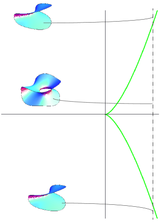
Let be a closed –manifold, and be a –dimensional surface. A map is said to have a cusp singularity at a point in , if around , is locally modeled in oriented charts by the map:
The critical point set is a smooth arc, , the critical value set is a cusp given by (see figure 1).
Following Lekili we state:
Definition 1.2.
A wrinkled fibration on a closed –manifold is a smooth map to a closed surface which is a broken fibration when restricted to , where is a finite set such that around each point in , has cusp singularities. We say that a fibration is purely wrinkled if it has no isolated Lefschetz-type singularities.
Wrinkled fibrations may be obtained from broken Lefschetz fibrations by performing wrinkling moves. These eliminate a Lefschetz type singularity and introduce a wrinkled fibration structure. Conversely, it is possible to modify a wrinkled fibration locally by smoothing out the cusp singularity by introducing a Lefschetz type singularity, so obtaining a broken fibration (see [8, 12]).
Next we will introduce the deformations of wrinkled fibrations that will appear in our Poisson strucures. As Lekili, by a deformation of wrinkled fibrations we mean a one-parameter family of maps which is a wrinkled fibration for all but finitely many values. One of Lekili’s major contributions in [8] was to show that any one-parameter family deformation of a purely wrinkled fibration is homotopic (relative endpoints) to one which realizes a sequence of births, merges, flips, their inverses, and isotopies staying within the class of purely wrinkled fibrations. Moreover, these moves do not change the diffeomorphism type of the –manifold on which they take place.
Let us briefly describe these moves, readers may consult both [8, 12] for the corresponding descriptions in terms of how the fibres change and how these moves can be described using handlebodies. The moves we are interested in are to be considered as maps , given by the following equations, each depending on a real parameter :
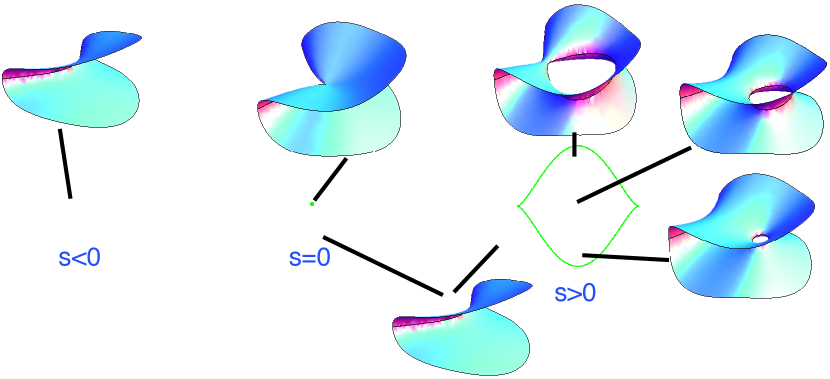
Move 1 (Birth, fig. 2)
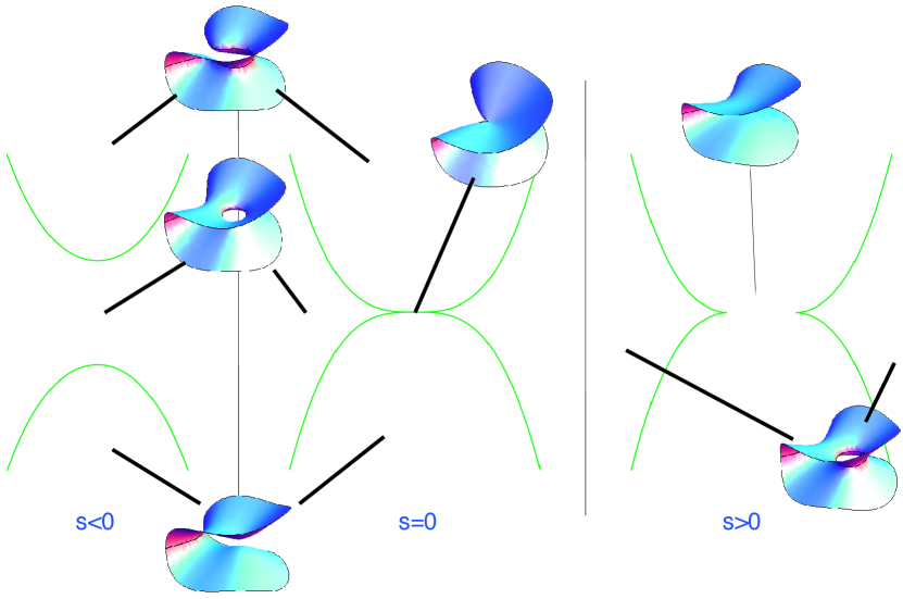
Move 2 (Merging, fig. 3)
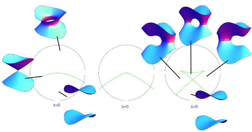
Move 3 (Flipping, fig. 4)
Move 4 (Wrinkling)
The proof of the existence of a Poisson structure presented in [6] also implies that there exists a Poisson structure associated to wrinkled fibrations, where the fibres are leaves of the symplectic foliation and both structures share the same singularities.
The constructions presented in this paper use a general procedure to construct Poisson structures with prescribed Casimir functions. These ideas, in a general context, can be traced back to Damianou’s thesis [3], to work of Damianou-Petalidou [4], and have also been attributed to Flaschka-Ratiu. However, the synthetic nature of the proof in [6], while complete, does not provide any information about the local forms of the Poisson bivector for wrinkled fibrations. The purpose of this note is to provide these details. In this paper, we continue to exploit the techniques of [6] in order present local formulæ for both the Poisson bivector and for the symplectic forms on the leaves of Poisson structures whose symplectic foliation and singularites are given by wrinkled fibrations and their deformations. Let us summarise the contributions of this paper in the following:
Theorem 1.3.
Let be a closed, orientable, smooth –manifold equipped with a wrinkled fibration, or for a fixed a fibration given by one of the birth, merging, flipping, or wrinkiling moves described above. Then there exists a complete Poisson structure whose symplectic leaves correspond to the fibres of the given fibration structure, and the singularities of both the fibration and the Poisson structures coincide. Moreover:
- (i)
- (ii)
- (iii)
- (iv)
- (v)
The existence of a Poisson structure with the stated properties follows from Theorem 2.4, originally shown in [6].
Given a Lie algebra , the integrability problem for was solved by Lie’s third theorem. It gives the existence of a Lie group such that . Crainic and Fernandes found obstructions for the integrability of Lie algebroids. Their main theorem in [2] establishes that any Poisson manifold whose symplectic leaves have trivial second homotopy groups is integrable.
Therefore we deduce:
Lemma 1.4.
Definitions and useful related results can be found in section 2. The computations of the bivectors and symplectic forms are carried out in section 3. We close with a brief appendix that describes the Mathematica code used to solve the differential equations that appear in the search for the local formulæ of the symplectic forms on the leaves.
Acknowledgements: We thank Gerardo Sosa for allowing us to use the figures in this paper, which originally appeared in [10], and Luis García-Naranjo for commenting on an earlier version. We thank the referees for suggesting how to simplify the computations, and for pointing out the relationships with integrability and linearization. PSS thanks CIMAT in Guanajuato for its warm hospitality in visits where this work was produced, and CONACyT-México for supporting various reasearch activities.
2. Definitions
2.1. Poisson manifolds
In this section we include basic facts about Poisson geometry that we will use throughout the paper. Interested readers are invited to consult [11, 5, 7].
Definition 2.1.
A Poisson bracket (or a Poisson structure) on a smooth manifold is a bilinear operation on the set of real valued smooth functions on that satisfies
-
(i)
is a Lie algebra.
-
(ii)
for any .
A manifold with such a Poisson bracket is called a Poisson manifold. Symplectic manifolds provide examples of Poisson manifolds. In the symplectic case the bracket of is defined by
Hamiltonian vector fields in symplect maniffolds are defined by .
Property (ii) in Definition 2.1 allows us to define Hamiltonian vector fields for Poisson manifolds. For we assign it the Hamiltonian vector field , defined via
It follows from (ii) that a Poisson bracket depends solely on the first derivatives of and . Hence we may think of the bracket as defining a bivector field defined by
| (2.1) |
A Poisson bivector can be described locally, for coordinates , by
Here .
Poisson brackets satisfy the Jacobi identity, which translates into a P.D.E. for the components of the Poisson bivector [7]. In this paper we will reformulate it for the class of bivectors we are interested in, so that it can be verified computationally (see Proposition LABEL:eqn:equivJacobi).
Given a bivector on , a point , and it is possible to to define:
When is Poisson, we have that .
We then define the rank of at to be equal to the rank of . This is also the rank of the matrix .
The distribution defined by on is called the characteristic distribution of . What is known as the Symplectic Stratification Theorem is the celebrated statement that this characteristic distribution of a Poisson tensor gives rise to a (possibly singular) foliation by symplectic leaves. This foliation is integrable in the sense of Stefan-Sussman [5].
Call the symplectic leaf of through the point . As a set is also the collection of points that may be joined via piecewise smooth integral curves of Hamiltonian vector fields. Write for the symplectic form on . Observe that is exactly the characteristic distribution of through . Therefore, given there exist that under go to and . Using this we can describe :
| (2.2) |
As the rank varies, so do the dimensions of the symplectic leaves of the foliation.
In the special case that the rank of the characteristic distribution of a bivector is less than or equal to two, the following were shown to hold in [6]:
Proposition 2.2.
-
(i)
If is a bivector field on whose characteristic distribution is integrable and has rank less than or equal to two at each point, then is Poisson.
-
(ii)
Let be a Poisson structure on whose rank at each point is less than or equal to two. Then is also a Poisson structure where is an arbitrary non-vanishing function.
In order to describe the bivectors locally we will use certain Casimir functions.
Definition 2.3.
Let be a Poisson manifold. A function is called a Casimir if for every .
Equivalently .
The next result was shown in [6]:.
Theorem 2.4.
Let be an orientable -manifold, an orientable manifold, and a smooth map. Let and be orientations of and respectively. The bracket on defined by
| (2.3) |
where is any non-vanishing function on is Poisson. Moreover, its symplectic leaves are
-
(i)
the 2-dimensional leaves where is a regular value of ,
-
(ii)
the 2-dimensional leaves where is a singular value of .
-
(iii)
the 0-dimensional leaves corresponding to each critical point.
Definition 2.5.
A Poisson manifold is said to be complete if every Hamiltonian vector field on is complete.
Notice that is complete if and only if every symplectic leaf is bounded in the sense that its closure is compact.
3. Local expressions for the Poisson structures.
3.1. Local forumlæ for the Poisson bivectors.
We will now construct explicit expressions for the Poisson structure and the corresponding symplectic forms in a neighbourhood of cusp singularities of wrinkled fibrations , as well as for all the possible moves described above. All of the expressions that we will give depend upon a choice of a non-vanishing function (see [6]).
Before proceeding we will describe the general strategy employed to find the local bivectors.
Step 1: Consider the coordinate functions that describe each fibration as Casimir functions for the Poisson structure that we want to find.
Step 2: Calculate the differentials of the Casimirs .
Step 3: We use formula 2.3 to compute the skew-symmetric matrix with entries:
This matrix will then annihilate , as this matrix is to be the endomorphism associated to a Poisson structure with and as Casimirs. The components of the bivector field will be given by:
Here is the canonical basis column vector, whose -th component is and all others are zero.
For the cusp singularity and the birth, merging, and flipping moves, is a Casimir, so we only have to compute
In fact, for these four cases if we denote by the components of the column vector we obtain
Step 4: According to Proposition 2.2 (ii), we write the Poisson bivector using the skew-symmetric matrix entries.
Near a wrinkling move the Poisson bivector will be obtained using formula 2.3. For the other cases the bivector admits a general expression given by:
| (3.1) |
for any non-vanishing smooth function .
The corresponding results for neighborhoods of Lefschetz singularities and broken singular circles were obtained in [6]. We proceed to describe the results this general strategy yields for cusp singularities and the moves described above.
Attentive readers might wonder why we are not using equation 2.3 directly. The computations needed to be carried out to take the volume form from the left hand side to the right hand side of the equation 2.3 are cumbersome and lengthy. The method we present below yields equivalent results, and may be easily verified.
3.1.1. Local expressions near a cusp singularity.
The local coordinate model around a cusp singularity is given by:
The differentials and are therefore:
The following matrix annihilates and and its entries satisfy the Jacobi identity :
Which means that the Poisson bivector in the local coordinates of a cusp singularity is described by:
| (3.2) |
3.1.2. Local expressions near a birth move.
The local coordinate model around a birth move is given by:
The differentials and are therefore:
From which we can obtain the following matrix:
Hence the Poisson bivector near a birth move has the form:
| (3.3) |
3.1.3. Local expressions near a merging move.
The local coordinate model around a merging move is given by:
The differentials and are therefore:
The associated matrix is then:
So the Poisson bivector in a neighbourhood of a merging move is described as:
| (3.4) |
3.1.4. Local expressions near a flipping move.
The local coordinate model around a flipping move is given by:
The differentials and are therefore:
The corresponding matrix is:
The Poisson bivector in a neighborhood of a flipping move can then be written in the following way:
| (3.5) |
3.1.5. Local expressions near a wrinkling move.
The local coordinate model around a wrinkling move is given by:
The differentials and are therefore:
The matrix we are interested in is given by:
The expression for the Poisson bivector in a neighbourhood of a wrinkling move is then:
| (3.6) |
3.1.6. Linearization
We follow chapters 3 and 4 of [5], where more details and examples may be found. Let be a finite-dimensional Lie algebra. Denote by the radical of , i.e., the maximal solvable ideal of . Then is a semi-simple Lie algebra. The Levi-Malcev theorem states that can be decomposed as a semi-direct product:
In analogy with this Levi-Malcev decomposition we have a Levi decomposition for Poisson structures. Let be a Poisson structure and denote by its linear part. By definition we obtain that generates a Lie algebra . We take the Levi-Malcev decomposition of , with the previous notation. Let be a basis for , such that span , and spans a complement of with respect to the adjoint action of on .
A Levi decomposition for at , with , provides local coordinates such that;
Any analytic Poisson structure , which vanishes at , admits a Levi decomposition in a neighborhood of .
Now we will focus on the expressions for the bivectors obtained in equations (3.2), (3.3), (3.4), (3.5), and (3.6). We fix . It can be seen that in the case of cusp singularities, the linear part of the corresponding Poisson structure (3.2) defines a Lie algebra through the commutation relations:
For the Birth, Merge and Flipping moves, corresponding to the bivectors (3.3), (3.4), and (3.5), respectively, their linear part in all these cases is generated by:
Notice that this Lie algebra contains a nonzero Abelian ideal, hence it is not semi-simple.
So in all these cases the linear part of the Poisson structure admits a decomposition of the form , where is a semi-direct product of Lie algebras:
Here acts on linearly by the matrix:
For the case of wrinkled fibrations, corresponding to (3.6), we see that all the commutation relations are trivial. Therefore the corresponding linear part of its Poisson structure spans an Abelian Lie algebra, which is not semi-simple.
Conn’s theorem asserts that, provided the linear part of an analytic Poisson structure that vanishes at , corresponds to a semi-simple Lie algebra, admits a local analytic linearizaton at . Hence, in the spirit of Conn’s theorem, the linearization of all these Poisson structures is not guaranteed. Moreover, the semi-direct product is degenerate (formally, analytically, and smoothly).
Finally, in the general case when is a non vanishing smooth function, we obtain other Poisson structures.
3.2. Equations for the symplectic forms on the leaves near singularities.
Proposition 3.2.
Let and let be the Poisson structure near a cusp singularity. Then the symplectic form induced by on the symplectic leaf through at the point is given by
| (3.7) |
here is the area form on induced by the euclidean metric on .
Proof.
If are tangent vectors to the leaves there exist co-vectors such that and , where is given by the rule:
Finding two tangent vectors to the symplectic leaves is equivalent to detecting vectors annihilated simultaneously by the differential of two Casimir functions for the corresponding Poisson structure. Note that the characteristic distribution has rank 2.
In this case we find that the vectors:
are tangent to at . Using the local expression of the Poisson structure for a cusp singularity given by equation (3.2), one can check that , for
Similarly, , for
A direct calculation now implies that the symplectic form is:
∎
Proposition 3.3.
Let and be the Poisson structure near a birth move. The symplectic form induced by on the symplectic leaf through at the point is given by
| (3.8) |
here is the area form on induced by the euclidean metric on .
Proof.
Making use of the corresponding Casimir functions for the Poisson structure associated to a birth move we obtain that the vectors
are tangent to at . Using the local expression (3.3) of the Poisson structure one can check that , for
Similarly, , for
The expression for the symplectic form follows from:
∎
Proposition 3.4.
Let and let be the Poisson structure near a merging move. The symplectic form induced by on the symplectic leaf through at the point is given by
| (3.9) |
here is the area form on induced by the euclidean metric on .
Proof.
We proceed similarly to the previous cases above. We find that the vectors
are tangent to at . Using the local expression (3.4) of the corresponding Poisson structure one can check that , for
Similarly, , for
As before the symplectic form is obtained by computing:
∎
Proposition 3.5.
Let and let be the Poisson structure near a flipping move. The symplectic form induced by on the symplectic leaf through at the point is given by
| (3.10) |
here is the area form on induced by the euclidean metric on .
Proof.
In this case, the following vectors:
are tangent to at . Using equation (3.5) we can check that , for
Similarly, , for
A straightforward calculation shows that:
∎
Proposition 3.6.
Let and let be the Poisson structure near a wrinkling move. The symplectic form induced by on the symplectic leaf through at the point is given by
| (3.11) |
here is the area form on induced by the euclidean metric on .
Proof.
Using the corresponding Poisson structure for a wrinkling move move given in equation (3.6) we obtain:
and makes an unitary vector. These vectors are tangent to at . Using the local expression of the Poisson structure in (3.6) we check that , for
Similarly, , for
The proposition is shown as in the previous cases by calculating the symplectic form explicitly using the above equations. ∎
References
- [1] D. Auroux, S. K. Donaldson, L. Katzarkov, Singular Lefschetz pencils, Geometry & Topology Vol. 9 (2005) 1043 –1114.
- [2] M. Crainic, R.L. Fernandes,Integrability of Lie brackets, Ann. of Math. (2) 157 (2003), no. 2, 575–620.
- [3] P. A. Damianou, Nonlinear Poisson Brackets. Ph.D. Dissertation, University of Arizona, 1989.
- [4] P. A. Damianou, F. Petalidou, Poisson Brackets with Prescribed Casimirs. Canadian J. Math. Vol. 64 (5), (2012), 991–1018.
- [5] J.-P. Dufour, N.T. Zung, Poisson structures and their normal forms, Progress in Mathematics, 242. Birkhäuser Verlag, Basel, 2005.
- [6] L. Gacía-Naranjo, P. Suárez-Serrato, R. Vera, Poisson structures on smooth –manifolds, Lett. Math. Phys., in press, arXiv:1406.7105v3.
- [7] C. Laurent-Gengoux, A. Pichereau, P. Vanhaecke, Poisson structures, Grundlehren der Mathematischen Wissenschaften, 347. Springer, Heidelberg, 2013.
- [8] Y. Lekili, Wrinkled fibrations on near-symplectic manifolds, Geometry & Topology 13 (2009), 277–318.
- [9] T. Perutz, Lagrangian matching invariants for fibred four-manifolds. I. Geom. Topol. 11 (2007), 759–828.
- [10] G. Sosa, Deformaciones de fibraciones corrugadas, Tesina de Maestría, Universidad Nacional Autónoma de México, 2013.
- [11] I. Vaisman, Lectures on the Geometry of Poisson Manifolds, Birkhäuser, Basel, 1994.
- [12] J. Williams, The h-principle for broken Lefschetz fibrations, Geometry & Topology 14 (2010), 1015–1061.