Integrability of Goldilocks quantum cellular automata

Abstract

Goldilocks quantum cellular automata (QCA) have been simulated on quantum hardware and produce emergent small-world correlation networks. In Goldilocks QCA, a single-qubit unitary is applied to each qubit in a one-dimensional chain subject to a balance constraint: a qubit is updated if its neighbors are in opposite basis states. Here, we prove that a subclass of Goldilocks QCA—including the one implemented experimentally—map onto free fermions and therefore can be classically simulated efficiently. We support this claim with two independent proofs, one involving a Jordan–Wigner transformation and one mapping the integrable six-vertex model to QCA. We compute local conserved quantities of these QCA and predict experimentally measurable expectation values. These calculations can be applied to test large digital quantum computers against known solutions. In contrast, typical Goldilocks QCA have equilibration properties and quasienergy-level statistics that suggest nonintegrability. Still, the latter QCA conserve one quantity useful for error mitigation. Our work provides a parametric quantum circuit with tunable integrability properties with which to test quantum hardware.

Introduction.—Classical cellular automata (CA) are dynamical models that evolve input bit strings (sequences of $1$s and $0$s) according to a simple local rule [1]. Typically, the update rule is the same everywhere along the bit string. At each time step, every bit is updated in accordance with its neighbors’ states. Despite their simplicity, CA engender rich dynamics, including order, randomness, fractals, and conservation laws. Also, CA can implement universal classical computation [2, 3]. Early CA work stressed conservation laws as ingredients for modeling physics [4, 5].

Classical CA generalize to quantum cellular automata (QCA), defined axiomatically as the unitary discrete dynamics that satisfy certain locality conditions [6, 7]. We focus on an important subset of QCA, digital QCA: constrained models implementable with quantum circuits of geometrically local gates. In digital QCA, each gate updates one or more qubits, in accordance with a surrounding neighborhood’s state. Prominent examples include the Goldilocks QCA, which generate small-world networks of bipartite mutual information [8, 9], and the Floquet PXP model [10], which exhibits quantum many-body scars [11, 12]. As unitary, closed-system models, digital QCA parallel reversible classical CA: QCA exhibit rich dynamical many-body features arising from the repeated application of simple local rules.

Quantum hardware recently simulated digital QCA [9]. The noisy experimental data were postselected to obey a conservation law. Consequently, complex networks of two-qubit correlators survived $>1000$ two-qubit gates. Do QCA conserve additional quantities? If enough quantities are conserved, can QCA dynamics be classically simulated efficiently? Identifying classically simulable quantum models restricts the scope of practical quantum advantage [13]. Also, classically simulable models provide many-qubit test cases for comparing emerging quantum computers with trusted classical counterparts.

Many physical systems conserve quantities such as energy, momentum, and particle number. Informally, a classical system is integrable if it conserves enough properties that it always evolves predictably. Two-body gravitational orbits and the harmonic oscillator exemplify classical integrabilty. In statistical physics, integrable systems include the two-dimensional Ising model [14] and the six-vertex model of ice [15, 16]. Some one-dimensional quantum models [17, 18, 19, 20] are integrable in that (i) the dynamics conserve extensively many local quantities and (ii) many-body interactions decompose into two-body interactions whose chronological ordering does not affect the physics. Yang-Baxter integrability codifies these two points, offering a working definition of quantum integrability [21]. Yang-Baxter integrability also interrelates classical, statistical, quantum-field, and quantum-lattice integrability [20, 22, 23, 24]. More recently, integrability has grown to include quantum circuits [25, 26, 27, 28, 29, 30, 31, 32, 33].

The simplest quantum-integrability setting involves noninteracting, or free, dynamics. Free fermions can be classically simulated efficiently [34, 35, 36]. Qubits can map onto fermions via the Jordan-Wigner (JW) transformation [17, 37, 38, 39]. However, it is nontrivial to identify whether a given unitary-gate sequence maps onto a noninteracting one .

We identify Goldilocks QCA that map onto free fermions, presenting two independent proofs. One relies on a JW transformation; and one, on a map from the integrable six-vertex model. Furthermore, we compute conserved quantities (charges) and use them to predict expectation values’ time-averaged thermodynamic limits. Efficient, finite-size classical simulations support our predictions. Unlike their free-fermionic counterparts, generic Goldilocks QCA appear nonintegrable according to three lines of evidence: each conserves only one local charge, local observables’ expectation values equilibrate to values predictable from that charge alone, and each QCA displays quasienergy-level statistics consistent with quantum chaos. Therefore, we present a parametric model that has tunable integrability properties and tunable conservation laws. More generally, our work elevates digital QCA as a practical tool for testing quantum hardware.

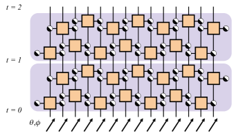
Figure 1: Goldilocks-QCA circuit. Each half-black-half-white circle represents one control of a generalized XOR constraint. The orange box represents the single-qubit unitary $\hat{V}$. The initial state is a tilted ferromagnet with a polar angle $\theta$ and azimuthal angle $\phi$.

Digital QCA.—We study a one-dimensional chain of qubits indexed by $j=0,1,\ldots,L-1$. $\{\ket{0},\ket{1}\}$ denotes the single-qubit computational basis; $\hat{\sigma}^{\gamma}_{j}$, the Pauli $\gamma\in\{x,y,z\}$ operator at qubit $j$; and $\hat{\mathbbm{1}}_{j}$, the identity. For notational convenience, we choose periodic boundary conditions, $j+L\equiv j$, and an even number $L$ of qubits. Our results do not depend on these choices.

$\ket{\Psi_{t}}$ denotes the system’s state at the discrete time $t$. $\ket{\Psi_{t}}$ is updated via spacetime-periodic applications of a local controlled-unitary gate. We focus on QCA of the following form. The gate is applied in a brickwork pattern: to all even-index qubits, then all odd-index ones (Fig. 1). During each time step, a single-qubit gate $\hat{V}\in{\rm SU}(2)$ may be applied to each qubit, depending on the states of that qubit’s neighbors. A unitary $\hat{U}$ on the Hilbert space $\mathcal{H}=(\mathbb{C}^{2})^{\otimes L}$ describes the dynamics: $\ket{\Psi_{t+1}}=\hat{U}(\hat{V})\ket{\Psi_{t}}$, wherein $\hat{U}(\hat{V})\coloneqq\hat{G}{(\hat{V},1)}\,\hat{G}{(\hat{V},0)}$. The global even-site/odd-site half-time-step gates are

$$\hat{G}{(\hat{V},q)}\coloneqq\prod_{k=0}^{L/2-1}\hat{u}_{2k+q}(\hat{V})\,,\quad q=0,1\,.$$ (1)

The neighborhood gates $\hat{u}_{j}(\hat{V})$ act on trios of qubits:

$$\hat{u}_{j}(\hat{V})\coloneqq\sum_{m,n=0}^{1}\ket{m}\!\bra{m}_{j-1}\otimes(\hat{V}_{j})^{f(m,n)}\otimes\ket{n}\!\bra{n}_{j+1}\,.$$ (2)

The left- and right-neighboring qubits form the controls. $f(m,n)\in\{0,1\}$ encodes the local update rule: if $f(m,n)=1$, while qubit $j$’s neighbors are in a state that overlaps with $\ket{m,n}_{j-1,j+1}$, then $\hat{V}$ updates qubit $j$’s state; otherwise, not. For example, the Floquet PXP model flips qubit $j$ if the neighbors are in the state $\ket{00}_{j-1,j+1}$. The corresponding $\hat{V}=\hat{\sigma}^{x}$, and $f_{\rm PXP}(m,n)=1-m\oplus n-mn$. The $\oplus$ denotes addition modulo $2$—the exclusive-or (XOR) classical logic gate. The Floquet Fredrickson-Andersen model [42, 43] flips a qubit if its neighbors are in any of the states $\ket{01}_{j-1,j+1}$, $\ket{10}_{j-1,j+1}$, or $\ket{11}_{j-1,j+1}$. This model’s $\hat{V}=\hat{\sigma}^{x}$, and $f_{\rm FA}(m,n)=m\oplus n+mn$. For Goldilocks QCA [8],

$$f_{\rm G}(m,n)=m\oplus n\,;$$ (3)

the neighbor configurations $\ket{01}_{j-1,j+1}$ and $\ket{10}_{j-1,j+1}$ enable nontrivial evolution. The name Goldilocks QCA comes from the rule’s updating qubit $j$ under more neighborhood conditions than the PXP model but fewer conditions than the Fredrickson-Andersen model—under a “just right” balance. When $\hat{V}=\hat{\sigma}^{x}$, Goldilocks QCA have been called the XOR-Fredrickson-Andersen model [44]. Our digital QCA generalize reversible CA and these previously studied models: $\hat{V}$ introduces additional degrees of freedom. Also, as we show, different $\hat{V}$ lead to integrable and seemingly nonintegrable dynamics. Henceforth, we denote by $\hat{U}(\hat{V})$ the Goldilocks-QCA time-step gate constructed with $\hat{V}$.

More-precise statement of results.—Goldilocks QCA generate free-fermionic dynamics if the single-site update unitary has the form

$$\hat{V}_{\rm free}(\alpha,\beta,\pm)\coloneqq\left(\begin{array}[]{cc}\cos\alpha&\mp e^{-i\beta}\sin\alpha\\ e^{i\beta}\sin\alpha&\pm\cos\alpha\end{array}\right)\,,\enspace\alpha,\beta\in\mathbb{R}.$$ (4)

The next section outlines a transparent proof based on a JW transformation. The following section overviews an independent proof, which maps the six-vertex model to the QCA. See the Supplemental Material (SM) for details [45].

This main result raises a question: are Goldilocks QCA with $\hat{U}(\hat{V}\neq\hat{V}_{\rm free})$ integrable? We demonstrate their consistency with nonintegrability. The most general single-site unitary is

$$\hat{V}^{\prime}(a,b)\coloneqq\frac{1}{\sqrt{|a|^{2}+|b|^{2}}}\left(\begin{array}[]{cc}a&b\\ -b^{*}&a^{*}\end{array}\right)\,,\quad a,b\in\mathbb{C}\,.$$ (5)

We draw the real and imaginary parts of $a$ and $b$ from independent standard normal distributions. The resultant $\hat{V}^{\prime}(a,b)$ likely lack finely tuned forms, such as (4). Hence we empirically quantify typical Goldilocks QCA’s local-charge, equilibration, and level-statistics properties. These properties suggest that typical Goldilocks QCA are nonintegrable, complementing the integrability we rigorously ascribe to $\hat{V}_{\rm free}$.

JW transformation.—We overview our first proof here (see Supplemental Note I for details), initially outlining the strategy. We decompose the neighborhood gate $\hat{u}_{j}$ into more-convenient elementary gates. Then, we define fermionic operators in terms of Pauli operators. We construct Hamiltonians that are bilinear (quadratic) in those fermion operators. These Hamiltonians generate unitaries that constitute the half-time-step operators $\hat{G}$. Due to the bilinearity, $\hat{G}$ represents free-fermionic evolution. For simplicity, we focus on single-site gates (4) with the restricted arguments $\hat{V}_{\rm free}(\alpha,0,-)$. The SM generalizes to arbitrary arguments.

Let us express the neighborhood gates conveniently. Denote by $[CZ]_{i,j}=\ket{0}\bra{0}_{i}\hat{\mathbbm{1}}_{j}+\ket{1}\bra{1}_{i}\hat{\sigma}^{z}_{j}$ the controlled-$Z$ gate between qubits $i$ and $j$. In terms of it, the neighborhood unitary (2) decomposes as $\hat{u}_{j}\bm{(}\hat{V}_{\rm free}(\alpha,0,-)\bm{)}=e^{-i(\alpha/2)\hat{\sigma}^{y}_{j}}[CZ]_{j-1,j}[CZ]_{j,j+1}e^{i(\alpha/2)\hat{\sigma}^{y}_{j}}$. Substituting this decomposition into Eq. (1), we express the half-time-step gates as $\hat{G}\bm{(}\hat{V}_{\rm free}(\alpha,0,-),\,q\bm{)}=e^{i\hat{H}_{1}(\alpha,q)}e^{-i\hat{H}_{2}}e^{-i\hat{H}_{1}(\alpha,q)}$. The Floquet Hamiltonians $\hat{H}_{1}$ and $\hat{H}_{2}$ depend on Pauli operators.

To JW-transform those Hamiltonians, we define fermionic annihilation operators :

$$\hat{a}_{j}\coloneqq\prod_{k=0}^{j-1}\hat{\sigma}^{y}_{k}\frac{(\hat{\sigma}^{z}_{j}+i\hat{\sigma}^{x}_{j})}{2}\,.$$ (6)

Under the JW transformation, the Floquet Hamiltonians are bilinear in the fermionic creation and annihilation operators:

$$\hat{H}_{1}(\alpha,q)\coloneqq-\frac{\alpha}{2}\sum_{j=0}^{L/2-1}\left(\hat{a}_{2j+q}\hat{a}_{2j+q}^{\dagger}-\hat{a}_{2j+q}^{\dagger}\hat{a}_{2j+q}\right)\,,\;\;\>{\rm and}$$ (7)

$$\hat{H}_{2}\coloneqq\frac{\pi}{4}\left[\pm\left(\hat{a}_{0}+\hat{a}_{0}^{\dagger}\right)\left(\hat{a}_{L-1}-\hat{a}_{L-1}^{\dagger}\right)\right.$$

$$\qquad\;+\left.\sum_{j=0}^{L-2}(-1)^{j+1}\left(\hat{a}_{j}^{\dagger}-\hat{a}_{j}\right)\left(\hat{a}_{j+1}+\hat{a}_{j+1}^{\dagger}\right)\right]\,.$$ (8)

The $\pm$ in (8) follows from a simplification (discussed in Supplemental Note I) familiar from the transverse-field Ising model’s JW transformation [37, 38]. The JW transformation (6) does not map the neighborhood gates (2) to Gaussian fermionic operators. Hence the QCA’s integrability is not obvious, a priori. We describe our second proof next.

Mapping from the six-vertex model.— The six-vertex model explains why H₂O-based ice has residual entropy at zero temperature [15]. Each molecule’s oxygen can participate in one of six configurations with its four neighbor-molecules’ hydrogens, obeying the ice condition [15, 16]; hence the name six-vertex. The model and its generalizations relate to other problems in statistical mechanics and quantum many-body physics [47, 48, 22]. Importantly, the model is exactly solvable [16, 49, 22].

In the original, classical model, each vertex type is associated with a Boltzmann weight. Two-dimensional such crystals are Yang-Baxter-integrable [16, 22] and, under certain conditions, noninteracting [49, 22]. However, this model (and closely related ones) can alternatively describe quantum dynamics [10, 31]. The vertex weights become complex-valued transition amplitudes. One of the crystal’s spatial dimensions becomes a discrete-time dimension. Furthermore, ice-conditioned vertices encode certain QCA neighborhood constraints. We impose the Goldilocks constraint and unitarity (see Supplemental Note II). The resulting instance of the six-vertex model both maps onto the Goldilocks update unitary $\hat{V}_{\rm free}$ [Eq. (4)] and is free-fermionic.

Our approach contrasts with recent work. The authors of [10, 50, 51] prove certain QCA’s Yang-Baxter integrability by constructing a transfer matrix. The transfer matrix generates extensively many mutually commuting charges, establishing integrabilty. We could similarly leverage the six-vertex model’s known transfer matrix [22] to calculate charges of our QCA. Alternatively, we could calculate charges from free-fermionic methods, as in [52, 53]. Instead, we next pursue an approach applicable to all $\hat{V}$, not only $\hat{V}_{\rm free}$: we numerically search for all charges with limited supports.

Conserved charges.—We identify charges by adapting the numerical algorithm of Ref. [54]. In principle, the algorithm returns all local charges (although not quasilocal ones). Finding less-local charges requires substantially more computational time. Let $\hat{A}^{(i)}\in\{\hat{\mathbbm{1}},\hat{\sigma}^{x},\hat{\sigma}^{y},\hat{\sigma}^{z}\}$ denote the $i^{\rm th}$ factor in a product of contiguous Pauli operators. We can sum such a product over all sites, $[\hat{A}^{(1)}\hat{A}^{(2)}\ldots\hat{A}^{(n)}]\coloneqq\sum_{j=0}^{L-1}\hat{A}^{(0)}_{j}\hat{A}^{(1)}_{j+1}\ldots\hat{A}^{(n)}_{j+n}$, or over all even-indexed sites: $[[\hat{A}^{(1)}\hat{A}^{(2)}\ldots\hat{A}^{(n)}]]\coloneqq\sum_{j=0}^{L/2-1}\hat{A}^{(0)}_{2j}\hat{A}^{(1)}_{2j+1}\ldots\hat{A}^{(n)}_{2j+n}$. Here $n$ denotes the size of a term’s support. We search for charges expressible in terms of such sums. A charge has a support size equal to the largest term’s support size.

We first focus on the single-site gates highlighted in the JW section, generalizing later: $\hat{U}{\bm{(}}\hat{V}_{\rm free}(\alpha,0,-)\bm{)}$, we find, conserves 13 linearly independent charges $\hat{Q}_{i=1,2,\ldots,13}$ of support size $\leq 5$. Having performed the search symbolically in Mathematica , we report eight charges needed later:

$$\hat{Q}_{1} =[\hat{\sigma}^{z}\hat{\sigma}^{z}],$$ (9a)

$$\hat{Q}_{2} =\tan\alpha\,[\hat{\sigma}^{x}\hat{\sigma}^{x}]+[\hat{\sigma}^{x}\hat{\sigma}^{z}]+[\hat{\sigma}^{z}\hat{\sigma}^{x}],$$ (9b)

$$\hat{Q}_{3} =[\hat{\sigma}^{x}\hat{\sigma}^{y}\hat{\sigma}^{z}]-[\hat{\sigma}^{z}\hat{\sigma}^{y}\hat{\sigma}^{x}],$$ (9c)

$$\hat{Q}_{4} =[\hat{\sigma}^{y}]+[\hat{\sigma}^{z}\hat{\sigma}^{y}\hat{\sigma}^{x}]+\tan\alpha\,[\hat{\sigma}^{x}\hat{\sigma}^{y}\hat{\sigma}^{z}],$$ (9d)

$$\hat{Q}_{5} =[\hat{\sigma}^{x}\hat{\sigma}^{x}]+[\hat{\sigma}^{z}\hat{\sigma}^{y}\hat{\sigma}^{y}\hat{\sigma}^{z}],$$ (9e)

$$\hat{Q}_{6} =\tan\alpha(\,[\hat{\sigma}^{x}\hat{\sigma}^{y}\hat{\sigma}^{y}\hat{\sigma}^{z}]-[\hat{\sigma}^{z}\hat{\sigma}^{y}\hat{\sigma}^{y}\hat{\sigma}^{z}])$$ (9f)

$$+[\hat{\sigma}^{x}\hat{\sigma}^{y}\hat{\sigma}^{y}\hat{\sigma}^{z}]+[\hat{\sigma}^{z}\hat{\sigma}^{y}\hat{\sigma}^{y}\hat{\sigma}^{x}],$$ (9g)

$$\hat{Q}_{7} =[\hat{\sigma}^{x}\hat{\sigma}^{y}\hat{\sigma}^{x}]-\tan\alpha([\hat{\sigma}^{x}\hat{\sigma}^{y}\hat{\sigma}^{z}]$$ (9h)

$$-[\hat{\sigma}^{x}\hat{\sigma}^{y}\hat{\sigma}^{y}\hat{\sigma}^{y}\hat{\sigma}^{z}])-[\hat{\sigma}^{z}\hat{\sigma}^{y}\hat{\sigma}^{y}\hat{\sigma}^{y}\hat{\sigma}^{x}],\;\>\text{and}$$ (9i)

$$\hat{Q}_{8} =[\hat{\sigma}^{x}\hat{\sigma}^{y}\hat{\sigma}^{y}\hat{\sigma}^{y}\hat{\sigma}^{z}]-[\hat{\sigma}^{z}\hat{\sigma}^{y}\hat{\sigma}^{y}\hat{\sigma}^{y}\hat{\sigma}^{x}]\,.$$ (9j)

Supplemental Note III specifies the remaining five charges. $\hat{Q}_{1}$ counts domain walls and is conserved by every update $\hat{V}$, even if $\hat{V}$ is chosen randomly at every site and circuit layer. Being diagonal relative to the computational basis, $\hat{Q}_{1}$ is useful for postselective error mitigation on quantum hardware [9].

The charges (9) do not all mutually commute. This observation is consistent with Ref. [53], since the dynamics map to a free-fermionic model that breaks one-site-translation symmetry. Exploring thermodynamic consequences of noncommuting charges is a recent endeavor [56, 57, 58, 59, 60]; now, Goldilocks QCA provide an additional example of non-Abelian integrability [61, 62, 63, 64].

Now, we generalize from $\hat{U}\bm{(}\hat{V}_{\rm free}(\alpha,0,-)\bm{)}$ in two ways. First, suppose that $\beta\neq 0$ in $\hat{V}_{\rm free}(\alpha,\beta,\pm)$ [Eq. (4)]. The charges follow from Eq. (9) and a local change of basis (see Supplemental Note I). Second, consider the plus-sign gates $\hat{V}_{\rm free}(\alpha,0,+)$. Using the algorithm of [54], we numerically found nine charges with support sizes $\leq 5$, for all $\alpha$ sampled. Only one charge—$\hat{Q}_{1}$—has a support size $\leq 3$. According to [51], at the point $\alpha=\pi/2$, $\hat{U}\bm{(}\hat{V}_{\rm free}(\pi/2,0,+)=\hat{\sigma}^{x}\bm{)}$ maps onto free evolution of domain walls (it conserves $\hat{Q}_{1}$) and conserves $\hat{Q}=[[\hat{I}\hat{\sigma}^{x}\hat{\sigma}^{x}\hat{I}]]+[[\hat{\sigma}^{z}\hat{\sigma}^{y}\hat{\sigma}^{y}\hat{\sigma}^{z}]]+[[\hat{\sigma}^{z}\hat{\sigma}^{z}\hat{\sigma}^{z}\hat{\sigma}^{z}]]$ . In addition to proving this QCA’s free-fermionic nature, we numerically demonstrate that each of the three terms in $\hat{Q}$ is conserved individually. Furthermore, we find 24 charges with support sizes $\leq 5$ at $\alpha=\pi/2$.

Finally, we illustrate generic Goldilocks QCA, whose single-site update unitaries $\hat{V}^{\prime}(a,b)$ are selected as specified around Eq. (5). Using the algorithm of Ref. [54], we find no charges (except $\hat{Q}_{1}$) with support size $\leq 5$ for the representative example $\hat{U}\bm{(}\hat{V}^{\prime}(0.3+0.7i,-1.0-0.5i)\bm{)}$. This outcome, as well as evidence presented next, suggests that generic Goldilocks QCA are nonintegrable. Nevertheless, fine-tuned $\hat{V}^{\prime}$ choices might engender (interacting) integrable dynamics that one might find using methods like those in Ref. [51].

Predicting dynamics.—We now contrast integrable and generic QCA dynamics. We initialize the system in the translationally invariant, tilted-ferromagnet product state $\ket{\Psi_{0}(\theta,\phi)}\coloneqq\ket{\theta,\phi}^{\otimes L}$, where $\ket{\theta,\phi}\coloneqq\cos(\theta/2)\ket{0}+e^{i\phi}\sin(\theta/2)\ket{1}$. We calculate the evolutions of local expectation values

$$\mathcal{F}(t;\gamma,k)\coloneqq\braket{\Psi_{t}}{(\hat{\sigma}^{\gamma})^{\otimes k}}{\Psi_{t}}\,.$$ (10)

As a first consequence of free-fermion integrability, $\mathcal{F}(t;\gamma,k)$ can be classically simulated efficiently, via the Gaussian formalism [35, 36], for diverse initial states. These are the states mapped, via the JW transformation, onto Gaussian states. Gaussian states are fully specified by their covariance matrices, and expectation values in Gaussian states follow from Wick’s theorem [35]. The set of Gaussian states includes the $y$-ferromagnet state, $\ket{\Psi_{0}(\pi/2,\pi/2)}=[(\ket{0}+i\ket{1})/\sqrt{2}]^{\otimes L}$.

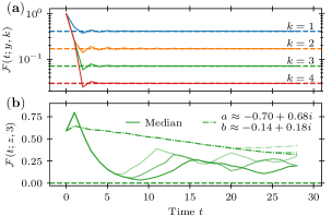
Figure 2: Expectation-value dynamics. (a) Dynamics generated by integrable Goldilocks QCA $\hat{U}[\hat{V}_{\rm free}(\pi/4,0,-)]$, for a system size $L=256$. The initial (Gaussian) state is the $y$-ferromagnet. (b) Median expectation value from 100 realizations of generic Goldilocks QCA $\hat{U}[\hat{V}^{\prime}(a,b)]$ (solid curves) and one outlying realization [$96^{\rm th}$ percentile of $\mathcal{F}(9;z,3)$, dot-dashed curves]. Darker curves signal larger system sizes ($L=18,22,26$). The initial state is the tilted ferromagnet $\ket{\Psi_{0}(0.56,3.7)}$. In both panels, horizontal dashed curves mark the thermodynamic limits predicted by the appropriate GGE.

We have efficiently calculated the expectation values (10) numerically. See Supplemental Note IV for details. Figure 2(a) illustrates our results. It shows expectation values $\mathcal{F}(t;y,k)$ of the experimentally realized Goldilocks QCA, whose $\hat{V}=\hat{V}_{\rm free}(\pi/4,0,-)$ [9].

In contrast, we cannot apply the Gaussian formalism to generic QCA. The numerical computations involve brute-force representations of the evolution operators in the computational basis. Only small sizes and times are achievable. Figure 2(b) illustrates the median (and one example outlier) of expectation values $\mathcal{F}(t;z,3)$ calculated from 100 $\hat{V}^{\prime}(a,b)$ realizations. (In each realization, the same $\hat{V}^{\prime}(a,b)$ acted at each site and time step.)

A second consequence of integrability pertains to the expectation values’ time-averaged, large-system limits. In the thermodynamic limit, expectation values are expected to be consistent with generalized Gibbs ensembles (GGEs) [66, 67, 68]

$$\hat{\rho}\coloneqq\frac{1}{Z}\exp\left(-\sum_{i}\hat{Q}_{i}\mu_{i}\right)\,.$$ (11)

The sum runs over the local charges. The normalization factor $Z\coloneqq\mathrm{Tr}\bm{(}\exp(-\sum_{i}\hat{Q}_{i}\mu_{i})\bm{)}$. The $\mu_{i}$ are generalized chemical potentials (or Lagrange multipliers) fixed by the initial conditions: $\bra{\Psi_{0}}\hat{Q}_{i}\ket{\Psi_{0}}=\mathrm{Tr}(\hat{\rho}\hat{Q}_{i})$. If one does not know all the charges, one can truncate the GGE  [52, 69]—construct the approximate ensemble $\hat{\rho}^{[n]}$ that includes the $m$ charges of support size $\leq n$ . Truncated-GGE predictions approximate GGE predictions of expectation values with support sizes $<n$ [52]. For systems whose charges commute, Eq. (11) predicts time-averaged expectation values of a large system prepared in a microcanonical subspace—with well-defined values of the included charges [71]. If the charges fail to commute, Eq. (11) predicts analogously for a system in an approximate microcanonical subspace—with fairly well-defined values of the included charges (since noncommuting charges cannot necessarily have well-defined values simultaneously) [59, 72, 73]. Our initial condition, being a product state, satisfies this requirement [72].

We computed truncated-GGE predictions $\mathrm{Tr}(\hat{\rho}^{[n]}[\hat{\sigma}^{\gamma}]^{\otimes k})$ for our free-fermion and generic systems. Figure 2(a–b) shows these results and comparisons with the exact time-evolved expectation values. The free-fermion case involves the 13 local charges described around Eqs. (9). The chemical potentials $\mu_{i}=0$ (up to our method’s numerical accuracy) for $i>m=8$. The time-evolved expectation values rapidly equilibrate to the truncated-GGE predictions. As $k$ increases, the equilibrium value approaches zero. Supplemental Note V explains this behavior qualitatively, although it is unimportant for our purposes.

Generic Goldilocks QCA conserve only $\hat{Q}_{1}$: $n=2$, and $m=1$. The tilted ferromagnet with polar angle $\theta$ implies $\mu_{1}={\rm arctanh}(\cos^{2}\theta)$ and $\mathrm{Tr}(\hat{\rho}^{[2]}[\hat{\sigma}^{z}]^{\otimes k})=[\cos^{k}\theta+(-\cos\theta)^{k}]/2$, by direct calculation (Supplemental Note V). We calculate the median expectation value over 100 $V^{\prime}(a,b)$ realizations. It behaves as $\mathcal{F}(t,z,3)\to 0$, approaching the truncated-GGE prediction, as $L$ increases. Outliers converge slowly in time and $L$. Possible reasons include (i) proximity to integrable points and (ii) conserved charges undetected by our method.

Level statistics.—(Quasi)energy-level statistics can evidence integrability [54, 74, 50]. This evidence is reliable, though, only if computed from energy levels in the same symmetry sector. As detailed in Supplemental Note VI, we analyze spectral statistics in a sector shared by two charges: first, $\hat{Q}_{1}$ has eigenvalues $q_{1}\in{-L,-L+4,\ldots,L}$. Second, every $\hat{V}^{\prime}$ conserves the two-site-shift operator $\hat{\Pi}^{2}$. Its eigenvalues $e^{4\pi iK/L}$ depend on $K\in\{0,1,\ldots,L/2\}$. In an eigenspace shared by $\hat{\Pi}^{2}$ and $\hat{Q}_{1}$, we compute eigenvalues $e^{i\phi_{\ell}}$ of the time-step unitary $\hat{U}$, following [50]. We sort the quasienergies $\phi_{\ell}\in[0,2\pi)$ in ascending order. From the spacings $s_{\ell}\coloneqq\phi_{\ell+1}-\phi_{\ell}$, we form ratios [75] $r_{\ell}\coloneqq\min\{s_{\ell},s_{\ell-1}\}/\max\{s_{\ell},s_{\ell-1}\}$. $P(r)$ denotes the distribution, across the quasienergy spectrum, over these ratios. $P(r)$ is more convenient than the distribution over the spacings themselves, which require spectral-unfolding analyses [75, 76, 74]. Poisson statistics $P_{\rm P}(r)=2/(1+r)^{2}$ can signal integrability [77], whereas Wigner-Dyson statistics $P_{\rm WD}(r)=(27/4)(r+r^{2})/(1+r+r^{2})^{5/2}$ can signal nonintegrability [78].

Figure 3 shows the level statistics of typical single-site update operators $\hat{V}^{\prime}(a,b)$. Different realizations evidence Wigner-Dyson-like, Poisson-like, and intermediate statistics. The median distribution is closest to Wigner-Dyson. Furthermore, the fraction displaying Wigner-Dyson-like statistics grows with $L$. Therefore, most Goldilocks QCA appear nonintegrable.

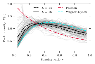
Figure 3: Quasienergy-level statistics. Distribution $P(r)$ over level-spacing ratios. The solid black curve shows the median distribution, calculated from 100 realizations of $\hat{V}^{\prime}(a,b)$ at $L=16$, from the $(K{=}1,\,q_{1}{=}0)$ sector’s 3200 levels. The faint curves show individual realizations. The black dashed line shows the median distribution for the same 100 $\hat{V}^{\prime}$ realizations but a smaller system ($L=14$) and the $(K{=}1,\,q_{1}{=}2)$ sector’s 858 levels.The Wigner-Dyson (dashed, cyan) and Poisson (dot-dashed, red) distributions serve as references.

Outlook.—We have proven that certain Goldilocks QCA exhibit free-fermionic integrability. This claim rests on two independent proofs, one involving a Jordan–Wigner transformation; and one, a mapping from the six-vertex model. We demonstrated implications of integrability: efficient classical simulability, many (noncommuting) local charges, and rapid equilibration to truncated-GGE predictions. Generic Goldilocks QCA are predominately consistent with nonintegrability, as evidenced by thermalization to single-charge-GGE predictions and Wigner-Dyson-like level statistics.

Some QCA exhibit anomalous behaviors that invite future research: intermediate level statistics and thermalization that is less complete, as a function of $L$, than one might expect. Noncommuting charges can enable such behaviors, as might near-integrability. Do generic QCA lie close to integrable parameter points, conserve hidden noncommuting charges, or approximately conserve noncommuting charges? Noncommuting-charge studies have focused on exact conservation [56]. Extensions to approximate conservation could uncover further quantum thermodynamics, and Goldilocks QCA might provide a toy model.

Our integrability proofs raise more questions. Our six-vertex map works for many QCA (see Supplemental Note II) but, applied to Goldilocks QCA, reveals noninteracting integrability. Could other six-vertex QCA exhibit interacting or nonunitary integrability [79, 80]? Can all the QCA that map onto free fermions be classified? One can straightforwardly generalize our discovered free-fermion dynamics by maintaining the Goldilocks constraint, while targeting $\geq 2$ qubits with $\hat{V}$ (Supplemental Note VII). More generally, could free fermions in disguise, like those in Ref. [81], appear in QCA? The very recent paper [32] suggests so. Answers to these questions may further identify candidate settings for practical quantum advantages and provide reliable data for many-qubit benchmarking experiments.

Acknowledgements.—We acknowledge useful conversations with Ehud Altman, Mina Fasihi, Matthew Jones, Norman Margolus, and Andrew Potter. This work was performed in part with support by the U.S. National Science Foundation under grants PHY-2210566 and OMA-2120757, and Slovenian Research and Innovation Agency (ARIS) under grants P1-0402, N1-0334, N1-0219 (TP).

Supplemental Material for “Integrability of Goldilocks quantum cellular automata”

Appendix I Details about the Jordan-Wigner mapping of certain Goldilocks quantum cellular automata to free fermions

In this section, we detail the JW mapping of certain Goldilocks QCA [those described by Eq. (SII.32)] to noninteracting Floquet dynamics. Specifically, we show that bilinear fermionic Hamiltonians generate the global time-step unitaries $\hat{U}\bm{(}\hat{V}_{\rm free}(\alpha,\beta,\pm)\bm{)}$. We first prove the result for restricted arguments $\hat{V}_{\rm free}(\alpha,0,-)$, then generalize afterward. As outlined in the main text, we first decompose the neighborhood gate $\hat{u}_{j}$ [Eq. (2)] into simpler one- and two-qubit gates. We then apply this decomposition to the half-time-step gates $\hat{G}$ [Eq. (1)]. Performing a JW transformation reveals that each $\hat{G}$ is bilinear in the JW fermions.

For convenience, we first analyze the neighborhood gate $\hat{u}_{j}$ [Eq. (2)] with the restricted argument $\hat{V}_{\rm free}(\alpha,0,-)$. This gate decomposes into one- and two-qubit gates, one can verify by direct computation:

$$\hat{u}_{j}\bm{(}\hat{V}_{\rm free}(\alpha,0,-)\bm{)}=e^{-i(\alpha/2)\,\hat{\sigma}^{y}_{j}}\,[CZ]_{j-1,j}\,[CZ]_{j,j+1}\,e^{i(\alpha/2)\hat{\sigma}^{y}_{j}}\,.$$ (SI.1)

In terms of these neighborhood gates, the even ($q=0$) and odd ($q=1$) half-time-step operators are

$$\hat{G}\bm{(}\hat{V}_{\rm free}(\alpha,0,-),q\bm{)} =\prod_{j=0}^{L/2-1}\hat{u}_{j}\bm{(}\hat{V}_{\rm free}(\alpha,0,-)\bm{)}$$

$$=\left(\prod_{j=0}^{L/2-1}e^{-i(\alpha/2)\hat{\sigma}_{2j+q}^{y}}\right)\left(\prod_{j=0}^{L/2-1}[CZ]_{j-1,j}[CZ]_{j,j+1}\right)\left(\prod_{j=0}^{L/2-1}e^{i(\alpha/2)\hat{\sigma}_{2j+q}^{y}}\right).$$ (SI.2)

The controlled-$Z$ gate decomposes in terms of Pauli operators as

$$[CZ]_{j,j+1}=e^{-i\pi/4}\,\exp\left(-i\frac{\pi}{4}\,\hat{\sigma}^{z}_{j}\,\hat{\sigma}^{z}_{j+1}\right)\,\exp\left(+i\,\frac{\pi}{4}\left[\hat{\sigma}^{z}_{j}+\hat{\sigma}^{z}_{j+1}\right]\right).$$ (SI.3)

Therefore, the second factor in Eq. (SI.2) is

$$\prod_{j=0}^{L/2-1}[CZ]_{j-1,j}[CZ]_{j,j+1} =\prod_{j=0}^{L-1}[CZ]_{j,j+1}$$ (SI.4)

$$=\prod_{j=0}^{L-1}\exp\left(-i\frac{\pi}{4}\hat{\sigma}^{z}_{j}\hat{\sigma}^{z}_{j+1}\right)\exp\left(i\frac{\pi}{4}\left[\hat{\sigma}^{z}_{j}+\hat{\sigma}^{z}_{j+1}\right]\right)$$

$$=\exp\left(-i\frac{\pi}{4}\sum_{j=0}^{L-1}\hat{\sigma}^{z}_{j}\hat{\sigma}^{z}_{j+1}\right)\exp\left(i\frac{\pi}{2}\sum_{j=0}^{L-1}\hat{\sigma}^{z}_{j}\right)$$

$$=i^{L}\exp\left(-i\frac{\pi}{4}\sum_{j=0}^{L-1}\hat{\sigma}^{z}_{j}\hat{\sigma}^{z}_{j+1}\right)\prod_{k=0}^{L-1}\hat{\sigma}^{z}_{k}\,.$$ (SI.5)

The final equality follows from $e^{i(\pi/2)\hat{\sigma}^{z}}=i\hat{\sigma}^{z}$. Similarly, $\hat{\sigma}^{z}_{k}\hat{\sigma}^{z}_{k+1}=-i\exp\left(i\frac{\pi}{2}\hat{\sigma}^{z}_{k}\hat{\sigma}^{z}_{k+1}\right)$, so the final factor in (SI.5) is

$$\prod_{k=0}^{L-1}\hat{\sigma}^{z}_{k}=\prod_{k=0}^{L/2-1}\hat{\sigma}^{z}_{2k}\hat{\sigma}^{z}_{2k+1}=(-i)^{L/2}\exp\left(i\frac{\pi}{2}\sum_{j=0}^{L/2-1}\hat{\sigma}^{z}_{2k}\hat{\sigma}^{z}_{2k+1}\right).$$ (SI.6)

We substitute from Eq. (SI.6) into Eq. (SI.5), then substitute the result into Eq. (SI.2). Neglecting the global phase,

$$\hat{G}\bm{(}\hat{V}_{\rm free}(\alpha,0,-),q\bm{)}=\exp\left(\frac{-i\alpha}{2}\sum_{j=0}^{L/2-1}\hat{\sigma}^{y}_{2j+q}\right)\exp\left(\frac{-i\pi}{4}\left\{\hat{\sigma}^{z}_{L-1}\hat{\sigma}^{z}_{0}+\sum_{j=0}^{L-2}[-1]^{j+1}\hat{\sigma}^{z}_{j}\hat{\sigma}^{z}_{j+1}\right\}\right)\exp\left(\frac{i\alpha}{2}\sum_{k=0}^{L/2-1}\hat{\sigma}^{y}_{2j+q}\right).$$ (SI.7)

We define the two Hamiltonians

$$\hat{H}_{1}(\alpha,\,q) \coloneqq-\frac{\alpha}{2}\sum_{j=0}^{L/2-1}\hat{\sigma}^{y}_{2j+q}\qquad\text{and}\qquad\hat{H}_{2}\coloneqq\frac{\pi}{4}\left[\hat{\sigma}^{z}_{L-1}\hat{\sigma}^{z}_{0}+\sum_{j=0}^{L-2}(-1)^{j+1}\hat{\sigma}^{z}_{j}\hat{\sigma}^{z}_{j+1}\right]\,,$$ (SI.8)

so that $\hat{G}\bm{(}\hat{V}_{\rm free}(\alpha,0,-),\,q\bm{)}=\exp\bm{(}+iH_{1}(\alpha,q)\bm{)}\exp(-iH_{2})\exp\bm{(}-iH_{1}(\alpha,q)\bm{)}$.

As in the main text, we introduce the fermionic annihilation operators $\hat{a}_{j}$ via the JW transformation:

$$\hat{a}_{j}=\prod_{k=0}^{j-1}\hat{\sigma}^{y}_{k}\,\frac{(\hat{\sigma}^{z}_{j}+i\hat{\sigma}^{x}_{j})}{2}\,.$$ (SI.9)

From the creation and annihilation operators, we can build bilinear fermionic operators such as $\hat{\sigma}^{y}_{j}=\hat{a}_{j}\hat{a}_{j}^{\dagger}-\hat{a}_{j}^{\dagger}\hat{a}_{j}$ and $\hat{\sigma}^{z}_{j}\hat{\sigma}^{z}_{j+1}=(\hat{a}_{j}^{\dagger}-\hat{a}_{j})(\hat{a}_{j+1}+\hat{a}_{j+1}^{\dagger})$. From the first such operator, in turn, we construct the fermion-number-parity operator:

$$\hat{\mathcal{P}}=\prod_{j=0}^{L-1}\hat{\sigma}^{y}_{j}=\prod_{j=0}^{L-1}\left(\hat{a}_{j}\hat{a}_{j}^{\dagger}-\hat{a}_{j}^{\dagger}\hat{a}_{j}\right)\,.$$ (SI.10)

The number-parity operator features in one of the Hamiltonians we defined: applying the JW transformation (SI.9) to Eqs. (SI.8) yields

$$\hat{H}_{1}(\alpha,q) =-\frac{\alpha}{2}\sum_{j=0}^{L/2-1}\left(\hat{a}_{2j+q}\hat{a}_{2j+q}^{\dagger}-\hat{a}_{2j+q}^{\dagger}\hat{a}_{2j+q}\right)\quad\text{and}$$ (SI.11)

$$\hat{H}_{2} =\frac{\pi}{4}\left[\left(\hat{a}_{0}+\hat{a}_{0}^{\dagger}\right)\left(\hat{a}_{L-1}-\hat{a}_{L-1}^{\dagger}\right)\hat{\mathcal{P}}+\sum_{j=0}^{L-2}(-1)^{j+1}\left(\hat{a}_{j}^{\dagger}-\hat{a}_{j}\right)\left(\hat{a}_{j+1}+\hat{a}_{j+1}^{\dagger}\right)\right].$$ (SI.12)

$\hat{H}_{1}$ is overtly quadratic in the fermion operators, even if different $\alpha$ values are assigned to different sites. In contrast, $\hat{H}_{2}$ is not overtly quadratic.

Nevertheless, we can prove that $\hat{G}\bm{(}\hat{V}_{\rm free}(\alpha,0,-),\,q\bm{)}$ is free-fermionic by invoking the number-parity operator. The operator commutes with both Hamiltonians: $[\hat{H}_{2},\hat{\mathcal{P}}]=[\hat{H}_{1}(\alpha,q),\hat{\mathcal{P}}]=0$. Each $\hat{H}$ can be therefore represented, relative to the $\hat{\mathcal{P}}$ eigenbasis, by a block-diagonal matrix. Each matrix consists of two blocks, as $\hat{\mathcal{P}}$ has two eigenvalues, $\pm 1$. Denote the $+1$ eigenstates by $\ket{\varphi_{+}^{(j)}}$ and the $-1$ eigenstates by $\ket{\varphi_{-}^{(k)}}$, for indices $j$ and $k$. In terms of these eigenstates, an arbitrary pure state decomposes as $\ket{\Psi}=\sum_{j}c_{+}^{(j)}\ket{\varphi_{+}^{(j)}}+\sum_{j}c_{-}^{(k)}\ket{\varphi_{-}^{(k)}}$, for normalized coefficients $c_{+}^{(j)},c_{-}^{(k)}\in\mathbb{C}$. Consider operating with the $\hat{H}_{2}$ matrix on $\ket{\Psi}$. Whenever the matrix acts on a $\ket{\varphi_{+}^{(j)}}$ term, the $\hat{\mathcal{P}}$ in Eq. (SI.12) acts as $+1$; and, when the matrix acts on a $\ket{\varphi_{-}^{(k)}}$ term, the $\hat{\mathcal{P}}$ as a $-1$. Hence, by Eq. (SI.12), $\hat{H}_{2}$ always acts as a quadratic operator. Both half-time-step operators $\hat{G}$ are therefore quadratic. Consequently the global evolution operator $\hat{U}(\hat{V}_{\rm free})=\hat{G}(\hat{V}_{\rm free},\,1)\hat{G}(\hat{V}_{\rm free},\,0)$ can be rewritten as

$$\hat{U}\bm{(}\hat{V}_{\rm free}(\alpha,0,-)\bm{)}=e^{i\hat{H}_{1}(\alpha,\,1)}\,e^{-i\hat{H}_{2}}\,e^{-i\hat{H}_{1}(\alpha,\,1)}\,e^{i\hat{H}_{1}(\alpha,\,0)}\,e^{-i\hat{H}_{2}}\,e^{-i\hat{H}_{1}(\alpha,\,0)}\,.$$ (SI.13)

Hence the Goldilocks-QCA time-step operator effects free-fermion dynamics.

One could further simplify Eq. (SI.13) to compute the Floquet Hamiltonian $\hat{K}$ that satisfies $\hat{U}=e^{-i\hat{K}}$. One would Fourier-transform Eq. (SI.13), then apply the Baker–Campbell–Hausdorff formula. Finally, one would invoke the fact that any two quadratic operators’ commutator is a quadratic operator. See Ref. [30] for a similar computation. However, we do not use the form of $\hat{K}$, so we omit this computation.

We now relax the restrictions imposed on the arguments of $\hat{V}_{\rm free}$ [Eq. (4)]: the $\beta$ and then the minus sign. The already-analyzed operator $\hat{V}(\alpha,0,-)$ transforms into the less restricted operator $\hat{V}_{\rm free}(\alpha,\beta,-)$ under the local basis change $e^{-i(\beta/2)\hat{\sigma}^{z}}$: $\hat{V}_{\rm free}(\alpha,\beta,-)=e^{-i(\beta/2)\hat{\sigma}^{z}}\hat{V}(\alpha,0,-)e^{i(\beta/2)\hat{\sigma}^{z}}$. The basis change preserves the QCA’s free-fermionic structure, merely rotating the Pauli operators in the JW transformation (6):

$$\hat{\sigma}^{x}\to\cos\beta\,\hat{\sigma}^{x}+\sin\beta\,\hat{\sigma}^{y}\,,\quad\text{and}\quad\hat{\sigma}^{y}\to\sin\,\beta\hat{\sigma}^{x}+\cos\,\beta\hat{\sigma}^{y}\,.$$ (SI.14)

One must transform also the charges (9) under (SI.14), to calculate the $\beta\neq 0$ charges.

Finally, we prove the free-fermion nature of $\hat{V}_{\rm free}(\alpha,\beta,+)$. Direct calculation reveals $u_{j}\bm{(}\hat{V}_{\rm free}(\alpha,\beta,+)\bm{)}=[CZ]_{j-1,j}[CZ]_{j,j+1}u_{j}\bm{(}\hat{V}_{\rm free}(-\alpha,\beta,-)\bm{)}$. Therefore, one can simulate the $\hat{V}_{\rm free}(\alpha,\beta,+)$, using $\hat{V}_{\rm free}(\alpha,\beta,-)$: one negates $\alpha$ and includes an extra layer of controlled-$Z$ gates:

$$\hat{G}\bm{(}\hat{V}_{\rm free}(\alpha,\beta,+),\,q\bm{)}=\prod_{j=0}^{L-1}[CZ]_{j,j+1}\hat{G}\bm{(}\hat{V}_{\rm free}(-\alpha,\beta,-)\bm{)}.$$ (SI.15)

If $\beta=0$, the global evolution operator is

$$\hat{U}\bm{(}\hat{V}_{\rm free}(\alpha,0,+)\bm{)}=e^{-i\hat{H}_{2}}\,e^{i\hat{H}_{1}(-\alpha,\,1)}\,e^{-i\hat{H}_{2}}\,e^{-i\hat{H}_{1}(-\alpha,\,1)}\,e^{-i\hat{H}_{2}}\,e^{i\hat{H}_{1}(-\alpha,\,0)}\,e^{-i\hat{H}_{2}}\,e^{-i\hat{H}_{1}(-\alpha,\,0)}\,.$$ (SI.16)

If $\beta\neq 0$, we can apply the same construction, together with the local basis rotation (SI.14).

Appendix II Mapping from the six-vertex model

In this section, we detail the mapping from the six-vertex model to certain Goldilocks QCA. We start by recalling elementary facts about the model. Then, we show that the six-vertex model maps onto a set of QCA neighborhood gates. This set of gates overlaps partially with the set of QCA neighborhood gates $\hat{u}_{j}(\hat{V})$ focused on in this paper [Eq. (2)]. Finally, we identify the Goldilocks QCA mapped to by points in the six-vertex model’s parameter space. At these points, we show, the six-vertex model is free-fermionic.

II.1 Six-vertex model

The six-vertex model [22] is defined on a lattice whose degrees of freedom are the edges. Each edge is empty or occupied—or, equivalently, carries an orientation: upwards for empty edges and downwards for occupied edges. The net flux flowing into each vertex must vanish. According to this ice condition, the allowed vertices are

(SII.17)

As originally formulated, the six-vertex model is a classical statistical-mechanics model in two spatial dimensions. Each vertex is assigned a positive Boltzmann weight—$a_{1}$, $a_{2}$, $b_{1}$, $b_{2}$, $c_{1}$, or $c_{2}$—as indicated above. A lattice configuration has a Boltzmann weight equal to the product of its vertices’ weights. The model’s partition function is the sum over the configurations’ lattice weights. The six-vertex model’s parameter space has free-fermionic points specified by the condition $a_{1}a_{2}+b_{1}b_{2}=c_{1}c_{2}$ [49, 22].

This vertex model, whose degrees of freedom are the edges, is equivalent to a model whose degrees of freedom are spins [48, 47, 22, 24]. Let a classical spin live on each face of each vertex, such that the vertex becomes the center of a plaquette. We represent an upward-pointing spin with a 0 and a downward-pointing spin with a 1. The vertex model is equivalent to this spin model under the following rule: empty (filled) lattice edges separate neighboring spins that are aligned (antialigned). Two plaquette configurations are consistent with each of the six vertex configurations . These ice-conditioned plaquettes, and the corresponding weights, are

(SII.18)

Instead of representing a classical spin system in two spatial dimensions, the six-vertex model can represent a one-dimensional quantum system evolving in discrete time [10]. The classical lattice’s $y$-axis can be reinterpreted as the quantum system’s time axis, which runs from bottom to top. Consecutive lattice rows represent the quantum system’s state at consecutive time steps. Similarly to in the classical spin model, a qubit lives on each face of each vertex. Each qubit’s Hilbert space has a computational basis $\{\ket{0},\ket{1}\}$. If a qubit is in $\ket{0}$ ($\ket{1}$), we say that the spin is pointing upward (downward). Within a row, the southward spins specify the system’s state at some time, and the northward spins specify the system’s state at the next time step. Enforcing the ice condition constrains the qubits’ evolution. Specifying the evolution, we specify, for each qubit, the complex amplitudes for the transitions $(0\to 0)$, $(0\to 1)$, $(1\to 0)$, and $(1\to 1)$. The vertex weights serve as (un-normalized versions of) those transition amplitudes, assuming complex values.

II.2 Quantum cellular automata mapped to by the six-vertex model

The quantum lattice’s weights can be encoded in QCA neighborhood gates [10]. A vertex’s southward spin represents an element of the target qubit’s computational basis. The westward and eastward spins represent elements of the left-hand and right-hand neighboring control qubits’ computational bases. The target qubit transitions from the southward to the northward spin state with the complex transition amplitude mentioned in the previous subsection. Below, we describe how to encode this amplitude in a QCA gate.

To identify the most general such gate, we scale the vertex weights. The allowed scalings are the ones that cancel in the lattice-configuration weight—the product of the vertices’ weights. Index a plaquette’s surrounding spins by $m,j,n,l\in\{0,1\}$, running clockwise from the westward face. Each vertex weight may be scaled by a factor $\omega_{1}^{m}\omega_{2}^{j}\omega_{3}^{n}\omega_{4}^{l}$, wherein $\omega_{1}\omega_{2}\omega_{3}\omega_{4}=1$. The resulting weights assume the following forms:

(SII.19)

We map these weights to QCA gates as follows. As noted in the previous subsection, each vertex weight can serve as a transition amplitude. Here, we interpret the weight as a target qubit’s probability amplitude of transitioning from configuration $l$ to configuration $j$ if the westward neighbor is in configuration $m$ and the eastward neighbor is in $n$. We must specify four transition amplitudes: those for $(0\to 0)$, $(0\to 1)$, $(1\to 0)$, and $(1\to 1)$. We encapsulate these four transition amplitudes in four operators $\hat{V}_{\rm 6V}(m,n)$. The operators are represented, relative to the computational basis, by

$$\hat{V}_{\rm 6V}(0,0) \to\left(\begin{array}[]{cc}a_{1}&0\\ 0&a_{2}\omega_{2}\omega_{4}\end{array}\right),$$ (SII.22)

$$\hat{V}_{\rm 6V}(0,1) \to\left(\begin{array}[]{cc}c_{2}\omega_{3}&b_{2}\omega_{3}\omega_{4}\\ b_{1}\omega_{2}\omega_{3}&c_{1}/\omega_{1}\end{array}\right)\,,$$ (SII.25)

$$\hat{V}_{\rm 6V}(1,0) \to\left(\begin{array}[]{cc}c_{1}\omega_{1}&b_{1}\omega_{4}\omega_{1}\\ b_{2}\omega_{1}\omega_{2}&c_{2}/\omega_{3}\end{array}\right)\,,\quad\text{and}$$ (SII.28)

$$\hat{V}_{\rm 6V}(1,1) \to\left(\begin{array}[]{cc}a_{2}\omega_{1}\omega_{3}&0\\ 0&a_{1}\end{array}\right).$$ (SII.31)

Using these single-site transition operators, we can represent a three-site neighborhood’s evolution:

$$\sum_{m,n=0}^{1}\ket{m}\bra{m}\otimes\hat{V}_{\rm 6V}(m,n)\otimes\ket{n}\bra{n}.$$ (SII.32)

This QCA operator resembles the QCA operator $\hat{u}_{j}(\hat{V})$ focused on throughout this paper [Eq. (2)]. However, $\hat{u}_{j}(\hat{V})$ is more general in one way, whereas Eq. (SII.32) is more general in another way. $\hat{u}_{j}(\hat{V})$ evolves the target as $\hat{V}$ under some neighborhood configurations and as $\hat{\mathbbm{1}}$ under other configurations. In contrast, under Eq. (SII.32), the target evolves under the more general $\hat{V}_{\rm 6V}$. On the other hand, $\hat{V}$ is not restricted to the form in Eqs. (SII.25)–(SII.28).

In conclusion, the six-vertex model maps onto QCA neighborhood gates of the form (SII.32). These gates form a set that overlaps partially with the set of QCA gates (2) focused on in this paper. In the next subsection, we derive the forms of the Goldilocks QCA mapped onto by the six-vertex model.

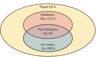
Figure S1: QCA Venn diagram. QCA compatible with both the six-vertex model and the Goldilocks constraint are free-fermionic.

II.3 Goldilocks quantum cellular automata mapped to by the six-vertex model

We now specify the vertex weights under which the six-vertex model maps onto Goldilocks QCA. As a reminder, a Goldilocks QCA effects the neighborhood gate $\hat{u}_{j}$ of Eq. (2), subject to the constraint $f_{\rm G}(m,n)=m\oplus n$ [Eq. (3)]. According to the constraint, the identity operator acts on a target qubit if the neighbors are in $\ket{00}$ or $\ket{11}$. This rule fixes $\hat{V}_{\rm 6V}(0,0)=\hat{V}_{\rm 6V}(1,1)=\hat{\mathbbm{1}}$. Hence, by Eqs. (SII.22)–(SII.31),

$$a_{1}=a_{2}\omega_{2}\omega_{4}=a_{2}\omega_{1}\omega_{3}=1.$$ (SII.33)

If the neighboring spins are in $\ket{01}$ or $\ket{10}$, the target evolves under $\hat{V}$. This rule fixes the remaining vertices’ weights via the matrix equation $\hat{V}_{\rm 6V}(0,1)=\hat{V}_{\rm 6V}(1,0)=\hat{V}$. That matrix equation consists of four components:

$$\bra{0}\hat{V}\ket{0} =c_{1}\omega_{1}=c_{2}\omega_{3},$$ (SII.34)

$$\bra{0}\hat{V}\ket{1} =b_{2}\omega_{3}\omega_{4}=b_{1}\omega_{1}\omega_{4},$$ (SII.35)

$$\bra{1}\hat{V}\ket{0} =b_{1}\omega_{2}\omega_{3}=b_{2}\omega_{1}\omega_{2},\;\>\text{and}$$ (SII.36)

$$\bra{1}\hat{V}\ket{1} =c_{1}/\omega_{1}=c_{2}/\omega_{3}.$$ (SII.37)

To simplify notation, we use Eq. (SII.33) to define $\epsilon_{1}\equiv\omega_{2}\omega_{4}=\omega_{1}\omega_{3}=\pm 1$. Equations (SII.34) and (SII.37) imply $(\omega_{3})^{2}=(\omega_{1})^{2}\equiv\epsilon_{2}$. Combining these two statements yields $\epsilon_{2}=\pm 1$. We can now express some of the original weights (some of the $a$, $b$, and $c$ numbers) in terms of $\epsilon_{1}$, $\epsilon_{2}$, and the other original weights:

$$a_{1}=\epsilon_{1}a_{2}=1\,,\qquad b_{1}=\epsilon_{1}\epsilon_{2}b_{2}\,,\qquad\text{and}\qquad c_{1}=\epsilon_{1}\epsilon_{2}c_{2}\,.$$ (SII.38)

Hence the single-site Goldilocks gate realizable with the six-vertex model has the form

$$\hat{V}=\left(\begin{array}[]{cc}c_{1}\omega_{1}&b_{1}\omega_{1}/\omega_{2}\epsilon_{1}\\ b_{1}\omega_{1}\omega_{2}\epsilon_{1}\epsilon_{2}&c_{1}/\omega_{1}\end{array}\right)\,.$$ (SII.39)

The gate’s unitarity fixes $|\omega_{2}|^{2}=1$,   $|c_{1}|^{2}+|b_{1}|^{2}=1$,   and   $c_{1}^{*}b_{1}+c_{1}b_{1}^{*}=0$.   Up to a global phase factor in $\hat{V}$, we parameterize $c_{1}\omega_{1}=\cos\alpha$,   $b_{1}\omega_{1}\epsilon_{1}=i\sin\alpha$,   and   $\omega_{2}\epsilon_{2}=-ie^{i\beta}$,   wherein $\alpha,\beta\in\mathbb{R}$. The single-site Goldilocks gate realizable with the six-vertex model acquires the form in the main text’s Eq. (4), which we reproduce here:

$$\hat{V}=\left(\begin{array}[]{cc}\cos\alpha&-\epsilon_{2}e^{-i\beta}\sin\alpha\\ e^{i\beta}\sin\alpha&\epsilon_{2}\cos\alpha\end{array}\right)\,.$$ (SII.40)

For any $\epsilon_{1},\epsilon_{2}=\pm 1$, the Goldilocks-constrained six-vertex model’s weights satisfy

$$a_{1}a_{2}+b_{1}b_{2}-c_{1}c_{2}=\epsilon_{1}+\epsilon_{1}\epsilon_{2}(\omega_{1}i\sin\alpha)^{2}-\epsilon_{1}\epsilon_{2}(\omega_{1}\cos\alpha)^{2}=\epsilon_{1}(1-\sin^{2}-\cos^{2}\alpha)=0\,,$$ (SII.41)

i.e., the free-fermion condition from two subsections ago.

We have shown that the six-vertex model, at free-fermionic points of its parameter space, maps onto certain Goldilocks QCA (Fig. S1). One can run this argument backward, to map these QCA onto the free-fermionic six-vertex model. Hence the model and these QCA are equivalent, in the sense of the footnote near the end of the third paragraph in Sec. II.1.

Appendix III Conserved charges

The main text reports eight conserved charges $\hat{Q}_{i}$, wherein $i=1,\ldots,8$, for the free-fermionic Goldilocks QCA with the gate $V_{\rm free}(\alpha,0,-)$. We found five more charges, but they do not enter the truncated GGE, at least for the tilted-ferromagnet initial conditions. The remaining charges are

$$\hat{Q}_{9} =\tan a\,[[\hat{\sigma}^{x}\hat{\sigma}^{x}]]+[[\hat{\sigma}^{x}\hat{\sigma}^{z}]]+[[\hat{\sigma}^{z}\hat{\sigma}^{x}]]-\tan a\,[[\hat{\sigma}^{z}\hat{\sigma}^{z}]]\,,$$ (SIII.42a)

$$\hat{Q}_{10} =[[\hat{\sigma}^{x}\hat{\sigma}^{y}\hat{\sigma}^{z}]]-[[\hat{\sigma}^{z}\hat{\sigma}^{y}\hat{\sigma}^{x}]]\,,$$ (SIII.42b)

$$\hat{Q}_{11} =[[\hat{\sigma}^{y}]+\tan a\,[[\hat{\sigma}^{x}\hat{\sigma}^{y}\hat{\sigma}^{z}]]+[[\hat{\sigma}^{z}\hat{\sigma}^{y}\hat{\sigma}^{x}]]\,,$$ (SIII.42c)

$$\hat{Q}_{12} =[[\hat{\sigma}^{x}\hat{\sigma}^{x}]]+[[\hat{\sigma}^{z}\hat{\sigma}^{y}\hat{\sigma}^{y}\hat{\sigma}^{z}]]\,,\quad\text{and}$$ (SIII.42d)

$$\hat{Q}_{13} =\tan a\,[[\hat{\sigma}^{x}\hat{\sigma}^{y}\hat{\sigma}^{y}\hat{\sigma}^{x}]]+[[\hat{\sigma}^{x}\hat{\sigma}^{y}\hat{\sigma}^{y}\hat{\sigma}^{z}]]+[[\hat{\sigma}^{z}\hat{\sigma}^{y}\hat{\sigma}^{y}\hat{\sigma}^{x}]]-\tan a\,[[\hat{\sigma}^{z}\hat{\sigma}^{y}\hat{\sigma}^{y}\hat{\sigma}^{z}]]\,.$$ (SIII.42e)

The double-bracket notation represents a sum over even-index sites: $[[\hat{A}^{(1)}\hat{A}^{(2)}\ldots\hat{A}^{(n)}]]\coloneqq\sum_{j=0}^{L/2-1}\hat{A}^{(0)}_{2j}\hat{A}^{(1)}_{2j+1}\ldots\hat{A}^{(n)}_{2j+n}$. We calculate the charges of $U\bm{(}V_{\rm free}(\alpha,\beta,-)\bm{)}$ by applying the local change-of-basis transformation (SI.14) to the 13 charges reported for $U\bm{(}V_{\rm free}(\alpha,0,-)\bm{)}$.

The main text describes nine conserved charges of the Goldilocks QCA with the gate $\hat{V}_{\rm free}(\alpha,0,+)$. The algorithm of Ref. [54] enables symbolic and numerical searches for the charges. We applied the symbolic method for generic $\alpha$; the calculation did not terminate. Therefore, we turned to the numerical method. Using it, we found nine charges with support sizes $\leq 5$, for each of the $\alpha$ values sampled.

Appendix IV Details about numerical computations

In this section, we further detail the efficient numerical simulation of the integrable Goldilocks QCA. As we have shown, the Goldilocks QCA (4) effect free-fermionic Floquet dynamics. The time-step operators $\hat{U}(\hat{V}_{\rm free})$ are Gaussian: they follow from multiplying exponentials of Hamiltonians that are quadratic in fermion operators [Eq. (SI.13)]. Consequently, the dynamics can be simulated efficiently, if the system is initialized in a fermionic Gaussian state [35, 36], as we now review. A state is Gaussian if it satisfies Wick’s theorem [35, 36].

For convenience of numerical implementation, we introduce the Majorana operators

$$\hat{\psi}_{2j+1}=\hat{a}^{\dagger}_{j}+\hat{a}_{j}\,\quad\text{and}\quad\hat{\psi}_{2j}=i(\hat{a}_{j}-\hat{a}^{\dagger}_{j})\,,$$ (SIV.43)

so that $\{\hat{\psi}_{a},\hat{\psi}_{b}\}=2\delta_{a,b}$. Each Gaussian state is completely fixed by the covariance matrix

$$C_{ab}(\rho)=\frac{i}{2}\operatorname{tr}\left(\rho\left[\hat{\psi}_{a},\hat{\psi}_{b}\right]\right)\,,$$ (SIV.44)

a $2L\times 2L$ real, skew-symmetric matrix. Upon beginning in a Gaussian initial condition $\ket{\Psi_{0}}$, the state remains Gaussian at all times; its covariance matrix can be computed efficiently. Indeed, consider a Gaussian state $\ket{\Psi_{t}}$ specified by a covariance matrix $C_{t}$. Suppose that we want to update the state with a bilinear unitary

$$\hat{\mathcal{O}}=\exp\left(-\frac{1}{4}\sum_{m,n}K_{m,n}\hat{\psi}_{m}\,\hat{\psi}_{n}\right)\,,$$ (SIV.45)

wherein $K_{m,n}\in\mathbb{R}$ is real and skew-symmetric. By the Baker-Campbell-Haussdorf formula and the Majorana anticommutation relations, $\hat{\mathcal{O}}\ket{\Psi_{t}}$ has the covariance matrix $C_{t+1}=OC_{t}O^{T}$ specified by the $2L\times 2L$ matrix $O=\exp(K)\,.$ $K$ is the matrix with elements $K_{m,n}$, as in (SIV.45). $\hat{\mathcal{O}}$ is a $2^{L}\times 2^{L}$ unitary operator, whereas $O$ is a $2L\times 2L$ orthogonal matrix. Therefore, to classically simulate the time evolution, one must only calculate exponentials and products of matrices whose dimensionalities scale linearly with the system size. Hence the whole algorithm is efficient.

To apply this procedure to our problem, we rewrite the Hamiltonians (7) and (8) in terms of the Majorana operators:

$$\hat{H}_{1}(q)=i\,\frac{\alpha}{2}\,\sum_{j=0}^{L/2-1}\hat{\psi}_{4j+2q}\hat{\psi}_{4j+2q+1}\,,\quad\text{and}\quad\hat{H}_{2}=i\,\frac{\pi}{4}\,\sum_{j=0}^{L-1}(-1)^{j+1}\hat{\psi}_{2j}\hat{\psi}_{2j+3}\,.$$ (SIV.46)

We have assumed that the boundary conditions are periodic. $\hat{H}_{2}$ may require a specific boundary term depending on the desired initial and boundary conditions [37, 38]. Finally, one must specify the initial state’s covariance matrix. In our numerical simulations, the initial state is the fermionic vacuum state $\ket{\Omega}$ (which is a Gaussian state and has definite fermion-number-parity). This state is defined by the condition $a_{j}\ket{\Omega}=0$ for all $j=0,1,\ldots,L-1$. In qubit language, $\hat{\sigma}^{y}_{j}\ket{\Omega}=\ket{\Omega}$ for all $j$:

$$\ket{\Omega}=\left(\frac{\ket{0}+i\ket{1}}{\sqrt{2}}\right)^{\otimes L}\,.$$ (SIV.47)

Recall the covariance-matrix definition (SIV.44) and the relationship between fermionic and Majorana operators. Using these inputs, one can compute the covariance matrix immediately: $C_{ab}(\ket{\Omega}\bra{\Omega})=\delta_{a-1,b}-\delta_{a+1,b}\,.$

Appendix V Single-charge generalized Gibbs ensemble

This section reports analytic results concerning the GGE $\hat{\rho}=e^{-\mu\hat{Q}_{1}}/Z$ that accounts for the conservation of $\hat{Q}_{1}=\sum^{L-1}_{j=0}\hat{\sigma}_{j}\hat{\sigma}_{j+1}$ alone. We compute the partition function $Z=\mathrm{Tr}(e^{-\mu\hat{Q}_{1}})$, chemical potential $\mu$, and $z$-type expectation values $\mathrm{Tr}(\hat{\rho}[\hat{\sigma}^{z}]^{\otimes k})$. We use the computational basis, defined through $\hat{\sigma}^{z}_{j}\ket{m_{j}}=z_{m_{j}}\ket{m_{j}}$, wherein $j=0,\ldots,L-1$,   $m_{j}\in\{0,1\}$,   $z_{0}=1$,   and $z_{1}=-1$.

Define the transfer matrix $P$ with elements $\bra{m_{j}}P\ket{m_{j+1}}$:

$$P=\left(\begin{array}[]{cc}e^{-\mu}&e^{\mu}\\ e^{\mu}&e^{-\mu}\end{array}\right)\,.$$ (SV.48)

The eigenvalues of $P$ are $\lambda_{+}=2\cosh\mu$ and $\lambda_{-}=-2\sinh\mu$. We introduce $P$ to represent the partition function as $Z=\mathrm{Tr}(e^{-\mu\hat{Q}_{1}})=\mathrm{Tr}(P^{L})=\lambda_{+}^{L}+\lambda_{-}^{L}$. The chemical potential is set by the initial condition, here the tilted ferromagnet $\ket{\Psi_{0}}=\ket{\Psi(\theta,\phi)}$. In the thermodynamic limit, one expects,

$$\lim_{L\to\infty}\bra{\Psi_{0}}\hat{Q}_{1}\ket{\Psi_{0}}=\lim_{L\to\infty}\mathrm{Tr}{\bm{(}}\hat{\rho}\hat{Q}_{1}\bm{)}\,.$$ (SV.49)

Since $\ket{\Psi_{0}}$ is translationally invariant, $\bra{\Psi_{0}}\hat{Q}_{1}\ket{\Psi_{0}}=L\bra{\Psi_{0}}\hat{\sigma}^{z}_{0}\hat{\sigma}^{z}_{1}\ket{\Psi_{0}}=L\cos^{2}\theta$. Similarly, $\mathrm{Tr}(\hat{\rho}\hat{Q}_{1})=L\mathrm{Tr}(\hat{\rho}\hat{\sigma}^{z}_{0}\hat{\sigma}^{z}_{1})$. More generally,

$$\mathrm{Tr}\left(\hat{\rho}[\hat{\sigma}^{z}]^{\otimes k}\right) =\frac{1}{Z}\mathrm{Tr}\left([\hat{\sigma}^{z}P]^{k}P^{L-k}\right)$$ (SV.50)

$$=\frac{1+(-1)^{k}}{2}\left(\frac{\lambda_{+}^{L}\lambda_{-}^{k}+\lambda_{+}^{k}\lambda_{-}^{L}}{\lambda_{+}^{L}+\lambda_{-}^{L}}\right)\left[-2\sinh(2\mu)\right]^{-k/2}\,.$$ (SV.51)

If $k=2$, in the thermodynamic limit (as $L\to\infty$), $\lambda_{+}^{L}\gg\lambda_{-}^{L}$, so $\mathrm{Tr}\left(\hat{\rho}[\hat{\sigma}^{z}]^{\otimes 2}\right)\to-2\sinh^{2}\mu/\sinh 2\mu=-\tanh\mu$. Therefore,

$$\mu=-{\rm arctanh}\left(\cos^{2}\theta\right).$$ (SV.52)

Finally, inserting Eq. (SV.52) into (SV.50), we calculate the GGE prediction for the tilted-ferromagnet initial condition:

$$\mathrm{Tr}\left(\hat{\rho}[\hat{\sigma}^{z}]^{\otimes k}\right)=\left(\frac{1+(-1)^{k}}{2}\right)\left(\frac{\cos^{k}\theta+\cos^{2L-k}\theta}{1+\cos^{2L}\theta}\right)\xrightarrow{\mathit{L\to\infty}}\left(\frac{1+(-1)^{k}}{2}\right)\cos^{k}\theta\,.$$ (SV.53)

The GGE predicts that even-$k$ $z$-type expectation values thermalize to their initial values, while odd-$k$ $z$-type expectation values thermalize to zero.

Here we make one comment on GGE predictions made using all the charges (9). The main text observed in Fig. 2 that, as $k$ increases, the equilibrium values approaches zero. We understand this trend in the Heisenberg picture as follows. Return to expression (10) for expectation values $\mathcal{F}(t;,\gamma,k)$. Consider preparing $\ket{\Psi_{0}}$, evolving it forward in time to $\ket{\Psi_{t}}$, perturbing it with $[\hat{\sigma}^{y}]^{\otimes k}$, and evolving backward in time. The resultant state’s overlap with the initial state, $\ket{\Psi_{0}}$, is $\mathcal{F}$. If the perturbation were absent (if $k$ equaled 0), the overlap would be 1. The larger the perturbation, the more the resultant state should differ from the initial state, so the smaller the overlap should be, consistent with our observations.

Appendix VI Details about level statistics

We computed symmetry-resolved spectral statistics as follows. Denote by $\hat{\Pi}$ the operator that shifts the system by one site (the direction of the shift does not impact the rest of our argument). The Goldilocks dynamics conserve the two-site-shift operator $\hat{\Pi}^{2}$, due to the circuit’s brickwork structure: $[\hat{U}(\hat{V}),\,\hat{\Pi}^{2}]=0$, for all $\hat{V}$. Hence this shift operator is a conserved charge itself—quasimomentum. Not only $\hat{U}$, but also the already known charge $\hat{Q}_{1}$ commutes with $\hat{\Pi}^{2}$: $[U(\hat{V}),\,\hat{Q}_{1}]=0$. Therefore, the two charges share an eigenbasis $\{\ket{\psi_{j}}\}$. Denote the $\hat{Q}_{1}$ eigenvalues by $q_{1}=-L,-L+4,\ldots,L$; and the $\hat{\Pi}^{2}$ eigenvalues, by $e^{4\pi iK/L}$, wherein $K\in 0,1,\ldots,L/2$.

Consider the joint eigenspace, shared by the two charges, labeled by some $q_{1}$ and some $K$. Denote the subspace’s dimensionality by $N$. Define the projector onto this subspace by $\hat{R}=\sum_{j=0}^{N-1}\ket{\psi_{j}}\bra{\psi_{j}}$. (We suppress $q_{1}$ and $K$ labels for notational convenience.) From this projector, we construct the operator $\hat{R}\hat{\Pi}\hat{G}(\hat{V},0)\hat{R}^{\dagger}$. Following [50], we compute the operator’s eigenvalues, $e^{i\phi_{\ell}}$. The quasienergies $\phi_{\ell}$ are indexed by $\ell=1,2\ldots N$. We order the quasienergies such that $\phi_{1}\leq\phi_{2}\leq\ldots\leq\phi_{N}$. Then, we compute the spacings $s_{\ell}\coloneqq\phi_{\ell+1}-\phi_{\ell}$. The smallest ratio of adjacent spacings is $r_{\ell}\coloneqq\min\{s_{\ell},\,s_{\ell-1}\}/\max\{s_{\ell},\,s_{\ell-1}\}$. The main text reports on the probability density $P(r)$ for each of two joint eigenspaces.

Appendix VII Gates with larger supports

An important question is whether our free-fermion mapping can extend to more-general constrained discrete dynamics. For instance, Ref. [8] reported about QCA gates supported on $>3$ qubits. Interesting behavior was attributed to Goldilocks gates supported on five qubits, four of which formed the control set. More generally, we can consider QCA whose local gates act on $d>2$ neighboring qubits, $2s<d$ of which form the control set.

We could not find integrable QCA that had the form (1) and whose gates acted on $>3$ qubits. However, exploiting our previous results, one can easily exhibit slightly more-general constrained models that map onto free fermions. We will construct examples with arbitrary $d\geq 4$ and $s=1$.

Consider the $d$-qubit neighborhood gates

$$\hat{u}_{j} \coloneqq\sum_{m,n=0}^{1}\ket{m}\bra{m}_{j}\otimes\hat{V}_{j+1,\ldots j+d-2}(m,n)\otimes\ket{n}\bra{n}_{j+d-1}\,.$$ (SVII.54)

Qubits $j$ and $j+d-1$ form the control set. However, unlike in Eq. (2), the update operator $\hat{V}(m,n)$ may depend nontrivially on the control qubits’ states. Define the partial-step updates

$$\hat{G}(q)\coloneqq\prod_{x}\hat{u}_{(d-s)x+q}\,,$$ (SVII.55)

assuming that $(s+d)$ divides $L$. The single-step Floquet operator may be defined as

$$\hat{U}\coloneqq\prod_{q=0}^{d-2}\hat{G}(q)\,.$$ (SVII.56)

We find a parametric class of QCA that satisfy Eqs. (SVII.54)–(SVII.56) and that map onto free fermions. The local gates have the form

$$\hat{U}_{j}=\hat{W}^{(1)}_{j+1\ldots,j+d-3}\prod_{m=j}^{j+d-3}[CZ]_{m,m+1}\,\hat{W}^{(2)}_{j+1\ldots,j+d-3}\,.$$ (SVII.57)

$W^{(1)}$ and $W^{(2)}$ denote arbitrary unitary operators mapped onto Gaussian ones via the JW transformation (6). For instance, we can choose

$$\hat{W}^{(a)}_{j+1\ldots,j+d-3}=\exp\left(-i\sum_{{\ell}=j+1}^{j+d-3}c_{\ell}^{(a)}\hat{\sigma}^{y}_{\ell}-i\sum_{\gamma,\delta\in\{x,z\}}\sum_{{\ell}=j+1}^{j+d-4}c_{{\ell},\gamma,\delta}^{(a)}\hat{\sigma}^{\gamma}_{\ell}\hat{\sigma}^{\delta}_{{\ell}+1}\right)\,.$$ (SVII.58)

The $a=1,2$, while $c_{j}^{(a)}$ and $c_{j,\gamma,\delta}^{(a)}$ are arbitrary real parameters. The second sum is over only the Pauli operators $\hat{\sigma}^{x}$ and $\hat{\sigma}^{z}$. The nontrivial part of the evolution operator is $\prod_{j}[CZ]_{j,j+1}$. The JW transformation maps this factor onto a Gaussian operator (SI.9), by Eq. (SI.5). By construction, he individual operators $\hat{W}^{(a)}_{j+1\ldots,j+k-3}$ is also Gaussian. Therefore, the whole Floquet operator $\hat{U}$ [Eq. (SVII.56)] is mapped onto a product of Gaussian operators. Hence $\hat{U}$ is Gaussian.

References

- Delorme [1999] M. Delorme, An introduction to cellular automata: some basic definitions and concepts, in Cellular automata: a parallel model (Springer, 1999) pp. 5–49.
- Wolfram [1983] S. Wolfram, Statistical mechanics of cellular automata, Rev. Mod. Phys. 55, 601 (1983).
- Cook et al. [2004] M. Cook et al., Universality in elementary cellular automata, Complex systems 15, 1 (2004).
- Margolus [1987] N. Margolus, Physics and computation, Ph.D. thesis, Massachusetts Institute of Technology (1987).
- Adler et al. [1995] C. Adler, B. Boghosian, E. G. Flekkøy, N. Margolus, and D. H. Rothman, Simulating three-dimensional hydrodynamics on a cellular automata machine, Journal of Statistical Physics 81, 105 (1995).
- Arrighi [2019] P. Arrighi, An overview of quantum cellular automata, Nat. Comp. 18, 885 (2019).
- Farrelly [2020] T. Farrelly, A review of quantum cellular automata, Quantum 4, 368 (2020).
- Hillberry et al. [2021] L. E. Hillberry, M. T. Jones, D. L. Vargas, P. Rall, N. Yunger Halpern, N. Bao, S. Notarnicola, S. Montangero, and L. D. Carr, Entangled quantum cellular automata, physical complexity, and goldilocks rules, Quantum Sci. Tech. 6, 045017 (2021).
- Jones et al. [2022] E. B. Jones, L. E. Hillberry, M. T. Jones, M. Fasihi, P. Roushan, Z. Jiang, A. Ho, C. Neill, E. Ostby, P. Graf, et al., Small-world complex network generation on a digital quantum processor, Nature comm. 13, 4483 (2022).
- Prosen [2021a] T. Prosen, Many-body quantum chaos and dual-unitarity round-a-faces, Chaos: An Interdisciplinary Journal of Nonlinear Science 31, 093101 (2021a).
- Turner et al. [2018] C. J. Turner, A. A. Michailidis, D. A. Abanin, M. Serbyn, and Z. Papić, Weak ergodicity breaking from quantum many-body scars, Nature Phys. 14, 745 (2018).
- Wang et al. [2024] J.-W. Wang, X.-F. Zhou, G.-C. Guo, and Z.-W. Zhou, Quantum many-body scar models in one-dimensional spin chains, Physical Review B 109, 125102 (2024).
- Daley et al. [2022] A. J. Daley, I. Bloch, C. Kokail, S. Flannigan, N. Pearson, M. Troyer, and P. Zoller, Practical quantum advantage in quantum simulation, Nature 607, 667 (2022).
- Onsager [1944] L. Onsager, Crystal statistics. i. a two-dimensional model with an order-disorder transition, Phys. Rev. 65, 117 (1944).
- Pauling [1935] L. Pauling, The structure and entropy of ice and of other crystals with some randomness of atomic arrangement, Journal of the American Chemical Society 57, 2680 (1935).
- Lieb [1967] E. H. Lieb, Residual entropy of square ice, Phys. Rev. 162, 162 (1967).
- Jordan and Wigner [1928] P. Jordan and E. Wigner, Über das paulische Äquivalenzverbot, Zeitschrift für Physik 47, 631 (1928).
- Bethe [1931] H. Bethe, Zur theorie der metalle: I. eigenwerte und eigenfunktionen der linearen atomkette, Zeitschrift für Physik 71, 205 (1931).
- Yang [1967] C. N. Yang, Some exact results for the many-body problem in one dimension with repulsive delta-function interaction, Phys. Rev. Lett. 19, 1312 (1967).
- Baxter [1972] R. J. Baxter, One-dimensional anisotropic heisenberg chain, Annals of Physics 70, 323 (1972).
- Caux and Mossel [2011] J.-S. Caux and J. Mossel, Remarks on the notion of quantum integrability, Journal of Statistical Mechanics: Theory and Experiment 2011, P02023 (2011).
- Baxter [2008] R. J. Baxter, Exactly solved models in statistical mechanics (Dover Pubns, 2008).
- Retore [2022] A. L. Retore, Introduction to classical and quantum integrability, Journal of Physics A: Mathematical and Theoretical 55, 173001 (2022).
- Bazhanov and Sergeev [2023] V. V. Bazhanov and S. M. Sergeev, An ising-type formulation of the six-vertex model, Nuclear Physics B 986, 116055 (2023).
- Vanicat et al. [2018] M. Vanicat, L. Zadnik, and T. Prosen, Integrable trotterization: Local conservation laws and boundary driving, Phys. Rev. Lett. 121, 030606 (2018).
- Ljubotina et al. [2019] M. Ljubotina, L. Zadnik, and T. Prosen, Ballistic spin transport in a periodically driven integrable quantum system, Phys. Rev. Lett. 122, 150605 (2019).
- Bertini et al. [2019] B. Bertini, P. Kos, and T. Prosen, Exact correlation functions for dual-unitary lattice models in 1+ 1 dimensions, Physical review letters 123, 210601 (2019).
- Medenjak et al. [2020] M. Medenjak, T. Prosen, and L. Zadnik, Rigorous bounds on dynamical response functions and time-translation symmetry breaking, SciPost Phys. 9, 003 (2020).
- Claeys et al. [2022] P. W. Claeys, J. Herzog-Arbeitman, and A. Lamacraft, Correlations and commuting transfer matrices in integrable unitary circuits, SciPost Phys. 12, 007 (2022).
- Vernier et al. [2023] E. Vernier, B. Bertini, G. Giudici, and L. Piroli, Integrable digital quantum simulation: Generalized gibbs ensembles and trotter transitions, Phys. Rev. Lett. 130, 260401 (2023).
- Miao and Vernier [2023] Y. Miao and E. Vernier, Integrable Quantum Circuits from the Star-Triangle Relation, Quantum 7, 1160 (2023).
- Pozsgay [2024] B. Pozsgay, Quantum circuits with free fermions in disguise, arXiv:2402.02984 (2024).
- Vernier et al. [2024] E. Vernier, H.-C. Yeh, L. Piroli, and A. Mitra, Strong zero modes in integrable quantum circuits, arXiv:2401.12305 (2024).
- Terhal and DiVincenzo [2002] B. M. Terhal and D. P. DiVincenzo, Classical simulation of noninteracting-fermion quantum circuits, Phys. Rev. A 65, 032325 (2002).
- Bravyi [2004] S. Bravyi, Lagrangian representation for fermionic linear optics, arXiv preprint quant-ph/0404180 (2004).
- Surace and Tagliacozzo [2022] J. Surace and L. Tagliacozzo, Fermionic Gaussian states: an introduction to numerical approaches, SciPost Phys. Lect. Notes 54, 10.21468/SciPostPhysLectNotes.54 (2022).
- Lieb et al. [1961] E. Lieb, T. Schultz, and D. Mattis, Two soluble models of an antiferromagnetic chain, Annals of Physics 16, 407 (1961).
- Cabrera and Jullien [1987] G. G. Cabrera and R. Jullien, Role of boundary conditions in the finite-size ising model, Phys. Rev. B 35, 7062 (1987).
- Li and Po [2022] K. Li and H. C. Po, Higher-dimensional jordan-wigner transformation and auxiliary majorana fermions, Phys. Rev. B 106, 115109 (2022).
- Note [1] An elegant graph-theoretic solution for Hamiltonians was recently presented [chapman2020characterization]. However, not all Hamiltonians with free-fermionic spectra admit of JW mappings to fermion bilinears [81, alcaraz2020free, elman2021free, chapman2023unified, fendley2023free, 32].
- Note [2] Since other qubits’ states control the application of , the operator’s phase affects the global evolution. Therefore need not be unity. In general, . We set aside this subtlety for now, restricting to .
- Gopalakrishnan and Zakirov [2018] S. Gopalakrishnan and B. Zakirov, Facilitated quantum cellular automata as simple models with non-thermal eigenstates and dynamics, Quantum Science and Technology 3, 044004 (2018).
- Gopalakrishnan [2018] S. Gopalakrishnan, Operator growth and eigenstate entanglement in an interacting integrable floquet system, Phys. Rev. B 98, 060302 (2018).
- Causer et al. [2020] L. Causer, I. Lesanovsky, M. C. Bañuls, and J. P. Garrahan, Dynamics and large deviation transitions of the xor-fredrickson-andersen kinetically constrained model, Phys. Rev. E 102, 052132 (2020).
- [45] See Supplemental Material at [URL will be inserted by publisher] for additional details on the six-vertex mapping, Jordan-Wigner transform, efficient numerical computations, single-charge GGE predictions, level statistics, and free-fermionic gates with larger support.
- Note [3] The more common JW transformation reads . Our choice renders the gates and free fermionic, as needed for our proof. More generally, all the usual results hold under the cyclic replacement (“usual JW”) (“our JW”): , , and . Our JW transformation privileges the -direction, rather than the conventional -direction, due to the in .
- Kadanoff and Wegner [1971] L. P. Kadanoff and F. J. Wegner, Some critical properties of the eight-vertex model, Physical Review B 4, 3989 (1971).
- Wu [1969] F. Y. Wu, Exact solution of a model of an antiferroelectric transition, Physical Review 183, 604 (1969).
- Baxter [1970] R. J. Baxter, Exact isotherm for the model in direct and staggered electric fields, Phys. Rev. B 1, 2199 (1970).
- Prosen [2021b] T. Prosen, Reversible cellular automata as integrable interactions round-a-face: Deterministic, stochastic, and quantized, arXiv 2106.01292 (2021b).
- Gombor and Pozsgay [2021] T. Gombor and B. Pozsgay, Integrable spin chains and cellular automata with medium-range interaction, Phys. Rev. E 104, 054123 (2021).
- Fagotti and Essler [2013] M. Fagotti and F. H. L. Essler, Reduced density matrix after a quantum quench, Phys. Rev. B 87, 245107 (2013).
- Fagotti [2014] M. Fagotti, On conservation laws, relaxation and pre-relaxation after a quantum quench, J. Stat. Mech. 2014, P03016 (2014).
- Prosen [2007] T. Prosen, Chaos and complexity of quantum motion, Journal of Physics A: Mathematical and Theoretical 40, 7881 (2007).
- Note [4] We identify certain equipment to specify the computational procedure adequately. Such identification is not intended to imply recommendation or endorsement of any product or service by NIST; nor is it intended to imply that the software identified is necessarily the best available for the purpose.
- Majidy et al. [2023] S. Majidy, W. F. Braasch Jr, A. Lasek, T. Upadhyaya, A. Kalev, and N. Yunger Halpern, Noncommuting conserved charges in quantum thermodynamics and beyond, Nature Reviews Physics 5, 689 (2023).
- Lostaglio et al. [2017] M. Lostaglio, D. Jennings, and T. Rudolph, Thermodynamic resource theories, non-commutativity and maximum entropy principles, New Journal of Physics 19, 043008 (2017).
- Guryanova et al. [2016] Y. Guryanova, S. Popescu, A. J. Short, R. Silva, and P. Skrzypczyk, Thermodynamics of quantum systems with multiple conserved quantities, Nature Communications 7, 12049 (2016).
- Yunger Halpern et al. [2016] N. Yunger Halpern, P. Faist, J. Oppenheim, and A. Winter, Microcanonical and resource-theoretic derivations of the thermal state of a quantum system with noncommuting charges, Nature Communications 7, 1 (2016).
- Ares et al. [2023] F. Ares, S. Murciano, E. Vernier, and P. Calabrese, Lack of symmetry restoration after a quantum quench: An entanglement asymmetry study, SciPost Phys. 15, 089 (2023).
- Fukai et al. [2020] K. Fukai, Y. Nozawa, K. Kawahara, and T. N. Ikeda, Noncommutative generalized gibbs ensemble in isolated integrable quantum systems, Phys. Rev. Res. 2, 033403 (2020).
- Corps and Relaño [2023] Á. L. Corps and A. Relaño, General theory for discrete symmetry-breaking equilibrium states, arXiv:2303.18020 (2023).
- Potter and Vasseur [2016] A. C. Potter and R. Vasseur, Symmetry constraints on many-body localization, Physical Review B 94, 224206 (2016).
- De Nardis et al. [2021] J. De Nardis, S. Gopalakrishnan, R. Vasseur, and B. Ware, Stability of superdiffusion in nearly integrable spin chains, Physical review letters 127, 057201 (2021).
- Note [5] Reference [51] discusses neither mappings onto free fermions nor the gate (4) with general parameter values.
- Rigol et al. [2008] M. Rigol, V. Dunjko, and M. Olshanii, Thermalization and its mechanism for generic isolated quantum systems, Nature 452, 854 (2008).
- Vidmar and Rigol [2016] L. Vidmar and M. Rigol, Generalized gibbs ensemble in integrable lattice models, J. Stat. Mech. 2016, 064007 (2016).
- Essler and Fagotti [2016] F. H. Essler and M. Fagotti, Quench dynamics and relaxation in isolated integrable quantum spin chains, J. Stat. Mech. 2016, 064002 (2016).
- Pozsgay et al. [2017] B. Pozsgay, E. Vernier, and M. A. Werner, On generalized gibbs ensembles with an infinite set of conserved charges, Journal of Statistical Mechanics: Theory and Experiment 2017, 093103 (2017).
- Note [6] For free fermions, one can compute the full GGE predictions via the quench action method [caux2013time, caux2016quench]. For the few-body expectation values we focus on, sufficiently accurate predictions follow from the more elementary truncated-GGE approach [52].
- Landau and Lifshitz [1980] L. D. Landau and E. M. Lifshitz, Statistical Physics: Part 1 (Butterworth-Heinemann, Oxford, 1980).
- Yunger Halpern et al. [2020] N. Yunger Halpern, M. E. Beverland, and A. Kalev, Noncommuting conserved charges in quantum many-body thermalization, Phys. Rev. E 101, 042117 (2020).
- Kranzl et al. [2023] F. Kranzl, A. Lasek, M. K. Joshi, A. Kalev, R. Blatt, C. F. Roos, and N. Yunger Halpern, Experimental observation of thermalization with noncommuting charges, PRX Quantum 4, 020318 (2023).
- Giraud et al. [2022] O. Giraud, N. Macé, E. Vernier, and F. Alet, Probing symmetries of quantum many-body systems through gap ratio statistics, Phys. Rev. X 12, 011006 (2022).
- Oganesyan and Huse [2007] V. Oganesyan and D. A. Huse, Localization of interacting fermions at high temperature, Phys. Rev. B 75, 155111 (2007).
- Atas et al. [2013] Y. Y. Atas, E. Bogomolny, O. Giraud, and G. Roux, Distribution of the ratio of consecutive level spacings in random matrix ensembles, Phys. Rev. Lett. 110, 084101 (2013).
- Berry and Tabor [1977] M. V. Berry and M. Tabor, Level clustering in the regular spectrum, Proceedings of the Royal Society of London. A. Mathematical and Physical Sciences 356, 375 (1977).
- Bohigas et al. [1984] O. Bohigas, M. J. Giannoni, and C. Schmit, Characterization of chaotic quantum spectra and universality of level fluctuation laws, Phys. Rev. Lett. 52, 1 (1984).
- Wintermantel et al. [2020] T. M. Wintermantel, Y. Wang, G. Lochead, S. Shevate, G. K. Brennen, and S. Whitlock, Unitary and nonunitary quantum cellular automata with rydberg arrays, Phys. Rev. Lett. 124, 070503 (2020).
- Sá et al. [2021] L. Sá, P. Ribeiro, and T. Prosen, Integrable nonunitary open quantum circuits, Phys. Rev. B 103, 115132 (2021).
- Fendley [2019] P. Fendley, Free fermions in disguise, J. Phys. A: Math. Theor. 52, 335002 (2019).
- Note [7] One might hesitate to label as equivalent two models that have different numbers of allowed configurations. These different numbers, however, merely distinguish one model’s partition function from the other model’s by a factor of two [48]. Hence the term equivalent appears in [48].