Information Theory and Direction Selectivity

Information Theory and Direction Selectivity

Abstract

In this brief paper, the authors study the tuning curves of starburst amacrine cells (SACs) and introduce a quantity called the irresolution or ambiguity of a SAC. They show that the rate of data generated by a starburst amacrine cell is inversely proportional to its irresolution. This is done by providing bounds on the rate required to encode the generated data. This technique can be applied to different cell types with different tuning curves. In this manner, information theoretic views can be introduced to the cases of biological cells which are not normally considered as transmitters of information as say retinal ganglion cells are. The intuition that even such cells generate information is thus quantified.

The detection of motion is a need of living organisms. In the wakeful state of consciousness, things are not necessarily still. Motion may only be detected against a background stillness. Therefore to identify motion, more than a single cell may be needed. In the retina, this is therefore one of the earliest places where co-operation and co-ordination between cells is needed.

There are two main known mechanisms for direction selectivity: The Reichardt detector, shown conceptually in Figure 1 and the Rall mechanism, Figure 2.

Figure 1: Reichardt detector

The Reichardt detector works as follows. The bipolar cells A and B impinge on the dendrite under consideration at locations A and B, respectively. The input of bipolar cell A is broad, while that of bipolar cell B is narrower. Suppose the stimulus moves from left to right. Then, first the broad peak is stimulated and then the narrower peak. When these peaks reach the terminal, they get summed. The narrower then gets raised by the broad and they together cross the threshold. Suppose the stimulus moves from right to left. Then, first the narrower peak is stimulated and then the broader one. As a result, there is little or no overlap between the two peaks, and even if summed, they will not cross the threshold. This is what gives rise to direction selectivity.

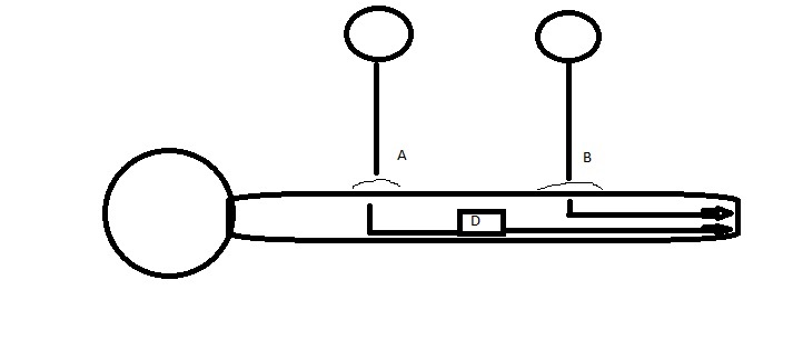
Figure 2: Rall mechanism

In the Rall mechanism there is a delay element, D, introduced by the axoplasm between A and B. This delay causes the signals from A to be broadened when reaching the terminal, whereas the signals from B remain narrow. A similar summation effect as the Reichardt mechanism then leads to directional preference.

The Rall and the Reichardt mechanisms have been known for some time. Several experiments have tried to discriminate between the two mechanisms, to pick the correct one. The predicted observations for the Reichardt mechanism are found to match more closely the experimental results than those of the Rall mechanism.

From the theorists perspective, can we consider the dendrite as a channel? Alternately, it is a source encoder. The question is, what is it that qualifies an encoder as being good. And if a dendrite is a communication channel, what is the capacity of the channel? Does there lurk a rate-distortion problem? From the experimenter’s perspective, the stimulus is presented on the screen and an output is obtained from the apex of the dendrite. So it does seem to be a communication channel. Figures 3 and 4 show how the experimentalist observes the output.

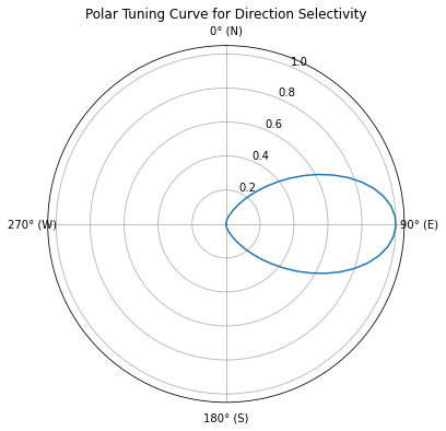
Figure 3: Polar Tuning Curve.

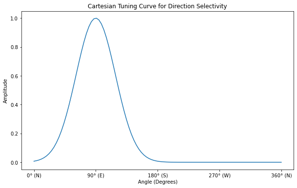
Figure 4: Cartesian version of polar tuning curve.

Consider Figure 5. It shows the response of a starburst amacrine cell to stimulation presented at various input directions. The response is given by the curve $f(\theta)$.

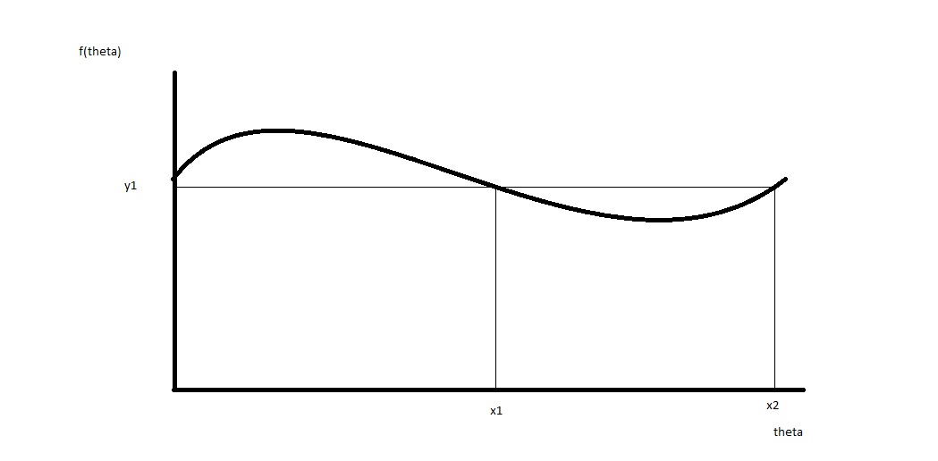
Figure 5: The response of a starburst amacrine cell to different input directions, depicted as an arbitrary function of angle theta. The image y1 corresponds to two preimages x1 and x2.

Suppose the experimenter presents an angle of $\theta_{1}$ degrees. The cell has a response curve $f_{1}(\theta)$ so it produces an amplitude response $f_{1}(\theta_{1})$. This response is corrupted by noise $\eta_{1}$ so that the final output with the experimenter is

$$y_{1}=f_{1}(\theta_{1})+\eta_{1}.$$ (1)

It is the task of the cell, we can assume, to allow the recovery of the direction (in degrees) from $y_{1}$. Here we show that it is impossible to recover the angle uniquely.

Lemma 1.

Recovery Lemma. Given a cellular response $y_{1}$ (see Eqn. 1), it is impossible to recover the directional angle in degrees uniquely, for an arbitrary response function $f_{1}(\cdot)$.

Proof.

To prove this lemma we need to come up with one example of a response function where it is not possible to recover the directional angle uniquely. One such example is shown in Figure 5.∎ ∎

Next we quantify the error in recovery.

Theorem 2.

Given a cellular response $y_{1}$ (see Eqn. 1) and a response function $f_{1}(\cdot)$, the error (representational) in recovering the input direction is bounded from above by $\log_{2}(k)$ bits where $k$ is the maximum number of angles corresponding to a value of the response function. From rudimentary graphical considerations, $k=2*n-1$ where $n$ is the number of critical points (maxima or minima) of the (continuous) response function.

Proof.

Suppose we are using $l$ bits of precision to represent a real number. The cellular response must be used to first estimate the value of the response function $f_{1}(\cdot)$ at the transmitted angle $\theta$, in the presence of Gaussian noise. The error analysis for recovering the value of the response function, would be the same as that for an additive white Gaussian noise channel, which has a probability of error $Poe$ which decays with block length $N$, given by the reliability function:

$$Poe\approx\exp^{-Ng(R,N)}$$ (2)

where

$$g(R,N)=C/2-R$$ (3)

for low rates and

$$g(R,N)=(\sqrt{C}-\sqrt{R})^{2}$$ (4)

for high rates less than capacity [1]. Under this probability of error decay law, the value of the response function can be estimated to within

$$POE\leq\exp^{-lg(R,l)}$$ (5)

at the data rate $R$ bits per second. This means that $l\times R$ bits are transmitted in $l$ seconds. ∎

We have next to recover from the value of the response function, the actual angle that was transmitted and we immediately see that if there are at most $k$ angles corresponding to the estimated value of the response function, then $\log_{2}(k)$ bits would suffice to recover the precise angle.

Definition 3.

Irresolution

As per Theorem 2 a total of $s$ bits must be transmitted by the cell for every $l$ seconds of directional information transmission, where $l\times R\leq s\leq l\times R+\log_{2}(k)$. We send $c=s/(l*R)$ bits for every input bit. $c$ is thus dimensionless. Clearly, $1\leq c\leq 1+\frac{\log_{2}(k)}{l*R}$. Since this allows error free recovery, this number is akin to a performance metric for the system. We can call it the irresolution of the cell. Clearly, if irresolution increases for a change in coding mechanism (Rall, Reichardt, etc.), the new mechanism is taking fewer bits in for every output bit and so is less effective in resolving the input angle. This allows us to quantify potential coding mechanisms’ performance by simply looking at the response function. ∎

This definition is explored in Figure 6. The irresolution goes down as the transmission duration increases. The curves look like rate-distortion functions. We will explore this parallel shortly.

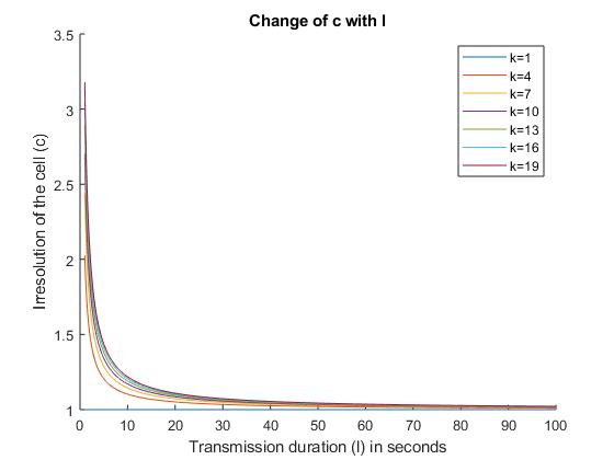
Figure 6: Variation in the irresolution of a cell with increasing duration of transmission and varying directional ambiguity $k$

We can ask the question, which coding scheme is optimal for transmitting in the presence of irresolution. We can also allow different mechanisms to send the image and the preimage resolving bits and compare the resulting achieved bit rates with a biophysically plausible cellular mechanism such as the Rall or Reichardt mechanisms discussed above. The irresolution of the cell is akin to a distortion and we can plot, on the horizontal-axis, the rate instead of the duration of transmission. This is shown in Fig. 7.

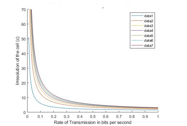
Figure 7: Irresolution-rate formulation: Bound on the irresolution of a cell with increasing rate of transmission (and a total transmission duration of 2 seconds) and varying directional ambiguity $k$. In the legend, $k$ goes from 2 through 20 in steps of 3.

To conclude, in this paper we introduced a simple information theoretic analysis of the tuning curve generated by a starburst amacrine cell. We introduced a new quantity called the irresolution of a cell and provided illustrations of how it varies with directional ambiguity, a parameter we defined: $k$.

References

- [1] Robert G Gallager. Information theory and reliable communication, volume 588. New York: Wiley, 1968.