Electron-Phonon Coupling using Many-Body Perturbation Theory:
Implementation in the Questaal Electronic Structure Suite

Abstract

The ability to calculate the electron-phonon coupling (e-ph ) from first principles is of tremendous interest in materials science, as it provides a non-empirical approach to understand and predict a wide range of phenomena. While this has largely been accomplished in the Kohn-Sham framework of density functional theory (KS-DFT), it is becoming more apparent that standard approximations in KS-DFT can be inaccurate. These discrepancies are often attributed to a non-local potential where more advanced approaches to DFT or many-body perturbation theory have been used. However, a highly reliable and efficient first-principles approach to compute these quantities is still missing. With the goal of realizing a high-fidelity description of e-ph , we present a new field-theoretical methodology, incorporating the seminal work of Baym and Hedin within the quasiparticle self-consistent GW (QSGW) approximation, and the Questaal electronic structure package.

I Introduction

The interaction between electrons and a vibrating lattice (phonons) gives rise to a wide variety of physical properties of materials. A partial list includes: determining the temperature dependence of the electrical transport coefficients in metals and semiconductors Pizzi et al. (2014); enabling optical transitions in indirect-gap semiconductors Noffsinger et al. (2012); renormalization of the effective mass of charge carriers; playing a central role the thermalization of hot carriers that can critically affect the performance of electronic, optoelectronic, photovoltaic, and plasmonic devices Sjakste et al. (2007). The e-ph also determines the lifetimes of electron spin in perfect crystals or at defect sites Gao et al. (1998) which is of importance to spintronics and quantum information. In conventional superconductors, the e-ph drives the formation of Cooper pairs in a condensate, while in unconventional superconductors (such as copper oxides) the role of the e-ph is still actively debated Chen et al. (2021).

Owing to its vital importance in so many phenomena, the ability to determine the e-ph reliably and accurately is of considerable interest in numerous science disciplines, such as physics, chemistry, electrical engineering, materials science, and mechanical engineering. The first ab initio framework to calculate e-ph used a Kohn-Sham implementation Kohn and Sham (1965) of density functional theory Hohenberg and Kohn (1964) (KS-DFT), originated in the early 1990’s Baroni et al. (1987); Gonze et al. (1992); Savrasov (1992). The Kohn-Sham approach continues to be the predominant method to calculate e-ph and lattice-related properties Dacorogna et al. (1985); Gonze and Lee (1997) usually using the local density approximation (LDA) or the generalized gradient approximation (GGA) for the exchange-correlation potential. These methods use density-functional perturbation theory (DFPT), a perturbative approach within KS-DFT. It is an efficient way to calculate phonon modes at any wave vector in the Brillouin zone (BZ) of the material and the electron-phonon matrix elements that couple two Kohn-Sham electronic states. DFPT is universally applicable, but it has become apparent that the electron-phonon coupling strength is often significantly underestimated Shang and Yang (2023). Part of the error originates from the fact that Kohn-Sham states originate from a fictitious auxiliary Hamiltonian. Direct comparison with experiments is not rigorous nor does its potential have knowledge of non-local correlations. As is well known, DFT bandgaps are usually underestimated, and the origin can be traced at least in part to the local potential Grüning et al. (2006). It seems likely that much of the discrepancies found in DFPT have a similar origin.

Standard KS-DFT functionals often rather poorly describe the electron-phonon coupling even in simple sp-bonded compounds such as graphene and diamond. In graphene and graphite, Lazzeri et al. Lazzeri et al. (2008) showed an increase of $\sim 40\%$ in the intraband electron-phonon matrix element and better phonon dispersion at the $K$ point by using a non-local $GW$ self-energy over the local Kohn-Sham potential. For diamond, Antonius et al.Antonius et al. (2014) showed a ${\sim}40\%$ increase over the standard KS-DFT result in the renormalized band gap due to the zero-point motion of the lattice. Developments with hybrid functionals showed an enhancement in the e-ph of roughly three times in superconducting bismuthate Ba_1-xK_xBiO₃  Li et al. (2023) predicting a critical temperature of 31 K, agreeing quite well with the experimental value of 32 K. Similar results were also obtained from using the GW band structure Li et al. (2019). It is perhaps not surprising that extensions to pure DFT (where the potential is the same for all electrons) improve on the result. Hybrid functionals mimic GW with empirical nonlocal additions to DFT. While such approaches Li et al. (2023) or many-body theory within the GW approximation Li et al. (2019) have been used to describe e-ph for materials where non-local correlations in the self-energy are important, a highly reliable, systematic, and efficient first-principles approach to compute these quantities is still missing.

In this paper, we aim at building a new field-theoretical methodology able to predict electronic quasiparticles and their interactions with lattice vibrations using Green’s functions as the foundation. In Section II, we outline the formal theory that will be used. An overview of the vibrating crystal in the Born-Oppenheimer and harmonic approximation in II.1. Following the work and general notation presented in Ref. Giustino (2017), we summarize the Green’s function treatment of the coupled electron-phonon system in Section II.2. Here, we cast the e-ph as the matrix element of the gradient of the screened Coulomb interaction as opposed to its counterpart using DFPT. Finally, in II.3, we give an overview of the self-consistent $GW$ approximation used in the Questaal electronic structure suite. In Section III, we discuss the formal implementation using Questaal’s optimized LMTO basis function in conjunction with the mixed product basis for efficient computation of many-body quantities including excitonic effects. In Section IV, we introduce the details of the computation of the e-ph matrix elements in the Questaal electronic structure suite, and some advanced technical details are presented in Sections V and VI. In Section VII, we delve into the formalism and challenges associated with computing the dynamical matrix within a field-theoretic approach. Finally, in Section VIII we present a comprehensive testing of the implemented field-theoretic framework, comparing our numerical results with experimentally derived Fermi surface-averaged electron-phonon matrix elements for the highest optical phonon branch and Kohn anomalies in graphene.

II Theory

In this section, we provide an overview of the fundamental formalism employed in the computation of e-ph interaction within a field-theoretic approach. We begin by introducing the Hamiltonian of the vibrating crystal within the Born-Oppenheimer restriction of the adiabatic approximation from potential energy surfaces obtained from integrating out the electrons. Subsequently, we provide a succinct derivation and summary of the established field-theoretic method for computing the e-ph matrix elements originally presented in reference Hedin (1965); Baym (1961) using the convention of the modern review in reference Giustino (2017). In this framework, electrons and phonons are not treated as distinct subsystems but allows a comprehensive theoretical framework for addressing the coupling between electrons and phonons which is presented in Sec. II.2. It is important to mention that a new framework of the coupled electron-phonon system has been proposed Stefanucci et al. (2023), however its difficulty in handling extended systems is a conceptual issue that we cannot address here, so we will leave its contents for another publication.

II.1 Lattice vibration in crystals

Lattice dynamics in crystals is extensively discussed by several authors Born and Huang (1954); Ziman (1960); Kittel (1963, 1976); Ashcroft and Mermin (1976); Maradudin (1971), but for this paper, we introduce the notation that will prove beneficial for forthcoming discussions and provide a summary of relevant aspects for the remaining sections of this paper. To do so, we consider a system comprising $M$ nuclei within the unit cell, each with mass $m_{r}$ and charge $Z_{r}e$ which are claimed to have an equilibrium configuration $\{\bm{\tau}^{0}_{rl}\}$. The out of equilibrium nuclear vector position of the $r$-th atom within the unit cell and its corresponding Cartesian coordinates are denoted by $\bm{\tau}_{r}$ and $\tau_{r\alpha}$, respectively. To describe the infinitely extended solid, we apply the Born-von Karman (BvK) boundary conditions, where periodic boundary conditions are imposed on a large supercell containing $N_{\mathbf{k}}$ unit cells, identified by the direct lattice vectors $\mathbf{R}_{l}$, with $l$ ranging from 1 to $N_{\mathbf{k}}$. Therefore, the Cartesian coordinates of the $r$-th nucleus belonging to the $l$-th unit cell is defined as $\bm{\tau}_{rl}=\bm{\tau}_{r}+\mathbf{R}_{l}$.

Investigating lattice vibrations requires the total potential energy stemming from systems of interacting electrons and nuclei within the BvK supercell and denoted as $U(\{\bm{\tau}_{rl}\})$ (the braces are a short-hand notation for the coordinates of all the ions). The total potential energy accounts for electrons in their ground state, while nuclei are treated as classical particles fixed at coordinates $\bm{\tau}_{rl}$. The analysis begins with the harmonic approximation, wherein the total potential energy is expanded to second order in the ionic displacements $\Delta\bm{\tau}_{rl}$ in the BvK supercell away from their equilibrium positions $\bm{\tau}^{0}_{rl}$

$$U(\{\bm{\tau}_{rl}\}) \approx U_{0}+\tfrac{1}{2}\sum_{r\alpha l}\sum_{s\beta t}\frac{\partial^{2}U(\{\bm{\tau}_{rl}\})}{\partial\tau_{r\alpha l}\partial\tau_{s\beta t}}\mathinner{\langle{\Delta\hat{\tau}_{r\alpha l}}\rangle}\mathinner{\langle{\Delta\hat{\tau}_{s\beta t}}\rangle}$$

$$= U_{0}+\tfrac{1}{2}\sum_{r\alpha l}\sum_{s\beta t}C_{rs}^{\alpha\beta}(\mathbf{R}_{l},\mathbf{R}_{t})\mathinner{\langle{\Delta\hat{\tau}_{r\alpha l}}\rangle}\mathinner{\langle{\Delta\hat{\tau}_{s\beta t}}\rangle}.$$

$U_{0}$ denotes the total potential energy evaluated for the ions in their equilibrium positions, and $\{C_{rs}^{\alpha\beta}(\mathbf{R}_{l},\mathbf{R}_{p})\}$ is the set of interatomic force constants (IFCs )

$$C_{rs}^{\alpha\beta}(\mathbf{R}_{l},\mathbf{R}_{t})=\frac{\partial^{2}U(\{\bm{\tau}_{rl}\})}{\partial\tau_{r\alpha l}\partial\tau_{s\beta t}}$$ (2)

with $\alpha$ and $\beta$ denoting Cartesian coordinates and $r$ and $s$ labeling atoms in the unit cell, and where the derivatives are evaluated at the equilibrium lattice configuration. The ionic displacements $\mathinner{\langle{\Delta\hat{\bm{\tau}}_{rl}}\rangle}$ are defined as

$$\bm{\tau}_{rl} = \bm{\tau}_{rl}^{0}+\mathinner{\langle{\Delta\hat{\bm{\tau}}_{rl}}\rangle}$$ (3)

$$= \bm{\tau}_{r}^{0}+\mathbf{R}_{l}+\mathinner{\langle{\Delta\hat{\bm{\tau}}_{rl}}\rangle}\quad\quad l=1,\dots,N_{\mathbf{k}}\,.$$

and correspond to the expectation value of the nuclear displacement operator

$$\Delta\hat{\mathbf{\tau}}_{r\alpha l}=\frac{1}{\sqrt{N_{\mathbf{q}}}}\sum_{\mathbf{q}\nu}\biggl{(}\frac{\hbar}{2m_{r}\omega_{\mathbf{q}\nu}}\biggr{)}^{1/2}e^{i\mathbf{q}\cdot\mathbf{R}_{l}}e_{r\alpha,\nu}(\mathbf{q})\bigl{(}\hat{a}_{\mathbf{q}\nu}+\hat{a}^{\dagger}_{-\mathbf{q}\nu}\bigr{)}\,.$$ (4)

In Equation (4), $m_{r}$ stands for the mass of the $r$-th nucleus in the unit cell, $\hat{a}^{\dagger}_{\mathbf{q}\nu}$ and $\hat{a}_{\mathbf{q}\nu}$ are the standard creation and destruction operators, respectively, defined for each phonon of energy $\hbar\omega_{\mathbf{q}\nu}$ and polarization $e_{r\alpha,\nu}(\mathbf{q})$ for a given $\nu$-th phonon mode and phonon wave vector $\mathbf{q}$. These operators are introduced to conveniently describe the nuclear dynamics in terms of quanta of lattice vibrations, i.e. the phonons, and obey the commutation relations

$$[\hat{a}_{\mathbf{q}\nu},\hat{a}^{\dagger}_{\mathbf{q}^{\prime}\nu^{\prime}}]=\delta_{\nu\nu^{\prime}}\delta_{\mathbf{q},\mathbf{q}^{\prime}}$$

$$[\hat{a}_{\mathbf{q}\nu},\hat{a}_{\mathbf{q}^{\prime}\nu^{\prime}}]=[\hat{a}^{\dagger}_{\mathbf{q}\nu},\hat{a}^{\dagger}_{\mathbf{q}^{\prime}\nu^{\prime}}]=0\,,$$ (5)

showing that the quanta of the harmonic oscillators in crystals obey Bose-Einstein statistics. The orthonormal polarization vectors $\mathbf{e}_{r,\nu}(\mathbf{q})$ and the phonon frequencies $\omega_{\mathbf{q}\nu}$ are the eigenvectors and the square root of the eigenvalues of the Hermitian dynamical matrix $D^{\alpha\beta}_{rs}(\mathbf{q})$, respectively, defined as

$$D_{rs}^{\alpha\beta}(\mathbf{q})=\frac{1}{\sqrt{m_{r}m_{s}}}\sum_{p}C_{rs}^{\alpha\beta}(0,\mathbf{R}_{p})e^{i\mathbf{q}\cdot\mathbf{R}_{p}}\,,$$ (6)

i.e. as Bloch transform of the IFCs $C_{rs}^{\alpha\beta}(\mathbf{R}_{l},\mathbf{R}_{p})$. The phonon wave vectors $\mathbf{q}$ and electronic wave vectors $\mathbf{k}$ are selected to originate from uniform and unshifted commensurate grids, each containing $N_{\mathbf{q}}$ and $N_{\mathbf{k}}$ points, respectively. This choice is motivated by the observation that, even when the $\mathbf{k}$ vector is restricted to the irreducible wedge, $\mathbf{k}+\mathbf{q}$ always spans the whole BZ.

By combining Eqs. (II.1) and (2) we can define the Hamiltonian for nuclei considered as quantum particles

$$\hat{H}_{n}=\hat{T}_{n}+\tfrac{1}{2}\sum_{r\alpha l}\sum_{s\beta t}C_{rs}^{\alpha\beta}(\mathbf{R}_{l},\mathbf{R}_{t})\mathinner{\langle{\Delta\hat{\tau}_{r\alpha l}}\rangle}\mathinner{\langle{\Delta\hat{\tau}_{s\beta t}}\rangle}$$ (7)

where the nuclear kinetic energy operator $\hat{T}_{n}$ is evaluated as

$$\hat{T}_{n}=-\sum_{r\alpha l}\frac{\hbar^{2}}{2m_{r}}\frac{\partial^{2}}{\partial\tau_{r\alpha l}^{2}}\,.$$ (8)

The Hamiltonian in Eq. (7) relies on (i) the harmonic approximation, i.e. the truncation of the Taylor expansion of the total potential energy (II.1) to second order in the nuclear displacements, and (ii) the Born-Oppenheimer adiabatic approximationBorn and Oppenheimer when the IFCs (2) are evaluated with the electrons in their ground state. Furthermore, by combining Eqs. (2)-(8) we can rewrite the nuclear Hamiltonian (7) in terms of $3MN_{\mathbf{q}}$ independent harmonic oscillators

$$\hat{H}_{n}=\sum_{\mathbf{q}\nu}\hbar\omega_{\mathbf{q}\nu}(\hat{a}^{\dagger}_{\mathbf{q}\nu}\hat{a}_{\mathbf{q}\nu}+\tfrac{1}{2})\,,$$ (9)

whose ground-state nuclear wave function is the product of Gaussians and all additional states can be generated by applying the operators $\hat{a}^{\dagger}_{\mathbf{q}\nu}$ to the ground state. In the case $\lvert{\mathbf{q}}\rvert=0$ solving the eigenvalue problem for the dynamical matrix (6) provides three acoustic normal modes corresponding to the translation of the entire crystal and for which $\omega_{\mathbf{q}\nu}=0$. For these modes the expectation value of the nuclear displacement operator (4) is ill defined in the long wavelength limit, which could pose a limitation on the modeling of the e-ph coupling. However, acoustic sum-rules impose that the e-ph matrix elements corresponding to acoustic phonon modes in the long wavelength limit are identically zero, rendering them unnecessary for consideration in the numerical solution of expressions involving summations over all the phonon modes and the entire BZ.

We conclude this section by briefly discussing possible approaches that can be employed for computing the IFCs . The most widely used first-principles method is based on DFPT Baroni et al. (1987); Gonze et al. (1992); Savrasov (1992), where a Sternheimer equationSternheimer (1954) for the first order lattice-periodic variation $\partial_{r\alpha,\mathbf{q}}v^{\text{KS}}$ of the mean-field local Kohn-Sham (KS) potential is solved with the aim to evaluate Eq. (2). This approach circumnavigates the main disadvantage of frozen-phonon algorithms where supercells may become impractically large when evaluating dynamical matrix elements (6) corresponding to long-wavelength phonons. In addition to the DFPT method, an alternative approach exists for computing the screened perturbation $\partial_{r\alpha,\mathbf{q}}v^{\text{KS}}$ known as the dielectric approach Pick et al. (1970); Quong and Klein (1992). While this method has not been as widely adopted as DFPT, it serves as a valuable means to bridge DFT calculations of phonon dispersions and electron-phonon matrix elements within the field-theoretic formulation outlined in Section II.2. The IFCs can be obtained by deriving the key expression of the dielectric approach starting from DFPT: within this formalism the first order lattice-periodic variation $\partial_{r\alpha,\mathbf{q}}n$ of the total electron density is related to the the first order variation $\partial_{r\alpha,\mathbf{q}}v^{\text{KS}}$ of the KS potential by means of the expression

$$\partial_{r\alpha,\mathbf{q}}n(\mathbf{r})=\int_{\Omega_{0}}d\mathbf{r}^{\prime}\chi^{\mathbf{q}}_{0}(\mathbf{r},\mathbf{r}^{\prime})\partial_{r\alpha,\mathbf{q}}v^{\text{KS}}(\mathbf{r}^{\prime})\,,$$ (10)

where $\chi_{0}^{\mathbf{q}}$ is the lattice-periodic independent particle electron polarizability projected over the phonon wave vector $\mathbf{q}$ within the BZ. Alternately, one can make use of the field-theoretic approach outlined in Sec. II.2.2. Nevertheless, both the dielectric and field-theoretic approaches converge to the same expression for the IFCs within the harmonic and adiabatic approximations

$$C^{\alpha\beta}_{rs}(\mathbf{R}_{l},\mathbf{R}_{l^{\prime}})=\sum_{tn}\biggl{(}\delta_{ln}\delta_{rt}-\delta_{ll^{\prime}}\delta_{rs}\biggr{)}\int_{\Omega}\int_{\Omega}\int_{\Omega}\partial_{r\beta}V^{(0)}_{sl^{\prime}}(\mathbf{r})v^{-1}(\mathbf{r}-\mathbf{r}_{1})\varepsilon^{-1}_{e,\text{DFT}}(\mathbf{r}_{1},\mathbf{r}_{2})\partial_{r_{2}\alpha}V^{(0)}_{tn}(\mathbf{r}_{2})\,d\mathbf{r}\,d\mathbf{r}_{1}\,d\mathbf{r}_{2}\,,$$ (11)

where $\varepsilon^{-1}_{e,\text{DFT}}(\mathbf{r}_{1},\mathbf{r}_{2})$ is the inverse of the test-electron static dielectric function defined as $\varepsilon_{e,\text{DFT}}=1-(v_{\text{H}}+f_{xc})\chi_{0}$ in symbolic notation. The electron density polarization will be in response to perturbations arising both from classical electrostatic via the Hartree kernel $v_{\text{H}}$ and from quantum effects captured by the exchange-correlation kernel $f_{xc}$ defined as the functional derivative of the exchange-correlation potential within a DFT-KS formalism. When neglecting the exchange-correlation kernel we obtain a test charge static dielectric function within the random-phase approximation (RPA). In Eq. (11), $v^{-1}(\mathbf{r}-\mathbf{r}_{1})$ is defined as

$$\int_{\Omega}\,d\mathbf{r}_{1}\,v^{-1}(\mathbf{r}-\mathbf{r}_{1})v(\mathbf{r}_{1}-\mathbf{r}_{2})=\delta(\mathbf{r}-\mathbf{r}_{2})\,,$$ (12)

with $v(\mathbf{r}_{1}-\mathbf{r}_{2})=\lvert{\mathbf{r}_{1}-\mathbf{r}_{2}}\rvert^{-1}$ and $V^{(0)}_{tn}(\mathbf{r})=-Z_{r}/\lvert{\mathbf{r}-\mathbf{R}_{n}-\bm{\tau}_{r}}\rvert$ is the bare nuclear potential evaluated in the $n$-th unit cell at the equilibrium position $\bm{\tau}^{0}_{r}$ for the $r$-th atom with nuclear charge $Z_{r}$. The second term in Eq. (11) allows us to satisfy the acoustic sum rule for the translational invariance of the second-order IFCs and the conservation of the total momentum

$$\sum_{sl}C^{\alpha\beta}_{rs}(\mathbf{R}_{l},\mathbf{R}_{l^{\prime}})=0\,.$$ (13)

When atoms are at their equilibrium positions, the constraint (13) can be derived by adding a global translation to all atoms in the system, which results in an unchanged lattice potential and zero forces acting on atoms.

II.2 Field theoretic approach to the electron-phonon interaction

In this section we provide a concise overview of the field theoretic framework for the e-ph interaction, which represents the most comprehensive theory of the e-ph problem to date. Initially introduced by Baym and further developed by Hedin and Lundqvist, this approach offers a completely general formulation of the problem. By adopting the field-theoretic approach to the e-ph problem, we can address the limitations inherent in the DFT approach. Unlike DFT, which relies on the assumption of an effective mean-field Kohn-Sham (KS) potential for the electron-nuclei interaction, the field-theoretic approach offers a more theoretically grounded framework. Consequently, the sensitivity of e-ph matrix elements to the choice of the exchange-correlation functional in DFT can be mitigated. Furthermore, the DFT-KS approach relies on the Born-Oppenheimer approximation, which may lack accuracy, particularly in metals and narrow-gap semiconductors. To overcome this limitation, retardation effects must be taken into account in the evaluation of e-ph scattering. The e-ph interaction induces modifications in both the electronic structure and the lattice dynamics of a solid, thereby influencing the coupling between electrons and phonons. Thus, achieving a comprehensive understanding of interacting electrons and phonons requires a self-consistent approach, which can be achieved by formulating the e-ph problem within a rigorous and general theory of interacting electrons and phonons in solids. The starting point for studying the e-ph problem within a field-theoretic approach is to define the Fock space and the field operators for electrons and nuclei. While the representation of any many-body state for electrons using Slater determinants is straightforward, the treatment of nuclei in solids is more nuanced. Electrons are treated as indistinguishable particles, and their behavior is conveniently described using second-quantized electronic field operators $\hat{\psi}$. On the other hand, nuclei are considered distinguishable entities, and their motion is described using first quantization in nuclear displacements from equilibrium, represented by the operator $\Delta\hat{\bm{\tau}}$ introduced in Eq. (4). Additionally, phonons, arising from the quantization of nuclear displacements, are treated as indistinguishable particles. Throughout this section, we limit ourselves to consider equilibrium Green’s functions at zero temperature. As a result, all expectation values will be evaluated for the electron-nuclei ground state $\mathinner{|{0}\rangle}$.

The electronic field creation and destruction operators are denoted by $\hat{\psi}^{\dagger}(\mathbf{x})$ and $\hat{\psi}(\mathbf{x})$, with the variable $\mathbf{x}\equiv\{\mathbf{r},\sigma\}$ indicating both the position $\mathbf{r}$ and the spin $\sigma$. The electronic field operators obey the anticommutation relationsMerzbacher (1998)

$$\{\hat{\psi}(\mathbf{x}),\hat{\psi}(\mathbf{x}^{\prime})\}=\{\hat{\psi}^{\dagger}(\mathbf{x}),\hat{\psi}^{\dagger}(\mathbf{x}^{\prime})\}=0$$

$$\{\hat{\psi}(\mathbf{x}),\hat{\psi}^{\dagger}(\mathbf{x}^{\prime})\}=\delta(\mathbf{x}-\mathbf{x}^{\prime})\,.$$ (14)

The most general nonrelativistic Hamiltonian for an unperturbed system of coupled electrons and nuclei can be written as

$$\hat{H}_{0}=\hat{T}_{e}+\hat{T}_{n}+\hat{U}_{ee}+\hat{U}_{en}+\hat{U}_{nn}$$ (15)

with the operators expressed in second quantization. The nuclear kinetic energy operator $\hat{T}_{n}$ has already been discussed in section II.1 and defined as in Eq. (8). The electron kinetic energy operator is

$$\hat{T}_{e}=-\frac{\hbar^{2}}{2m_{e}}\int d\mathbf{x}\,\hat{\psi}^{\dagger}(\mathbf{x})\nabla^{2}\hat{\psi}(\mathbf{x})\,,$$ (16)

with $m_{e}$ the electron mass and the integral $\int d\mathbf{x}\,=\sum_{\sigma}\int_{\Omega}d\mathbf{r}$ denoting the sum over spin and the integration over the BvK supercell of volume $\Omega=N_{\mathbf{k}}\Omega_{0}$, and where $N_{\mathbf{k}}$ stands for the sampling of the electron wave vectors within BZ, i.e. the number of unit cells in the BvK supercell. The electron-electron interaction is defined as

$$\hat{U}_{ee}=\tfrac{1}{2}\int_{\Omega}d\mathbf{r}\int_{\Omega}d\mathbf{r}^{\prime}\,\hat{n}_{e}(\mathbf{r})[\hat{n}_{e}(\mathbf{r}^{\prime})-\delta(\mathbf{r}-\mathbf{r}^{\prime})]v(\mathbf{r},\mathbf{r}^{\prime})\,,$$ (17)

where $v(\mathbf{r},\mathbf{r}^{\prime})$ is the bare electron-electron Coulomb interaction, with the electron density operator defined as

$$\hat{n}_{e}(\mathbf{r})=\sum_{\sigma}\hat{\psi}^{\dagger}(\mathbf{x})\hat{\psi}(\mathbf{x})\,,$$ (18)

and with the Dirac delta required to remove the unphysical self-interaction of a continuous distribution of indistinguishable electrons. The nuclear kinetic energy $\hat{T}_{n}$ has already been introduced in Eq. (8). The nuclear-nuclear interaction energy reads

$$\hat{U}_{nn}=\tfrac{1}{2}\sum_{rl\neq st}Z_{r}Z_{s}v(\bm{\tau}^{0}_{rl}+\Delta\hat{\bm{\tau}}_{rl},\bm{\tau}^{0}_{st}+\Delta\hat{\bm{\tau}}_{st})$$ (19)

while the electron-nuclear interaction energy is defined as

$$\hat{U}_{en}=\int_{\Omega}\int_{\Omega}d\mathbf{r}d\mathbf{r}^{\prime}\hat{n}_{e}(\mathbf{r})\hat{n}_{n}(\mathbf{r}^{\prime})v(\mathbf{r}-\mathbf{r}^{\prime})$$ (20)

with the nuclear charge density operator given by

$$\hat{n}_{n}(\mathbf{r})=-\sum_{rl}Z_{r}\delta(\mathbf{r}-\bm{\tau}_{rl}^{0}-\Delta\hat{\bm{\tau}}_{rl})\,.$$ (21)

Note that the density operators are expressed in units of the electron charge, so that the expectation value of the total charge density operator $\hat{n}(\mathbf{r})=\hat{n}_{e}(\mathbf{r})+\hat{n}_{n}(\mathbf{r})$ is $-e\mathinner{\langle{0}|}\hat{n}(\mathbf{r})\mathinner{|{0}\rangle}$. By combining then Eqs. (15)-(21) we rewrite the Hamiltonian as

$$\hat{H}_{0}=\hat{T}_{n}+\hat{U}_{nn}+\int d\mathbf{x}\,\hat{\psi}^{\dagger}(\mathbf{x})\biggl{[}-\frac{\hbar^{2}}{2m_{e}}\nabla^{2}+\hat{V}_{n}(\mathbf{r})\biggr{]}\hat{\psi}(\mathbf{x})+$$

$$\,\,\,\,\,\,\,\,\,\,+\tfrac{1}{2}\int\int d\mathbf{x}d\mathbf{x}^{\prime}\,\hat{\psi}^{\dagger}(\mathbf{x})\hat{\psi}^{\dagger}(\mathbf{x}^{\prime})v(\mathbf{r}-\mathbf{r}^{\prime})\hat{\psi}(\mathbf{x}^{\prime})\hat{\psi}(\mathbf{x})\,,$$ (22)

where the nuclear potential operator is defined as

$$\hat{V}_{n}(\mathbf{r}) = \int_{\Omega}d\mathbf{r}^{\prime}v(\mathbf{r}-\mathbf{r}^{\prime})\hat{n}_{n}(\mathbf{r}^{\prime})$$ (23)

$$= \sum_{rl}\hat{V}_{rl}(\mathbf{r})$$

with $\hat{V}_{rl}(\mathbf{r})$ the bare electron-nuclear potential $-Z_{r}/\lvert{\mathbf{r}-\bm{\tau}_{rl}-\Delta\hat{\bm{\tau}}_{rl}}\rvert$ or its ionic pseudopotential.

The electron Green’s function for a system of coupled electrons and phonons

In this section we will concisely review the derivation of a set of self-consistent equations describing a system of coupled electrons and phonons entirely from first principles. Since a similar set of self-consistent equations was originally derived by Hedin Hedin (1965) for a system of interacting electrons within a potential generated by clamped nuclei, and a different scheme was earlier derived by Baym Baym (1961) for a set of interacting nuclei in presence of a screened nuclear-nuclear bare interaction, the complete set has been recently referred to as the Hedin-Baym equationsGiustino (2017). Solving self-consistently the Hedin-Baym equations provides the time-ordered one-electron Green’s function $G(\mathbf{x}t,\mathbf{x}^{\prime}t^{\prime})$ required to study the excitation spectrum of the corresponding many-body Hamiltonian (15)Kato et al. (1960); Fetter and Walecka (2003). Within this approach, the coupled electron-phonon system is described nonperturbatively by means of a coupled set of nonlinear equations for the exact propagator and not addressed using a diagrammatic approach. Here we restrict ourselves to the zero temperature case, where the time-ordered one-electron Green’s function becomes

$$G(\mathbf{x}t,\mathbf{x}^{\prime}t^{\prime})=-\tfrac{i}{\hbar}\mathinner{\langle{0}|}\hat{T}\psi(\mathbf{x}t)\psi^{\dagger}(\mathbf{x}^{\prime}t^{\prime})\mathinner{|{0}\rangle}\,,$$ (24)

where $\hat{T}$ is the Wick’s time-ordering operator for fermions. For $t>t^{\prime}$ the Green’s function indicates the probability amplitude for finding an electron in the position $\mathbf{x}$ at the time $t$, after having introduced an electron in $\mathbf{x}^{\prime}$ at an earlier time $t^{\prime}$. On the contrary, when $t<t^{\prime}$ the Green’s function describes the propagation of a hole.

To derive a mathematical formalism enabling the determination of the Green’s function, we start from the equation of motion for the creation field operator

$$i\hbar\frac{\partial}{\partial t}\hat{\psi}^{\dagger}(\mathbf{x}t)=\bigl{[}\hat{\psi}^{\dagger}(\mathbf{x}t),\hat{H}_{0}\bigr{]}\,,$$ (25)

where the time dependence of the field operators is expressed within the Heisenberg picture

$$\hat{\psi}(\mathbf{x}t)=\hat{U}^{\dagger}_{0}\hat{\psi}(\mathbf{x})\hat{U}_{0}\,,$$ (26)

with $\hat{U}_{0}(t)=\exp[-it\hat{H}_{0}/\hbar]$ the evolution operator for the unperturbed Hamiltonian. Multiplying Eq. (25) on the left for the Hermitian adjoint $\hat{\psi}$, applying the Wick’s time-ordering operator, evaluating the expectation value by integrating over the electronic ground state, and by combining Eqs. (25), (II.2), and (II.2) we obtain the following expression for the electron Green’s function

$$\biggl{[}i\hbar\frac{\partial}{\partial t}+\frac{\hbar^{2}}{2m_{e}}\nabla^{2}-\phi(\mathbf{r}t)\biggr{]}G(\mathbf{x}t,\mathbf{x}^{\prime}t^{\prime})=\delta(\mathbf{x}t,\mathbf{x}^{\prime\prime}t^{\prime\prime})-$$

$$\,\,\,\,\,-\frac{i}{\hbar}\int_{\Omega}d\mathbf{r}^{\prime\prime}\int dt^{\prime\prime}v(\mathbf{r}t,\mathbf{r}^{\prime\prime}t^{\prime\prime})\mathinner{\langle{\hat{T}\hat{n}(\mathbf{r}^{\prime\prime}t^{\prime\prime})\hat{\psi}(\mathbf{x}t)\hat{\psi}^{\dagger}(\mathbf{x}^{\prime}t^{\prime})}\rangle}\,,$$

where we have set $v(\mathbf{r}t,\mathbf{r}^{\prime\prime}t^{\prime\prime})=v(\mathbf{r}-\mathbf{r}^{\prime\prime})\delta(t-t^{\prime\prime})$, $\delta(\mathbf{x}t,\mathbf{x}^{\prime\prime}t^{\prime\prime})=\delta(\mathbf{x}-\mathbf{x}^{\prime\prime})\delta(t-t^{\prime\prime})$, and $\mathinner{\langle{\dots}\rangle}=\mathinner{\langle{0}|}\dots\mathinner{|{0}\rangle}$ to have a more compact form, and where the time dependence for the total charge density operator $\hat{n}(\mathbf{r}t)$ must be interpreted as in Eq. (26), i.e. within a Heisenberg picture. The time dependent function $\phi(\mathbf{r}t)$ has been introduced as an external perturbative scalar electric potential coupling to both the electronic and nuclear charges via the additional perturbative Hamiltonian operator $\hat{H}(t)=\hat{H}_{0}+\hat{H}_{1}(t)$ with $\hat{H}_{1}(t)=\int_{\Omega}d\mathbf{r}\hat{n}(\mathbf{r})\phi(\mathbf{r}t)$. Such a perturbative potential was introduced with the aim to exploit the Schwinger’s functional derivative technique in finding a mathematical framework for the evaluation of the propagator (24). We will then replace in Eq. (26) the time evolution operator $\hat{U}_{0}(t)$ for the unperturbed time-independent Hamiltonian (II.2) with the time-ordered Dyson seriesFetter and Walecka (2003)

$$\hat{U}(t)=\hat{T}\hat{U}_{0}(t)\exp\biggl{[}-i\hbar^{-1}\int_{0}^{t}\hat{H}_{1}(t^{\prime})dt^{\prime}\biggr{]}\,,$$ (28)

whose functional derivative with respect to the external perturbative potential provides

$$\frac{\delta\hat{U}(t)}{\delta\phi(\mathbf{r}^{\prime}t^{\prime})}=-\tfrac{i}{\hbar}\hat{n}(\mathbf{r}^{\prime}t^{\prime})$$ (29)

when $t>t^{\prime}$. A generalization of this expression to the expectation value of time-ordered products of operators in the Heisenberg representation providesKato et al. (1960); Hedin and Lundqvist (1969)

$$\frac{\delta\mathinner{\langle{\hat{T}\bigl{[}\hat{\mathcal{O}}_{1}(t_{1})\hat{\mathcal{O}}_{2}(t_{2})\dots\bigr{]}}\rangle}}{\delta\phi(\mathbf{r}t)}=-\tfrac{i}{\hbar}\mathinner{\langle{\hat{T}\bigl{[}\delta\hat{n}(\mathbf{r}t)\hat{\mathcal{O}}_{1}(t_{1})\hat{\mathcal{O}}_{2}(t_{2})\dots\bigr{]}}\rangle}$$ (30)

where $\delta\hat{n}(\mathbf{r}t)=\hat{n}(\mathbf{r}t)-\mathinner{\langle{\hat{n}(\mathbf{r}t)}\rangle}$. By applying Eq. (30) to the time-ordered one-electron Green’s function (24) we obtain an important result

$$\frac{\delta G(\mathbf{x}t,\mathbf{x}^{\prime}t^{\prime})}{\delta\phi(\mathbf{r}^{\prime\prime}t^{\prime\prime})}=-\tfrac{i}{\hbar}\mathinner{\langle{\hat{T}\bigl{[}\delta\hat{n}(\mathbf{r}t)\hat{\psi}(t)\hat{\psi}^{\dagger}(t^{\prime})\bigr{]}}\rangle}\,,$$ (31)

which helps rewriting the differential equation (II.2) in a more manageable form

$$\biggl{[}i\hbar\frac{\partial}{\partial t}+\frac{\hbar^{2}}{2m_{e}}\nabla^{2}_{1}-V_{tot}(1)-$$ (32)

$$\,\,\,\,\,-i\hbar\int d3\,v(1^{+}-3)\frac{\delta}{\delta\phi(3)}\biggr{]}G(12)=\delta(1-2)\,.$$

Here, we employed the common conventions $(\mathbf{x}t)$ or $(\mathbf{r}t)\to 1$ and $(\mathbf{r},t+\eta)\to 1^{+}$ and defined the total potential acting on electronic and nuclear charges as

$$V_{tot}(1)=\int d2v(1-2)\mathinner{\langle{\hat{n}(2)}\rangle}+\phi(1)\,.$$ (33)

A set of equations self-consistently coupling electrons and phonons can be obtained by eliminating the functional derivative with respect to the external field, which will be set to zero at the end of the derivation. To this end we rewrite the functional derivative involving the Green’s function as

$$\frac{\delta G(12)}{\delta\phi(3)} = -\int d(45)G(14)\frac{\delta G^{-1}(45)}{\delta\phi(3)}G(52)$$ (34)

$$= -\int d(456)G(14)\frac{\delta G^{-1}(45)}{\delta V_{tot}(6)}\frac{\delta V_{tot}(6)}{\delta\phi(3)}G(52)$$

$$= \int d(456)G(14)\Gamma(45,6)\varepsilon^{-1}(63)G(52)$$

where we have introduced a three-point vertex $\Gamma(45,6)=-\delta G^{-1}(45)/\delta V_{tot}(6)$ and the inverse dielectric function defined as

$$\varepsilon^{-1}(13) = \frac{\delta V_{tot}(1)}{\delta\phi(3)}$$

$$= \delta(1-3)+\int d4\,v(1-4)\frac{\delta\mathinner{\langle{\hat{n}(4)}\rangle}}{\delta\phi(3)}$$

$$= \delta(1-3)+\int d(45)v(1-4)\frac{\delta\mathinner{\langle{\hat{n}(4)}\rangle}}{\delta V_{tot}(5)}\varepsilon^{-1}(53)$$

where the definition (33) for the total potential has been used. By including Eq. (34) in the main differential equation (32) we find

$$\biggl{[}i\hbar\frac{\partial}{\partial t}+\frac{\hbar^{2}}{2m_{e}}\nabla^{2}_{1}-V_{tot}(1)\biggr{]}G(12)-$$

$$\,\,\,\,\,\,\,\,\,\,\,\,\,\,\,\,\,\,\,\,\,\,\,\,\,-\int d3\Sigma(13)G(32)=\delta(1-2)\,,$$ (36)

having introduced the so-called self-energy for a system of coupled electrons and nuclei

$$\Sigma(12)=i\hbar\int d(34)G(13)\Gamma(32,4)W(41^{+})\,,$$ (37)

with

$$W(12)=\int d3\,\varepsilon^{-1}(13)v(32)\,,$$ (38)

the screened Coulomb interaction and with

$$\Gamma(12,3)=\delta(12)\delta(13)+$$

$$\,\,\,\,\,\,\,\,\,\,\,\,\,\,+\int d(4567)\frac{\delta\Sigma(12)}{\delta G(45)}G(46)G(75)\Gamma(67,3)$$ (39)

the Dyson equation for the vertex. A Dyson equation for the screened Coulomb interaction can be derived by combining Eqs. (38) and (II.2)

$$W(12)=v(1-2)+\int d(45)v(1-4)\frac{\delta\mathinner{\langle{\hat{n}(4)}\rangle}}{\delta V_{tot}(5)}W(52)\,.$$ (40)

II.2.1 The phonon contribution to the screened Coulomb interaction

A decomposition of the screened Coulomb interaction into a purely electronic contribution and one describing the effect of the electron-phonon scattering can be obtained by exploiting the decomposition of the charge density into its nuclear and electronic parts. Equation (40) then becomes

$$W(12)=v(1-2)+\int d(45)v(1-4)P_{e}(45)W(52)+$$

$$\,\,\,\,\,\,\,\,\,\,\,\,\,\,\,\,\,\,\,\,\,\,\,\,\,\,\,\,\,+\int d4\,v(1-4)\frac{\delta\mathinner{\langle{\hat{n}_{n}(4)}\rangle}}{\delta\phi(3)}v(3-2)\,,$$ (41)

where

$$P_{e}(45) = \frac{\delta\mathinner{\langle{\hat{n}_{e}(4)}\rangle}}{\delta\phi(3)}$$ (42)

$$= -i\hbar\sum_{\sigma}\int d(34)G^{\sigma}(13)G^{\sigma}(41^{+})\Gamma(34,2)$$

is the polarization propagator associated with the electronic response only and where $\delta\mathinner{\langle{\hat{n}_{n}(4)}\rangle}/\delta\phi(3)$ indicates its nuclear contribution. Thus, if the last term in Eq. (II.2.1) is neglected we recover the effect of the electronic screening to the bare Coulomb interaction, i.e. $W_{e}(12)=\int d3\,\varepsilon_{e}^{-1}(13)v(3-2)$ where

$$\varepsilon_{e}(12)=\delta(1-2)-\int d(3)v(1-3)P_{e}(32)$$ (43)

is the purely electronic dielectric function.

With the aim of rewriting the e-ph contribution to the screened Coulomb interaction, Baym suggested the addition to the Hamiltonian of a system of coupled electrons and nuclei of a further perturbative time-dependent external scalar field $J(\mathbf{r}t)$ coupling with the nuclei onlyBaym (1961), i.e. $\hat{H}_{2}(t)=\int_{\Omega}d\mathbf{r}\hat{n}_{n}(\mathbf{r})J(\mathbf{r}t)$. By exploiting the general relation (30) it was possible to deduce the equivalence $\delta\mathinner{\langle{\hat{n}_{n}(1)}\rangle}/\delta\phi(2)=\delta\mathinner{\langle{\hat{n}(2)}\rangle}/\delta J(1)$. Using the chain rules and the decomposition of the total charge density we then get

$$\frac{\delta\mathinner{\langle{\hat{n}(2)}\rangle}}{\delta J(1)} = \int d(34)\frac{\delta\mathinner{\langle{\hat{n}_{e}(2)}\rangle}}{\delta V_{tot}(3)}\frac{\delta V_{tot}(3)}{\delta\mathinner{\langle{\hat{n}(4)}\rangle}}\frac{\delta\mathinner{\langle{\hat{n}(4)}\rangle}}{\delta J(1)}+\frac{\delta\mathinner{\langle{\hat{n}_{n}(2)}\rangle}}{\delta J(1)}$$

$$= \int d(34)v(3-4)P_{e}(32)\frac{\delta\mathinner{\langle{\hat{n}(4)}\rangle}}{\delta J(1)}+\frac{\delta\mathinner{\langle{\hat{n}_{n}(2)}\rangle}}{\delta J(1)}\,,$$

where we used the definition (42) for the irreducible electronic polarizability, the symmetric property $P_{e}(23)=P_{e}(32)$, and where we set $\delta V_{tot}(3)/\delta\mathinner{\langle{\hat{n}(4)}\rangle}=v(3-4)$ making use of the definition (33) for the total potential. Solving for $\delta\mathinner{\langle{\hat{n}(2)}\rangle}/\delta J(1)$ we obtain a useful relation

$$\frac{\delta\mathinner{\langle{\hat{n}(2)}\rangle}}{\delta J(1)}=\int d3\,\varepsilon^{-1}_{e}(23)\frac{\delta\mathinner{\langle{\hat{n}_{n}(3)}\rangle}}{\delta J(1)}\,,$$ (45)

where an expression for $\delta\mathinner{\langle{\hat{n}_{n}(3)}\rangle}/\delta J(1)$ can be obtained making use of the relation (30) with $\hat{n}_{n}(3)$ and $J(1)$ replacing $\hat{\mathcal{O}}(t)$ and $\phi(1)$, respectively. Knowing that $\mathinner{\langle{\hat{n}_{n}-\mathinner{\langle{\hat{n}_{n}}\rangle}}\rangle}=0$ we then find that

$$\frac{\delta\mathinner{\langle{\hat{n}_{n}(3)}\rangle}}{\delta J(1)}=D(31)$$

$$\,\,\,\,\,=-\tfrac{i}{\hbar}\mathinner{\langle{\hat{T}\bigl{[}\hat{n}_{n}(3)-\mathinner{\langle{\hat{n}_{n}(3)}\rangle}\bigr{]}\bigl{[}\hat{n}_{n}(1)-\mathinner{\langle{\hat{n}_{n}(1)\bigr{]}}\rangle}}\rangle}$$ (46)

indicates a nuclear density-density correlation function. Finally, combining Eqs. (II.2.1), (45), and (II.2.1) and solving for $W$ we are able to rewrite the screened Coulomb interaction as

$$W(12)=W_{e}(12)+W_{ph}(12)\,,$$ (47)

with

$$W_{ph}(12)=\int d(34)W_{e}(13)D(34)W_{e}(24)$$ (48)

the contribution from the e-ph scattering to the screened Coulomb interactionHedin and Lundqvist (1969).

By Taylor expanding the Dirac delta $\delta(\mathbf{r}-\bm{\tau}_{rl}-\Delta\bm{\tau}_{rl})$ up to second order in the displacements $\Delta\hat{\bm{\tau}}_{rl}(t)$ we rewrite the nuclear density operator within the harmonic approximationBaym (1961); Maksimov (1976)

$$\hat{n}_{n}(\mathbf{r}t)=n^{0}_{n}(\mathbf{r})+\sum_{rl\alpha}Z_{r}\Delta\hat{\tau}_{rl\alpha}(t)\partial_{r\alpha}\delta(\mathbf{r}-\tau^{0}_{rl})-$$

$$\,\,\,\,-\tfrac{1}{2}\sum_{rl}\sum_{\alpha\beta}Z_{r}\Delta\hat{\tau}_{rl\alpha}(t)\partial_{r\alpha}\partial_{r\beta}\delta(\mathbf{r}-\tau^{0}_{rl})\Delta\hat{\tau}_{rl\beta}(t)$$ (49)

where $n^{0}_{n}$ is the density of nuclear point charges at clamped nuclear positions at equilibrium $\bm{\tau}^{0}_{rl}$ and $\partial_{r_{i}\alpha}\equiv\partial/\partial r_{i}^{\alpha}$. The nuclear density-density correlation function can then be rewritten as

$$D(12)=\sum_{rl\alpha}\sum_{sp\beta}Z_{r}\partial_{r_{1}\alpha}\delta(\mathbf{r}_{1}-\bm{\tau}_{rl}^{0})\times$$

$$\,\,\,\,\,\,\,\,\,\,\,\,\,\,\,\,\,\,\,\,\,\,\,\,\,\,\,\times D_{rl\alpha,sp\beta}(t_{1}t_{2})Z_{s}\partial_{r_{2}\beta}\delta(\mathbf{r}_{2}-\bm{\tau}_{sp}^{0})$$ (50)

with

$$D_{rl\alpha,sp\beta}(t_{1}t_{2})=-\tfrac{i}{\hbar}\mathinner{\langle{\hat{T}\Delta\hat{\tau}_{r\alpha l}(t_{1})\Delta\hat{\tau}_{s\beta p}(t_{2})}\rangle}$$ (51)

the displacement-displacement correlation function. By inserting Eq. (II.2.1) into the e-ph contribution (48) to the screened Coulomb interaction we get in the frequency domain

$$W_{ph}(\mathbf{r}_{1},\mathbf{r}_{2};\omega)=\sum_{r\alpha l}\sum_{s\beta p}\int_{\Omega}d\mathbf{r}_{3}d\mathbf{r}_{4}\,\varepsilon_{e}^{-1}(\mathbf{r}_{1},\mathbf{r}_{3};\omega)\times$$

$$\,\,\,\,\,\,\,\,\times\partial_{r_{3}\alpha}V^{(0)}_{rl}(\mathbf{r}_{3})D_{rl\alpha,sp\beta}(\omega)\,\varepsilon_{e}^{-1}(\mathbf{r}_{2},\mathbf{r}_{4};\omega)\partial_{r_{4}\beta}V^{(0)}_{sp}(\mathbf{r}_{4})\,,$$

where $V^{(0)}_{rl}$ is the bare electron-nuclear potential or its ionic pseudopotential evaluated at nuclear equilibrium position $\bm{\tau}^{0}_{rl}$. Furthermore, an explicit expression for the displacement-displacement correlation function can be obtained combining its definition (51) with Eq. (4)

$$D_{rl\alpha,sp\beta}(tt^{\prime})=-\frac{i}{2N_{\mathbf{q}}}\sum_{\mathbf{q}\mathbf{q}^{\prime}}\sum_{\nu\nu^{\prime}}\frac{e^{*}_{r\alpha,\nu}(\mathbf{q})e_{s\beta,\nu^{\prime}}(\mathbf{q}^{\prime})}{\sqrt{m_{r}m_{s}\omega_{\mathbf{q}\nu}\omega_{\mathbf{q}^{\prime}\nu^{\prime}}}}\times$$

$$\times e^{-i\mathbf{q}\cdot\mathbf{R}_{l}}e^{i\mathbf{q}^{\prime}\cdot\mathbf{R}_{p}}\mathinner{\langle{\hat{T}\bigl{[}\hat{a}^{\dagger}_{\mathbf{q}\nu}(t)\hat{a}_{\mathbf{q}\nu}(t^{\prime})+\hat{a}_{-\mathbf{q}^{\prime}\nu^{\prime}}(t)\hat{a}^{\dagger}_{-\mathbf{q}^{\prime}\nu^{\prime}}(t^{\prime})\bigr{]}}\rangle}\,,$$

knowing that $\mathinner{\langle{0}|}\hat{a}_{\mathbf{q}\nu}\hat{a}_{-\mathbf{q}^{\prime}\nu^{\prime}}\mathinner{|{0}\rangle}=\mathinner{\langle{0}|}\hat{a}^{\dagger}_{\mathbf{q}\nu}\hat{a}^{\dagger}_{-\mathbf{q}^{\prime}\nu^{\prime}}\mathinner{|{0}\rangle}$ is always zero. Using the Heisenberg time evolution generated by the unperturbed phonon Hamiltonian (9) we then get in the frequency domain the correlation function within the adiabatic approximationSchrieffer (1983); Schäfer and Wegener (2002); Giustino (2017)

$$D^{\text{A}}_{rl\alpha,sp\beta}(\omega)=\frac{1}{N_{\mathbf{q}}}\sum_{\mathbf{q}\nu}\frac{e^{*}_{r\alpha,\nu}(\mathbf{q})e_{s\beta,\nu}(\mathbf{q})}{2\omega_{\mathbf{q}\nu}\sqrt{m_{r}m_{s}}}e^{i\mathbf{q}\cdot(\mathbf{R}_{p}-\mathbf{R}_{l})}D^{\text{A}}_{\mathbf{q}\nu}(\omega)$$ (54)

with

$$D^{\text{A}}_{\mathbf{q}\nu}(\omega)=\frac{1}{\omega-\omega_{\mathbf{q}\nu}+i\eta}-\frac{1}{\omega+\omega_{\mathbf{q}\nu}-i\eta}\,,$$ (55)

and with $\eta$ a positive infinitesimal. By combining Eqs. (II.2.1)-(55) we finally get the e-ph contribution to the screened Coulomb interaction within the adiabatic and harmonic approximationsHedin and Lundqvist (1969)

$$W^{\text{A}}_{ph}(\mathbf{r}_{1},\mathbf{r}_{2};\omega)=\frac{1}{N_{\mathbf{q}}\Omega_{0}}\sum_{\mathbf{q}\nu}D^{\text{A}}_{\mathbf{q}\nu}(\omega)g^{*}_{\mathbf{q}\nu}(\mathbf{r}_{1};0)g_{\mathbf{q}\nu}(\mathbf{r}_{2};0)\,,$$ (56)

where the electronic dielectric function has been replaced by its static counterpart and where $g_{\mathbf{q}\nu}(\mathbf{r};0)$ indicates the static e-ph coupling function

$$g_{\mathbf{q}\nu}(\mathbf{r};0)=\sum_{r\alpha l}\biggl{(}\frac{\Omega_{0}}{2m_{r}\omega_{\mathbf{q}\nu}}\biggr{)}^{1/2}e^{i\mathbf{q}\cdot\mathbf{R}_{l}}e_{r\alpha,\nu}(\mathbf{q})\int_{\Omega}d\mathbf{r}^{\prime}\varepsilon_{e}^{-1}(\mathbf{r},\mathbf{r}^{\prime};0)\partial_{r^{\prime}\alpha}V_{rl}^{(0)}(\mathbf{r}^{\prime})\,,$$ (57)

characterized by the property $g^{*}_{\mathbf{q}\nu}(\mathbf{r};0)=g_{-\mathbf{q}\nu}(\mathbf{r};0)$.

We now evaluate the matrix element $\mathinner{\langle{\psi_{i,\bar{\mathbf{q}}}}|}g_{\mathbf{q}\nu}\mathinner{|{\psi_{n,\mathbf{k}}}\rangle}_{\Omega}$ over the entire volume of the BvK supercell. Making use of the rotational and translational invariance of the electronic inverse dielectric function one can easily prove that the e-ph coupling function is a Bloch function, being $g_{\mathbf{q}\nu}(\mathbf{r}+\mathbf{R};0)=\exp(i\mathbf{q}\cdot\mathbf{R})g_{\mathbf{q}\nu}(\mathbf{r};0)$. The integrand of this space integral is then a product of three Bloch functions, and the matrix element can then be simplified as

$$\mathinner{\langle{\psi_{i,\bar{\mathbf{q}}}}|}g_{\mathbf{q}\nu}\mathinner{|{\psi_{n,\mathbf{k}}}\rangle}_{\Omega} = \delta_{\bar{\mathbf{q}},\mathbf{k}+\mathbf{q}}N_{\mathbf{k}}\mathinner{\langle{\psi_{i,\mathbf{k}+\mathbf{q}}}|}g_{\mathbf{q}\nu}\mathinner{|{\psi_{n,\mathbf{k}}}\rangle}_{\Omega_{0}}$$ (58)

$$= \delta_{\bar{\mathbf{q}},\mathbf{k}+\mathbf{q}}N_{\mathbf{k}}\sqrt{\Omega_{0}/\hbar}\,g_{in,\nu}(\mathbf{k},\mathbf{q})\,,$$

where

$$g_{in,\nu}(\mathbf{k},\mathbf{q})=\sqrt{\hbar/\Omega_{0}}\mathinner{\langle{\psi_{i,\mathbf{k}+\mathbf{q}}}|}g_{\mathbf{q}\nu}\mathinner{|{\psi_{n,\mathbf{k}}}\rangle}_{\Omega_{0}}$$ (59)

is an e-ph coupling matrix element. Equation (59) describes the scattering of an electronic state $\mathinner{|{\mathbf{k},n}\rangle}$ of energy $\varepsilon_{n\mathbf{k}}$ with a phonon of wave vector $\mathbf{q}$ and phonon frequency $\omega_{\mathbf{q}\nu}$ to give an electronic state $\mathinner{|{\mathbf{k}+\mathbf{q},i}\rangle}$ of energy $\varepsilon_{i\mathbf{k}+\mathbf{q}}=\varepsilon_{n\mathbf{k}}+\omega_{\mathbf{q}\nu}$. The integral (59) is performed on the volume $\Omega_{0}$ of the primitive unit cell. The multiplicative constant $\sqrt{\hbar/\Omega_{0}}$ is required to have the e-ph matrix elements with units of energy. In particular, the constant $\sqrt{\hbar}$ comes from the inclusion of Eq. (56) in the definition (37) for the self-energy of a coupled system of electrons and phonons. The latter can be decomposed into purely electronic and e-ph contributions $\Sigma(\mathbf{r},\mathbf{r}^{\prime};\omega)=\Sigma_{e}(\mathbf{r},\mathbf{r}^{\prime};\omega)+\Sigma^{\text{eph}}(\mathbf{r},\mathbf{r}^{\prime};\omega)$ where the e-ph term can be expressed within the RPA as

$$\Sigma^{\text{eph}}(\mathbf{r},\mathbf{r}^{\prime};\omega)=\frac{i\hbar}{2\pi}\int d\omega^{\prime}W^{\text{A}}_{ph}(\mathbf{r},\mathbf{r}^{\prime};\omega^{\prime})G(\mathbf{r},\mathbf{r}^{\prime};\omega-\omega^{\prime})e^{i\eta\omega^{\prime}}$$ (60)

Here, the Dyson equation (II.2) for the three-point vertex is approximated by considering only the first term, i.e. $\Gamma(12,3)\approx\delta(1-2)\delta(1-3)$. A detailed analysis of the set of Hedin’s equations within the RPA is discussed in Sec. III.3.

By substituting Eq. (57) for the e-ph coupling function into the definition of e-ph matrix element (59), we obtain

$$g_{in,\nu}(\mathbf{k},\mathbf{q})=\sum_{r\alpha}\biggl{(}\frac{\hbar}{2m_{r}\omega_{\mathbf{q}\nu}}\biggr{)}^{1/2}e_{r\alpha,\nu}(\mathbf{q})\,\xi_{in}^{r\alpha}(\mathbf{q},\mathbf{k})$$ (61)

where we introduce the reduced electron-phonon matrix elements

$$\xi_{in}^{r\alpha}(\mathbf{q},\mathbf{k})=\sum_{l}e^{i\mathbf{q}\cdot\mathbf{R}_{l}}\mathinner{\langle{\psi_{i,\mathbf{k}+\mathbf{q}}}|}\xi^{r\alpha}_{\,l}\mathinner{|{\psi_{n,\mathbf{k}}}\rangle}_{\Omega_{0}}$$ (62)

with $\xi^{r\alpha}_{l}(\mathbf{r})=\xi^{r\alpha}(\mathbf{r}-\mathbf{R}_{l})$ the reduced electron-phonon coupling function defined as

$$\xi^{r\alpha}(\mathbf{r}-\mathbf{R}_{l})=\int_{\Omega}d\mathbf{r}^{\prime}\varepsilon_{e}^{-1}(\mathbf{r},\mathbf{r}^{\prime};0)\,\partial_{r^{\prime}\alpha}V^{(0)}_{rl}(\mathbf{r}^{\prime})\,.$$ (63)

II.2.2 The phonon self-energy within a field-theoretic formalism

In this section we briefly discuss the field-theoretic scheme required for calculating the displacement-displacement correlation function $D_{rl\alpha,sp\beta}(tt^{\prime})$, originally formulated by BaymBaym (1961) and subsequently analyzed by several authorsKeating (1968); Hedin and Lundqvist (1969); Gillis (1970); Maksimov (1976). The starting point of this analysis is the equation of motion for the time-dependent nuclear displacement operator within the interaction picture

$$i\hbar\frac{\partial}{\partial t}\Delta\hat{\bm{\tau}}_{rl}(t)=\bigl{[}\Delta\hat{\bm{\tau}}_{rl}(t),\hat{H}(t)\bigr{]}$$ (64)

where $\Delta\hat{\bm{\tau}}_{rl}(t)=\hat{U}^{\dagger}(t)\Delta\hat{\bm{\tau}}_{rl}\hat{U}(t)$ and with the time-ordered Dyson evolution operator defined as in Eq. (28). By taking a second time derivative

$$m_{r}\frac{\partial^{2}}{\partial t^{2}}\Delta\hat{\bm{\tau}}_{rl}(t)=-\frac{m_{r}}{\hbar}\bigl{[}\bigl{[}\Delta\hat{\bm{\tau}}_{rl}(t),\hat{H}(t)\bigr{]},\hat{H}\bigr{]}$$ (65)

the expression is reminiscent of Newton’s equation, which is convenient since we expect the nuclei to fluctuate around their equilibrium positions. When applying Schwinger’s functional derivative technique to determine an expression for $D_{rl\alpha,sp\beta}(tt^{\prime})$ we do not employ external scalar fields coupling with the nuclear charge density, but rather we use a vector external time-dependent field $\mathbf{F}_{rl}(t)$ which couples with individual displacements via the additional perturbation $\hat{H}_{3}(t)=\sum_{rl}\mathbf{F}_{rl}(t)\cdot\Delta\hat{\bm{\tau}}_{rl}(t)$. Within this formalism the displacement-displacement correlation function will assume the formBaym (1961)

$$\frac{\delta\mathinner{\langle{\Delta\hat{\tau}_{r\alpha l}(t)}\rangle}}{\delta F_{s\beta p}(t^{\prime})}=D_{rl\alpha,sp\beta}(tt^{\prime})\,.$$ (66)

If we take the expectation value of Eq. (65), we add the perturbative term $\hat{H}_{3}(t)$ to $\hat{H}_{0}$, take the functional derivative with respect to $\mathbf{F}_{sp}(t)$ and exploit the same strategy which led to Eq. (II.2.1), we obtain an equation of motion for the displacement-displacement correlation function

$$m_{r}\partial_{t}^{2}D_{rl\alpha,sp\beta}(tt^{\prime})=-\delta_{r\alpha l,s\beta p}\delta(t-t^{\prime})-$$

$$\,\,\,\,\,\,\,\,\,\,\,\,\,\,\,\,\,\,\,\,\,\,\,\,\sum_{t\gamma p^{\prime}}\int dt^{\prime\prime}\,\Pi_{r\alpha l,t\gamma p^{\prime}}(tt^{\prime\prime})D_{tp^{\prime}\gamma,sp\beta}(t^{\prime\prime}t^{\prime})\,,$$ (67)

with $\Pi_{r\alpha l,t\gamma p^{\prime}}(tt^{\prime\prime})$ the phonon self-energy defined in the frequency domain as

$$\Pi_{r\alpha l,s\beta p}(\omega)=\int d\mathbf{r}d\mathbf{r}^{\prime}\bigl{[}Z_{r}\partial_{r\alpha}\delta(\mathbf{r}-\bm{\tau}^{0}_{rl})W_{e}(\mathbf{r},\mathbf{r}^{\prime};\omega)+$$

$$\,\,\,\,\,\,\,+\delta_{rs}\delta_{lp}\partial_{r\alpha}\mathinner{\langle{\hat{n}(\mathbf{r})}\rangle}v(\mathbf{r}-\mathbf{r}^{\prime})\bigr{]}Z_{s}\partial_{r^{\prime}\beta}\delta(\mathbf{r}^{\prime}-\bm{\tau}^{0}_{sp})\,.$$ (68)

In the present case, we omit the detailed derivation of Eq. (II.2.2) for conciseness, and the reader is referred to Ref. Baym, 1961 for a thorough discussion.

Finally, by imposing the adiabatic approximation with $\Pi_{r\alpha l,s\beta p}^{\text{A}}=\Pi_{r\alpha l,s\beta p}(\omega=0)$ it can be demonstrated that the adiabatic phonon self-energy will recover Eq. (11) for the IFCs . Nevertheless, the main difference with the dielectric approach outlined in Sec. II.1 is the nature of the perturbation in the treatment of the screening. Within a DFPT formalism we have a static perturbationGiustino (2017), being the variation of the external potential $\partial U_{en}$ implicitly taken as frequency independent, which corresponds to the adiabatic approximation. On the contrary, the dynamical IFCs described via Eq. (II.2.2) include retardation effects and for recovering the adiabatic approximation one needs to replace $\varepsilon^{-1}_{e}(\mathbf{r},\mathbf{r}^{\prime};\omega)$ with $\varepsilon^{-1}_{e}(\mathbf{r},\mathbf{r}^{\prime};0)$ in the frequency range of the vibrational excitations. As it will discussed in more details in Sec. III.3, the Hedin-Baym framework outlined in these sections also allows for the inclusion of excitonic and static exciton-phonon coupling effects in the evaluation of the inverse dielectric function via the solution of the Bethe-Selpeter Equation (BSE) for evaluating the electronic polarization propagator (42), and finally the dielectric function (43). We stress that, as per Eqs. (48) and (II.2.2), the interaction between electrons and phonons is entirely determined by the electronic dielectric matrix represented by $W_{e}$ . This observation underscores the pivotal role of the electronic inverse dielectric function $\varepsilon^{-1}_{e}(\mathbf{r},\mathbf{r}^{\prime};\omega)$ in the field-theoretic description of the electron-phonon problem.

In addition, we emphasize that the theoretical derivation of the electron-phonon coupling function (57) reported in Sec. II.2.1, as well as the detailed derivation of the phonon self-energy (II.2.2) reported in Ref. Baym, 1961, does not involve any derivation with respect to nuclear displacements of physical quantities depending on the set of electronic wave functions. As a consequence, Eqs. (57) and (II.2.2) do not require Pulay-like correctionsPulay (1969) if the wave functions are expanded in terms of a localized basis set that depends on the set of nuclear positions at equilibrium $\{\bm{\tau}^{0}_{rl}\}$.

II.3 Quasiparticle Self-Consistent GW Approximation

Questaal Pashov et al. (2020) implements a Green’s function theory which, at its lowest level begins with the Quasiparticle Self-Consistent GW (QSGW) approximation van Schilfgaarde et al. (2006); Faleev et al. (2004); Kotani et al. (2007). Through self-consistency it finds, by its construction, an optimal one-body H₀ or G₀, that enables MBPT to converge as rapidly as possible with diagram order. Self-consistency is a primary reason for QSGW being consistently higher fidelity than most implementations of many-body perturbation theory Acharya et al. (2021). Errors are small and systematic, and their origin is usually clear. It also surmounts the problematic reliance on starting point (usually DFT) for which MBPT methods are often criticized. Thus, improvements can be added where needed in a controllable, accurate, and hierarchical manner, without parameterization and heuristics. Perhaps the most important illustration of this is the improvement realized when adding ladder diagrams to the polarizability Cunningham et al. (2023). Since plasmons are the main many-body effect in GW, it is not surprising that the RPA used in GW (also called the time-dependent Hartree approximation), is somewhat too crude. Electron-hole pairs in a virtual excitation are assumed to be independent (bubble diagram), whereas they should attract each other. Their attraction is the reason why excitons form, but also they enhance the screening. The omission of electron-hole attraction in the polarizability is the main source of errors in QSGW. The worst discrepancies with experiment, such as a systematic tendency to overestimate bandgaps van Schilfgaarde et al. (2006), a blue shift in the plasmon peaks in the dielectric function Kotani et al. (2007), a systematic underestimate of the static $\varepsilon_{\infty}$ by $\sim$20%, are all related to this omission. Adding this attraction in the ladder approximation largely eliminates these discrepancies, especially in weakly or moderately correlated systems Cunningham et al. (2023). We denote as QS$G\widehat{W}$, QSGW with ladders included as part of the polarizability (42). That the inverse electronic dielectric function (43) is described with such high fidelity is particularly important in the present context, as the e-ph coupling function (57) is mainly determined by it.

Even though self-consistency is important, it has long been known that full self-consistency (where $G$ that generates the self-energy is identical to $G$ that is generated by it), can be quite poor in solids Shirley (1996); Holm and von Barth (1998). A recent re-examination of some semiconductors Grumet et al. (2018) confirms that the dielectric function (and concomitant QP levels) indeed worsen when $G$ is self-consistent, for reasons explained in Appendix A in Ref. Kotani et al. (2007). Fully sc$GW$ becomes more problematic in transition metals Belashchenko et al. (2006). Finally, even while scGW is a conserving approximation in $G$ with respect to physical quantities such as charge density and current density, it deviates from conservation laws in the screened Coulomb interaction $W$. Specifically, sc$GW$ violates the $f$-sum rule for the inverse dielectric function within the RPA Tamme et al. (1999), leading to a loss of its typical physical interpretation as a response function. As a result sc$GW$ smear out spectral functions in transition metals Belashchenko et al. (2006), often yielding less accurate results compared to the LDA.

For that reason, QSGW is generally considered superior to fully sc$GW$, unless additional vertex corrections are incorporated into sc$GW$. However, QSGW has its own limitations: firstly, it cannot be constructed from diagrams, and secondly, it relies on a single-reference starting point. Although the self-consistent solution does not correspond to a stationary point in the Luttinger Ward or Klein functional, Ismail-Beigi demonstrated that it is stationary with respect to the gradient of the Klein functional Ismail-Beigi (2017).

An optimal one-body $G_{0}$ is determined by minimizing a norm, (within a prescribed level of approximation for the many-body part), which serves as a measure of the difference between $G_{0}$ and the $G$ generated by it. There is no unique prescription for the norm Kotani et al. (2007), but a well regarded choice is

$$\Sigma_{0}=\frac{1}{2}\sum_{ij}|\psi_{i}\rangle\left\{{{\rm Re}[\Sigma({\varepsilon_{i}})]_{ij}+{\rm Re}[\Sigma({\varepsilon_{j}})]_{ij}}\right\}\langle\psi_{j}|$$ (69)

This choice, as shown by Ismail-Beigi, minimizes the gradient of the Klein functional Ismail-Beigi (2017). Furthermore, at self-consistency, the poles of $G$ coincide with the poles of $G_{0}$, allowing the energy bands of QSGW to be properly interpreted as excitation energies, unlike DFT.

III The implementation

III.1 Questaal’s LMTO Basis Set

Questaal uses an all-electron, augmented-wave basis set, that is a generalization of the linear muffin orbitals (LMTO) method of O. K. Andersen Andersen (1975). Augmented-Wave methods partition space into atom-centered spheres, and the remaining interstitial region. The latter is expanded in a basis of envelope functions, which are attached smoothly and differentiably onto partial waves in the spheres, the latter of which are obtain by numerical integration of the radial Schrodinger (or Dirac) equation. Methods such as augmented plane wave (APW) and the Korriga-Kohn-Rostoker (KKR) differ in the kinds of envelope functions used. These basis sets are energy-dependent, which makes them very complicated and their solution messy and slow. This difficulty was solved by Andersen’s seminal work, which paved the way for modern “linear” replacements for APW and KKR, the LAPW and Linear Muffin Tin Orbitals (LMTO) method. By making a linear approximation to the energy dependence of the partial waves inside the augmentation spheres, the basis set can be made energy-independent, and the eigenfunctions and eigenvalues of the effective one-particle equation obtained with standard diagonalization techniques. Improvements to the linear approximation can be made with the addition of local orbitals, to widen the energy window over which the linear approximation is valid.

Questaal’s one-body part uses a generalization of the LMTO basis, using for the envelope functions the more flexible smooth Hankel functions instead of standard Hankels. Accuracy of the smooth-Hankel basis is also high Pashov et al. (2020), and though not quite reaching the fully controlled basis of the LAPW methods, it is vastly more efficient. The envelope functions $\mathcal{H}_{L}(E,r_{s},\mathbf{r})$ are centered at each nucleus, of angular momentum $L=\{{\ell}m\}$. Their Fourier representation has a closed form

$$\widehat{\mathcal{H}}_{L}(E,r_{s};{{\mathbf{q}}}) =\mathcal{Y}_{L}(-i{{\mathbf{q}}})\widehat{h}_{0}(E,r_{s};{q})$$ (70)

$$\widehat{h}_{0}(E,r_{s};{q}) =-\frac{4\pi}{E-q^{2}}e^{r_{s}^{2}(E-q^{2})/4}$$

where the $\mathcal{Y}_{L}$ are spherical harmonic polynomials (ordinary spherical harmonics scaled by $r^{\ell}$), and $\widehat{h}_{0}$ is the Fourier transform of the ${\ell{=}0}$ function. Thus in real space, ${h}_{0}(E,r_{s};r)$ is a convolution of an ordinary Hankel function and a Gaussian function. For small $r$, $h_{0}$ behaves as a Gaussian and it evolves smoothly into an ordinary Hankel when $r{\gg}r_{s}$. In real space, the ${H}_{L}(E,r_{s};{{\mathbf{r}}})$

$$\mathcal{H}_{L}(E,r_{s};{\mathbf{r}})=\mathcal{Y}_{L}(-\nabla)h_{0}(E,r_{s};r)$$ (71)

can be built up by recursion from $h_{0}$. For a more detailed exposition of the envelope functions, see Ref. Bott et al. (1998), and for the envelope function and basis set, see Ref. Pashov et al. (2020).

In a periodic system, the eigenfunctions are linear combinations of Bloch-summed basis functions

$${\Psi_{\mathbf{k}n}}=\sum_{{\bm{\tau}L}{j}}z^{\mathbf{k}}_{{\bm{\tau}L}{j},n}\chi^{\mathbf{k}}_{{\bm{\tau}L}{j}}(\mathbf{r}),$$ (72)

where $n$ is the band index, $z^{\mathbf{k}}_{\mathbf{R}L{j},n}$ the eigenvectors, and the $\chi^{\mathbf{k}}_{{\mathbf{R}L}{j}}(\mathbf{r})$ are Bloch-summed versions of the envelope functions, augmented by partial waves. $\bm{\tau}$ identifies the site where envelope function is centered within the primitive cell. $j$ is an index specifying a specific shape of envelope ($E,r_{s}$). The Bloch-summed envelopes take the form Pashov et al. (2020)

$${\mathcal{H}^{\mathbf{k}}_{L}(\varepsilon,\gamma;\mathbf{r})}=\frac{1}{V}\sum\limits_{\mathbf{G}}{{\widehat{\mathcal{H}}_{L}}(\varepsilon,\gamma;{\mathbf{k+G}}){e^{i({\mathbf{k+G}})\cdot\mathbf{r}}}}$$ (73)

with its plane-wave representation is given by substituting Eq. 70 for ${\widehat{\mathcal{H}}_{L}}$. $V$ is the volume of the unit cell.

For the augmentation centered at $\bm{\tau}$, the radial part of $\chi$ is spanned by radial functions ($\varphi_{\bm{\tau}l}$, $\dot{\varphi}_{\bm{\tau}l}$, $\varphi^{z}_{\bm{\tau}l}$) at that site. Here $\varphi_{\bm{\tau}l}(r)$ is the solution of the radial Schrödinger (Dirac) equation at some energy $\epsilon_{\nu}$. $\dot{\varphi}_{\bm{\tau}l}$ denotes the energy-derivative of $\varphi_{\bm{\tau}l}$; $\varphi^{z}_{\bm{\tau}l}$ denotes possible local orbitals, which are solutions to the radial wave equation at energies well above or well below $\epsilon_{\nu}$. These radial functions can be represented in a compact notation $\{\varphi_{\bm{\tau}u}\}$, where $u$ is a compound index labeling $L$ and one of the $(\varphi_{\bm{\tau}l}$, $\dot{\varphi}_{\bm{\tau}l}$, $\varphi^{z}_{\bm{\tau}l})$ triplet.

Thus Eq. 72 can be written as a sum of augmentation and interstitial parts

$${\Psi_{\mathbf{k}n}}(\mathbf{r})=\sum_{\bm{\tau}u}\alpha^{{\mathbf{k}}n}_{\bm{\tau}u}\varphi^{\mathbf{k}}_{\bm{\tau}u}(\mathbf{r})+\sum_{\mathbf{G}}\beta^{{\mathbf{k}}n}_{\mathbf{G}}P^{\mathbf{k}}_{\mathbf{G}}(\mathbf{r}),$$ (74)

where the interstitial plane wave (IPW) is defined as

$$P^{\mathbf{k}}_{\mathbf{G}}(\mathbf{r})=\begin{cases}0&\text{if {r}}\in\text{any MT}\\ \exp(i(\mathbf{k+G})\cdot\mathbf{r})&\text{otherwise}\end{cases}$$ (75)

and $\varphi^{\mathbf{k}}_{\bm{\tau}u}$ are Bloch sums of $\varphi_{\bm{\tau}u}$.

$$\varphi^{\mathbf{k}}_{\bm{\tau}u}(\mathbf{r}) \equiv \sum_{\mathbf{T}}\varphi_{\bm{\tau}u}(\mathbf{r}-\bm{\tau}-\mathbf{R})\exp(i\mathbf{k}\cdot\mathbf{R}).$$ (76)

$\bm{\tau}$ and $\mathbf{R}$ are lattice translation vectors in real and reciprocal space, respectively. Equation (74) is equally valid in a LMTO or LAPW framework, and eigenfunctions from both types of methods have been used, e.g. Ref. Miyake et al. (2002).

III.2 The mixed product basis formalism

Two particle quantities, such as the Coulomb integrals and the polarizability, entail matrix elements of operators involving four wave functions, two located at $\mathbf{r}$ and two at $\mathbf{r}^{\prime}$. By defining a mixed product basis (MPB) $\{M_{I}^{\mathbf{k}}\}$, which comprises products of wave functions (74), the number of indices reduces from 4 to 2. The set $\{M^{\mathbf{k}}_{I}\}$ of MPB functions embodies both a plane wave part and an augmentation component. By construction, $\{M^{\mathbf{k}}_{I}\}$ is a virtually complete basis, and an efficient choice for the expansion of ${\Psi_{\mathbf{k}n}}$ products.

III.2.1 MPB in the interstitial region

The products involving the plane wave components of the set $\{M^{\mathbf{k}}_{I}\}$ simply yield other plane waves. However, by construction, this set of planewaves $\{P^{\mathbf{k}}_{\mathbf{G}}(\mathbf{r})\}$ does not span the entire space within the unit cell, resulting in non-orthogonality, where their overlap matrix deviate from the identity matrix. A straightforward computational strategy to assess their overlaps and contributions to integrals involves the following definition

$$P^{\mathbf{k}}_{\mathbf{G}}(\mathbf{r})=e^{i(\mathbf{k}+\mathbf{G})\cdot\mathbf{r}}-\sum_{\mathbf{R}}\sum_{r}\sum_{L}P^{\mathbf{k}+\mathbf{G}}_{\bm{\tau}_{r}+\mathbf{R}L}(\mathbf{y})\theta(s_{r}-y)$$ (77)

with $\mathbf{y}=\mathbf{r}-\bm{\tau}_{r}-\mathbf{R}$ to account for the Bloch-sum of the non-periodic function $P^{\mathbf{k}+\mathbf{G}}_{\bm{\tau}_{r}L}$ and its position $\mathbf{r}-\bm{\tau}_{j}$ inside the $r$-th augmentation sphere, $\theta(s_{r}-y)$ the Heaviside step function

$$\theta(s_{r}-y)=\left\{\begin{array}[]{@{}l@{}}1\quad\text{if }s_{r}>y\text{, i.e. inside the $r$-th MT sphere}\\ 0\quad\text{if }s_{r}<y\text{, i.e. outside the $r$-th MT sphere}\end{array}\right.$$ (78)

$\exp[i(\mathbf{k}+\mathbf{G})\cdot\mathbf{r}]$ filling the whole primitive unit cell, and

$$P^{\mathbf{k}+\mathbf{G}}_{\bm{\tau}_{r}L}(\mathbf{r})=4\pi i^{l}e^{i(\mathbf{k}+\mathbf{G})\cdot\bm{\tau}_{r}}j_{l}(\lvert{\mathbf{k}+\mathbf{G}}\rvert r)Y_{L}^{*}(\widehat{\mathbf{k}+\mathbf{G}})Y_{L}(\widehat{\mathbf{r}})\,.$$ (79)

Here $j_{l}(\lvert{\mathbf{k}+\mathbf{G}}\rvert r)$ represents the Bessel function of the first kind of order $l$ in the standard convention, $Y_{lm}(\widehat{\mathbf{r}})$ denotes the real spherical harmonic, and $\widehat{\mathbf{r}}=\mathbf{r}/\lvert{\mathbf{r}}\rvert$. The term $\sum_{lm}P^{\mathbf{k}+\mathbf{G}}_{\bm{\tau}_{r}L}$ corresponds to the spherical expansion of the planewave $\exp[i(\mathbf{k}+\mathbf{G})\cdot\mathbf{r}]$ in the $r$-th augmentation sphere Consequently, in the $l\to\infty$ limit, the contribution of plane waves from all the augmentation spheres is eliminated in Eq. (77). It is worth noting that when integrating $P^{\mathbf{k}}_{\mathbf{G}}(\mathbf{r})$ inside the primitive unit cell, the Bloch-sum transform of $P^{\mathbf{k}+\mathbf{G}}_{\bm{\tau}_{r}L}$ can be bypassed by solely considering the $\mathbf{R}=\mathbf{0}$ contribution, while the Heaviside step function $\theta(s_{r}-y)$ signifies the transition $\int_{\Omega_{0}}\to\int_{\Omega_{r}}$ with $\Omega_{r}$ the volume of the $r$-th augmentation sphere.

III.2.2 MPB in the augmentation region

The functions $\{B_{\bm{\tau}_{s}\mu L}^{\mathbf{k}}(\mathbf{r})\}$ within the $s$-th augmentation sphere are the radial components of the set $\{M_{I}^{\mathbf{k}}\}$ and constitute the Bloch sums of the product basis set $\{B_{\bm{\tau}_{s}\mu L}(\mathbf{r})\}$, expressed as

$$B_{\bm{\tau}_{r}\mu L}^{\mathbf{k}}(\mathbf{r})=\sum_{\mathbf{R}}B_{\bm{\tau}_{r}\mu L}(\mathbf{r}-\mathbf{R})e^{i\mathbf{k}\cdot\mathbf{R}}\,,$$ (80)

where $\mu$ represents the index indicating the $\mu$-th product basis function. The radial component of the product basis functions, i.e. $B_{\bm{\tau}_{r}\mu l}(r)$, satisfies to the orthonormality condition and is computed commencing from the products $b_{\bm{\tau}_{r}\mu L}(r)=\varphi_{\bm{\tau}_{r}pl^{\prime}}(r)\varphi_{\bm{\tau}_{r}ql^{\prime\prime}}(r)$, where the index $l$ ranges within $\lvert{l^{\prime}-l^{\prime\prime}}\rvert\leq l\leq l^{\prime}+l^{\prime\prime}$ and $\mu$ denotes the index of the combination $(p,q)$. The set of radial product functions $\{b_{\bm{\tau}_{r}\mu L}\}$ generally lacks orthonormality. As shown in Ref. Kotani et al., 2007, we establish an orthonormal set of basis functions via the linear combination $B_{\bm{\tau}_{r}\mu l}=\frac{1}{\sqrt{p_{\mu}}}\sum_{\nu}z_{\mu\nu}b_{\bm{\tau}_{r}\nu L}$, such that

$$\int_{0}^{s_{r}}drr^{2}B_{\bm{\tau}_{r}\mu l}B_{\bm{\tau}_{r}\mu^{\prime}l} = \sum_{\nu\nu^{\prime}}\frac{z_{\mu\nu}z_{\mu^{\prime}\nu^{\prime}}}{\sqrt{p_{\mu}p_{\mu^{\prime}}}}\int_{0}^{s_{r}}drr^{2}b_{\bm{\tau}_{r}\nu l}b_{\bm{\tau}_{r}\nu^{\prime}l}$$ (81)

$$= \frac{1}{\sqrt{p_{\mu}p_{\mu^{\prime}}}}[\mathbf{z}^{\dagger}\mathbf{O}_{b}\mathbf{z}]_{\mu\mu^{\prime}}=\delta_{\mu\mu^{\prime}}\,,$$

or, in matrix notation, $\mathbf{O}_{b}\mathbf{z}=\mathbf{z}\mathbf{p}$. Solving this eigenvalue problem enables the computation of coefficients and the prefactor for the expansion of $B_{\bm{\tau}_{r}\mu L}$. It’s noteworthy that in the FP-LMTO formalism $B_{\bm{\tau}_{r}\mu l}(r)$ vanishes in the interstitial region, but may assume non-zero values on the surface of the augmentation spheres.

III.2.3 The orthonormal MPB set $\{E_{\mu}^{\mathbf{k}}\}$

Thus, to describe the products of wavefunctions one can define the mixed basis set $\{M_{I}^{\mathbf{k}}\}\equiv\{P_{\mathbf{G}}^{\mathbf{k}},B^{\mathbf{k}}_{\bm{\tau}\mu L}\}$, where the index $I\equiv\{\mathbf{G},\bm{\tau}\mu L\}$ classifies the members of the basis (interstitial and augmentation regions, respectively). Because of the interstitial basis set, the mixed basis functions are not orthogonal. Therefore, to enforce the orthonormalization we define a second set, the biorthogonal setFriedrich et al. (2009)

$$\mathinner{|{\widetilde{M}_{I}^{\mathbf{k}}}\rangle}=\sum_{I^{\prime}}\mathinner{|{M_{I^{\prime}}^{\mathbf{k}}}\rangle}O^{\mathbf{k},-1}_{I^{\prime}I}\quad\ni\quad\mathinner{\langle{\widetilde{M}_{I}^{\mathbf{k}}}|}M_{J}^{\mathbf{k}}\rangle_{\Omega_{0}}=\delta_{IJ}$$ (82)

where $O^{\mathbf{k}}_{II^{\prime}}=\mathinner{\langle{M_{I}^{\mathbf{k}}}|}M_{I^{\prime}}^{\mathbf{k}}\rangle_{\Omega_{0}}$ is the overlap matrix and the integration performed in the primitive unit cell. Note that the mixed basis $M_{I}^{\mathbf{k}}$ is dimensionless while their overlap has the units of a volume; thus, from Eq. (82) one can see that even the transformation $\widetilde{M}_{I}^{\mathbf{k}}$ has the units of the inverse of a volume.

A simplification in the mathematical formalism for the evaluation of the main physical quantities within the Hedin’s formalism is possible if we perform a basis transformation $\{M_{I}^{\mathbf{k}}\}\to\{E_{\mu}^{K}\}$ that diagonalizes the Coulomb matrix. Orthonormal product basis functions can then be computed as eigenfunctions of the generalized eigenvalue problem

$$\sum_{J}\bigl{(}v_{IJ}^{\mathbf{k}}-v_{\mu}^{\mathbf{k}}O^{\mathbf{k}}_{IJ}\bigr{)}w_{\mu J}^{\mathbf{k}}=0\,,$$ (83)

where $v_{IJ}^{\mathbf{k}}=\mathinner{\langle{M_{I}^{\mathbf{k}}}|}\hat{v}^{\mathbf{k}}\mathinner{|{M_{J}^{\mathbf{k}}}\rangle}$ is the Coulomb interaction matrix and $v_{\mu}^{\mathbf{k}}$ its $\mu$-th eigenvalue. Therefore, the Coulomb interaction can be expanded in terms of the eigenfunctions $w_{\mu J}^{\mathbf{k}}$, being possible to expand the operator $\hat{v}$

$$\hat{v}^{\mathbf{k}}=\sum_{\mu}\mathinner{|{E_{\mu}^{\mathbf{k}}}\rangle}v_{\mu}^{\mathbf{k}}\mathinner{\langle{E_{\mu}^{\mathbf{k}}}|}\,,$$ (84)

in terms of a new set $\{E_{\mu}^{\mathbf{k}}\}$ of orthonormal product basis functions defined as

$$E_{\mu}^{\mathbf{k}} = \sum_{I}w_{\mu I}^{\mathbf{k}}M^{\mathbf{k}}_{I}$$ (85)

$$= \sum_{\mathbf{G}}w_{\mu\mathbf{G}}^{\mathbf{k}}P^{\mathbf{k}}_{\mathbf{G}}+\sum_{r\nu L}w_{\mu,\bm{\tau}_{r}\nu L}^{\mathbf{k}}B_{\bm{\tau}_{r}\nu L}^{\mathbf{k}}$$

which diagonalize the Coulomb interaction kernel $\hat{v}^{\mathbf{k}}$. Within a matrix notation, Eq. (83) can be rewritten as $\widetilde{\mathbf{v}}^{\mathbf{k}}[\mathbf{W}^{\mathbf{k}}]^{T}=\mathbf{O}^{\mathbf{k}}[\mathbf{W}^{\mathbf{k}}]^{T}\mathbf{v}^{\mathbf{k}}$, i.e. a generalized eigenvalue problem where $\widetilde{\mathbf{v}}_{IJ}^{\mathbf{k}}=v^{\mathbf{k}}_{IJ}$, $\mathbf{W}^{\mathbf{k}}_{\mu J}=w_{\mu J}^{\mathbf{k}}$, and $\mathbf{v}^{\mathbf{k}}_{\mu\nu}=v_{\mu}^{\mathbf{k}}\delta_{\mu\nu}$ is a diagonal matrix. $\mathbf{W}^{\mathbf{k}}$ is not a unitary matrix and the expression for its inverse can be found from the imposed condition of orthonormalization for the set of basis functions $\{E_{\mu}^{\mathbf{k}}\}$

$$\mathinner{\langle{E_{\mu}^{\mathbf{k}}}|}E_{\nu}^{\mathbf{k}}\rangle = \sum_{IJ}w_{\mu I}^{\mathbf{k}\,*}w_{\nu J}^{\mathbf{k}}\mathinner{\langle{M_{I}^{\mathbf{k}}}|}M_{J}^{\mathbf{k}}\rangle$$ (86)

$$= \sum_{IJ}w_{\mu I}^{\mathbf{k}\,*}O^{\mathbf{k}}_{IJ}w_{\nu J}^{\mathbf{k}}=\delta_{\mu\nu}\,,$$

or $\mathbf{W}^{\mathbf{k}}\mathbf{O}^{\mathbf{k}\,*}\mathbf{W}^{\mathbf{k}\,\dagger}=\mathbf{1}$, from which $[\mathbf{W}^{\mathbf{k}}]^{-1}=\mathbf{O}^{\mathbf{k}\,*}\mathbf{W}^{\dagger}=\mathbf{O}^{\mathbf{k}\,T}\mathbf{W}^{\mathbf{k}\,\dagger}$ since the overlap matrix $\mathbf{O}^{\mathbf{k}}$ is Hermitian, i.e. $\mathbf{O}^{\mathbf{k}\,*}=[\mathbf{O}^{\mathbf{k}\,\dagger}]^{*}=\mathbf{O}^{\mathbf{k}\,T}$.

Here, we focus on the expansion of the electronic inverse dielectric function in terms of the biorthogonal $\{M_{I}^{\mathbf{k}}\}$ and orthogonal $\{E_{\mu}^{\mathbf{k}}\}$ set of product basis functions. In terms of the biorthogonal set $\varepsilon_{e}^{-1}(\mathbf{r},\mathbf{r}^{\prime};\omega)$ reads

$$\varepsilon^{-1}_{e}(\mathbf{r},\mathbf{r}^{\prime};\omega)=\frac{1}{N_{\mathbf{k}}}\sum_{\mathbf{k}\in\text{BZ}}\sum_{IJ}\widetilde{M}_{I}^{\mathbf{k}}(\mathbf{r})\varepsilon^{-1}_{e,IJ}(\mathbf{k};\omega)M_{J}^{\mathbf{k},*}(\mathbf{r}^{\prime})\,,$$ (87)

with the matrix $\bm{\varepsilon}^{-1}_{e,\text{M}}(\mathbf{k};\omega)$ defined as

$$\varepsilon_{e,IJ}^{-1}(\mathbf{k};\omega)=\frac{1}{N_{\mathbf{k}}}\int_{\Omega}\int_{\Omega}d\mathbf{r}d\mathbf{r}^{\prime}M_{I}^{\mathbf{k},*}(\mathbf{r})\varepsilon_{e}^{-1}(\mathbf{r},\mathbf{r}^{\prime};\omega)\widetilde{M}_{J}^{\mathbf{k}}(\mathbf{r}^{\prime})\,.$$ (88)

The basis transformation $\bm{\varepsilon}^{-1}_{e,\text{M}}(\mathbf{k};\omega)\to\bm{\varepsilon}^{-1}_{e,\text{E}}(\mathbf{k};\omega)$ for the inverse dielectric matrix can be found making use of the completeness relation $\sum_{I}\mathinner{|{\widetilde{M}_{I}^{\mathbf{k}}}\rangle}\mathinner{\langle{M_{I}^{\mathbf{k}}}|}=\sum_{I}\mathinner{|{M_{I}^{\mathbf{k}}}\rangle}\mathinner{\langle{\widetilde{M}_{I}^{\mathbf{k}}}|}=1$ when starting from the matrix element of the dielectric operator in the new basis set

$$\varepsilon^{-1}_{e,\mu\nu}(\mathbf{k},\omega) = \mathinner{\langle{E_{\mu}^{\mathbf{k}}}|}\hat{\varepsilon}^{-1}_{e}(\omega)\mathinner{|{E_{\nu}^{\mathbf{k}}}\rangle}$$ (89)

$$= \sum_{IJ}\mathinner{\langle{E_{\mu}^{\mathbf{k}}}|}\widetilde{M}_{I}^{\mathbf{k}}\rangle\mathinner{\langle{M_{I}^{\mathbf{k}}}|}\hat{\varepsilon}_{e}^{-1}\mathinner{|{\widetilde{M}_{J}^{\mathbf{k}}}\rangle}\mathinner{\langle{M_{J}^{\mathbf{k}}}|}E^{\mathbf{k}}_{\nu}\rangle$$

$$= \sum_{IJK}\varepsilon^{-1}_{e,IJ}(\mathbf{k},\omega)O^{\mathbf{k}}_{JK}w_{\nu K}^{\mathbf{k}}w_{\mu I}^{\mathbf{k},*}\,,$$

or in matrix notation

$$\bm{\varepsilon}^{-1}_{e,\text{E}}(\mathbf{k};\omega)=\mathbf{W}^{\mathbf{k},*}\bm{\varepsilon}^{-1}_{e,\text{M}}(\mathbf{k};\omega)\mathbf{O}^{\mathbf{k}}\mathbf{W}^{\mathbf{k},T}\,.$$ (90)

Here the subscripts M and E have been used for the inverse dielectric matrix expressed in terms of the set of biorthogonal basis functions $\{M_{I}^{\mathbf{k}}\}$ and orthogonal $\{E_{\mu}^{\mathbf{k}}\}$, respectively. The inverse transformation can be easily found to be

$$\bm{\varepsilon}^{-1}_{e,\text{M}}(\mathbf{k};\omega)=\mathbf{O}^{\mathbf{k}}\mathbf{W}^{\mathbf{k},T}\bm{\varepsilon}^{-1}_{e,\text{E}}(\mathbf{k};\omega)\mathbf{W}^{\mathbf{k},*}\,.$$ (91)

III.3 Ladder diagrams in the Polarizability

At the RPA level, the irreducible polarizability (42) is approximated using a bare bubble diagram, symbolically expressed as $P_{e}\approx\chi_{e}^{0}=-i\sum_{\sigma}G^{\sigma}_{0}\times G^{\sigma}_{0}$. The inverse dielectric function $\varepsilon_{e}^{-1}$ is computed from $P_{e}$ by inverting the electron dielectric function (43), while the screened Coulomb interaction is evaluated in the standard way as $W_{e}=\varepsilon_{e}^{-1}v$ where $v$ is the bare coulomb interaction. In Questaal, $W_{e}$, $v$ and $P_{e}$ are all represented in the biorthogonal mixed basis $\{M^{\mathbf{k}}_{I}\}$; see, e.g. Eqn. (32) of Ref. Kotani et al. (2007). Note that Eq. (43) holds true for both the irreducible polarizability $\chi^{0}$ at independent particle level and the exact $P_{e}$, when the three-point vertex $\Gamma$ introduced in Eq. (II.2) is considered in Eq. (42). Additionally, the electron polarizability $P_{e}(12)$ is a contraction of a more general four-point polarizability, $P_{e}(12)=P_{e}(1122)=P_{e}(1324)\delta(1,3)\delta(2,4)$, which within the RPA becomes $\chi^{0}(1234)=-i\sum_{\sigma}G_{0}^{\sigma}(13)G_{0}^{\sigma}(42)$. Therefore, to go beyond the RPA, we need to evaluate the vertex $\Gamma$ provided by Eq. (II.2), which involves the functional derivative $\delta\Sigma/\delta G$. However, calculating $\delta\Sigma/\delta G$ is extremely difficult, and we adopt the usual approximation of assuming that $\delta W/\delta G$ is negligible Onida et al. (2002). Then the polarizability becomes

$$P_{e}(12)=\chi^{0}(12)-\int{\rm d}(34)\chi^{0}(1134)W_{e}(34)P_{e}(3422)\,.$$ (92)

Equation (92) has the structure of a Dyson equation. Assuming $W_{e}$ to be static, as is customary, Eq. (92), can be simplified to an eigenproblem for an effective 2-particle Hamiltonian by introducing the basis of single-particle eigenfunctions that diagonalize the RPA polarization. We omit the details here, but they can be found in Ref. Cunningham et al. (2023). In summary, $\varepsilon_{e}$ in Eq. (43) acquires vertex corrections, which are approximated by ladder diagrams with a static kernel $W_{e}^{\mathrm{RPA}}(\omega{=}0)$.

IV The electron-phonon matrix elements in the mixed product basis formalism

In this section, we reformulate the Eqs. (59)-(63) of Sec. II.2.1 by projecting onto the MPB and making use of the identity (90). The reduced electron-phonon matrix elements (62) can then be expressed in terms of the inverse dielectric matrix $\bm{\varepsilon}^{-1}_{e,\text{E}}(\mathbf{k};\omega)$ as

$$\xi_{in}^{r\alpha}(\mathbf{q},\mathbf{k})=\frac{1}{N_{\mathbf{k}}\Omega_{0}}\sum_{\mathbf{k}^{\prime}\in\text{BZ}}\sum_{\mu\nu}\sum_{l}e^{i\mathbf{q}\cdot\mathbf{R}_{l}}\varepsilon_{e,\mu\nu}^{-1}(\mathbf{k}^{\prime},0)\times$$

$$\,\,\times\mathinner{\langle{\psi_{i,\mathbf{k}+\mathbf{q}}}|}\psi_{n\mathbf{k}}E^{\mathbf{k}^{\prime}}_{\mu}\rangle_{\Omega_{0}}\int_{\Omega}d\mathbf{r}E_{\nu}^{\mathbf{k}^{\prime}\,*}(\mathbf{r})\partial_{r\alpha}V^{(0)}_{rl}(\mathbf{r})\,,$$ (93)

where, being $\{E_{\mu}^{\mathbf{k}}\}$ a set of Bloch functions, we have $\mathinner{\langle{\psi_{i,\mathbf{k}+\mathbf{q}}}|}\psi_{n\mathbf{k}}E^{\mathbf{k}^{\prime}}_{\mu}\rangle_{\Omega_{0}}=\delta_{\mathbf{k}^{\prime}\mathbf{q}}\mathinner{\langle{\psi_{i,\mathbf{k}+\mathbf{q}}}|}\psi_{n\mathbf{k}}E^{\mathbf{q}}_{\mu}\rangle_{\Omega_{0}}$. In order to solve the integral in Eq. (IV) we need the integrand to be defined as a product of Bloch functions. This can be achieved by invoking the inverse Bloch sum for the bare nuclear potential,

$$V_{rl}^{(0)}(\mathbf{r})=\frac{1}{N_{\mathbf{k}}}\sum_{\mathbf{k}\in\text{BZ}}e^{-i\mathbf{k}\cdot\mathbf{R}_{l}}V_{r}^{(0)\,\mathbf{k}}(\mathbf{r})$$ (94)

then getting

$$\int_{\Omega}d\mathbf{r}E_{\nu}^{\mathbf{q}\,*}(\mathbf{r})\partial_{r\alpha}V^{(0)}_{rl}(\mathbf{r})=e^{-i\mathbf{q}\cdot\mathbf{R}_{l}}\int_{\Omega_{0}}d\mathbf{r}E_{\nu}^{\mathbf{q}\,*}(\mathbf{r})\partial_{r\alpha}V^{(0)\,\mathbf{q}}_{r}(\mathbf{r})\,.$$ (95)

The reduced electron-phonon matrix elements will then read

$$\xi_{in}^{r\alpha}(\mathbf{q},\mathbf{k}) = \frac{1}{\Omega_{0}}\sum_{\mu\gamma}\varepsilon_{e,\mu\gamma}^{-1}(\mathbf{q})\mathinner{\langle{\psi_{i,\mathbf{k}+\mathbf{q}}}|}\psi_{n,\mathbf{k}}E_{\mu}^{\mathbf{q}}\rangle_{\Omega_{0}}\times$$ (96)

$$\,\,\times\int_{\Omega_{0}}d\mathbf{r}E_{\gamma}^{\mathbf{q}\,*}(\mathbf{r})\partial_{r\alpha}V^{(0)\,\mathbf{q}}_{r}(\mathbf{r})\,.$$

IV.1 Scattering at long wavelengths: short- and long-range contributions to the electron-phonon matrix elements

Equation (96) is the starting point for a field-theoretic modeling of the non-analytic behavior of the reduced e-ph matrix elements (61) in the long-wavelength limit in polar materials. This definition naturally enables the separation of the e-ph coupling matrix elements into short- and long-range contributions. In fact, in contrast to metals and nonpolar semiconductors, polar materials feature unit cells where two or more atoms carry nonzero Born effective chargesBorn and Huang (1954). Consequently, longitudinal optical (LO) phonon modes at long wavelengths induce macroscopic electric fields, which can strongly couple with electrons and holes. The Fröhlich interactionFröhlich (1954) arising from this coupling has been only recently taken into account in ab-initio calculations of the e-ph matrix elements by introducing an electrostatic long-range potential that can be regarded as an extension of Fröhlich’s model to anisotropic lattices and multiple phonon modesVerdi and Giustino (2015). Following similar considerations, the analysis of non-analytic behaviors of the e-ph matrix elements has been recently extended to the treatment of long-range coupling due to quadrupolar fields for polar and nonpolar materialsBrunin et al. (2020); Jhalani et al. (2020). A more formal dielectric approach within a mean-field formalism was also developed by Vogl to account for both the dipole and quadrupole potentials in the treatment of the long-range contribution to the e-ph matrix elementsVogl (1976). In this section, we will concentrate on deriving a Fröhlich-like term as a long-range correction to account for the coupling between electrons and the dipolar electrostatic field.

Within a LMTO-MPB formalism, it is then of fundamental importance to correctly address the electronic polarization and dielectric function in the long wavelength limit. This task is considerably simplified by the basis transformation$\{M_{I}^{\mathbf{k}}\}\to\{E_{\mu}^{\mathbf{k}}\}$ introduced in Sec. III.2, as it confines the divergence of the Coulomb matrix to a single eigenvalueFriedrich et al. (2010), $v_{1}(\mathbf{q})=4\pi/q^{2}$, with eigenfunction known analytically, $E_{1}^{\mathbf{k}}(\mathbf{r})=\exp(i\mathbf{k}\cdot\mathbf{r})$. The mathematical treatment is even easier when using the symmetrized version of the inverse dielectric matrix $\tilde{\varepsilon}_{e,\text{E}}^{-1}(\mathbf{q};0)$: in a matrix notation, using the definition (43) for the dielectric function within the RPA and with the electronic independent-particle irreducible polarizability $\bm{\chi}_{0}$ replacing the polarization (42), we have

$$\mathbf{v}^{-1}\bm{\varepsilon}_{e,\text{E}}^{-1}=\mathbf{v}^{-1/2}\tilde{\bm{\varepsilon}}_{e,\text{E}}^{-1}\mathbf{v}^{-1/2}\,,$$ (97)

with $\tilde{\bm{\varepsilon}}_{e,\text{E}}^{-1}=\bigl{[}\mathbf{1}-\mathbf{v}^{1/2}\bm{\chi}_{\text{E}}^{0}\mathbf{v}^{1/2}\bigr{]}^{-1}$, which is clearly Hermitian, being $\mathbf{v}^{\mathbf{q}}$ a real diagonal matrix in the function space represented by the set of orthonormal functions $\{E_{\mu}^{\mathbf{k}}\}$.

Including the symmetrization (97) in Eq. (96) the reduced e-ph matrix elements will be rewritten as

$$\xi_{in}^{r\alpha}(\mathbf{q},\mathbf{k})=\sum_{\mu\gamma}\tilde{\varepsilon}_{e,\mu\gamma}^{-1}(\mathbf{q})\biggl{(}\frac{v_{\mu}^{\mathbf{q}}}{v_{\gamma}^{\mathbf{q}}}\biggr{)}^{\frac{1}{2}}C^{r\alpha}_{in,\mu}(\mathbf{k},\mathbf{q})\mathcal{I}^{r\alpha}_{\gamma}(\mathbf{q})\,,$$ (98)

where we have defined

$$C^{r\alpha}_{in,\mu}(\mathbf{k},\mathbf{q})=\Omega_{0}^{-1}\mathinner{\langle{\psi_{i,\mathbf{k}+\mathbf{q}}}|}\psi_{n,\mathbf{k}}E_{\mu}^{\mathbf{q}}\rangle_{\Omega_{0}}$$ (99)

and

$$\mathcal{I}^{r\alpha}_{\gamma}(\mathbf{q})=\int_{\Omega_{0}}d\mathbf{r}E_{\gamma}^{\mathbf{q}\,*}(\mathbf{r})\partial_{r^{\prime}\alpha}V^{(0)\,\mathbf{q}}_{r}(\mathbf{r})$$ (100)

In the long-wavelength limit the symmetrized inverse dielectric matrix $\tilde{\bm{\varepsilon}}_{e,\text{E}}^{-1}$ can be written in a block-matrix formalism as

$$\tilde{\bm{\varepsilon}}_{e,\text{E}}=\begin{pmatrix}1-\frac{4\pi}{q^{2}}\chi^{0}&&\underline{\bm{b}}^{\dagger}\\ \underline{\bm{b}}&&\underline{\underline{\bm{\tilde{\varepsilon}}}}\end{pmatrix}$$ (101)

where its column wing is $\underline{\bm{b}}=-\frac{2\sqrt{\pi}}{q}\underline{\underline{\bm{v}}}^{1/2}\underline{\bm{\chi}}^{0}$, $\chi^{0}$, $\underline{\bm{\chi}}^{0}$, and $\underline{\underline{\bm{\chi}}}^{0}$ are the head, column wing and body of the non interacting susceptibility matrix $\chi^{0}(\mathbf{q})$, respectively, and $2\sqrt{\pi}/q$ and $\underline{\underline{\bm{v}}}^{1/2}$ the head and body of $\mathbf{v}^{\mathbf{q}\,1/2}$. By inverting Eq. (101) in a block-matrix formalism, the inverse of the symmetrized electronic dielectric matrix in the space function of the orthonormal basis functions $\{E_{\mu}^{\mathbf{q}}\}$ can then be expressed in the long-wavelength limit as

$$\tilde{\bm{\varepsilon}}_{e,\text{E}}^{-1}\xrightarrow[q\to 0]{}\begin{pmatrix}0&&\underline{\bm{0}}^{T}\\ \underline{\bm{0}}&&\underline{\underline{\bm{\tilde{\varepsilon}}}}^{-1}\end{pmatrix}+\frac{1}{\tilde{\varepsilon}_{11}}\begin{pmatrix}1&&-\underline{\bm{b}}^{\dagger}\,\underline{\underline{\bm{\tilde{\varepsilon}}}}^{-1}\\ -\underline{\underline{\bm{\tilde{\varepsilon}}}}^{-1}\underline{\bm{b}}&&\underline{\underline{\bm{\tilde{\varepsilon}}}}^{-1}\underline{\bm{b}}\underline{\bm{b}}^{\dagger}\,\underline{\underline{\bm{\tilde{\varepsilon}}}}^{-1}\end{pmatrix}\,,$$ (102)

where

$$\tilde{\varepsilon}_{11} = 1-\tfrac{4\pi}{q^{2}}\chi^{0}-\underline{\bm{b}}^{\dagger}\underline{\underline{\bm{\tilde{\varepsilon}}}}^{-1}\underline{\bm{b}}$$ (103)

$$= 1-\tfrac{4\pi}{q^{2}}\bigl{[}\chi^{0}+\underline{\bm{\chi}}^{0\,\dagger}\underline{\underline{\bm{v}}}^{1/2}\underline{\underline{\bm{\tilde{\varepsilon}}}}^{-1}\underline{\underline{\bm{v}}}^{1/2}\underline{\bm{\chi}}^{0}\bigr{]}$$

is the electronic macroscopic dielectric constant including the local field corrections $\underline{\bm{b}}^{\dagger}\underline{\underline{\bm{\tilde{\varepsilon}}}}^{-1}\underline{\bm{b}}$. When expressed in terms of the set of basis functions $\{E_{\mu}^{\mathbf{q}}\}$, the head and wings of the non-interacting polarizability of insulator materials will behave in the long-wavelength limit as $\sim q^{2}$ and $\sim q$, respectively, while the body elements will be constant. In more detail, in the frequency-dependent case the head behaves as $\chi^{0}(\mathbf{q},\omega)\sim q^{2}\widehat{\mathbf{q}}^{T}\mathbf{H}(\omega)\widehat{\mathbf{q}}$, where $\mathbf{H}(\omega)$ is a $3\times 3$-dimensional matrix and $\widehat{\mathbf{q}}=\mathbf{q}/\lvert{\mathbf{q}}\rvert$. In contrast, the wings will be $\underline{\bm{\chi}}^{0\,\dagger}_{j}(\omega)\sim q\,\widehat{\mathbf{q}}^{T}\mathbf{s}_{j}(\omega)$, and $\underline{\bm{\chi}}^{0}_{j}(\omega)\sim q\,\widehat{\mathbf{q}}^{T}\mathbf{s}^{*}_{j}(\omega)$ for $j=2,3,\dots,n$, and with $\mathbf{s}_{j}(\omega)$ a $3$-dimensional vector corresponding to the $j$-th element of the row wing. In matrix notation one can then write $\underline{\bm{\chi}}^{0,\dagger}\sim q\widehat{\mathbf{q}}^{T}\mathbf{S}$ and $\underline{\bm{\chi}}^{0}\sim q\mathbf{S}^{\dagger}\widehat{\mathbf{q}}$, respectively. Equation (102) can then be rewritten in a more compact form as

$$\tilde{\bm{\varepsilon}}_{e,\text{E}}^{-1}\xrightarrow[q\to 0]{}\begin{pmatrix}0&&\underline{\bm{0}}^{T}\\ \underline{\bm{0}}&&\underline{\underline{\bm{\tilde{\varepsilon}}}}^{-1}\end{pmatrix}+\begin{pmatrix}\tilde{\varepsilon}_{11}^{-1}&&\tilde{\underline{\bm{\varepsilon}}}^{-1\,\dagger}\\ \tilde{\underline{\bm{\varepsilon}}}^{-1}&&\tilde{\varepsilon}_{11}\tilde{\underline{\bm{\varepsilon}}}^{-1}\tilde{\underline{\bm{\varepsilon}}}^{-1\,\dagger}\end{pmatrix}\,,$$ (104)

where we rewrite $\tilde{\varepsilon}_{11}^{-1}$ as

$$\tilde{\varepsilon}_{11} = 1-4\pi\bigl{[}\widehat{\mathbf{q}}^{T}\mathbf{H}\widehat{\mathbf{q}}+\widehat{\mathbf{q}}^{T}\mathbf{S}\underline{\underline{\bm{v}}}^{1/2}\underline{\underline{\bm{\tilde{\varepsilon}}}}^{-1}\underline{\underline{\bm{v}}}^{1/2}\mathbf{S}^{\dagger}\widehat{\mathbf{q}}\bigr{]}$$ (105)

$$= \widehat{\mathbf{q}}^{T}\bm{\varepsilon}_{\infty}\widehat{\mathbf{q}}$$

with

$$\bm{\varepsilon}_{\infty}=1-4\pi\mathbf{H}-4\pi\mathbf{S}\underline{\underline{\bm{v}}}^{1/2}\underline{\underline{\bm{\tilde{\varepsilon}}}}^{-1}\underline{\underline{\bm{v}}}^{1/2}\mathbf{S}^{\dagger}$$ (106)

the high-frequency dielectric permittivity tensor, $\widehat{\mathbf{q}}^{T}\bm{\varepsilon}_{\infty}\widehat{\mathbf{q}}=\sum_{\alpha\beta}\widehat{q}_{\alpha}\varepsilon_{\infty}^{\alpha\beta}\widehat{q}_{\beta}$, and where the wings are defined as

$$\tilde{\underline{\bm{\varepsilon}}}^{-1}=-\tfrac{1}{\rho}\,\underline{\underline{\bm{\tilde{\varepsilon}}}}^{-1}\underline{\bm{b}}=2\sqrt{\pi}\tilde{\varepsilon}^{-1}_{11}\underline{\underline{\bm{\tilde{\varepsilon}}}}^{-1}\underline{\underline{\bm{v}}}^{1/2}\mathbf{S}^{\dagger}\widehat{\mathbf{q}}\,,$$ (107)

and

$$\tilde{\underline{\bm{\varepsilon}}}^{-1\,\dagger}=2\sqrt{\pi}\tilde{\varepsilon}^{-1}_{11}\widehat{\mathbf{q}}^{T}\mathbf{S}\underline{\underline{\bm{v}}}^{1/2}\underline{\underline{\bm{\tilde{\varepsilon}}}}^{-1}\,.$$ (108)

The block-matrix formulation (104) can be used to rewrite the reduced e-ph coupling matrix (98) in the long-wavelength limit as

$$\xi^{r\alpha}_{in}(\mathbf{k},\mathbf{q})\xrightarrow[q\to 0]{}\sum_{\mu\neq 1}\sum_{\gamma\neq 1}\tilde{\underline{\underline{\bm{\varepsilon}}}}_{\mu\gamma}^{-1}(\mathbf{q})\biggl{(}\frac{v_{\mu}^{\mathbf{q}}}{v_{\gamma}^{\mathbf{q}}}\biggr{)}^{\frac{1}{2}}C^{r\alpha}_{in,\mu}(\mathbf{k},\mathbf{q})\mathcal{I}_{\gamma}^{r\alpha}(\mathbf{q})+\tilde{\varepsilon}_{11}(\widehat{\mathbf{q}})\biggl{(}\sum_{\mu}\tilde{\varepsilon}_{e,\mu 1}^{-1}(\widehat{\mathbf{q}})\sqrt{v_{\mu}^{\mathbf{q}}}C^{r\alpha}_{in,\mu}(\mathbf{k},\mathbf{q})\biggr{)}\biggl{(}\sum_{\gamma}\tilde{\varepsilon}_{e,1\gamma}^{-1}(\widehat{\mathbf{q}})\frac{1}{\sqrt{v_{\gamma}^{\mathbf{q}}}}\mathcal{I}_{\gamma}^{r\alpha}(\mathbf{q})\biggr{)}$$ (109)

The second term on the right-hand side of Eq. (109) is non-analytic, and its behavior varies depending on the direction in which the limit $\mathbf{q}\to 0$ is approached. This term indicates the presence of a long-range interaction with a macroscopic field associated with the LO modes, contributing to the reduced e-ph matrix with a diverging behavior. The latter can then be rewritten as a sum of short- and long-range contributions, i.e. $\xi^{r\alpha}_{in}=\xi^{r\alpha,\mathcal{S}}_{in}+\xi^{r\alpha,\mathcal{L}}_{in}$, with the analytic short-range term defined as

$$\xi^{r\alpha,\mathcal{S}}_{in}(\mathbf{k},\mathbf{q})\xrightarrow[q\to 0]{}\sum_{\mu\neq 1}\sum_{\gamma\neq 1}\tilde{\underline{\underline{\bm{\varepsilon}}}}_{\mu\gamma}^{-1}(\mathbf{q})\biggl{(}\frac{v_{\mu}^{\mathbf{q}}}{v_{\gamma}^{\mathbf{q}}}\biggr{)}^{\frac{1}{2}}C^{r\alpha}_{in,\mu}(\mathbf{k},\mathbf{q})\mathcal{I}_{\gamma}^{r\alpha}(\mathbf{q})$$ (110)

and with the non-analytic long-range term

$$\xi^{r\alpha,\mathcal{L}}_{in}(\mathbf{k},\mathbf{q})\xrightarrow[q\to 0]{}\tilde{\varepsilon}_{11}(\widehat{\mathbf{q}})\biggl{(}\sum_{\mu}\tilde{\varepsilon}_{e,\mu 1}^{-1}(\widehat{\mathbf{q}})\sqrt{v_{\mu}^{\mathbf{q}}}C^{r\alpha}_{in,\mu}(\mathbf{k},\mathbf{q})\biggr{)}\biggl{(}\sum_{\gamma}\tilde{\varepsilon}_{e,1\gamma}^{-1}(\widehat{\mathbf{q}})\frac{1}{\sqrt{v_{\gamma}^{\mathbf{q}}}}\mathcal{I}_{\gamma}^{r\alpha}(\mathbf{q})\biggr{)}\,.$$ (111)

We now focus on the long-range reduced e-ph matrix element (111), and in particular to the first term in the sum over the basis index $\gamma$

$$\tilde{\varepsilon}_{11}(\widehat{\mathbf{q}})\sum_{\gamma}\frac{\tilde{\varepsilon}_{e,1\gamma}^{-1}(\widehat{\mathbf{q}})}{\sqrt{v_{\gamma}^{\mathbf{q}}}}\mathcal{I}_{\gamma}^{r\alpha}(\mathbf{q})=\frac{q}{\sqrt{4\pi}}\int_{\Omega_{0}}d\mathbf{r}E_{1}^{\mathbf{q}\,*}(\mathbf{r})\partial_{r\alpha}V^{(0)\,\mathbf{q}}_{r}(\mathbf{r})+\tilde{\varepsilon}_{11}(\widehat{\mathbf{q}})\sum_{\gamma\neq 1}\frac{\tilde{\varepsilon}_{e,1\gamma}^{-1}(\widehat{\mathbf{q}})}{\sqrt{v_{\gamma}^{\mathbf{q}}}}\int_{\Omega_{0}}d\mathbf{r}E_{\gamma}^{\mathbf{q}\,*}(\mathbf{r})\partial_{r\alpha}V^{(0)\,\mathbf{q}}_{r}(\mathbf{r})\,.$$ (112)

Making use of the explicit definition of the product basis function $E_{1}^{\mathbf{q}}\sim\exp[i\mathbf{q}\cdot\mathbf{r}]$ in the long-wavelength limit, the first term on the right-hand side of the above expression can be simplified as

$$\int_{\Omega_{0}}d\mathbf{r}E_{1}^{\mathbf{q}\,*}(\mathbf{r})\partial_{r\alpha}V^{(0)\,\mathbf{q}}_{r}(\mathbf{r})=\int_{\Omega_{0}}d\mathbf{r}e^{-i\mathbf{q}\cdot\mathbf{r}}\partial_{r\alpha}V^{(0)\,\mathbf{q}}_{r}(\mathbf{r})$$

$$\,\,\,\,\,\,\,\,\,\,\,\,\,\,\,\,\,\,\,=-\frac{i4\pi Z_{r}\widehat{q}_{\alpha}}{q}e^{-i\mathbf{q}\cdot\bm{\tau}_{r}}\xrightarrow[q\to 0]{}-\frac{i4\pi Z_{r}\widehat{q}_{\alpha}}{q}\,.$$

Combining this result with Eqs. (112), (108), and (97) and knowing that $\tilde{\underline{\underline{\bm{\varepsilon}}}}=\mathbf{1}-\underline{\underline{\bm{v}}}^{1/2}\underline{\underline{\bm{\chi}}}^{0}\underline{\underline{\bm{v}}}^{1/2}$ we obtain

$$\tilde{\varepsilon}_{11}(\widehat{\mathbf{q}})\sum_{\gamma}\frac{\tilde{\varepsilon}_{e,1\gamma}^{-1}(\widehat{\mathbf{q}})}{\sqrt{v_{\gamma}^{\mathbf{q}}}}\mathcal{I}_{\gamma}^{r\alpha}(\mathbf{q})=-i\sqrt{4\pi}\sum_{\beta}\widehat{q}_{\beta}Z_{r}^{\beta\alpha}\,.$$ (113)

Here, $\bm{Z}_{r}$ is the Born effective charge tensor with components defined as

$$Z_{r}^{\beta\alpha}=Z_{r}\delta_{\alpha\beta}+Z_{r}^{el,\beta\alpha}$$ (114)

with the second term indicating the contribution to the classical nuclear charge $Z_{r}$ arising from the polarization of the electron density

$$Z_{r}^{el,\beta\alpha}=i\sum_{\eta\neq 1}\sum_{\gamma\neq 1}\mathbf{S}_{\beta\eta}\,\underline{\underline{\bm{\varepsilon}}}_{\eta\gamma}^{-1}(\mathbf{q})\int_{\Omega_{0}}d\mathbf{r}E_{\gamma}^{\mathbf{q}\,*}(\mathbf{r})\partial_{r\alpha}V^{(0)\,\mathbf{q}}_{r}(\mathbf{r})\,.$$ (115)

Equation (115) exhibits the typical structure of a linear response problem, resembling the form of the short-range reduced e-ph coupling matrix element (110) with $i\mathbf{S}_{\beta\eta}$ in place of $C^{r\alpha}_{in,\eta}(\mathbf{k},\mathbf{q})$. This outcome closely resembles Eq. 3.6 of Ref. Vogl, 1976, where a dielectric approach was employed. In the case of non-polar materials, or even diatomic polar materials with specific symmetries, the electronic screening effectively cancels out the classical nuclear charge, leading to $Z_{r}^{el,\beta\alpha}=-Z_{r}\delta_{\beta\alpha}$. Consequently, the components of the tensor $Z_{r}^{\beta\alpha}$ become zero. Conversely, polar materials experience electronic polarization induced by an external electric field associated with LO phonon modes, resulting in both overscreenings and underscreenings within certain regions of the primitive unit cell. As a result, the components of the Born effective charge tensor may deviate from zero but remain constrained by the charge neutrality condition to sum to zero over the unit cell

$$\sum_{r}Z_{r}^{el,\beta\alpha}=0\,.$$ (116)

Finally, by combining Eqs. (113) and (111) with the definitions given by Eq. (107) for $\tilde{\varepsilon}_{e,\mu 1}^{-1}$, Eq. (99) for the coefficients $C^{r\alpha}_{in,\mu}$, and Eq. (105) for the high-frequency dielectric permittivity tensor, we obtain the expression for the long-range reduced e-ph coupling matrix as follows

$$\xi^{r\alpha,\mathcal{L}}_{in}(\mathbf{k},\mathbf{q})\xrightarrow[q\to 0]{}-i\,\frac{4\pi}{\Omega_{0}}\biggl{[}\frac{1}{q}\mathinner{\langle{\psi_{i,\mathbf{k}}}|}e^{i\mathbf{q}\cdot\mathbf{r}}\mathinner{|{\psi_{n,\mathbf{k}}}\rangle}_{\Omega_{0}}+\sum_{\mu\neq 1}\sum_{\eta\neq 1}\sum_{\gamma}\tilde{\underline{\underline{\bm{\varepsilon}}}}_{\mu\eta}^{-1}(\mathbf{q})\sqrt{v_{\eta}^{\mathbf{q}}}\,\mathbf{S}^{*}_{\gamma\eta}\widehat{\mathbf{q}}_{\gamma}\mathinner{\langle{\psi_{i,\mathbf{k}}}|}\psi_{n,\mathbf{k}}E_{\mu}^{\mathbf{q}}\rangle_{\Omega_{0}}\biggr{]}\frac{\sum_{\beta}\widehat{q}_{\beta}Z_{r}^{\beta\alpha}}{\widehat{\mathbf{q}}^{T}\bm{\varepsilon}_{\infty}\widehat{\mathbf{q}}}\,,$$ (117)

where the projection coefficient in the leading diverging term behaves as $\mathinner{\langle{\psi_{i,\mathbf{k}}}|}e^{i\mathbf{q}\cdot\mathbf{r}}\mathinner{|{\psi_{n,\mathbf{k}}}\rangle}_{\Omega_{0}}\sim\delta_{in}$ in the $\mathbf{q}\to 0$ limit, owing to the orthogonality of the wave functions. While the the first term of Eq. (117) diverges as $\sim 1/q$, the second yields a finite value. Nevertheless, the finite term should not be disregarded, as we are typically interested in the square modulus of the e-ph matrix elements, which diverges as $\sim 1/q^{2}$ with contributions arising from mixing terms behaving as $\sim 1/q$. While the second term can be neglected for $\mathbf{q}=0$, it could provide significant contributions within the $\Gamma$ cell. The e-ph coupling matrix (61) can then be decomposed into the sum of a short-range and long-range contributions

$$g_{in,\nu}(\mathbf{k},\mathbf{q}) \xrightarrow[q\to 0]{} \sum_{r,\alpha}\biggl{(}\frac{\hbar}{2m_{r}\omega_{\mathbf{q}\nu}}\biggr{)}^{1/2}e_{r\alpha,\nu}(\mathbf{q})\times$$ (118)

$$\,\,\times\,\biggl{[}\xi_{in}^{r\alpha,\mathcal{S}}(\mathbf{q},\mathbf{k})+\xi_{in}^{r\alpha,\mathcal{L}}(\mathbf{q},\mathbf{k})\biggr{]}$$

$$= g_{in,\nu}^{\mathcal{S}}(\mathbf{k},\mathbf{q})+g^{\mathcal{L}}_{in,\nu}(\mathbf{k},\mathbf{q})\,.$$

Note that the leading term in the long-range e-ph matrix element

$$-i\sum_{r}\frac{4\pi}{q\Omega_{0}}\biggl{(}\frac{\hbar}{2m_{r}\omega_{q\nu}}\biggr{)}^{1/2}\frac{\widehat{\mathbf{q}}\cdot\bm{Z}_{r}\cdot\bm{e}_{r,\nu}(\mathbf{q})}{\widehat{\mathbf{q}}^{T}\bm{\varepsilon}_{\infty}\widehat{\mathbf{q}}}$$

exhibits the same structure as the leading dipolar term described in Ref. Vogl, 1976 using a dielectric approach and in Ref. Verdi and Giustino, 2015 using an electrostatic formalism. In the latter, the anisotropic Poisson’s equation is solved for the electrostatic potential generated by a dipole, which is screened by the high-frequency electronic permittivity (106). In Eq. (117), the remaining non-diverging term arises from local-field corrections, incorporating the influence of local electrostatic fields generated by the response of the electron density to the macroscopic perturbing field associated with LO phonon modes.

Note that the long-range contribution $g^{\mathcal{L}}_{in,\nu}$ needs to be combined with the short-range term $g^{\mathcal{S}}_{in,\nu}$ only after interpolating from a coarse mesh to a fine mesh across the full BZ, as is typically done to reduce computational cost. This is because our current implementation computes $g_{in,\nu}^{\mathcal{S}}$ with the reduced e-ph matrix elements obtained from Eq. (110). In contrast, the e-ph matrix elements evaluated within a DFPT formalism implicitly incorporate the long-range contribution in the long-wavevelength limitVerdi and Giustino (2015). This is due to the evaluation of the changes in the effective KS potential

$$\partial_{\tau_{r}\alpha}V_{\text{KS}}(\mathbf{r}) = \partial_{\tau_{r}\alpha}V_{ext}(\mathbf{r})+$$

$$+ \int d\mathbf{r}^{\prime}\biggl{[}v(\mathbf{r}-\mathbf{r}^{\prime})+f_{xc}(\mathbf{r},\mathbf{r}^{\prime})\biggr{]}\partial_{\tau_{r}\alpha}n(\mathbf{r}^{\prime})\,,$$

where the head of the Coulomb kernel in reciprocal space behaves as $\sim 1/q^{2}$ in the long-wavelength limit. However, it is important to note that the exchange-correlation kernel $f_{xc}$ does not behave correctly in this limit if the usual LDA/GGA approximations are used. Therefore, within a DFPT formalism, the long-range term must be subtracted at the $\mathbf{q}\to 0$ limit before applying an interpolation scheme and then incorporated again at the end of the interpolation process.

In the following sections, our attention will be directed solely towards the short-range e-ph matrix elements $g^{\mathcal{S}}_{in,\nu}$. A thorough discussion of the long-range correction will be reserved for future works.

IV.2 Irreducible wedge of the Brillouin zone

The most computationally demanding step in the evaluation of the short-range e-ph matrix element defined by Eqs. (110) and (118) involve computing the electronic inverse dielectric matrix $\bm{\varepsilon}^{-1}_{e,\text{E}}(\mathbf{q})$ for each phonon wave vector $\mathbf{q}$. Therefore, it is crucial to limit the set of required $\mathbf{q}$ vectors to the irreducible wedge of the BZ (IBZ). These irreducible $\mathbf{q}$ points are determined by considering vectors that are nonequivalent under a set of crystal point group’s symmetry operations $\{\mathcal{S}\}$, labeled following the Seitz convention

$$\bm{\tau}_{s}=\mathcal{S}\bm{\tau}_{r} \equiv \{\mathbf{S}|\bm{v}\}\bm{\tau}_{r}+\bar{\bm{v}}_{\mathcal{S}\bm{\tau}_{r}}(\mathcal{S})$$ (119)

$$= \mathbf{S}\bm{\tau}_{r}+\bm{v}(\mathcal{S})+\bar{\bm{v}}_{\mathcal{S}\bm{\tau}_{r}}(\mathcal{S})$$

with $\mathbf{S}$ representing a proper or improper rotation, $\bm{v}(\mathcal{S})$ a possible fractional translation, and $\bar{\bm{v}}_{\mathcal{S}\bm{\tau}_{r}}(\mathcal{S})$ a translation corresponding to a lattice vector required to bring the rotated vector position $\bm{\tau}_{r}$ on an equivalent vector position $\bm{\tau}_{s}$ belonging to the same sublattice. Once a $\mathbf{q}$ vector in the irreducible part of the BZ is identified, its star is generated by applying all crystal symmetry operations. E-ph matrix elements for phonon momentum transfers $\mathbf{S}\mathbf{q}$ within the star of $\mathbf{q}\in\text{IBZ}$ can then be determined by leveraging the transformation properties of vibrational eigenmodes under symmetry operations. An established transformation rule for the e-ph matrix elements is provided byGiustino et al. (2007)

$$g^{\mathcal{S}}_{in,\nu}(\mathbf{k},\mathbf{S}\mathbf{q})=g^{\mathcal{S}}_{in,\nu}(\mathbf{S}^{-1}\mathbf{k},\mathbf{q})\,.$$ (120)

Practical application of Eq. (120) requires the knowledge of the matrix $\bm{g}^{\mathcal{S}}_{\nu}(\mathbf{k},\mathbf{q})$ across the entire set of electronic wave vectors $\mathbf{k}$ in the BZ, even if only a restricted number of $\mathbf{k}$ points in the IBZ are of interest. In the subsequent sections, we discuss an alternative mathematical formulation for the short-range e-ph matrix elements aimed at facilitating their straightforward evaluation under rotation of the phonon wave vectors.

IV.2.1 Expansion of the e-ph matrix elements using projection coefficients expressed in terms of biorthogonal basis functions

In this section, we reformulate Eqs. (59)-(63) of Sec. II.2.1 by projecting onto the biorthogonal MPB functions $\{M_{I}^{\mathbf{q}}\}$, taking advantage of the analytical nature of the rotations in the BZ. In contrast, when using the orthonormal set $\{E_{\mu}^{\mathbf{q}}\}$, a more complex algorithm is required to account for the rotation rules for the eigenvectors $\{w_{\mu I}^{\mathbf{q}}\}$. By combining the definition for the reduced e-ph matrix elements (62)-(63), the expansion of the electronic inverse dielectric function (88) expressed in terms of the biorthogonal MPB functions, and the identity (82), we obtain

$$\xi^{r\alpha}_{in}(\mathbf{k},\mathbf{q})=\sum_{I}\zeta^{r\alpha}_{\mathbf{q},I}\mathinner{\langle{\psi_{i,\mathbf{k}+\mathbf{q}}}|}\psi_{n,\mathbf{k}}M_{I}^{\mathbf{q}}\rangle_{\Omega_{0}}$$ (121)

where the matrix elements $\zeta^{r\alpha}_{\mathbf{q},I}$ are defined as

$$\zeta^{r\alpha}_{\mathbf{q},I} = \frac{1}{\Omega_{0}}\sum_{J}\biggl{(}\sum_{I^{\prime}}O_{I^{\prime}I}^{\mathbf{q}\,-1}\varepsilon_{e,I^{\prime}J}^{-1}(\mathbf{q})\biggr{)}\times$$ (122)

$$\,\,\,\,\,\,\,\,\,\,\,\,\,\,\,\,\,\,\,\,\,\,\times\int_{\Omega_{0}}d\mathbf{r}\,M_{J}^{\mathbf{q}\,*}(\mathbf{r})\partial_{r\alpha}V_{r}^{(0)\,\mathbf{q}}(\mathbf{r})\,.$$

Here, $\bigl{(}\mathbf{O}^{\mathbf{q}\,-1}\bm{\varepsilon}_{e,\text{M}}^{-1}\bigr{)}_{IJ}$ can be rewritten using identity (91) as $\bigl{(}\mathbf{W}^{\mathbf{q},T}\bm{\varepsilon}^{-1}_{e,\text{E}}(\mathbf{q})\mathbf{W}^{\mathbf{q},*}\bigr{)}_{IJ}$. However, for our purposes it is preferable to introduce the following new quantity

$$\bar{\varepsilon}_{e,IJ}^{-1}(\mathbf{q}) = \bigl{(}\mathbf{O}^{\mathbf{q}\,-1}\bm{\varepsilon}_{e,\text{M}}^{-1}\bigr{)}_{IJ}$$

$$= \frac{1}{N_{\mathbf{k}}}\int_{\Omega}\int_{\Omega}d\mathbf{r}\,d\mathbf{r}^{\prime}\widetilde{M}_{I}^{\mathbf{q}\,*}(\mathbf{r})\varepsilon^{-1}_{e}(\mathbf{r},\mathbf{r}^{\prime};0)\widetilde{M}_{J}^{\mathbf{q}}(\mathbf{r}^{\prime})$$

when starting from Eq. (88), and then we derive

$$\zeta^{r\alpha}_{\mathbf{q},I}=\frac{1}{\Omega_{0}}\sum_{J}\bar{\varepsilon}_{e,IJ}^{-1}(\mathbf{q})\int_{\Omega_{0}}d\mathbf{r}\,M_{J}^{\mathbf{q}\,*}(\mathbf{r})\partial_{r\alpha}V_{r}^{(0)\,\mathbf{q}}(\mathbf{r})\,.$$ (124)

By substituting Eq. (121) into the definition of the e-ph matrix element (61), we obtain

$$g_{in,\nu}(\mathbf{k},\mathbf{q})=\sum_{I}G_{I\nu}^{\mathbf{q}}\mathinner{\langle{\psi_{i,\mathbf{k}+\mathbf{q}}}|}\psi_{n,\mathbf{k}}M_{I}^{\mathbf{q}}\rangle_{\Omega_{0}}$$ (125)

where the coefficients $G_{I\nu}^{\mathbf{q}}$ are introduced

$$G_{I\nu}^{\mathbf{q}}=\sum_{r\alpha}\biggl{(}\frac{\hbar}{2m_{r}\omega_{\mathbf{q}\nu}}\biggr{)}^{1/2}e_{r\alpha,\nu}(\mathbf{q})\,\zeta^{r\alpha}_{\mathbf{q},I}\,.$$ (126)

Equation (125) represents the expansion of the e-ph matrix elements $g_{in,\nu}(\mathbf{k},\mathbf{q})$ using projection coefficients expressed in terms of the set of biorthogonal MPB functions $\{M_{I}^{\mathbf{q}}\}$. The coefficients (126) can also be used to expand the e-ph coupling function (57) in terms of the set of biorthogonal MPB functions, i.e. $g_{\mathbf{q}\nu}(\mathbf{r})=\sum_{I}G_{I\nu}^{\mathbf{q}}M_{I}^{\mathbf{q}}(\mathbf{r})$. In the following sections, we will demonstrate that the expansion coefficients $G_{I\nu}^{\mathbf{S}\mathbf{q}}$ evaluated for the phonon momentum transfer $\mathbf{S}\mathbf{q}$ are directly related to the unrotated coefficients $G_{I\nu}^{\mathbf{q}}$, enabling the computation of the e-ph coupling matrix elements $g_{in,\nu}(\mathbf{k},\mathbf{S}\mathbf{q})$ algorithmically, exclusively in terms of rotations of the projection coefficients $\mathinner{\langle{\psi_{i,\mathbf{k}+\mathbf{q}}}|}\psi_{n,\mathbf{k}}M_{I}^{\mathbf{q}}\rangle_{\Omega_{0}}$. With this in mind we alternately rewrite Eq. (126) as

$$G_{I\nu}^{\mathbf{q}}=\sum_{J}\bar{\varepsilon}_{e,IJ}^{-1}(\mathbf{q})\Pi_{J\nu}^{\mathbf{q}}\,,$$ (127)

with

$$\Pi_{J\nu}^{\mathbf{q}} = \frac{1}{\Omega_{0}}\sum_{r\alpha}\biggl{(}\frac{\hbar}{2m_{r}\omega_{\mathbf{q}\nu}}\biggr{)}^{1/2}e_{r\alpha,\nu}(\mathbf{q})\times$$ (128)

$$\,\,\,\,\,\,\,\,\,\,\,\,\,\,\,\times\int_{\Omega_{0}}d\mathbf{r}\,M_{J}^{\mathbf{q}\,*}(\mathbf{r})\partial_{r\alpha}V_{r}^{(0)\,\mathbf{q}}(\mathbf{r})\,,$$

and analyze the transformation rules for $\bar{\varepsilon}_{e,IJ}^{-1}(\mathbf{S}\mathbf{q})$ and $\Pi_{J\nu}^{\mathbf{S}\mathbf{q}}$ separately when evaluating Eq. (127) for a momentum transfer $\mathbf{S}\mathbf{q}$.

IV.2.2 Transformation rules for the coefficients $\Pi_{J\nu}^{\mathbf{q}}$ under rotation of phonon wave vectors

In this section, our focus is on deriving an expression for the coefficients $\Pi_{J\nu}^{\mathbf{q}}$ under the rotation of phonon wave vectors $\mathbf{S}\mathbf{q}$

$$\Pi_{J\nu}^{\mathbf{S}\mathbf{q}} = \frac{1}{\Omega_{0}}\sum_{r\alpha}\biggl{(}\frac{\hbar}{2m_{r}\omega_{\mathbf{q}\nu}}\biggr{)}^{1/2}e_{r\alpha,\nu}(\mathbf{S}\mathbf{q})\times$$ (129)

$$\,\,\,\,\,\,\,\,\,\,\,\,\,\,\,\times\int_{\Omega_{0}}d\mathbf{r}\,M_{J}^{\mathbf{S}\mathbf{q}\,*}(\mathbf{r})\partial_{r\alpha}V_{r}^{(0)\,\mathbf{S}\mathbf{q}}(\mathbf{r})\,,$$

where the rotational invariance of the phonon frequencies, $\omega_{\mathbf{S}\mathbf{q}\nu}=\omega_{\mathbf{q}\nu}$, has been considered. The transformation law for the eigenmodes is given by

$$e_{r\alpha,\nu}(\mathbf{S}\mathbf{q})=\sum_{s\beta}\bigl{[}\Gamma_{\{\mathbf{S}|\bm{v}\}}(\mathbf{q})\bigr{]}^{rs}_{\alpha\beta}e_{s\beta,\nu}(\mathbf{q})$$ (130)

with

$$\bigl{[}\Gamma_{\{\mathbf{S}|v\}}(\mathbf{q})\bigr{]}^{rs}_{\alpha\beta}=S_{\alpha\beta}\delta_{r,F_{\mathcal{S}}(s)}e^{i\mathbf{S}\mathbf{q}\cdot[\bm{\tau}_{r}-\{\mathbf{S}|v\}\bm{\tau}_{s}]}\,.$$ (131)

Here, $\delta_{r,F_{\mathcal{S}}(s)}$ describes the interchange of sublattices, if any, and vanishing unless $\bm{\tau}_{r}$ corresponds to the sublattice $F_{\mathbf{S}}(s)$ reached from $\bm{\tau}_{s}$ via the space group symmetry operator $\{\mathbf{S}|\bm{v}\}$. In the case $\delta_{r,F_{\mathcal{S}}(s)}=1$, the argument of the phase factor in Eq. (131) becomes

$$\bm{\tau}_{r}-\{\mathbf{S}|\bm{v}\}\bm{\tau}_{s} = \mathcal{S}\bm{\tau}_{s}-\{\mathbf{S}|\bm{v}\}\bm{\tau}_{s}$$ (132)

$$= \bar{\bm{v}}_{\bm{\tau}_{s}}(\mathcal{S})\,,$$

where the definition (119) has been used. Equation (130) implicitly assumes that eigenmodes at $\mathbf{q}$ and $\mathbf{S}\mathbf{q}$ carry no additional phase difference beyond the phase related to possible lattice translation vectors $\bar{\bm{v}}_{\bm{\tau}_{s}}(\mathcal{S})$ between $\bm{\tau}$ and $\mathcal{S}\bm{\tau}$ as expressed by Eq. (132), and that no gauge mixing occurs whenever two or more eigenmodes are degenerate.

Here, we follow the same procedure outlined in Sec. I of the Supplemental Material sup to analytically derive an explicit expression for evaluating Eq. (129). Combining Eqs. (129)-(131) yields

$$\Pi_{J\nu}^{\mathbf{S}\mathbf{q}}=\frac{1}{\Omega_{0}}\sum_{sl\beta}\biggl{(}\frac{\hbar}{2\omega_{\mathbf{q}\nu}}\biggr{)}^{1/2}e_{s\beta,\nu}(\mathbf{q})\sum_{r}\frac{\delta_{r,F_{\mathbf{S}}(s)}}{\sqrt{m_{r}}}e^{i\mathbf{S}\mathbf{q}\cdot\mathbf{R}_{l}}\times$$

$$\times e^{i\mathbf{S}\mathbf{q}\cdot[\bm{\tau}_{r}-\{\mathbf{S}|v\}\bm{\tau}_{s}]}\int_{\Omega}d\mathbf{r}\,M_{J}^{\mathbf{S}\mathbf{q}\,*}(\mathbf{r})\sum_{\alpha}S_{\alpha\beta}\bigl{[}\nabla_{\mathbf{r}}V_{rl}^{(0)}(\mathbf{r})\bigr{]}_{\alpha}$$

For clarity we focus on the quantity

$$\sum_{l}e^{i\mathbf{S}\mathbf{q}\cdot\mathbf{R}_{l}}\int_{\Omega}d\mathbf{r}\,M_{J}^{\mathbf{S}\mathbf{q}\,*}(\mathbf{r})\sum_{\alpha}S_{\alpha\beta}\bigl{[}\nabla_{\mathbf{r}}V_{rl}^{(0)}(\mathbf{r})\bigr{]}_{\alpha}\,,$$

where the gradient of the rotationally invariant potential $V_{rl}^{(0)}$ will be rotated from direction $\alpha$ to direction $\beta$ due to the rotation operator $\mathbf{S}$. Furthermore, by rewriting the argument of the phase factor as $\mathbf{S}\mathbf{q}\mathbf{R}_{l}=\mathbf{q}\mathbf{S}^{-1}\mathbf{R}_{l}=\mathbf{q}\mathbf{R}_{m}$ and $\mathbf{R}_{l}=\mathbf{S}\mathbf{R}_{m}$ we can express the above term as

$$\sum_{m}e^{i\mathbf{q}\cdot\mathbf{R}_{m}}\int_{\Omega}d\mathbf{r}\,M_{J}^{\mathbf{S}\mathbf{q}\,*}(\mathbf{r})\partial_{r\beta}V_{r}^{(0)}(\mathbf{r}-\bm{\tau}_{r}-\mathbf{S}\mathbf{R}_{m})\,.$$

Knowing that the modulus of a vector is rotationally invariant, we can rewrite the inverse of the Coulomb kernel as

$$\lvert{\mathbf{r}-\bm{\tau}_{r}-\mathbf{S}\mathbf{R}_{m}}\rvert=\lvert{\mathbf{S}(\{\mathbf{S}|\bm{v}\}^{-1}\mathbf{r}-\{\mathbf{S}|\bm{v}\}^{-1}\bm{\tau}_{r}-\mathbf{R}_{m})}\rvert$$

$$\,\,\,\,\,\,\,=\lvert{\{\mathbf{S}|\bm{v}\}^{-1}\mathbf{r}-\{\mathbf{S}|\bm{v}\}^{-1}\bm{\tau}_{r}-\mathbf{R}_{m}}\rvert$$

$$\,\,\,\,\,\,\,=\lvert{\{\mathbf{S}|\bm{v}\}^{-1}\mathbf{r}-\mathcal{S}^{-1}\bm{\tau}_{r}-[\mathbf{R}_{m}+\bar{\bm{v}}_{\bm{\tau}_{r}}(\mathcal{S}^{-1})]}\rvert\,.$$

In the first line we added and subtracted the fractional translation $\bm{v}(\mathcal{S})$, and in the third line, we obtained the result by using the definition (119) for the translation vectors $\bar{\bm{v}}_{\bm{\tau}_{r}}(\mathcal{S}^{-1})$. Inserting this result into Eq. (IV.2.2) and setting $\mathbf{R}_{n}=\mathbf{R}_{m}+\bar{\bm{v}}_{\bm{\tau}_{r}}(\mathcal{S}^{-1})$, where $\bar{\bm{v}}_{\bm{\tau}_{r}}$ is generally a lattice vector, we obtain

$$\sum_{n}e^{i\mathbf{q}\cdot\mathbf{R}_{n}}e^{i\mathbf{S}\mathbf{q}\cdot\bar{\bm{v}}_{\mathcal{S}^{-1}\bm{\tau}_{r}}(\mathcal{S})}\times$$

$$\,\,\,\,\,\,\,\,\times\int_{\Omega}d\mathbf{r}\,M_{J}^{\mathbf{S}\mathbf{q}\,*}(\mathbf{r})\partial_{r\beta}V_{r}^{(0)}(\{\mathbf{S}|\bm{v}\}^{-1}\mathbf{r}-\mathcal{S}^{-1}\bm{\tau}_{r}-\mathbf{R}_{n})\,.$$

Here, we used the relation $\bar{\bm{v}}_{\bm{\tau}_{r}}(\mathcal{S}^{-1})=-\mathbf{S}^{-1}\bar{\bm{v}}_{\mathcal{S}^{-1}\bm{\tau}_{r}}(\mathcal{S})$. The condition $\delta_{r,F_{\mathcal{S}}(s)}=1$ is fulfilled only when $\mathcal{S}\bm{\tau}_{s}=\bm{\tau}_{r}$. Using this relation along with the definition (132) for the translation vector $\bar{\bm{v}}_{\mathcal{S}^{-1}\bm{\tau}_{r}}(\mathcal{S})$, Eq. (IV.2.2) can be simplified as

$$\Pi_{J\nu}^{\mathbf{S}\mathbf{q}}=\frac{1}{\Omega_{0}}\sum_{s\beta}\biggl{(}\frac{\hbar}{2m_{s}\omega_{\mathbf{q}\nu}}\biggr{)}^{1/2}e_{s\beta,\nu}(\mathbf{q})\times$$

$$\,\,\,\,\,\,\,\,\,\,\,\,\,\,\,\,\,\,\,\,\,\,\,\,\,\,\,\,\,\,\,\,\,\times\int_{\Omega_{0}}d\mathbf{r}\,M_{J}^{\mathbf{S}\mathbf{q}\,*}(\mathbf{r})\bigl{[}\partial_{r\beta}V_{s}^{(0)\,\mathbf{q}}(\{\mathbf{S}|\bm{v}\}^{-1}\mathbf{r})$$

In both Eqs. (127) and (125), we are summing over interstitial $\{P_{\mathbf{G}}^{\mathbf{q}}\}$ and radial $\{B^{\mathbf{q}}_{\bm{\tau}alm}\}$ MPB functions. Therefore, it is meaningful to separate the analysis of the expansion coefficients (127) and of the e-ph matrix elements into their interstitial (ipw) and augmentation (aug) contributions, respectively. Specifically, we can express the e-ph matrix elements as

$$g_{in,\nu}(\mathbf{k},\mathbf{S}\mathbf{q})=g^{ipw}_{in,\nu}(\mathbf{k},\mathbf{S}\mathbf{q})+g^{aug}_{in,\nu}(\mathbf{k},\mathbf{S}\mathbf{q})$$ (136)

The transformation rules for the biorthogonal MPB functions $M_{J}^{\mathbf{S}\mathbf{q}}$ differ for the interstitial and augmentation regions. Under the rotation of the wave vectors they transform as

$$P^{\mathbf{S}\mathbf{q}}_{\mathbf{G}}(\mathbf{r})=e^{i(\mathbf{S}\mathbf{q}+\mathbf{G})\cdot\bm{v}(\mathcal{S})}P^{\mathbf{q}}_{\mathbf{S}^{-1}\mathbf{G}}(\{\mathbf{S}|v\}^{-1}\mathbf{r})$$ (137)

$$B^{\mathbf{S}\mathbf{q}}_{\bm{\tau}alm}(\mathbf{r})=e^{i\mathbf{S}\mathbf{q}\cdot\bar{\bm{v}}_{\mathcal{S}^{-1}\bm{\tau}}(\mathcal{S})}\sum_{\mu}\widetilde{D}^{l}_{\mu m}(\mathcal{S})B^{\mathbf{q}}_{\mathcal{S}^{-1}\bm{\tau}al\mu}(\{\mathbf{S}|\bm{v}\}^{-1}\mathbf{r})\,.$$ (138)

This behavior also applies to the set of MPB functions $\widetilde{M}_{J}^{\mathbf{S}\mathbf{q}}$.

IV.2.3 Transformation rules in the interstitial region

In this section we examine the transformation rules for the coefficients $\Pi_{\mathbf{G}\nu}^{\mathbf{S}\mathbf{q}}$, $G_{\mathbf{G}\nu}^{\mathbf{S}\mathbf{q}}$, and of $g^{ipw}_{in,\nu}(\mathbf{k},\mathbf{S}\mathbf{q})$ within the interstitial region. Making use of rule (137) in Eq. (IV.2.2) and employing a change of variable $\mathbf{r}^{\prime}=\{\mathbf{S}|\bm{v}\}\mathbf{r}$ in the integral, we obtain

$$\Pi_{\mathbf{G},\nu}^{\mathbf{S}\mathbf{q}}=e^{-i(\mathbf{S}\mathbf{q}+\mathbf{G})\cdot\bm{v}(\mathcal{S})}\Pi_{\mathbf{S}^{-1}\mathbf{G},\nu}^{\mathbf{q}}$$ (139)

in the interstitial planewave region. Regarding the matrix elements $\bar{\varepsilon}^{-1}_{e,\mathbf{G}\mathbf{G}^{\prime}}$, the transformation rule under rotated phonon momentum transfer $\mathbf{S}\mathbf{q}$ can be straightforwardly derived again by using Eqs (137)

$$\bar{\varepsilon}^{-1}_{e,\mathbf{G}\mathbf{G}^{\prime}}(\mathbf{S}\mathbf{q})=e^{-i(\mathbf{G}-\mathbf{G}^{\prime})\bm{v}(\mathcal{S})}\bar{\varepsilon}^{-1}_{e,\mathbf{S}^{-1}\mathbf{G}\mathbf{S}^{-1}\mathbf{G}^{\prime}}(\mathbf{q})\,.$$ (140)

By combining Eqs. (127), (139), and (140) we arrive at

$$G^{\mathbf{S}\mathbf{q}}_{\mathbf{G},\nu}=e^{-i(\mathbf{S}\mathbf{q}+\mathbf{G})\bm{v}(\mathcal{S})}G^{\mathbf{S}\mathbf{q}}_{\mathbf{S}^{-1}\mathbf{G},\nu}\,.$$ (141)

Finally, upon inserting this result into Eq. (125), the e-ph matrix elements will transform as

$$g^{ipw}_{in,\nu}(\mathbf{k},\mathbf{S}\mathbf{q})=\sum_{\mathbf{G}}G_{\mathbf{S}^{-1}\mathbf{G},\nu}^{\mathbf{q}}\times$$

$$\,\,\,\,\,\,\,\,\,\times\biggl{(}e^{-i(\mathbf{S}\mathbf{q}+\mathbf{G})\cdot\bm{v}(\mathcal{S})}\mathinner{\langle{\psi_{i,\mathbf{k}+\mathbf{S}\mathbf{q}}}|}\psi_{n,\mathbf{k}}P_{\mathbf{G}}^{\mathbf{S}\mathbf{q}}\rangle_{\Omega_{0}}\biggr{)}\,,$$ (142)

where the quantity within brackets represents the transformation rule for the projection coefficients as implemented in the Questaal code

$$e^{-i(\mathbf{S}\mathbf{q}+\mathbf{G})\cdot\bm{v}(\mathcal{S})}\mathinner{\langle{\psi_{i,\mathbf{k}+\mathbf{S}\mathbf{q}}}|}\psi_{n,\mathbf{k}}P_{\mathbf{G}}^{\mathbf{S}\mathbf{q}}\rangle_{\Omega_{0}}=$$

$$\,\,\,\,\,\,\,\,\,\,\,\,\,\,\,\,\,\,\,\,\,\,\,\,\,\,\,\,\,\,\,=\mathinner{\langle{\psi_{i,\mathbf{S}^{-1}\mathbf{k}+\mathbf{q}}}|}\psi_{n,\mathbf{S}^{-1}\mathbf{k}}P_{\mathbf{S}^{-1}\mathbf{G}}^{\mathbf{q}}\rangle_{\Omega_{0}}\,.$$ (143)

Carrying out the replacement $\mathbf{S}^{-1}\mathbf{G}\to\mathbf{G}$, which keeps the summation over reciprocal lattice vectors invariant, we obtain

$$g^{ipw}_{in,\nu}(\mathbf{k},\mathbf{S}\mathbf{q})=\sum_{\mathbf{G}}G_{\mathbf{G},\nu}^{\mathbf{q}}\mathinner{\langle{\psi_{i,\mathbf{S}^{-1}\mathbf{k}+\mathbf{q}}}|}\psi_{n,\mathbf{S}^{-1}\mathbf{k}}P_{\mathbf{G}}^{\mathbf{q}}\rangle_{\Omega_{0}}\,.$$ (144)

This expression can be rewritten as $g^{ipw}_{in,\nu}(\mathbf{k},\mathbf{S}\mathbf{q})=g^{ipw}_{in,\nu}(\mathbf{S}^{-1}\mathbf{k},\mathbf{q})$, reminiscent of the identity (120).

IV.2.4 Transformation rules in the augmentation region

In this section we examine the transformation rules for the coefficients $\Pi_{\bm{\tau}alm,\nu}^{\mathbf{S}\mathbf{q}}$, $G_{\bm{\tau}alm,\nu}^{\mathbf{S}\mathbf{q}}$, and of $g^{aug}_{in,\nu}(\mathbf{k},\mathbf{S}\mathbf{q})$ within the augmentation region. Making use of rule (138) in Eq. (IV.2.2) we obtain

$$\Pi_{\bm{\tau}alm,\nu}^{\mathbf{S}\mathbf{q}}=e^{-i\mathbf{S}\mathbf{q}\cdot\bar{\bm{v}}_{\mathcal{S}^{-1}\bm{\tau}}(\mathcal{S})}\sum_{\mu}\widetilde{D}^{l}_{\mu m}(\mathcal{S})\,\Pi_{\mathcal{S}^{-1}\bm{\tau}al\mu,\nu}^{\mathbf{q}}\,,$$ (145)

where $\widetilde{D}^{l}_{\mu m}(\mathcal{S})$ is the matrix element of the Wigner $\widetilde{D}$-matrix $\widetilde{\mathbf{D}}^{l}(\mathcal{S})$ needed to rotate real spherical harmonics as $Y_{lm}(\widehat{\mathbf{S}\mathbf{r}})=\sum_{\mu=-l}^{l}\widetilde{D}^{l}_{\mu m}(\mathcal{S})Y_{l\mu}(\widehat{\mathbf{r}})$, and characterized by being orthonormalized, i.e. $\widetilde{\mathbf{D}}^{l}(\mathcal{S})\widetilde{\mathbf{D}}^{l\,T}(\mathcal{S})=\mathbf{1}$. The matrix elements $\bar{\varepsilon}^{-1}_{e,\bm{\tau}alm,\bm{\tau}^{\prime}a^{\prime}l^{\prime}m^{\prime}}$ will then transform as

$$\bar{\varepsilon}^{-1}_{e,\bm{\tau}alm,\bm{\tau}^{\prime}a^{\prime}l^{\prime}m^{\prime}}(\mathbf{S}\mathbf{q})=e^{-i\mathbf{S}\mathbf{q}(\bar{\bm{v}}_{\mathcal{S}^{-1}\bm{\tau}}(\mathcal{S})-\bar{\bm{v}}_{\mathcal{S}^{-1}\bm{\tau}^{\prime}}(\mathcal{S}))}\times$$ (146)

$$\,\,\,\,\,\,\,\,\,\,\,\times\widetilde{D}^{l}_{\eta m}(\mathcal{S})\widetilde{D}^{l}_{\eta^{\prime}m^{\prime}}(\mathcal{S})\,\bar{\varepsilon}^{-1}_{e,\mathcal{S}^{-1}\bm{\tau}al\eta,\mathcal{S}^{-1}\bm{\tau}^{\prime}a^{\prime}l^{\prime}\eta^{\prime}}(\mathbf{q})\,.$$

By combining Eqs. (127), (145), and (146) we arrive at

$$G_{\bm{\tau}alm,\nu}^{\mathbf{S}\mathbf{q}}=e^{-i\mathbf{S}\mathbf{q}\cdot\bar{\bm{v}}_{\mathcal{S}^{-1}\bm{\tau}}(\mathcal{S})}\sum_{\eta}\widetilde{D}^{l}_{\eta m}(\mathcal{S})\,G_{\mathcal{S}^{-1}\bm{\tau}al\eta,\nu}^{\mathbf{q}}\,.$$ (147)

Finally, upon inserting Eq. (147) into Eq. (125), the e-ph matrix elements in the augmentation region will transform as

$$g^{aug}_{in,\nu}(\mathbf{k},\mathbf{S}\mathbf{q})=\sum_{\bm{\tau}al\eta}G_{\bm{\tau}al\eta,\nu}^{\mathbf{q}}\times$$

$$\,\,\,\,\,\,\,\,\,\times\biggl{(}e^{-i\mathbf{S}\mathbf{q}\cdot\bar{\bm{v}}_{\bm{\tau}}(\mathcal{S})}\sum_{m}\widetilde{D}^{l}_{\eta m}(\mathcal{S})\,\mathinner{\langle{\psi_{i,\mathbf{k}+\mathbf{S}\mathbf{q}}}|}\psi_{n,\mathbf{k}}\widetilde{B}_{\mathcal{S}\bm{\tau}alm}^{\mathbf{S}\mathbf{q}}\rangle_{\Omega_{0}}\biggr{)}\,.$$

with the quantity in brackets representing the transformation rule for the projection coefficients as implemented in the Questaal code

$$e^{-i\mathbf{S}\mathbf{q}\cdot\bar{\bm{v}}_{\bm{\tau}}(\mathcal{S})}\sum_{m}\widetilde{D}^{l}_{\eta m}(\mathcal{S})\,\mathinner{\langle{\psi_{i,\mathbf{k}+\mathbf{S}\mathbf{q}}}|}\psi_{n,\mathbf{k}}\widetilde{B}_{\mathcal{S}\bm{\tau}alm}^{\mathbf{S}\mathbf{q}}\rangle_{\Omega_{0}}=$$

$$\,\,\,\,\,\,\,\,\,\,\,\,\,\,\,\,\,\,\,\,\,\,\,\,\,=\mathinner{\langle{\psi_{i,\mathbf{S}^{-1}\mathbf{k}+\mathbf{q}}}|}\psi_{n,\mathbf{S}^{-1}\mathbf{k}}\widetilde{B}_{\bm{\tau}alm}^{\mathbf{q}}\rangle_{\Omega_{0}}\,.$$ (149)

Again, by replacing this result into Eq. (IV.2.4) we find that the final transformation rule within the augmentation region

$$g^{aug}_{in,\nu}(\mathbf{k},\mathbf{S}\mathbf{q}) = \sum_{\bm{\tau}al\eta}G_{\bm{\tau}al\eta,\nu}^{\mathbf{q}}\mathinner{\langle{\psi_{i,\mathbf{S}^{-1}\mathbf{k}+\mathbf{q}}}|}\psi_{n,\mathbf{S}^{-1}\mathbf{k}}\widetilde{B}_{\bm{\tau}alm}^{\mathbf{q}}\rangle_{\Omega_{0}}$$ (150)

$$= g^{aug}_{in,\nu}(\mathbf{S}^{-1}\mathbf{k},\mathbf{q})$$

which is reminiscent of the identity (120).

V Technicalities regarding the implementation

The most intricate aspect of implementing the reduced e-ph matrix elements (121) involves calculating the integral

$$\int_{\Omega_{0}}d\mathbf{r}M_{I}^{\mathbf{q}\,*}(\mathbf{r})\partial_{r\alpha}V^{(0)\,\mathbf{q}}_{r}(\mathbf{r})\,.$$ (151)

In this section, we provide a comprehensive solution to this integral within both the interstitial and augmentation regions for arbitrary wave vectors.

V.1 Integral (151) evaluated in the interstitial region

Combining Eq. (151) with the definitions (77)-(79) for the plane waves inside the interstitial region we obtain the sum of a purely plane wave term and its expansion inside the muffin tin spheres.

$$\int_{\Omega_{0}}d\mathbf{r}P_{\mathbf{G}}^{\mathbf{q}\,*}(\mathbf{r})\partial_{r\alpha}V^{(0)\,\mathbf{q}}_{r}(\mathbf{r}) = \int_{\Omega_{0}}d\mathbf{r}\,e^{-i(\mathbf{q}+\mathbf{G})\cdot\mathbf{x}}\partial_{r\alpha}V^{(0)\mathbf{q}}_{r}(\mathbf{r})-$$ (153)

$$-\sum_{i}\sum_{p}\sum_{lm}\int_{\Omega_{0}}d\mathbf{r}\,\partial_{r\alpha}V^{(0)\mathbf{q}}_{r}(\mathbf{r})\biggl{[}P_{\bm{\tau}_{i}+\mathbf{R}_{p}lm}^{\mathbf{q}+\mathbf{G}}(\mathbf{r})\theta(s_{i}-\lvert{\mathbf{r}-\bm{\tau}_{i}-\mathbf{R}_{p}}\rvert)\biggr{]}^{*}$$

The integral (153) is straightforward and can be solved by invoking the Bloch sum (94) and the inverse Fourier transform of a generalized Yukawa-like nuclear potential

$$V_{rl}^{(0)}(\mathbf{r})=\lim_{\kappa\to 0}-\frac{4\pi Z_{r}}{N_{\mathbf{k}}\Omega_{0}}\sum_{\mathbf{k}\in\text{BZ}}\sum_{\mathbf{G}^{\prime}}\frac{e^{-(\mathbf{k}+\mathbf{G}^{\prime})\cdot(\bm{\tau}_{r}-\mathbf{r})}e^{-i\mathbf{k}\cdot\mathbf{R}_{l}}}{\lvert{\mathbf{k}+\mathbf{G}^{\prime}}\rvert^{2}-\kappa^{2}}\,.$$ (154)

where $\kappa$ is positive and defined as $(i\kappa)^{2}=-\kappa^{2}=\varepsilon$ with $\varepsilon$ an energy parameter. Combining Eqs. (94), (V.1.2), and (154) yields

$$\int_{\Omega_{0}}d\mathbf{r}\,e^{-i(\mathbf{q}+\mathbf{G})\cdot\mathbf{r}}\partial_{r\alpha}V^{(0)\mathbf{q}}_{r}(\mathbf{r})=-i\frac{4\pi Z_{r}(\mathbf{q}+\mathbf{G})_{\alpha}}{\lvert{\mathbf{k}+\mathbf{G}^{\prime}}\rvert^{2}-\kappa^{2}}e^{i(\mathbf{q}+\mathbf{G})\cdot\bm{\tau}_{r}}$$ (155)

In contrast, solving integral (153) is more complex and necessitates further mathematical developments. The spherical expansion $\sum_{lm}P_{\bm{\tau}_{i}lm}^{\mathbf{q}+\mathbf{G}}$ of the planewave $\exp[i(\mathbf{q}+\mathbf{G})\cdot\mathbf{r}]$ inside the $i$-th augmentation sphere, with $P_{\bm{\tau}_{i}lm}^{\mathbf{q}+\mathbf{G}}$ defined by Eq. (79), is exact in the limit $l\to\infty$. Assuming this expansion to be exact,the integral in (153) can be performed by integrating only inside the $i$-th augmentation sphere since $\sum_{lm}P_{\bm{\tau}_{i}lm}^{\mathbf{q}+\mathbf{G}}$ vanishes outside it, as evident by applying the Heaviside step function $\theta(s_{i}-\lvert{\mathbf{r}-\bm{\tau}_{i}-\mathbf{R}_{p}}\rvert)$. The integral (153) then becomes

$$-\frac{Z_{r}}{N_{\mathbf{k}}}\sum_{ijp}\sum_{lm}e^{i\mathbf{q}\cdot\mathbf{R}_{j}}\times$$

$$\times\int_{\Omega_{i}}d\mathbf{r}^{\prime}\partial_{r^{\prime}\alpha}v(\mathbf{r}^{\prime}-\mathbf{R}_{j}+\bm{\tau}_{i}-\bm{\tau}_{r})P_{\bm{\tau}_{i}+\mathbf{R}_{p}lm}^{\mathbf{q}+\mathbf{G}\,*}(\mathbf{r}^{\prime})\,,$$ (156)

where the transformation of variable $\mathbf{r}^{\prime}=\mathbf{r}+\bm{\tau}_{i}$ is required when integrating inside a given $i$-th augmentation sphere and where the relations $P_{\bm{\tau}_{i}+\mathbf{R}_{p}lm}^{\mathbf{q}+\mathbf{G}}(\mathbf{r})=e^{i(\mathbf{q}+\mathbf{G})\cdot\mathbf{R}_{p}}P_{\bm{\tau}_{i}lm}^{\mathbf{q}+\mathbf{G}}(\mathbf{r})=e^{i\mathbf{q}\cdot\mathbf{R}_{p}}P_{\bm{\tau}_{i}lm}^{\mathbf{q}+\mathbf{G}}(\mathbf{r})$ have been considered. By introducing a further transformation of variable $\mathbf{y}=\mathbf{r}^{\prime}-\mathbf{R}_{p}$ the composite Bloch-sum transform in the integral (V.1) becomes

$$-Z_{r}\sum_{ip}\sum_{lm}e^{i\mathbf{q}\cdot\mathbf{R}_{p}}\times$$

$$\,\,\,\,\times\int_{\Omega_{i}}d\mathbf{y}\partial_{y\alpha}v(\mathbf{y}-\mathbf{R}_{p}+\bm{\tau}_{i}-\bm{\tau}_{r})P_{\bm{\tau}_{i}lm}^{\mathbf{q}+\mathbf{G}\,*}(\mathbf{y})\,,$$ (157)

For a reason that will be apparent later in this section, it is convenient to introduce a second vector position localized on the $i$-th augmentation sphere by means of a Dirac delta

$$-\lim_{\kappa\to 0}Z_{r}\sum_{ip}\sum_{lm}e^{i\mathbf{q}\cdot\mathbf{R}_{p}}\int_{\Omega_{i}}\int_{\Omega_{i}}d\mathbf{r}d\mathbf{r}^{\prime}P_{\bm{\tau}_{i}lm}^{\mathbf{q}+\mathbf{G}\,*}(\mathbf{r})\delta(\mathbf{r}^{\prime})\times$$

$$\,\,\,\,\,\,\,\,\,\,\,\,\,\,\,\,\,\,\,\,\,\,\,\,\,\times\biggl{(}\nabla_{\mathbf{r}}\frac{e^{-i\kappa\lvert{\mathbf{r}-\mathbf{r}^{\prime}+\bm{\tau}_{i}-\bm{\tau}_{r}-\mathbf{R}_{p}}\rvert}}{\lvert{\mathbf{r}-\mathbf{r}^{\prime}+\bm{\tau}_{i}-\bm{\tau}_{r}-\mathbf{R}_{p}}\rvert}\biggr{)}_{\alpha}\,.$$ (158)

As in the fully planewave contribution, in Eq. (V.1) the usual electron-nuclear interaction kernel has been replaced with a generalized Yukawa-like Coulomb kernel in the limit $\kappa\to 0$, where $\kappa$ is the same positive energy-related parameter already introduced in this section. The inclusion of a non-zero energy parameter allows us to rewrite the generalized Coulomb kernel in terms of spherical Bessel $j^{m}_{l}(\kappa r)$ and Hankel $h^{m}_{l}(\kappa r)$ functions within the Methfessel conventionBott et al. (1998) through the expansion

$$\frac{e^{-i\kappa\lvert{\mathbf{r}-\mathbf{r}^{\prime}}\rvert}}{\lvert{\mathbf{r}-\mathbf{r}^{\prime}}\rvert}=4\pi\sum_{lm}j^{m}_{l}(\kappa r_{<})h^{m}_{l}(\kappa r_{>})Y^{*}_{lm}(\widehat{\mathbf{r}})Y_{lm}(\widehat{\mathbf{r}}^{\prime})\,.$$ (159)

Further details about these spherical functions are provided in Supplemental Material sup .

By construction, two cases will arise in the analysis of this spherical expansion when performing the sum over the index $i$: (i) $\bm{\tau}_{i}-\bm{\tau}_{r}-\mathbf{R}_{p}=0$ indicating the same atomic position in a given primitive unit cell (i.e. with lattice translation $\mathbf{R}_{p}=0$) and (ii) $\bm{\tau}_{i}-\bm{\tau}_{r}-\mathbf{R}_{p}\neq 0$ indicating two different atomic positions in a given primitive unit cell ($\mathbf{R}_{p}=0$) or two distinct unit cells ($\mathbf{R}_{p}\neq 0$).

V.1.1 Case $\bm{\tau}_{i}-\bm{\tau}_{r}-\mathbf{R}_{p}\neq 0$

The case $\bm{\tau}_{i}-\bm{\tau}_{r}-\mathbf{R}_{p}\neq 0$ is possible if $(\bm{\tau}_{i}=\bm{\tau}_{r};\mathbf{R}_{p}\neq 0)$ or $(\bm{\tau}_{i}\neq\bm{\tau}_{r};\forall\mathbf{R}_{p})$. If this condition holds, it can be shown that $r<\lvert{\mathbf{r}^{\prime}+\bm{\tau}_{r}-\bm{\tau}_{i}+\mathbf{R}_{p}}\rvert$. To demonstrate this relation, consider that both the position vectors $\mathbf{r}$ and $\mathbf{r}^{\prime}$ are defined in the sphere centered at $\bm{\tau}_{i}$ and $\Delta\bm{\tau}=\bm{\tau}_{r}-\bm{\tau}_{i}$ is the vector between the spheres centered at $\bm{\tau}_{r}$ (which generates the nuclear potential $V_{r}^{(0)}$) and $\bm{\tau}_{i}$ (where the potential $V_{r}^{(0)}$ is felt). In the case of $\mathbf{R}_{p}=\mathbf{0}$, it is evident that the vector $\mathbf{r}^{\prime}+\Delta\bm{\tau}$ has a modulus greater than the radius of the $i$-th augmentation sphere and, consequently, greater than $\lvert{\mathbf{r}}\rvert$. Thus, utilizing the spherical expansion (159) of the generalized Coulomb kernel, we obtain

$$\biggl{(}\nabla_{\mathbf{r}}\frac{e^{-i\kappa\lvert{\mathbf{r}-\mathbf{r}^{\prime}+\bm{\tau}_{i}-\bm{\tau}_{r}-\mathbf{R}_{p}}\rvert}}{\lvert{\mathbf{r}-\mathbf{r}^{\prime}+\bm{\tau}_{i}-\bm{\tau}_{r}-\mathbf{R}_{p}}\rvert}\biggr{)}_{\alpha}=4\pi\sum_{l_{1}m_{1}}h_{l_{1}}^{m}(\kappa\lvert{\mathbf{r}^{\prime}+\bm{\tau}_{r}-\bm{\tau}_{i}+\mathbf{R}_{p}}\rvert)Y_{l_{1}m_{1}}\biggl{[}\frac{\mathbf{r}^{\prime}+\bm{\tau}_{r}-\bm{\tau}_{i}+\mathbf{R}_{p}}{\lvert{\mathbf{r}^{\prime}+\bm{\tau}_{r}-\bm{\tau}_{i}+\mathbf{R}_{p}}\rvert}\biggr{]}\bigl{[}\nabla_{\mathbf{r}}j_{l_{1}}^{m}(\kappa r)Y_{l_{1}m_{1}}(\widehat{\mathbf{r}})\bigr{]}_{\alpha}\,,$$ (160)

where the $\alpha$-th component of the gradient of the generalized Coulomb kernel is related to the gradient of the spherical Bessel function $j^{m}_{l}(\kappa\mathbf{r})$. The above expression can be reformulated using the one-center expansion of the spherical Hankel functionsVarshalovich et al. (1988); Pashov et al. (2020)

$$h_{l_{1}}^{m}(\kappa\lvert{\mathbf{r}^{\prime}+\bm{\tau}_{r}-\bm{\tau}_{i}+\mathbf{R}_{p}}\rvert)Y_{l_{1}m_{1}}\biggl{[}\frac{\mathbf{r}^{\prime}+\bm{\tau}_{r}-\bm{\tau}_{i}+\mathbf{R}_{p}}{\lvert{\mathbf{r}^{\prime}+\bm{\tau}_{r}-\bm{\tau}_{i}+\mathbf{R}_{p}}\rvert}\biggr{]}=\sum_{l_{2}m_{2}}j_{l_{2}}^{m}(\kappa r^{\prime})Y_{l_{2}m_{2}}(\widehat{\mathbf{r}}^{\prime})S^{\bm{\tau}_{i}l_{1}m_{1}}_{(\bm{\tau}_{r}+\mathbf{R}_{p})l_{2}m_{2}}(\kappa;\bm{\tau}_{r}-\bm{\tau}_{i})\,,$$ (161)

where $S^{\bm{\tau}_{i}l_{1}m_{1}}_{(\bm{\tau}_{r}+\mathbf{R}_{p})l_{2}m_{2}}(\kappa;\bm{\tau}_{r}-\bm{\tau}_{i})=S^{\bm{\tau}_{i}l_{1}m_{1}}_{(\bm{\tau}_{r}+\mathbf{R}_{p})l_{2}m_{2}}$ is the bare structure constant which only depends on the energy parameter $\varepsilon$ and on the atomic positions via the difference $\bm{\tau}_{r}-\bm{\tau}_{i}$ (see Supplemental Material sup for more details). Combining Eqs. (V.1), (160), and (161) for the cases $(\bm{\tau}_{i}=\bm{\tau}_{r};\mathbf{R}_{p}\neq 0)$ and $(\bm{\tau}_{i}\neq\bm{\tau}_{r};\forall\mathbf{R}_{p})$ one finds (note that the condition $\bm{\tau}_{i}-\bm{\tau}_{r}=\mathbf{R}_{p}\neq 0$ can not occur when $\bm{\tau}_{i}\neq\bm{\tau}_{t}$ since the primitive unit cell is generally considered in the codes)

$$-\lim_{\kappa\to 0}Z_{r}\sum_{i}\sum_{lm}\sum_{l_{1}m_{1},l_{2}m_{2}}S^{\bm{\tau}_{i}\bm{\tau}_{r}}_{l_{1}m_{1},l_{2}m_{2}}(\mathbf{q})\int_{\Omega_{i}}d\mathbf{r}^{\prime}\delta(\mathbf{r}^{\prime})j_{l_{2}}^{m}(\kappa r^{\prime})Y_{l_{2}m_{2}}(\widehat{\mathbf{r}}^{\prime})\int_{\Omega_{i}}d\mathbf{r}\bigl{[}\nabla_{\mathbf{r}}j_{l_{1}}^{m}(\kappa r)Y_{l_{1}m_{1}}(\widehat{\mathbf{r}})\bigr{]}_{\alpha}P_{\bm{\tau}_{i}lm_{l}}^{\mathbf{q}+\mathbf{G}\,*}(\mathbf{r})$$ (162)

where the following notation for the Bloch sum of the structure constant has been introduced to have a more compact form

$$S^{\bm{\tau}_{i}\bm{\tau}_{r}}_{l_{1}m_{1},l_{2}m_{2}}(\mathbf{q})=\left\{\begin{array}[]{@{}l@{}}\bar{S}_{\bm{\tau}_{i}l_{1}m_{1},\bm{\tau}_{r}l_{2}m_{2}}(\mathbf{q})\quad\quad\text{if $\bm{\tau}_{i}\neq\bm{\tau}_{r}$}\\ \\ \bar{S}^{\mathbf{R}_{p}\neq 0}_{\bm{\tau}_{r}l_{1}m_{1},\bm{\tau}_{r}l_{2}m_{2}}(\mathbf{q})\quad\quad\text{if $\bm{\tau}_{i}=\bm{\tau}_{r}$}\end{array}\right.$$ (163)

with

$$\bar{S}_{\bm{\tau}_{i}l_{1}m_{1},\bm{\tau}_{r}l_{2}m_{2}}(\mathbf{q})=\sum_{\mathbf{R}_{p}}e^{i\mathbf{q}\cdot\mathbf{R}_{p}}4\pi S^{\bm{\tau}_{i}l_{1}m_{1}}_{(\bm{\tau}_{r}+\mathbf{R}_{p})l_{2}m_{2}}$$ (164)

and

$$\bar{S}^{\mathbf{R}_{j}\neq 0}_{\bm{\tau}_{i}l_{1}m_{1},\bm{\tau}_{r}l_{2}m_{2}}(\mathbf{q})=\sum_{\mathbf{R}_{p}\neq 0}e^{i\mathbf{q}\cdot\mathbf{R}_{p}}4\pi S^{\bm{\tau}_{i}l_{1}m_{1}}_{(\bm{\tau}_{r}+\mathbf{R}_{p})l_{2}m_{2}}$$ (165)

Note that the incomplete Bloch sum in Eq. (165) is related to the condition $(\bm{\tau}_{i}=\bm{\tau}_{r};\mathbf{R}_{p}\neq 0)$ and the structure constant would be divergent if the condition $(\bm{\tau}_{i}=\bm{\tau}_{r};\mathbf{R}_{p}=0)$ was satisfied due to the divergence of the spherical Hankel function at the originsup . This latter contribution is absent in Eq. (162) and will be explicitly addressed in Sec. V.1.2.

To solve the integral on the integration space $\mathbf{r}^{\prime}$ in Eq. (162) one must define the Dirac delta in spherical coordinates, i.e. $\delta(\mathbf{r}^{\prime})=\delta(r^{\prime})\delta(\theta)\delta(\phi)/r^{\prime 2}\sin{\theta}$, resulting in

$$\int_{\Omega_{i}}d\mathbf{r}^{\prime}\delta(\mathbf{r}^{\prime})j_{l_{2}}^{m}(\kappa r^{\prime})Y_{l_{2}m_{2}}(\widehat{\mathbf{r}}^{\prime})=$$

$$\,\,\,\,\,\,\,\,\,\,\,\,\,\,\,\,\,\,\,\,\,\,\,=\lim_{r^{\prime}\to 0}\delta_{m_{2}0}\frac{\sqrt{2l_{2}+1}}{2\pi^{1/2}}j_{l_{2}}^{m}(\kappa r^{\prime})$$

$$\,\,\,\,\,\,\,\,\,\,\,\,\,\,\,\,\,\,\,\,\,\,\,=\lim_{r^{\prime}\to 0}\delta_{m_{2}0}\frac{\sqrt{2l_{2}+1}}{2\pi^{1/2}}\frac{r^{\prime l_{2}}}{(2l_{2}+1)!!}\,,$$ (166)

where the asymptotic limit $\lim_{r\to 0}j_{l_{2}}^{m}(\kappa r^{\prime})=r^{\prime l_{2}}/(2l_{2}+1)!!$ of the Bessel function has been used when acting with the Dirac delta $\delta(r^{\prime})$ along the integration path $[0,s_{i}]$ in the $i$-th augmentation sphere with radius $s_{i}$. Note that $r^{\prime l_{2}}$ is non-zero in the limit $r^{\prime}\to 0$ if and only if $l_{2}=0$, so that the above integral simply becomes

$$\int_{\Omega_{i}}d\mathbf{r}^{\prime}\delta(\mathbf{r}^{\prime})j_{l_{2}}^{m}(\kappa r^{\prime})Y_{l_{2}m_{2}}(\widehat{\mathbf{r}}^{\prime})=\tfrac{1}{\sqrt{4\pi}}\delta_{m_{2}0}\delta_{l_{2}0}\,.$$ (167)

Using this result Eq. (162) can then be rewritten as

$$\lim_{\kappa\to 0}-\frac{Z_{r}}{\sqrt{4\pi}}\sum_{lm_{l}}\sum_{l_{1}m_{1}}\sum_{i}S^{\bm{\tau}_{i}\bm{\tau}_{r}}_{l_{1}m_{1},00}(\mathbf{q})\times$$

$$\,\,\,\,\,\,\,\,\,\,\times\int_{\Omega_{i}}d\mathbf{r}\bigl{[}\nabla_{\mathbf{r}}j_{l_{1}}^{m}(\kappa r)Y_{l_{1}m_{1}}(\widehat{\mathbf{r}})\bigr{]}_{\alpha}P_{\bm{\tau}_{i}lm_{l}}^{\mathbf{q}+\mathbf{G}\,*}(\mathbf{r})\,.$$ (168)

Equation (79) for the functions $P_{\bm{\tau}_{i}lm_{l}}^{\mathbf{q}+\mathbf{G}}$ can be restated in terms of the Methfessel convention for the spherical Bessel functions $j^{m}_{l}(\lvert{\mathbf{q}+\mathbf{G}}\rvert r)=j_{l}(\lvert{\mathbf{q}+\mathbf{G}}\rvert r)/\lvert{\mathbf{q}+\mathbf{G}}\rvert^{l}$ as

$$P_{\bm{\tau}_{i}lm}^{\mathbf{q}+\mathbf{G}}(\mathbf{r})=\eta^{\mathbf{q}+\mathbf{G}}_{\bm{\tau}_{i},lm}j^{m}_{l}(\lvert{\mathbf{q}+\mathbf{G}}\rvert r)\,Y_{lm}(\widehat{\mathbf{r}})\,,$$ (169)

where

$$\eta^{\mathbf{q}+\mathbf{G}}_{\bm{\tau}_{i},lm}=4\pi i^{l}\lvert{\mathbf{q}+\mathbf{G}}\rvert^{l}e^{i(\mathbf{q}+\mathbf{G})\cdot\bm{\tau}_{i}}Y_{lm}(\widehat{\mathbf{q}+\mathbf{G}})$$ (170)

Finally, by combining Eqs. (V.1.1)-(170) and utilizing the definition for the gradient $\nabla_{\mathbf{r}}j_{l_{1}}^{m}(\kappa r)Y_{l_{1}m_{1}}(\widehat{\mathbf{r}})$ provided in Supplemental Material sup we obtain

$$-\lim_{\kappa\to 0}\frac{Z_{r}}{\sqrt{4\pi}}\sum_{lm}\sum_{i}\;S^{\bm{\tau}_{i}\bm{\tau}_{r}}_{lm,00}(\mathbf{q})\biggl{\{}\biggl{(}\frac{l}{2l+1}\biggr{)}^{1/2}\int_{0}^{s_{i}}drr^{2}j^{m}_{l-1}(\kappa r)j^{m}_{l-1}(\lvert{\mathbf{q}+\mathbf{G}}\rvert r)\sum_{\nu=-l+1}^{l-1}\eta^{\mathbf{q}+\mathbf{G}\,*}_{\bm{\tau}_{i},l-1\nu}\;\gamma^{lm}_{l-1,\nu,\alpha}+$$

$$\,\,\,\,\,\,\,\,\,\,\,\,\,\,\,\,\,\,\,\,\,\,\,\,\,\,\,\,\,+\varepsilon\biggl{(}\frac{l+1}{2l+1}\biggr{)}^{1/2}\int_{0}^{s_{i}}drr^{2}j^{m}_{l+1}(\kappa r)j^{m}_{l+1}(\lvert{\mathbf{q}+\mathbf{G}}\rvert r)\sum_{\nu=-l-1}^{l+1}\eta^{\mathbf{q}+\mathbf{G}\,*}_{\bm{\tau}_{i},l+1\nu}\;\gamma^{lm}_{l+1,\nu,\alpha}\biggr{\}}\,,$$ (171)

where $\{\gamma^{lm}_{l\pm 1,\nu,\alpha}\}$ is the set of coefficients required for rewriting the $\alpha$-th component of the real tensor spherical harmonics in terms of real spherical harmonicssup

$$\widehat{\bm{e}}_{\alpha}\cdot\sum_{\mu=-l}^{l}\mathbf{Y}^{m\mu\nu}_{l,l\pm 1}(\widehat{\mathbf{r}})=\gamma^{lm}_{l\pm 1,\nu\,\alpha}Y_{l\pm 1,\nu}(\widehat{\mathbf{r}})\,,$$ (172)

and where the integrals involving the products of two spherical Bessel functions can be solved analytically as shown in Sec. IIB of the Supplemental Material sup .

V.1.2 Case $\bm{\tau}_{i}-\bm{\tau}_{r}-\mathbf{R}_{p}=0$

In this section, we focus shift on the remaining term in Eq. (V.1.1), with null lattice vector $\mathbf{R}_{p}=\mathbf{0}$ and $\bm{\tau}_{r}=\bm{\tau}_{i}$, i.e. with $i=r$ when iterating over the nuclear positions in Eq. (V.1). Leveraging the knowledge that the smooth Hankel function within Methfessel’s convention $h_{0}^{m}(\kappa r)=\exp(-i\kappa r)/r$ coincides with the bare Coulomb kernel sup , the gradient of the generalized Yukawa-like Coulomb kernel can then reformulated as

$$\biggl{(}\nabla_{\mathbf{r}}\frac{e^{-i\kappa r}}{r}\biggr{)}_{\alpha} = \partial_{r\alpha}h_{0}^{m}(\kappa r)$$ (173)

$$= -\sqrt{\tfrac{4\pi}{3}}h_{1}^{m}(\kappa r)Y_{1\nu(\alpha)}(\widehat{\mathbf{r}})\,,$$

Here, we utilized the derivative definition for the smooth Hankel functionssup

$$\frac{\partial}{\partial r}h_{l}^{m}(\kappa r)=\frac{l}{r}h_{l}^{m}(\kappa r)-h_{l+1}^{m}(\kappa r)\,,$$ (174)

and where the index $\nu(\alpha)$ maps between Cartesian coordinates and the real spherical harmonics index $m$, i.e. $\nu(x)=1,\nu(y)=-1,\nu(z)=0$. Upon inserting Eqs. (169) and (173) into Eq. (V.1) for the only term with $\bm{\tau}_{i}=\bm{\tau}_{r}$ and $\mathbf{R}_{p}=\mathbf{0}$, we derive

$$\lim_{\kappa\to 0}\sqrt{\tfrac{4\pi}{3}}Z_{r}\eta^{\mathbf{q}+\mathbf{G}\,*}_{\bm{\tau}_{r},1\nu(\alpha)}\int_{0}^{s_{r}}drr^{2}h_{1}^{m}(\kappa r)j^{m}_{1}(\lvert{\mathbf{q}+\mathbf{G}}\rvert r)\,.$$ (175)

Through a derivation akin to that employed in Sec. V.1.1, we establish the relation $\eta^{\mathbf{q}+\mathbf{G}}_{\bm{\tau}_{r},1\nu(\alpha)}=-\sqrt{3}\sum_{\mu=-1}^{1}\eta^{\mathbf{q}+\mathbf{G}}_{\bm{\tau}_{r},1\mu}\gamma^{00}_{1,\mu,\alpha}$ resulting in the reconfiguration of expression (175) as

$$-\lim_{\kappa\to 0}\sqrt{4\pi}Z_{r}\sum_{\mu=-1}^{1}\eta^{\mathbf{q}+\mathbf{G}\,*}_{\bm{\tau}_{r},1\mu}\gamma^{00}_{1,\mu,\alpha}\int_{0}^{s_{r}}drr^{2}h_{1}^{m}(\kappa r)j^{m}_{1}(\lvert{\mathbf{q}+\mathbf{G}}\rvert r)\,.$$ (176)

Finally, by combining Eqs. (V.1.2), (V.1.1), and (176) we arrive at

$$\int_{\Omega_{0}}d\mathbf{r}P_{\mathbf{G}}^{\mathbf{q}\,*}(\mathbf{r})\partial_{r\alpha}V^{(0)\,\mathbf{q}}_{r}(\mathbf{r})=-i\frac{4\pi Z_{r}(\mathbf{q}+\mathbf{G})_{\alpha}}{\lvert{\mathbf{k}+\mathbf{G}^{\prime}}\rvert^{2}-\kappa^{2}}e^{i(\mathbf{q}+\mathbf{G})\cdot\bm{\tau}_{r}}-\sqrt{4\pi}Z_{r}\sum_{\mu=-1}^{1}\eta^{\mathbf{q}+\mathbf{G}\,*}_{\bm{\tau}_{r},1\mu}\gamma^{00}_{1,\mu,\alpha}\int_{0}^{s_{r}}drr^{2}h_{1}^{m}(\kappa r)j^{m}_{1}(\lvert{\mathbf{q}+\mathbf{G}}\rvert r)$$

$$\,\,\,\,\,\,\,\,\,\,\,\,\,\,\,-\frac{Z_{r}}{\sqrt{4\pi}}\sum_{lm}\sum_{i}\;S^{\bm{\tau}_{i}\bm{\tau}_{r}}_{lm,00}(\mathbf{q})\biggl{\{}\biggl{(}\frac{l}{2l+1}\biggr{)}^{1/2}\int_{0}^{s_{i}}drr^{2}j^{m}_{l-1}(\kappa r)j^{m}_{l-1}(\lvert{\mathbf{q}+\mathbf{G}}\rvert r)\sum_{\nu=-l+1}^{l-1}\eta^{\mathbf{q}+\mathbf{G}\,*}_{\bm{\tau}_{i},l-1\nu}\;\gamma^{lm}_{l-1,\nu,\alpha}+$$

$$\,\,\,\,\,\,\,\,\,\,\,\,\,\,\,\,\,\,\,\,\,\,\,\,\,\,\,\,\,+\varepsilon\biggl{(}\frac{l+1}{2l+1}\biggr{)}^{1/2}\int_{0}^{s_{i}}drr^{2}j^{m}_{l+1}(\kappa r)j^{m}_{l+1}(\lvert{\mathbf{q}+\mathbf{G}}\rvert r)\sum_{\nu=-l-1}^{l+1}\eta^{\mathbf{q}+\mathbf{G}\,*}_{\bm{\tau}_{i},l+1\nu}\;\gamma^{lm}_{l+1,\nu,\alpha}\biggr{\}}$$ (177)

in the $\kappa\to 0$ limit.

V.2 Integral (151) evaluated in the augmentation region

Combining Eq. (151) with the Bloch sum (80) of the radial product basis functions, we obtain

$$\int_{\Omega_{0}}d\mathbf{r}\,\partial_{r\alpha}V^{(0)\mathbf{q}}_{r}(\mathbf{r})B_{\bm{\tau}_{i}al_{a}m_{a}}^{\mathbf{q}\,*}(\mathbf{r})=\int_{\Omega_{0}}d\mathbf{r}\,\partial_{r\alpha}V^{(0)\mathbf{q}}_{r}(\mathbf{r})\biggl{[}\sum_{p}e^{i\mathbf{q}\cdot\mathbf{R}_{p}}B_{\bm{\tau}_{i}+\mathbf{R}_{p}al_{a}m_{a}}(\mathbf{r})\theta(s_{i}-\lvert{\mathbf{r}-\bm{\tau}_{i}-\mathbf{R}_{p}}\rvert)\biggr{]}^{*}\quad\quad\forall\,\,\bm{\tau}_{i},a,l_{a}m_{a}$$ (178)

The radial product basis functions $B_{\bm{\tau}_{i}al_{a}m_{a}}$ are non-zero solely within the $i$-th augmentation sphere. Hence, integration in (178) is restricted to the volume $\Omega_{i}$, resulting in

$$\int_{\Omega_{0}}d\mathbf{r}\,\partial_{r\alpha}V^{(0)\mathbf{q}}_{r}(\mathbf{r})B_{\bm{\tau}_{i}al_{a}m_{a}}^{\mathbf{q}\,*}(\mathbf{r})=-\lim_{\kappa\to 0}Z_{r}\sum_{p}e^{i\mathbf{q}\cdot\mathbf{R}_{p}}\int_{\Omega_{i}}\int_{\Omega_{i}}d\mathbf{r}d\mathbf{r}^{\prime}\,\biggl{(}\nabla_{\mathbf{r}}\frac{e^{-i\kappa\lvert{\mathbf{r}-\mathbf{r}^{\prime}+\bm{\tau}_{i}-\bm{\tau}_{r}-\mathbf{R}_{p}}\rvert}}{\lvert{\mathbf{r}-\mathbf{r}^{\prime}+\bm{\tau}_{i}-\bm{\tau}_{r}-\mathbf{R}_{p}}\rvert}\biggr{)}_{\alpha}B_{\bm{\tau}_{i}al_{a}m_{a}}(\mathbf{r})\delta(\mathbf{r}^{\prime})\,.$$ (179)

Here, we employed the Bloch sum for the electron-nuclear potential, the generalized Coulomb potential expansion (159), the variable transformation described in Eqs. (V.1) and (V.1), and the Dirac delta technique. Similar to Sec. V.1.1, two scenarios emerge when utilizing the spherical expansion of the generalized Coulomb potential, i.e. (i) the case $\bm{\tau}_{i}-\bm{\tau}_{r}\neq\mathbf{R}_{p}$ and (ii) the case $\bm{\tau}_{i}-\bm{\tau}_{r}=\mathbf{R}_{p}=\mathbf{0}$.

V.2.1 Case $\bm{\tau}_{i}-\bm{\tau}_{r}-\mathbf{R}_{p}\neq 0$

As demonstrated in section V.1.1, when $\bm{\tau}_{i}-\bm{\tau}_{r}\neq\mathbf{R}_{p}$ the relation $r<\lvert{\mathbf{r}^{\prime}+\bm{\tau}_{r}-\bm{\tau}_{i}+\mathbf{R}_{p}}\rvert$ holds, allowing us to utilize the spherical expansions (160) and (161) for evaluating the gradient of the generalized Coulomb potential, resulting in

$$-\frac{Z_{r}}{\sqrt{4\pi}}\sum_{l_{1}m_{l_{1}}}S^{\bm{\tau}_{i}\bm{\tau}_{r}}_{lm,00}(\mathbf{q})\int_{\Omega_{i}}d\mathbf{r}\bigl{[}\nabla_{\mathbf{r}}j_{l}^{m}(\kappa r)Y_{lm}(\widehat{\mathbf{r}})\bigr{]}_{\alpha}B_{\bm{\tau}_{i}al_{a}m_{a}}(\mathbf{r})$$ (180)

in the $\kappa\to 0$ limit. To achieve this result, we employed Eq. (167) and defined $S^{\bm{\tau}_{i}\bm{\tau}_{r}}_{lm,00}(\mathbf{q})$ as described in Eqs. (163)-(165). Once again, we omit consideration of the case $\bm{\tau}_{i}=\bm{\tau}_{r}$ and $\mathbf{R}_{p}=\mathbf{0}$, where the Bloch-summed structure constant could potentially diverge at nuclear positions. Referring to the definition of the gradient $\nabla_{\mathbf{r}}j_{l}^{m}(\kappa r)Y_{lm}(\widehat{\mathbf{r}})$ provided in Supplemental Material sup , the above equation can be expressed as

$$-\lim_{\kappa\to 0}\frac{Z_{r}}{\sqrt{4\pi}}\sum_{lm}S^{\bm{\tau}_{i}\bm{\tau}_{r}}_{lm,00}(\mathbf{q})\biggl{\{}\biggl{(}\frac{l}{2l+1}\biggr{)}^{1/2}\sum_{\nu=-l+1}^{l-1}\gamma^{lm}_{l-1,\nu,\alpha}\rho^{(l-1)}_{\bm{\tau}_{i}a}\delta_{l-1.l_{a}}\delta_{\nu m_{a}}+\varepsilon\biggl{(}\frac{l+1}{2l+1}\biggr{)}^{1/2}\sum_{\nu=-l-1}^{l+1}\gamma^{lm}_{l+1,\nu,\alpha}\rho^{(l+1)}_{\bm{\tau}_{i}a}\delta_{l+1,l_{a}}\delta_{\nu m_{a}}\biggr{\}}\,.$$ (181)

where the radial integral

$$\rho^{(l)}_{\bm{\tau}_{i}a}=\int_{0}^{s_{i}}drr^{2}j^{m}_{l}(\kappa r)B_{\bm{\tau}_{i}al}(r)$$ (182)

involves the product of smooth Bessel functions and radial product basis functions and it can be computed numerically.

V.2.2 Case $\bm{\tau}_{i}-\bm{\tau}_{r}-\mathbf{R}_{p}=0$

In this section, we focus on Eq. (179) in the case $\bm{\tau}_{r}=\bm{\tau}_{i}$ and with a null lattice vector $\mathbf{R}_{p}=\mathbf{0}$. Utilizing the gradient (173) for the bare Coulomb kernel and combining it with Eq. (179) for this specific case yields

$$\lim_{\kappa\to 0}Z_{r}\sqrt{\tfrac{4\pi}{3}}\int_{0}^{s_{r}}drr^{2}h_{1}^{m}(\kappa r)B_{\bm{\tau}_{r}a1}(r)\delta_{l_{a}1}\delta_{m_{a}\nu(\alpha)}\,.$$ (183)

Subsequently, akin to the approach in Sec. V.1.2 we can rephrase the above expression using the set of coefficients $\{\gamma_{1,\mu,\alpha}^{00}\}$ employed to rewrite the $\alpha$-th component of the real tensor spherical harmonics in terms of real spherical harmonics, resulting in

$$\int_{\Omega_{0}}d\mathbf{r}\,\partial_{r\alpha}V^{(0)\mathbf{q}}_{r}(\mathbf{r})\biggl{[}B_{\bm{\tau}_{r}al_{a}m_{a}}(\mathbf{r})\theta(s_{r}-\lvert{\mathbf{r}-\bm{\tau}_{r}}\rvert)\biggr{]}=$$

$$-Z_{r}\sqrt{4\pi}\delta_{l_{a}1}\sum_{\mu=-1}^{-1}\gamma_{1,\mu,\alpha}^{00}\delta_{m_{a}\nu(\alpha)}\int_{0}^{s_{r}}drr^{2}h_{1}^{m}(\kappa r)B_{\bm{\tau}_{r}a1}(r)$$

in the $\kappa\to 0$ limit.

VI Treatment of the core

A precise description of the e-ph scattering necessitates an accurate evaluation of the inverse electronic dielectric functions at equilibrium positions. To demonstrate this assertion, we begin with the static screening of the electron-nuclear potential $V_{rl}^{(0)}$, as defined in Eq. (23). Utilizing the definition (21) for the nuclear charge density operator and assuming nuclei at their equilibrium positions we express the electronic screening as

$$\int_{\Omega}d\mathbf{r}^{\prime}\varepsilon_{e}^{-1}(\mathbf{r},\mathbf{r}^{\prime};0)V_{rl}^{(0)}(\mathbf{r}^{\prime})=-Z_{r}\int_{\Omega}d\mathbf{r}_{1}\delta(\mathbf{r}_{1}-\bm{\tau}_{rl}^{0})\times$$

$$\,\,\,\,\,\,\,\,\,\,\,\,\,\,\,\,\,\,\times\biggl{[}\int_{\Omega}d\mathbf{r}^{\prime}\varepsilon_{e}^{-1}(\mathbf{r},\mathbf{r}^{\prime};0)v(\mathbf{r}_{1}-\mathbf{r}^{\prime})\bigr{]}$$

$$\,\,\,\,\,\,\,\,\,\,\,\,\,\,\,\,\,\,=-Z_{r}W_{e}(\mathbf{r},\bm{\tau}_{rl}^{0};0)\,.$$ (185)

By taking the derivative of the above expression with respect to nuclear displacements, employing Eq. (63), and solving for the reduced e-ph coupling function, we derive

$$\xi^{r\alpha}_{\,l}(\mathbf{r})=\int_{\Omega}d\mathbf{r}^{\prime}\partial_{\tau\alpha}\varepsilon_{e}^{-1}(\mathbf{r},\mathbf{r}^{\prime};0)V_{rl}^{(0)}(\mathbf{r}^{\prime})+Z_{r}\partial_{\tau\alpha}W_{e}(\mathbf{r},\bm{\tau}^{0}_{rl};0)\,.$$ (186)

Equation (186) illustrates that the reduced e-ph coupling function relies on the derivative of the inverse dielectric functions taken with respect to the nuclear coordinates and on the derivative of the screened electron-nuclear Coulomb interaction, i.e. $W_{e}(\mathbf{r},\bm{\tau}^{0}_{rl};0)$. Finally, by exploiting the symmetric property of the screened Coulomb interactions, $W_{e}(\mathbf{r},\bm{\tau}^{0}_{rl};0)=W_{e}(\bm{\tau}^{0}_{rl},\mathbf{r};0)$, we conclude that the evaluation of the reduced e-ph coupling function depends on $W_{e}(\bm{\tau}^{0}_{rl},\mathbf{r};0)=\int_{\Omega}d\mathbf{r}^{\prime}\varepsilon_{e}^{-1}(\bm{\tau}^{0}_{rl},\mathbf{r}^{\prime};0)v(\mathbf{r}^{\prime}-\mathbf{r})$, with the inverse dielectric function evaluated at the nuclear position $\bm{\tau}^{0}_{rl}$.

However, assessing the inverse dielectric function at nuclear positions is hindered by the incompleteness of the LMTO basis set in all-electron methods. The finite Hilbert space spanned by the LMTO basis inadequately describes electronic wave functions (and thus response functions) in the high-density region around nuclear sites. Additionally, in all-electron methods the treatment of the core electrons may not fully capture their response to external perturbations near the nuclear sites. Incomplete-basis-set corrections (IBC) should be considered within a formalism where the response of basis functions is derived from their dependence on the effective potentialBetzinger et al. (2012, 2013). Nevertheless, we do not follow this approach in this work, leaving it as a potential area for future research. Instead, we mitigate the impact of the basis set incompleteness by defining a screened bare nuclear potential $\widetilde{V}_{ls}(\mathbf{r})$ obtained by considering a bare nuclear potential $V_{ls}(\mathbf{r})$ screened by the potential generated by a spherically symmetric core electron density. We then decompose the full electron density $n_{e}(\mathbf{r})=n_{e}^{v}(\mathbf{r})+\sum_{rl}n_{e,rl}^{c}(\mathbf{r})$ into valence and core contributions, respectively, with

$$n_{e,rl}^{c}(\mathbf{r})=n_{e,r}^{c}(\mathbf{r}-\bm{\tau}_{r}-\mathbf{R}_{l})\theta(s_{r}-\lvert{\mathbf{r}-\bm{\tau}_{r}-\mathbf{R}_{l}}\rvert)$$ (187)

being core electron density surrounding the $r$-th nucleus inside the $l$-th unit cell within the BvK supercell. Under this factorization, the core contribution to the Hellmann–Feynman force applied to an out of equilibrium nucleus is zero

$$\int_{\Omega}d\mathbf{r}\,n_{e}^{c}(\mathbf{r})\frac{\partial V_{n}(\mathbf{r})}{\partial u_{rl}^{\alpha}}=0$$ (188)

when assuming a spherically symmetric core density $n_{e,r}^{c}(\mathbf{r})=\sqrt{4\pi}n_{e,r}^{c}(r)Y_{00}(\widehat{\mathbf{r}})$. This can be demonstrated by employing a similar approach outlined in Sec. V and considering that for a spherically symmetric core density, the Bloch summed structure constant $S^{\bm{\tau}_{i}\bm{\tau}_{r}}_{1m,00}(\kappa;\mathbf{q})$ is always zero in the long wavelength limit $\mathbf{q}\to 0$ for $m$ in the range $[-1,0,1]$. The physical meaning of this result is that a core density with spherical symmetry remains unperturbed during nuclear vibration, i.e. it moves rigidly with the nucleus. Only perturbations of electron densities without spherically symmetric distributions contribute to electron forces and IFCs .

Screening a bare nuclear potential corresponds to reducing the nuclear charge $Z_{r}$ by an amount corresponding to the number of core electrons. This can be expressed in terms of a Poisson’s equation

$$\nabla_{\mathbf{r}}^{2}\widetilde{V}_{n}(\mathbf{r})=\sum_{lr}\nabla_{\mathbf{r}}^{2}\widetilde{V}_{lr}(\mathbf{r})$$

$$=-4\pi\sum_{lr}\bigl{[}-Z_{r}\delta(\mathbf{r}-\bm{\tau}_{r}-\mathbf{R}_{l})+$$

$$\,\,\,\,\,\,\,\,\,\,\,+n_{e,r}^{c}(\mathbf{r}-\bm{\tau}_{r}-\mathbf{R}_{l})\theta(s_{r}-\lvert{\mathbf{r}-\bm{\tau}_{r}-\mathbf{R}_{l}}\rvert)\bigr{]}\,,$$ (189)

where $-Z_{r}\delta(\mathbf{r}-\bm{\tau}_{r}-\mathbf{R}_{l})$ represents the nuclear charge localized at point $\mathbf{r}-\bm{\tau}_{r}-\mathbf{R}_{l}$ as per definition (21), and $n_{e,r}^{c}(\mathbf{r}-\bm{\tau}_{r}-\mathbf{R}_{l})\theta(s_{r}-\lvert{\mathbf{r}-\bm{\tau}_{r}-\mathbf{R}_{l}}\rvert)$ denotes the core density distribution localized in the $r$-th augmentation sphere centered at $\bm{\tau}_{r}$ in the $l$-th unit cell. Following the property of the Poisson’s equation, whereby the sum of source charge distributions corresponds the sum of their potentials, $\widetilde{V}_{lr}(\mathbf{r})$ will be the sum of two potential contributions

$$\widetilde{V}_{lr}(\mathbf{r})=V_{lr}(\mathbf{r})+V^{c}_{lr}(\mathbf{r})\,,$$ (190)

where $V_{ls}(\mathbf{r})$ is defined by Eq. (21), and $V^{c}_{ls}(\mathbf{r})$ is expressed as

$$V^{c}_{lr}(\mathbf{r}) = \int_{\Omega}d\mathbf{r}^{\prime}\frac{n_{e,r}^{c}(\mathbf{r}-\bm{\tau}_{r}-\mathbf{R}_{l})\theta(s_{r}-\lvert{\mathbf{r}-\bm{\tau}_{r}-\mathbf{R}_{l}}\rvert)}{\lvert{\mathbf{r}-\mathbf{r}^{\prime}}\rvert}$$ (191)

$$= \int_{\Omega_{r}(\mathbf{R}_{l})}d\mathbf{r}^{\prime}\,\frac{n^{c}_{e,r}(\mathbf{r}^{\prime})}{\lvert{\mathbf{r}-\mathbf{r}^{\prime}-\bm{\tau}_{r}-\mathbf{R}_{l}}\rvert}\,.$$

Subsequently, we compute the reduced e-ph matrix elements using Eqs. (121)-(122) with the integral (151) replaced by

$$\int_{\Omega_{0}}d\mathbf{r}M_{I}^{\mathbf{q}\,*}(\mathbf{r})\partial_{r\alpha}\widetilde{V}^{(0)\,\mathbf{q}}_{r}(\mathbf{r})\,.$$ (192)

VI.1 Integral (192) evaluated in the interstitial region

The derivation of the integral (192) is straightforward in the fully plane wave case and for the plane wave expansion inside the augmentation region when $\bm{\tau}_{i}-\bm{\tau}_{r}-\mathbf{R}_{p}\neq 0$. However, for the case $\bm{\tau}_{i}=\bm{\tau}_{r}$ and $\mathbf{R}_{p}=0$, the derivation is more complex, and the simplification provided by Eq. (173) can not be utilized. In this section, we concentrate on the derivation for the latter case and provide the complete expression for the integral (192) at its conclusion. The factorization (190) also allows us to divide the solution of the integral (192) into two terms: (i) the first term, associated with the bare electron-nuclear potential and already addressed in Sec. V.1.2, and (ii) the second term related to the electron core contribution to the screening of the bare interaction. We focus on the latter contribution, which can be expressed within the augmentation region as

$$\lim_{\kappa\to 0}\sum_{ip}\sum_{lm}e^{i\mathbf{q}\cdot\mathbf{R}_{p}}\int_{\Omega_{i}}\int_{\Omega_{i}}d\mathbf{r}d\mathbf{r}^{\prime}P_{\bm{\tau}_{i}lm}^{\mathbf{q}+\mathbf{G}\,*}(\mathbf{r})n^{c}_{e,i}(\mathbf{r}^{\prime})\times$$

$$\,\,\,\,\,\,\,\,\,\,\,\,\,\,\,\,\,\,\,\,\,\,\,\,\,\times\biggl{(}\nabla_{\mathbf{r}}\frac{e^{-i\kappa\lvert{\mathbf{r}-\mathbf{r}^{\prime}+\bm{\tau}_{i}-\bm{\tau}_{r}-\mathbf{R}_{p}}\rvert}}{\lvert{\mathbf{r}-\mathbf{r}^{\prime}+\bm{\tau}_{i}-\bm{\tau}_{r}-\mathbf{R}_{p}}\rvert}\biggr{)}_{\alpha}\,.$$ (193)

Note that Eq. (V.1) can be regarded as a generalization of the above expression (VI.1) where $n^{c}_{e,i}(\mathbf{r}^{\prime})$ is replaced by $-Z_{r}\delta(\mathbf{r}^{\prime})$. In the specific case of interest, characterized by the conditions $\bm{\tau}_{i}=\bm{\tau}_{r}$ and $\mathbf{R}_{p}=0$, Eq. (VI.1) becomes

$$\lim_{\kappa\to 0}\sum_{lm}\int_{\Omega_{r}}\int_{\Omega_{r}}d\mathbf{r}d\mathbf{r}^{\prime}P_{\bm{\tau}_{r}lm}^{\mathbf{q}+\mathbf{G}\,*}(\mathbf{r})n^{c}_{e,r}(\mathbf{r}^{\prime})\biggl{(}\nabla_{\mathbf{r}}\frac{e^{-i\kappa\lvert{\mathbf{r}-\mathbf{r}^{\prime}}\rvert}}{\lvert{\mathbf{r}-\mathbf{r}^{\prime}}\rvert}\biggr{)}_{\alpha}\,,$$ (194)

where the gradient of the generalized Coulomb kernel is expanded in terms of spherical harmonics as

$$\biggl{(}\nabla_{\mathbf{r}}\frac{e^{-i\kappa\lvert{\mathbf{r}-\mathbf{r}^{\prime}}\rvert}}{\lvert{\mathbf{r}-\mathbf{r}^{\prime}}\rvert}\biggr{)}_{\alpha}=4\pi\sum_{l^{\prime}m^{\prime}}Y_{l^{\prime}m^{\prime}}(\widehat{\mathbf{r}}^{\prime})\bigl{[}\nabla_{\mathbf{r}}f_{l^{\prime}}(r,r^{\prime};\kappa)Y_{l^{\prime}m^{\prime}}(\widehat{\mathbf{r}})\bigr{]}_{\alpha}$$ (195)

with the non-local function $f_{l^{\prime}}(r,r^{\prime};\kappa)$ defined as

$$f_{l^{\prime}}(r,r^{\prime};i\kappa)=\left\{\begin{array}[]{@{}l@{}}j_{l^{\prime}}^{m}(\kappa r)h_{l^{\prime}}^{m}(\kappa r^{\prime})\quad\quad\text{if }r<r^{\prime}\\ \\ h_{l^{\prime}}^{m}(\kappa r)j_{l^{\prime}}^{m}(\kappa r^{\prime})\quad\quad\text{if }r>r^{\prime}\,.\end{array}\right.$$ (196)

To utilize the identities provided in Eq. (196), we divide the radial integral over $r^{\prime}$ into two regions, i.e. $\int_{0}^{r_{r}}dr^{\prime}=\int_{0}^{r}dr^{\prime}+\int_{r}^{s_{r}}dr^{\prime}$. Hence, utilizing the gradientssup

$$\bigl{[}\nabla_{\mathbf{r}}j_{0}^{m}(\kappa r)Y_{00}(\widehat{\mathbf{r}})\bigr{]}_{\alpha} = \varepsilon\sum_{nu=-1}^{1}\gamma^{00}_{l+1,\nu,\alpha}j^{m}_{1}(\kappa r)Y_{1\nu}(\widetilde{\mathbf{r}})$$

$$\bigl{[}\nabla_{\mathbf{r}}h_{0}^{m}(\kappa r)Y_{00}(\widehat{\mathbf{r}})\bigr{]}_{\alpha} = \sum_{nu=-1}^{1}\gamma^{00}_{l+1,\nu,\alpha}h^{m}_{1}(\kappa r)Y_{1\nu}(\widetilde{\mathbf{r}})$$

and summing Eq. (194) with the $V_{rl}$-dependent term yields,

$$\sqrt{4\pi}\sum_{\mu=-1}^{1}\eta^{\mathbf{q}+\mathbf{G}\,*}_{\bm{\tau}_{r},1\mu}\gamma^{00}_{1,\mu,\alpha}\int_{0}^{s_{r}}drr^{2}h_{1}^{m}(\kappa r)j^{m}_{1}(\lvert{\mathbf{q}+\mathbf{G}}\rvert r)Z_{r}^{(2)}(\kappa,r)$$ (198)

in the $\kappa\to 0$ limit. Here, the function $Z_{r}^{(2)}(\kappa,r)$ indicates an effective charge and is defined as

$$Z_{r}^{(2)}(\kappa,r)=Z_{r}^{(1)}(\kappa)-\frac{4\pi\varepsilon j^{m}_{1}(\kappa r)}{h^{m}_{1}(\kappa r)}\times$$

$$\times\biggl{[}\int_{0}^{s_{r}}dr^{\prime}r^{\prime 2}n^{c}_{e,r}(r^{\prime})h_{1}^{m}(\kappa r^{\prime})-\int_{0}^{r}dr^{\prime}r^{\prime 2}n^{c}_{e,r}(r^{\prime})h_{1}^{m}(\kappa r^{\prime})\biggr{]}\,,$$

with

$$Z_{r}^{(1)}(\kappa,r)=Z_{r}-4\pi\int_{0}^{r}dr^{\prime}r^{\prime 2}n^{c}_{e,r}(r^{\prime})j_{0}^{m}(\kappa r^{\prime})\,.$$ (200)

Indeed, it can be demonstrated that in the limiting case of an electronic core charge $Z_{e,r}^{c}$ localized at the nuclear position (i.e. without any spatial distribution), $n_{e,r}^{c}(\mathbf{r})=Z_{e,r}^{c}\delta(\mathbf{r})$. Then, Eq. (167) provides $Z_{r}^{(2)}(\kappa,r)=Z_{r}^{(1)}(\kappa)=Z_{r}-Z_{e,r}^{c}/\sqrt{4\pi}$, indicating the effective screened nuclear charge for the nucleus at the equilibrium position $\bm{\tau}_{r}^{0}$. $Z_{e,r}^{c}/\sqrt{4\pi}$ arises as an electronic core charge averaged over the spherical core surface.

Finally, combining the result (198) with the fully plane wave case and the plane wave expansion inside the augmentation sphere for $\bm{\tau}_{i}-\bm{\tau}_{r}-\mathbf{R}_{p}\neq 0$ yields the following expression

$$\int_{\Omega_{0}}d\mathbf{r}P_{\mathbf{G}}^{\mathbf{q}\,*}(\mathbf{r})\partial_{r\alpha}\widetilde{V}^{(0)\,\mathbf{q}}_{r}(\mathbf{r})=-i\frac{4\pi Z^{(1)}_{r}(\lvert{\mathbf{q}+\mathbf{G}}\rvert,s_{r})(\mathbf{q}+\mathbf{G})_{\alpha}}{\lvert{\mathbf{k}+\mathbf{G}^{\prime}}\rvert^{2}-\kappa^{2}}e^{i(\mathbf{q}+\mathbf{G})\cdot\bm{\tau}_{r}}-$$

$$\,\,\,\,\,\,\,\,\,\,\,\,\,\,\,-\sqrt{4\pi}\sum_{\mu=-1}^{1}\eta^{\mathbf{q}+\mathbf{G}\,*}_{\bm{\tau}_{r},1\mu}\gamma^{00}_{1,\mu,\alpha}\int_{0}^{s_{r}}drr^{2}h_{1}^{m}(\kappa r)j^{m}_{1}(\lvert{\mathbf{q}+\mathbf{G}}\rvert r)Z_{r}^{(2)}(\kappa,r)-$$

$$\,\,\,\,\,\,\,\,\,\,\,\,\,\,\,-\frac{Z^{(1)}_{r}(\kappa,s_{r})}{\sqrt{4\pi}}\sum_{lm}\sum_{i}\;S^{\bm{\tau}_{i}\bm{\tau}_{r}}_{lm,00}(\mathbf{q})\biggl{\{}\biggl{(}\frac{l}{2l+1}\biggr{)}^{1/2}\int_{0}^{s_{i}}drr^{2}j^{m}_{l-1}(\kappa r)j^{m}_{l-1}(\lvert{\mathbf{q}+\mathbf{G}}\rvert r)\sum_{\nu=-l+1}^{l-1}\eta^{\mathbf{q}+\mathbf{G}\,*}_{\bm{\tau}_{i},l-1\nu}\;\gamma^{lm}_{l-1,\nu,\alpha}+$$

$$\,\,\,\,\,\,\,\,\,\,\,\,\,\,\,\,\,\,\,\,\,\,\,\,\,\,\,\,\,+\varepsilon\biggl{(}\frac{l+1}{2l+1}\biggr{)}^{1/2}\int_{0}^{s_{i}}drr^{2}j^{m}_{l+1}(\kappa r)j^{m}_{l+1}(\lvert{\mathbf{q}+\mathbf{G}}\rvert r)\sum_{\nu=-l-1}^{l+1}\eta^{\mathbf{q}+\mathbf{G}\,*}_{\bm{\tau}_{i},l+1\nu}\;\gamma^{lm}_{l+1,\nu,\alpha}\biggr{\}}$$ (201)

in the $\kappa\to 0$ limit. Here, $Z^{(1)}_{r}(\lvert{\mathbf{q}+\mathbf{G}}\rvert,s_{r})$ corresponds to Eq. (200) with the modulus $\lvert{\mathbf{q}+\mathbf{G}}\rvert$ replacing $\kappa$. Note that Eq. (VI.1) has a structure equivalent to Eq. (V.1.2) but with bare nuclear charges replaced by the effective nuclear charges $Z^{(1)}_{r}$ and $Z^{(2)}_{r}$.

VI.2 Integral (192) evaluated in the augmentation region

In this section we present the expressions for the integrals (192) solved while using radial product basis functions. Then, when the condition $\bm{\tau}_{i}-\bm{\tau}_{r}-\mathbf{R}_{p}\neq 0$ is satisfied the integral becomes

$$\int_{\Omega_{0}}d\mathbf{r}\,\partial_{r\alpha}\widetilde{V}^{(0)\mathbf{q}}_{r}(\mathbf{r})B_{\bm{\tau}_{i}al_{a}m_{a}}^{\mathbf{q}\,*}(\mathbf{r}) = -\lim_{\kappa\to 0}\frac{Z^{(1)}_{r}(\kappa,s_{r})}{\sqrt{4\pi}}\sum_{lm}S^{\bm{\tau}_{i}\bm{\tau}_{r}}_{lm,00}(\mathbf{q})\biggl{\{}\biggl{(}\frac{l}{2l+1}\biggr{)}^{1/2}\sum_{\nu=-l+1}^{l-1}\gamma^{lm}_{l-1,\nu,\alpha}\rho^{(l-1)}_{\bm{\tau}_{i}a}\delta_{l-1.l_{a}}\delta_{\nu m_{a}}+$$ (202)

$$\,\,\,\,\,\,\,\,\,\,\,\,\,\,\,\,\,\,\,\,\,\,\,\,\,\,\,\,+\,\varepsilon\biggl{(}\frac{l+1}{2l+1}\biggr{)}^{1/2}\sum_{\nu=-l-1}^{l+1}\gamma^{lm}_{l+1,\nu,\alpha}\rho^{(l+1)}_{\bm{\tau}_{i}a}\delta_{l+1,l_{a}}\delta_{\nu m_{a}}\biggr{\}}\,.$$

while for the remaining condition $\bm{\tau}_{i}=\bm{\tau}_{r}$ and $\mathbf{R}_{p}=0$ we obtain

$$\int_{\Omega_{0}}d\mathbf{r}\,\partial_{r\alpha}\widetilde{V}^{(0)\mathbf{q}}_{r}(\mathbf{r})\biggl{[}B_{\bm{\tau}_{r}al_{a}m_{a}}(\mathbf{r})\theta(s_{r}-\lvert{\mathbf{r}-\bm{\tau}_{r}}\rvert)\biggr{]}=\sqrt{4\pi}\delta_{l_{a}1}\sum_{\mu=-1}^{-1}\gamma_{1,\mu,\alpha}^{00}\delta_{m_{a}\nu(\alpha)}\int_{0}^{s_{r}}drr^{2}h_{1}^{m}(\kappa r)B_{\bm{\tau}_{r}a1}(r)Z_{r}^{(2)}(\kappa,r)$$ (203)

VII The Dynamical matrix in the mixed product basis formalism

In this section we provide a brief analysis of the implementation of the dynamical matrix within a field-theoretic approach and discuss its accuracy within an LMTO-MPB formalism. We begin with Eq. (11) wherein the test-electron static dielectric function, typically assessed at a DFT level of theory, is substituted by its many-body counterpart derived within a field-theoretic approach and the adiabatic approximation. By leveraging the definition of the inverse dielectric function in terms of the reducible polarizability $\chi$, expressed symbolically as $\varepsilon_{e}^{-1}=1+v\chi$ we reframe Eq. (11) as the sum of electronic and ionic contributions to the IFCs

$$C^{\alpha\beta}_{rs}(\mathbf{R}_{l},\mathbf{R}_{l^{\prime}})=C^{\alpha\beta}_{e,rs}(\mathbf{R}_{l},\mathbf{R}_{l^{\prime}})+C^{\alpha\beta}_{i,rs}(\mathbf{R}_{l},\mathbf{R}_{l^{\prime}})$$ (204)

where $C^{\alpha\beta}_{e,rs}(\mathbf{R}_{l},\mathbf{R}_{l^{\prime}})$ indicates the electronic contribution

$$C^{\alpha\beta}_{e,rs}(\mathbf{R}_{l},\mathbf{R}_{l^{\prime}})=\sum_{tn}\biggl{(}\delta_{ln}\delta_{rt}-\delta_{ll^{\prime}}\delta_{rs}\biggr{)}\times$$ (205)

$$\times\int_{\Omega}\int_{\Omega}\partial_{r\beta}\widetilde{V}^{(0)}_{sl^{\prime}}(\mathbf{r})\chi(\mathbf{r},\mathbf{r}^{\prime};0)\partial_{r_{2}\alpha}\widetilde{V}^{(0)}_{tn}(\mathbf{r}^{\prime})\,d\mathbf{r}\,d\mathbf{r}^{\prime}$$

and $C^{\alpha\beta}_{i,rs}(\mathbf{R}_{l},\mathbf{R}_{l^{\prime}})$ a purely electrostatic term

$$C^{\alpha\beta}_{i,rs}(\mathbf{R}_{l},\mathbf{R}_{l^{\prime}})=\sum_{tn}\biggl{(}\delta_{ln}\delta_{rt}-\delta_{ll^{\prime}}\delta_{rs}\biggr{)}\times$$

$$\times\int_{\Omega}\int_{\Omega}\partial_{r\beta}\widetilde{V}^{(0)}_{sl^{\prime}}(\mathbf{r})v^{-1}(\mathbf{r}-\mathbf{r}^{\prime})\partial_{r_{2}\alpha}\widetilde{V}^{(0)}_{tn}(\mathbf{r}^{\prime})\,d\mathbf{r}\,d\mathbf{r}^{\prime}\,.$$

Note that in Eq. (205) we incorporate the electron-nuclear potential screened by core electrons, as introduced in Sec. VI, to address the incompleteness inherent in the LMTO basis set. It is noteworthy that Eq. (VII) corresponds to the second derivative of the nuclear-nuclear interaction potential energy (19)

$$C^{\alpha\beta}_{i,rs}(\mathbf{R}_{l},\mathbf{R}_{l^{\prime}})=\biggl{(}\frac{\partial^{2}\mathinner{\langle{\hat{U}_{nn}(\{\bm{\tau}_{rl}\})}\rangle}}{\partial\tau_{rl}^{\alpha}\partial\tau_{sl^{\prime}}^{\beta}}\biggr{)}_{\{\bm{\tau}_{rl}\}=\{\bm{\tau}^{0}_{rl}\}}\,.$$ (207)

The long-range nature of the Coulomb contribution to the dynamical matrix requires a specific approach. The Bloch transform of Eq. (207) can be effectively computed using the Ewald-Kellerman methodEwald (1921); Kellerman (1940). This method entails splitting the sum over lattice vectors into two series: the first, of short-range nature, involves a summation over a limited region in the real space, while the second, of long-range nature, entails a summation in reciprocal space devoid of any singularity.

We then shift our focus on the electronic contribution. By introducing the expansion of the reducible polarizability in terms of the orthonormal MPB set functions $\{E^{\mathbf{q}}_{\mu}\}$, we reformulate Eq. (205) as

$$C^{\alpha\beta}_{e,rs}(\mathbf{R}_{l},\mathbf{R}_{l^{\prime}})=\frac{1}{N_{\mathbf{k}}}\sum_{\mathbf{q}\in\text{BZ}}\sum_{\mu\nu}\sum_{tn}\biggl{(}\delta_{ln}\delta_{rt}-\delta_{ll^{\prime}}\delta_{rs}\biggr{)}\times$$

$$\,\,\,\,\,\,\,\,\,\,\,\,\,\,\,\,\,\,\,\times e^{-i\mathbf{q}\cdot(\mathbf{R}_{n}-\mathbf{R}_{l^{\prime}})}\chi_{\mu\nu}(\mathbf{q};0)\widetilde{\mathcal{I}}^{s\beta}_{\mu}(\mathbf{q})\widetilde{\mathcal{I}}^{t\alpha\,*}_{\nu}(\mathbf{q})\,,$$ (208)

where Eqs. (95) and (100) have been used. Here, we introduce the notation $\widetilde{\mathcal{I}}^{s\beta}_{\mu}$ to highlight the utilization of the screened electron-nuclear potential $\widetilde{V}_{sl}$. The inverse Bloch sum of Eq. (VII) and (207) yields

$$D^{\alpha\beta}_{rs}(\mathbf{q})=D^{\alpha\beta}_{e,rs}(\mathbf{q})+D^{\alpha\beta}_{i,rs}(\mathbf{q})\,,$$ (209)

with the short-range electronic contribution to the dynamical matrix defined as

$$D^{\alpha\beta}_{e,rs}(\mathbf{q})=\frac{1}{\sqrt{m_{r}m_{s}}}\Pi^{\alpha\beta}_{rs}(\mathbf{q})+\frac{\delta_{rs}}{m_{r}}\sum_{t}\Pi^{\alpha\beta}_{tr}(\mathbf{0})$$ (210)

and

$$\Pi^{\alpha\beta}_{rs}(\mathbf{q})=\sum_{\mu\neq 1\nu\neq 1}\chi_{\mu\nu}(\mathbf{q};0)\widetilde{\mathcal{I}}^{s\beta}_{\mu}(\mathbf{q})\widetilde{\mathcal{I}}^{r\alpha\,*}_{\nu}(\mathbf{q})$$ (211)

Notably, in Eq. (211) only the body of the inverse dielectric matrix is considered, following a block-matrix derivation (not reported here) akin to the approach employed in Sec. IV.1.

To assess the reliability of the LMTO-MPB formalism in computing Eq. (211) we compared the phonon dispersions obtained using our formalism for diamond with those derived from DFPT (not reported here). Diamond serves as an ideal test case due to the absence of dipolar long-range contributions to Eq. (211), as the Born effective charge tensor is zero. DFPT-based phonon dispersion calculations were conducted using our developmental version of QUANTUM ESPRESSO Giannozzi et al. (2009, 2017, 2020), which is the state of the art for the characterization of the vibrational properties of materials. In DFPT calculations, we enforce the acoustic sum rule as in Eq. (11) and set the exchange-correlation kernel $f_{xc}$ to zero, effectively evaluating phonon dispersions within the RPAbon . It’s important to note the distinction from the approach in Ref. Ramberger et al., 2017, where forces and phonon dispersions were accurately determined using the adiabatic connection dissipation-fluctuation theorem, providing a description of the correlation energy within the RPA. Phonon dispersions obtained via our modified DFPT formalism exhibited imaginary acoustic phonon modes and overestimated optical phonon frequenciesbon , corroborating findings from Ref. Martin, 1969. Phonon dispersions computed by using Eqs. (209)-(211) within the LMTO-MPB formalism and the RPA demonstrate similar trends but larger deviations compared to DFPT results. Restoring the exchange-correlation kernel in the DFPT framework yields typical phonon dispersions evaluated with local exchange-correlation functionals. Within a field-theoretic approach we incorporate ladder diagram corrections to the inverse dielectric matrix by solving the BSE equation. However, dispersions computed using Eqs. (209)-(211) still exhibit similar deficiencies to RPA dispersions, albeit to a lesser extent. This suggests that (i) the ladder corrections may not adequately capture quantum effects in screening nuclear-nuclear interactions and/or (ii) LMTO basis functions may play a significant role in describing the screening between interacting nuclei. As discussed in Sec. VI, within an all-electron method, accurate description of IFCs hinges on correct evaluation of the reducible polarizability on nuclear sites, $\chi(\bm{\tau}_{rl},\bm{\tau}_{sl^{\prime}};0)$. In this scenario, incomplete-basis-set corrections should be consideredBetzinger et al. (2012, 2013) to mitigate these shortcomings, as the use of a screened electron-nuclear interaction alone may not suffice. However, as stated in Sec. VI, this approach is not pursued in our work, leaving it as a potential area for future exploration. Therefore, to model the electron-phonon interaction in this study, we compute the e-ph matrix elements following field-theoretic approach guidelines, while utilizing phonon frequencies and polarization vectors provided by the DFPT method implemented in QUANTUM ESPRESSO.

VIII Test calculations

In this section we examine the e-ph matrix elements within a field-theoretic framework, the details of which are outlined in sections V and VI. It is well established that the e-ph matrix elements represent the coupling strengths between electronic and lattice vibrations in a material and do not directly correspond to observable physical quantities. However, Piscanec et al. introduced a method to establish a direct relationship between certain observables and the e-ph matrix elementsPiscanec et al. (2004). Specifically, in the context of graphene, it has been shown according to perturbation theory that the slope of the LO phonon modes in proximity of Kohn anomalies can be directly linked to the Fermi surface-averaged square modulus of the e-ph matrix elements via the relation

$$\alpha^{\nu}_{\mathbf{q}}=\frac{\sqrt{3}\pi^{2}}{v_{F}}\mathinner{\langle{g^{2}_{\mathbf{q},\nu}}\rangle}_{F}\quad\mathbf{q}=\mathbf{\Gamma},\mathbf{K}$$ (212)

where $\mathinner{\langle{g^{2}_{\mathbf{\Gamma},\nu}}\rangle}_{F}=\sum_{i,j}^{\pi,\pi^{*}}\lvert{g_{ij,\nu}(\mathbf{K},\mathbf{\Gamma})}\rvert/4$ for the Kohn anomaly with momentum transfer $\mathbf{q}=\mathbf{\Gamma}$ and $\mathinner{\langle{g^{2}_{\mathbf{K},\nu}}\rangle}_{F}=\sum_{i,j}^{\pi,\pi^{*}}\lvert{g_{ij,\nu}(\mathbf{K},\mathbf{K})}\rvert/4$ at the symmetry point $\mathbf{q}=\mathbf{K}$, with the sums performed on the two degenerate $\pi$ bands at the Fermi energy. This elegant connection provides a means to extract meaningful information about the e-ph interaction from experimental observations. In Eq. (212) $v_{F}$ is the Fermi velocity, corresponding to the slope of the $\pi$ bands of the Dirac cone in the vicinity of the phonon wave vector $\mathbf{K}$. In Ref. Piscanec et al., 2004 a Fermi velocity $v_{F}=14.1\,\text{eV}\,\text{Bohr}$ was computed at GGA level of theory and employed to derive $\mathinner{\langle{g^{2}_{\mathbf{q},\nu}}\rangle}_{F}$ from interpolated experimental measurements. However, it is noted that local/semilocal exchange-correlation functionals typically underestimate $v_{F}$ by approximately 30%, whereas QSGW overestimate it by $\sim$20% within the RPAvan Schilfgaarde and Katsnelson (2011). A more accurate estimation is achieved through the utilization of a scaled-$\Sigma$ potential, approximating the electron self-energy within a QS$G\widehat{W}$ scheme, resulting in an overestimation of the Fermi velocity by $\sim$10%. In this study, we adopt the value $v_{F}=12.44\,\text{eV}\,\text{Bohr}$, corresponding to $10^{6}\,\text{m}\,\text{s}^{-1}$Novoselov et al. (2005) obtained through the fitting measurements of cyclotron mass of electrons and holes estimated as a function of their concentration. This choice ensures that the reference value for $\mathinner{\langle{g^{2}_{\mathbf{\Gamma},\nu}}\rangle}_{F}$ is solely derived from experimental data. The interpolated value $\alpha^{\text{LO}}_{\mathbf{\Gamma}}=340\,\text{cm}^{-1}$ will then provide $\mathinner{\langle{g^{2}_{\mathbf{\Gamma},\text{LO}}}\rangle}_{F}=0.031\,\text{eV}^{2}$. As noted in Ref. Piscanec et al., 2004, the data available around the symmetry point $\mathbf{K}$ exhibit greater scattering and thus were not utilized in this analysis. Additionally, the Raman D peak dispersion reflects the slope of the Kohn anomaly at the symmetry point $\mathbf{K}$Pócsik et al. (1998), albeit providing only a lower limit, $\mathinner{\langle{g^{2}_{\mathbf{K},\text{LO}}}\rangle}_{F}=0.072\,\text{eV}^{2}$. However, from first-neighbors tight-binding approximation, it is revealed that the e-ph at $\mathbf{\Gamma}$ and $\mathbf{K}$ are not independent but related by the expression

$$\frac{\mathinner{\langle{g^{2}_{\mathbf{K},\text{LO}}}\rangle}_{F}\omega_{\mathbf{K},\text{LO}}}{\mathinner{\langle{g^{2}_{\mathbf{\Gamma},\text{LO}}}\rangle}_{F}\omega_{\mathbf{\Gamma},\text{LO}}}=2\,,$$ (213)

where the value of $\mathinner{\langle{g^{2}_{\mathbf{K},\text{LO}}}\rangle}_{F}=0.076\,\text{eV}^{2}$ is obtained, demonstrating reasonable agreement with the lower limit extracted from Raman D peak dispersions. It is important to note that Eq. (213) was solved using $\omega_{\mathbf{\Gamma},\text{LO}}\approx 1540\,\text{cm}^{-1}$ and $\omega_{\mathbf{K},\text{LO}}\approx 1250\,\text{cm}^{-1}$ extracted from Ref. Piscanec et al., 2004, where a 64x64x1 BZ mesh was employed along with a Hermite-Gauss smearing of order 1 equivalent to $\sigma=0.01\,\text{Ry}$. However, when using $\omega_{\mathbf{K},\text{LO}}\approx 1192\,\text{cm}^{-1}$ as extrapolated by Lazzeri et al. in Ref. Lazzeri et al., 2008 using a frozen-phonon approach within the G₀W₀ formalism, a value of $\mathinner{\langle{g^{2}_{\mathbf{K},\text{LO}}}\rangle}_{F}=0.080\,\text{eV}^{2}$ is obtained, serving as our reference value for the symmetry point $\mathbf{K}$. Indeed, in Ref. Lazzeri et al., 2008, the Raman D line frequencies evaluated using a model for the dynamical matrix based on a frozen-phonon approach at G₀W₀ level of theory, exhibit good agreement with experimental results. We acknowledge that Eq. (213) does not encompass e-ph vertex diagrams that give rise to electron coupling to multiphonon excitations. The significance of electron-phonon vertex diagrams has been explicitly demonstrated in the Renormalization Group (RG) analysis presented in Ref. Basko and Aleiner, 2008, where they were found to play a crucial role in reproducing the ratio of the integrated intensities $I_{D}/I_{G}$ of the peaks $D$ and $G$ in a two-phonon Raman spectra. By defining

$$\lambda=\frac{\mathinner{\langle{g^{2}_{\mathbf{K},\text{LO}}}\rangle}_{F}\omega_{\mathbf{K},\text{LO}}}{\mathinner{\langle{g^{2}_{\mathbf{\Gamma},\text{LO}}}\rangle}_{F}\omega_{\mathbf{\Gamma},\text{LO}}}\,,$$ (214)

the treatment of e-ph vertex diagrams within a RG framework yields $\lambda=5.19$. Consequently, theoretical methodologies incorporating e-ph vertex diagrams will deviate from the condition $\lambda=2$. Conversely, theoretical frameworks that do not include these diagrams should obey the condition $\lambda=2$.

In this study we computed phonon frequencies and polarization vectors using QUANTUM ESPRESSO with the same computational parameters as outlined in Ref. Piscanec et al., 2004. The reasons of using DFPT phonon dispersions instead of using a field-theoretic approach are explained in Sec. VII. It is noteworthy that in the analysis of Eq. (213), the specific values of the phonon frequencies at $\mathbf{\Gamma}$ and $\mathbf{K}$ are not of primary interest, as the quantities $\mathinner{\langle{g^{2}_{\mathbf{q},\nu}}\rangle}_{F}\omega_{\mathbf{q},\nu}$ do not depend on them. Consequently, the ratio Eq. (213) remains unaffected by the accuracy of the phonon dispersions within DFPT. Conversely, the polarization vectors are predominantly determined by the symmetry of the material and will be utilized to evaluate the Fermi surface-averaged square modulus of the e-ph matrix elements within a field-theoretic framework. It is important to note that in our investigation, we do not include the evaluation of the e-ph contribution (56) to the screened Coulomb interaction within the self-consistency loop of the QS$GW$ scheme. In this work, our primary focus lies in assessing the accuracy and reliability of the implementation detailed in Sections (V) and (VI). Specifically, we present and discuss the results for the e-ph matrix elements computed based on pre-existing QSGW calculations within the RPA, as well as those obtained from QS$G\widehat{W}$ without self-consistency. This decision arises from the observation of minimal numerical fluctuations encountered during the computation of the electron self-energy within the QS$G\widehat{W}$ scheme, which break the degeneracy of the $\pi$ bands at $\mathbf{K}$ during the self-consistency process. Previous analysis have indicated that the initial iterative step within the QSGW scheme primarily captures the complete band structure renormalizationCunningham et al. (2023), with subsequent iterations negligibly affecting the electronic structure and, consequently, the e-ph matrix elements.

Table 1: Convergence of $\mathinner{\langle{g^{2}_{\mathbf{q},\nu}}\rangle}_{F}$ (expressed in eV²) with the sampling of the BZ for the symmetry points $\mathbf{q}=\mathbf{\Gamma}$,$\mathbf{K}$ and for the highest optical phonon branch. $\mathinner{\langle{g^{2}_{\mathbf{q},\text{LO}}}\rangle}_{F}$ values are computed using the inverse dielectrix matrix evaluated within the RPA or adding ladder diagrams by solving the BSE.

$\mathbf{k}$ mesh	$\mathinner{\langle{g^{2}_{\mathbf{\Gamma},\text{LO}}}\rangle}_{F}^{\text{RPA}}$	$\mathinner{\langle{g^{2}_{\mathbf{K},\text{LO}}}\rangle}_{F}^{\text{RPA}}$	$\mathinner{\langle{g^{2}_{\mathbf{\Gamma},\text{LO}}}\rangle}_{F}^{\text{BSE}}$	$\mathinner{\langle{g^{2}_{\mathbf{K},\text{LO}}}\rangle}_{F}^{\text{BSE}}$
6x6x1	0.03360	0.09165	0.03337	0.08743
12x12x1	0.03384	0.09040	0.03321	0.08463
18x18x1	0.03388	0.08996

In Table 1 we illustrate the convergence with the sampling of the BZ of $\mathinner{\langle{g^{2}_{\mathbf{q},\text{LO}}}\rangle}_{F}$, computed using an inverse dielectric matrix derived from pre-existing QS$GW$ calculations within the RPA and incorporating ladder diagrams via a QS$G\widehat{W}$ scheme. In the latter case, only 4 unoccupied states were utilized to construct the two-particle Hamiltonian within the BSE framework, chosen for practical and computationally feasible calculations with dense wave vector meshes. From Table 1 several noteworthy observations emerge:

• denser wave vectors BZ grids do not significantly alter the e-ph matrix elements for both the RPA and BSE level of theory. It is observed that $\mathinner{\langle{g^{2}_{\mathbf{K},\text{LO}}}\rangle}_{F}$ changes by approximately 2% at the RPA when shifting from a 6x6x1 to an 18x18x1 grid, and by $\sim$3% at BSE level when shifting from a 6x6x1 to a 12x12x1 grid. However, the variation is negligible for $\mathinner{\langle{g^{2}_{\mathbf{\Gamma},\text{LO}}}\rangle}_{F}$. This phenomenon arises due to the short-range nature of the e-ph matrix elements computed within the field-theoretic framework implemented in the Questaal code, as elucidated in Sec. IV.1, where no divergences stemming from the long-range Coulomb interaction need to be considered by taking into account the contribution from the head and wings of the inverse dielectric matrix.

• RPA tends to overestimate $\mathinner{\langle{g^{2}_{\mathbf{K},\text{LO}}}\rangle}_{F}$ and exhibits minimal change in $\mathinner{\langle{g^{2}_{\mathbf{\Gamma},\text{LO}}}\rangle}_{F}$. The inclusion of ladder diagrams in the computation of the inverse dielectric matrix and e-ph matrix elements yields a similar effect as observed in the renormalization of band-gapsCunningham et al. (2023). However, in this specific case, the overestimation of the RPA values could be attribuited to a discrepancy in the treatment of exchange-correlation effects in the computation of the inverse dielectric matrix and phonon frequencies. We can express the Fermi surface-averaged e-ph matrix elements as $\mathinner{\langle{g^{2}_{\mathbf{q},\text{LO}}}\rangle}_{F}=\mathinner{\langle{\eta^{2}_{\mathbf{q},\text{LO}}}\rangle}_{F}/\omega_{\mathbf{q},\text{LO}}$ where $\mathinner{\langle{\eta^{2}_{\mathbf{q},\text{LO}}}\rangle}_{F}$ can be computed at both RPA and BSE levels, while $\omega_{\mathbf{q},\text{LO}}$ is always computed at DFPT level. In the latter case, phonon frequencies are implicitly evaluated using a static inverse dielectric matrix with the inclusion of the exchange-correlation kernel $f_{xc}$, whereas $\mathinner{\langle{\eta^{2}_{\mathbf{q},\text{LO}}}\rangle}^{\text{RPA}}_{F}$ does not account for any exchange-correlation effects.

In Fig. 1 we illustrate the convergence of the Fermi surface-averaged e-ph matrix elements with the number of conduction states utilized to construct the two-particle Hamiltonian within a BSE scheme. It is observed that the convergence is gradual, requiring up to 40 states for full convergence. The rapid convergence in terms of the BZ sampling enables us to utilize a coarse mesh of 6x6x1 wave vectors.

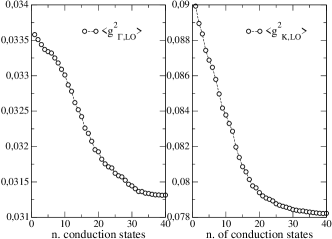
Figure 1: Convergence of the $\mathinner{\langle{g^{2}_{\mathbf{q},\nu}}\rangle}_{F}$ (expressed in eV²) with the number of unoccupied states used to build the two-particle Hamiltonian within the BSE scheme. Values are reported for the symmetry points $\mathbf{q}=\mathbf{\Gamma}$,$\mathbf{K}$ and for the highest optical phonon branch. All calculations have been performed using a 6x6x1 sampling of the BZ

Figure 1 demonstrates that the converged values of $\mathinner{\langle{g^{2}_{\mathbf{\Gamma},\text{LO}}}\rangle}_{F}=0.031$ and $\mathinner{\langle{g^{2}_{\mathbf{K},\text{LO}}}\rangle}_{F}=0.078\,\text{eV}^{2}$, computed within a QS$G\widehat{W}$ scheme, are in excellent agreement with the values obtained at $\mathbf{\Gamma}$ by interpolating the phonon dispersion near the Kohn anomaly (0.031 eV²) and at $\mathbf{K}$ (0.080 eV²) using Eq. (213) with $\omega_{\mathbf{K},\text{LO}}$ from Ref. Lazzeri et al., 2008, respectively. Notably, these values satisfy the condition $\lambda=2.05$. The fulfillment of this condition indicates that our approach did not encompass e-ph vertex corrections in the evaluation of the inverse dielectric function, which indeed was the case. A field-theoretic framework incorporating the static e-ph contribution ($W_{ph}^{\text{A}}$) to the screened Coulomb interaction into the kernel of the two-particle Hamiltonian would enable the introduction of an infinite sum of e-ph vertex diagrams in the BSE-corrected inverse dielectric matrix and account for exciton-phonon coupling. A similar framework should theoretically recover the result $\lambda=5.19$ reported in Ref. Basko and Aleiner, 2008. However, this approach is not pursued in our work, leaving it as a potential area for future exploration. Lastly, it is noteworthy that all the other Fermi surface-average matrix elements $\mathinner{\langle{g^{2}_{\mathbf{q},\nu}}\rangle}_{F}$ at $\mathbf{q}=\mathbf{\Gamma}$,$\mathbf{K}$ and for phonon modes distinct from the highest optical mode are zero, except for the doubly degenerate phonon mode at $\mathbf{K}$. For this mode, QS$GW$ yields $\mathinner{\langle{g^{2}_{\mathbf{K},\nu}}\rangle}_{F}=0.00478\,\text{eV}^{2}$, while QS$G\widehat{W}$ results in $\mathinner{\langle{g^{2}_{\mathbf{K},\nu}}\rangle}_{F}=0.00336\text{eV}^{2}$. This observation is consistent with the conclusions drawn in Ref. Piscanec et al., 2004 as well as with the absence of Kohn anomalies for all these branches.

Conclusions

In this work, we outline a derivation of the electron-phonon matrix element $g_{in,\nu}(\mathbf{k},\mathbf{q})$ and the dynamical matrix within a field theoretic framework, following the seminal works of BaymBaym (1961) and Hedin and LundqvistHedin and Lundqvist (1969). The central quantity is the static electronic dielectric function $\varepsilon_{e}(\mathbf{r},\mathbf{r}^{\prime};0)$, eliminating the need to obtain the the induced density from a Sternheimer equation. Notably, we show that, when suitably formulated, no Pulay-like correction terms are needed to compute the e-ph matrix elements. We also provide detailed insights into how this formalism is implemented within QGSW method and a mixed product basis set formalism in the Questaal package. Furthermore, within the MBPT framework, we illustrate the separation of the e-ph matrix elements into a long-ranged, nonanalytic part and an analytic short-range remainder, providing also an expression for the Born effective charge tensor from first principles. The long-range e-ph term can be regarded as an extension of Fröhlich’s model to anisotropic lattices and multiple phonon modes. Additionally, we demonstrate that the e-ph matrix elements within the LMTO-MPB formalism can be expressed as a linear combination of projection coefficients for the product of two wave functions, simplifying the algorithm for the transformation rule $g_{in,\nu}(\mathbf{k},\mathbf{S}\mathbf{q})$ for rotation of a phonon wave vector.

With Questaal’s ability to compute the polarizability with ladder diagrams, we extended beyond the RPA in computing the inverse dielectric matrix, which mainly contributes to $g_{in,\nu}(\mathbf{k},\mathbf{q})$. Through comprehensive testing of the implemented field-theoretic framework, we demonstrate its ability to yield results in excellent agreement with experimentally derived Fermi surface-averaged electron-phonon matrix elements extracted from the slope of the Kohn anomalies for the highest optical phonon mode in graphene and when electron to multiphonons coupling is neglected.