A Mean Field Game Model for Timely Computation in Edge Computing Systems

Abstract

We consider the problem of task offloading in multi-access edge computing (MEC) systems constituting $N$ devices assisted by an edge server (ES), where the devices can split task execution between a local processor and the ES. Since the local task execution and communication with the ES both consume power, each device must judiciously choose between the two. We model the problem as a large population non-cooperative game among the $N$ devices. Since computation of an equilibrium in this scenario is difficult due to the presence of a large number of devices, we employ the mean-field game framework to reduce the finite-agent game problem to a generic user’s multi-objective optimization problem, with a coupled consistency condition. By leveraging the novel age of information (AoI) metric, we invoke techniques from stochastic hybrid systems (SHS) theory and study the tradeoffs between increasing information freshness and reducing power consumption. In numerical simulations, we validate that a higher load at the ES may lead devices to upload their task to the ES less often.

I Introduction

The multi-access edge computing (MEC) technology has recently attracted wide attention as a promising solution to improve computing capabilities, especially in the resource-limited internet-of-things (IoT) devices [1]. The MEC architecture leverages advances in wireless communication and mobile computing paradigms to allow for offloading task execution to the edge of the network. Edge computing is anticipated to play a crucial role in time-critical applications such as vehicle positioning in autonomous driving, task assignment problems in warehouses, and remote surgery systems [2, 3].

In this work, we aim to: 1) accelerate task execution in MEC-based applications (hence, improve their situational awareness) by employing the novel age of information (AoI) metric [4], and 2) provide a low-complexity decentralized computation offloading algorithm for the IoT devices. Precisely, we model the computation offloading problem in MEC systems comprising $N$ devices and an edge server (ES) using the framework of non-cooperative game theory. An example of such a MEC system is shown in Fig. 1, where in various applications (such as medical, vehicular and home surveillance examples as shown in the figure) devices offload a part of their computation to an ES. To entail tractable equilibrium policy computations, we employ the paradigm of mean-field games (MFGs) [5, 6, 7, 8, 9, 10, 11], to compute approximate Nash equilibrium policies which ensure optimal division of task processing between local processor and the ES.

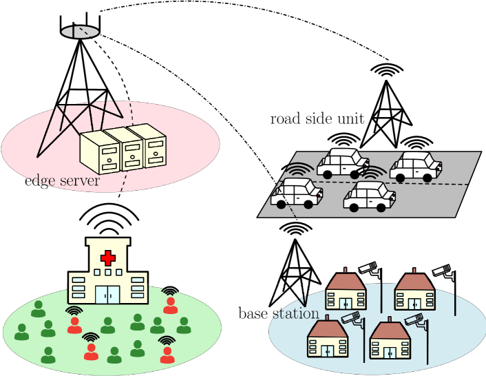
Figure 1: A MEC system model consisting of an edge server (ES) and various applications (medical, vehicular and home surveillance examples are shown in the figure) that utilize the ES for timely computation simultaneously.

Related Work: The subject of computation offloading in MEC systems has been extensively studied over the past decade. Earlier works have focused on minimizing energy consumption, studying power-delay tradeoffs and server-device load balancing problems [12, 13, 14, 1] through the lens of resource allocation when multiple users are involved. The latter problem is then solved using the Lyapunov optimization technique [15, 16] to provide feasible solutions. While timeliness considerations do not appear in the above works, there have been some recent works which focus on timeliness within the realm of MEC resource allocation [17, 18, 3]. Particularly, the paper [17] considers a single-source single-destination MEC system for timely status updating. The authors in [18] leverage energy harvesting in addition to MEC to support computing capabilities of the IoT devices. In [3], the authors jointly assess the impact of stochastic arrivals, scheduling policy, and unreliable channel conditions on the expected sum AoI in MEC assisted IoT networks.

The contribution and distinctiveness of our work are outlined as follows. In contrast to previous studies, we approach the computation offloading problem from a non-cooperative game perspective rather than framing it as a resource allocation problem. The game theoretical aspect then appropriately takes into account the selfish interests of the end-users. Further, the decentralized nature of the game theoretical approach allows for designing low-dimensional optimization problems for the end-users compared to a centralized one. We structure the problem as a power-AoI tradeoff multi-objective optimization problem for each end-user, thereby explicitly addressing the timeliness considerations. First, we derive approximate expressions for the AoI for a system of servers connected both serially and in parallel for sufficiently large arrival rates, where (as we will see later) we cannot employ a fake update approach as proposed in [19]. Then, we obtain a closed-form expression for the AoI for a large number of devices using the MFG setting, thereby formulating the optimality and consistency conditions. Finally, using numerical simulations, we observe that a higher loading at the ES causes devices to offload lesser tasks and vice-versa.

Notations: $[N]:=\{1,\ldots,N\}$ denotes the set of agents. We use the shorthand $\text{exp}(\lambda)$ to denote an exponential random variable with rate $\lambda$. For a policy vector $a=[a_{1},\cdots,a_{N}]$, $a_{-i}$ denotes the policy vector of all users other than user $i$.

II $N$-User Game Problem

We formulate the MEC problem as a multi-user game. Consider the system in Fig. 1 comprising $N$ devices which need to execute their respective incoming tasks. Each device is of a particular type $\phi$ chosen from a finite type set $\Phi$ sampled from a probability distribution $\mathbb{P}_{N}(\phi)$, which appropriately accounts for the heterogeneity among the devices. To assist the devices with task execution, an ES is available. Thus, each device has two options for executing each incoming task: It can either serve it directly using its local processor or it can offload it to the ES using its device transmitter. A schematic diagram of task flow from the perspective of device $i$ is shown in Fig. 2. The inter-arrival times of tasks arriving at the $i$th device $D_{i}$ are distributed as a random variable $\text{exp}(\lambda_{i})$ for all $i\in[N]$. If device $i$ decides to carry out the tasks on the local processor $L_{i}$, then it can operate the processor at a frequency $f_{i}\leq f_{i,max}$. The service time of $L_{i}$ is distributed as an $\text{exp}(f_{i})$ random variable. Accordingly, the processing power usage is given as $P_{\ell,i}=\eta f_{i}^{3}$, where $\eta$ is a positive constant denoting the processor’s effective capacitance [12]. $\eta$ could be chosen user dependent, however, for ease of analysis, we take it to be the same for all devices.

On the other hand, if a device decides to offload the task to the ES, then it gets served sequentially by the device transmitter $T_{i}$ to the ES and the ES uploads it back to the device after processing (as in Fig. 2). The transmission rate of $T_{i}$ is modeled as an $\text{exp}(P_{T,i})$ random variable with rate $P_{T,i}$ being the mean transmission power usage and $P_{T,i}\leq P_{i,max}$. The service rate for the transmitted task at the ES is modeled as an $\text{exp}(\mu_{3}^{(N)})$ random variable where the superscript on $\mu_{3}^{(N)}$ (which is $\gg f_{i},P_{T,i}$) denotes its dependence on the number of devices in the population. The interference from the other devices in the $i$th device’s task flow is denoted (in Fig. 2) by the adder preceding the ES, which receives packets according to an exogeneous process with a combined rate of $\lambda^{(N)}_{e}$. The ES serves tasks using the last-come-first-serve with preemption (LCFS-P) discipline, and the downloading time of the processed task by the device is negligible.

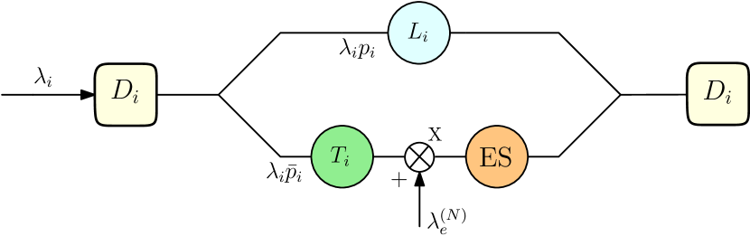
Figure 2: Task flow for device $i$: $D_{i}$, $L_{i}$, $T_{i}$ denote the $i$th device itself, its local processor, and its transmitter, respectively.

Since the effective service rates provided by $L_{i}$ and the series path of $T_{i}$ and the ES are heterogeneous, we employ the i.i.d. Bernoulli distributed random variable with a mean $p_{i}$ to split the incoming Poisson process into two independent Poisson processes with respective means $\lambda_{i}p_{i}$ and $\lambda_{i}\bar{p}_{i}$ where $\bar{p}_{i}=1-p_{i}$ (as in Fig. 2). We note here that traditionally, queue length has been used to measure execution delay [12], which does not take into account the time criticality of the associated tasks. Since time responsiveness is one of the major concerns of this work, we employ the AoI metric which has been widely used to maintain timely updates of the tasks [4].

The objective of each device is two-fold: (1) To minimize the expected AoI of the tasks, and (2) to minimize the power usage during local processing and transmission. Since this is a multi-objective optimization problem, in the sequel we use the scalarization approach [20] to setup each device’s problem.

We are now ready to formally state the optimization problem of the $i$th device. To maintain notational consistency of the service rates, let us use the notation $\mu_{1i}$ to denote $P_{T,i}$, and $\mu_{2i}$ to denote $f_{i}$. Following this, let us define $\bm{\mu}_{1}:=[\mu_{11},\cdots,\mu_{1N}]$, $\bm{\mu}_{2}:=[\mu_{21},\cdots,\mu_{2N}]$ and $\bm{p}:=[p_{1},\cdots,p_{N}]$. Then, each device $i\in[N]$ wishes to solve the following problem.

Problem 1 ($N$-agent game problem)

Each device $i\in[N]$ aims to minimize its cost $J_{N,i}$, given policies of other devices:

$$\min_{p_{i},\mu_{1i},\mu_{2i}} J^{(N)}_{i}(\bm{p},\bm{\mu}_{1},\bm{\mu}_{2}):=\mu_{1i}+\eta\mu_{2i}^{3}+V\Delta^{(N)}_{i}\!(\bm{p},\bm{\mu}_{1},\bm{\mu}_{2})$$

s.t. $$\mu_{1i}\leq P_{i,max}$$

$$\mu_{2i}\leq f_{i,max}$$ (1)

where $V>0$ is the importance weight given for freshness.

We also refer to the triple $(p_{i},\mu_{1i},\mu_{2i})$ as the policy of device $i$. The problem in (1) is a game problem due to the presence of other devices’ policies in the cost optimization problem of the $i$th device. To completely define the above problem, we need to characterize the expression for the average AoI, $\Delta^{(N)}_{i}(\bm{p},\bm{\mu}_{1},\bm{\mu}_{2})$, which we will derive in the next section.

III Age of Information Calculation

We calculate the AoI of the $i$th device using the SHS technique which utilizes tools from control theory and dynamical systems [21, 22, 19] to handle systems involving both discrete and continuous states. For completeness, we briefly review the main concepts of the SHS method.

III-A Stochastic Hybrid Systems (SHS)

The SHS method constitutes a state pair $(s(t),x(t))\in S\times\mathbb{R}^{n+1}$ for all time $t\geq 0$, with $S$ being a finite set. The continuous state $x(t)$ evolves according to a stochastic differential equation $dx(t)=e(t,s,x)dt+g(t,s,x)dB(t)$, where $B(t)$ is a standard Brownian motion. Further, the discrete state $s(t)$ evolves according to a Markov chain from a state $s$ to a state $s^{\prime}$ with transition intensity $q\delta_{s,s^{\prime}}$, and at each transition, the jump in the continuous state is given as $x^{\prime}=h(t,s,x)$. With the above description, AoI can be characterized as a special case of the SHS framework. AoI is defined as the time elapsed at the receiving end since the latest delivered information packet was generated at the source, and serves to quantify the freshness of information at the receiver. A prototypical sample path of the AoI evolution is shown in Fig. 3, which is a piecewise linear SHS with $e(t,s,x)=u_{s},$ $g(t,s,x)=0,$ $u_{s}\in\{0,1\}$, and $h(t,s,x)=xA_{s}$, where $A_{s}\in\{0,1\}^{n+1\times n+1}$.

Following [19], we now define $\pi_{s^{\prime}}(t):=\mathbb{P}(s(t)=s^{\prime})$ as the probability of state $s(t)=s^{\prime}$, and $v_{s^{\prime}_{k}}(t):=\mathbb{P}(x_{k}(t)\mid s(t)=s^{\prime})$ as the conditional probability of the process $x(t)$ given $s(t)=s^{\prime}$. Further, let us denote the set of possible outgoing transitions from a particular state $s$ as $L_{s}:=\{\ell:s_{\ell}=s\}$ and the set of possible incoming transitions to a state $s^{\prime}$ as $L^{\prime}_{s^{\prime}}:=\{\ell:s_{\ell}=s^{\prime}\}$. Then, assuming that the finite state Markov chain (FS-MC) is ergodic, it has a unique steady state distribution $\bar{\pi}:=[\bar{\pi}_{1},\cdots,\bar{\pi}_{m}]$, which satisfies the conservation law,

$$\bar{\pi}_{s}\sum_{\ell\in L_{s}}q^{\ell} =\sum_{\ell^{\prime}\in L^{\prime}_{s}}q^{\ell^{\prime}}\bar{\pi}_{s_{\ell^{\prime}}},\quad\forall s\in S,$$ (2a)

$$\sum_{s\in S}\bar{\pi}_{s} =1,$$ (2b)

where $m:=|S|$. Consequently, we have the following result.

Theorem 1

​[19, Thm. 4] Suppose $\bar{\pi}$ is the state distribution of the FS-MC and there exists a stationary solution $\bar{v}:=[\bar{v}_{1},\cdots,\bar{v}_{m}]$ of the conditional distribution $v_{(\cdot)}(t)$ satisfying,

$$\bar{v}_{s}\sum_{\ell\in L_{s}}q^{\ell}=u_{s}\bar{\pi}_{s}+\sum_{\ell^{\prime}\in L^{\prime}_{s}}q^{\ell^{\prime}}\bar{v}_{s_{\ell^{\prime}}}A_{\ell^{\prime}}.$$ (3)

Then, the average AoI is given by $\Delta:=\sum_{s\in S}\bar{v}_{s0}$.

Next, we will use the above result to compute an approximate expression for ${\Delta}^{(N)}_{i}(\bm{p},\bm{\mu}_{1},\bm{\mu}_{2})$ in the next subsection.

III-B Average AoI for the $i$th Device

Before proceeding, we first observe from Fig. 2 that the other devices’ interference at the point marked as $X$ in between $T_{i}$ and ES may not obey a Poisson distribution, which makes it challenging to compute the exact expression for ${\Delta}^{(N)}_{i}(\bm{p},\bm{\mu}_{1},\bm{\mu}_{2})$. Additionally, the same prevents us from utilizing the fake update approach for all servers as proposed in [19], which is commonly employed to reduce the dimension of the state space. Thus, to facilitate a tractable analysis, we take $\lambda_{i}$’s to be large, which then entails that the aforementioned distribution can be closely approximated by a $\text{exp}(\lambda_{e}^{(N)})$ distribution [19], where we define $\lambda_{e}^{(N)}:=\sum_{j=1,j\neq i}^{N}\frac{\lambda_{j}\bar{p}_{j}\mu_{1j}}{\lambda_{j}\bar{p}_{j}+\mu_{1j}}$.

Figure 3: Evolution of the AoI at the receiver.

Next, we formulate the state space and transition functions of the FS-MC. In this regard, let us define $\rho^{(N)}:=\frac{\lambda_{e}^{(N)}}{\mu^{(N)}_{3}}$. Also, henceforth, we refer to device $i$’s own packets as packets of class 1 and the exogenous packets as those of class 2.

The state space $S$ comprises 8 states which keep track of the server holding the freshest and second freshest packets, and the oldest packet of class 1, and the server holding a packet of class 2. Detailed descriptions are provided in Table I.

state	server 1 ($T_{i}$)	server 2 $(L_{i})$	server 3 (ES)
$s_{1}$	freshest	$2^{nd}$ freshest	oldest
$s_{2}$	freshest	oldest	$2^{nd}$ freshest
$s_{3}$	$2^{nd}$ freshest	freshest	oldest
$s_{4}$	no packet	freshest	$2^{nd}$ freshest
$s_{5}$	no packet	$2^{nd}$freshest	freshest
$s_{6}$	no packet	freshest	class 2
$s_{7}$	freshest	$2^{nd}$ freshest	class 2
$s_{8}$	$2^{nd}$ freshest	freshest	class 2

TABLE I: State dictionary for the finite FS-MC.

Next, in Table II, we list the possible transitions in the FS-MC and the corresponding AoI vector $x^{\prime}(t):=[x^{\prime}_{0}(t)~{}x^{\prime}_{1}(t)~{}x^{\prime}_{2}(t)~{}x^{\prime}_{3}(t)]$, where $x^{\prime}_{0}(t),$ $x^{\prime}_{1}(t),$ $x^{\prime}_{2}(t)$, and $x^{\prime}_{3}(t)$ denote the AoI at the $i$th device, the local processor, the transmitter, and the ES, respectively, after transition to $s^{\prime}$. Note that henceforth we forego the subscript index $i$ for brevity.

$s$	$q$	$s^{\prime}$	$x^{\prime}=xA_{s}$	$v_{s}A_{s}$
$s_{1}$	$\lambda p$	$s_{3}$	$[x_{0}~{}x_{1}~{}0~{}x_{3}]$	$[\bar{v}_{10}~{}\bar{v}_{11}~{}0~{}\bar{v}_{13}]$
	$\lambda\bar{p}$	$s_{1}$	$[x_{0}~{}0~{}x_{2}~{}x_{3}]$	$[\bar{v}_{10}~{}0~{}\bar{v}_{12}~{}\bar{v}_{13}]$
	$\lambda_{e}^{(N)}$	$s_{7}$	$[x_{0}~{}x_{1}~{}x_{2}~{}x_{0}]$	$[\bar{v}_{10}~{}\bar{v}_{11}~{}\bar{v}_{12}~{}\bar{v}_{10}]$
	$\mu_{1}$	$s_{5}$	$[x_{0}~{}0~{}x_{2}~{}x_{1}]$	$[\bar{v}_{10}~{}0~{}\bar{v}_{12}~{}\bar{v}_{11}]$
	$\mu_{2}$	$s_{1}$	$[x_{2}~{}x_{1}~{}x_{2}~{}x_{2}]$	$[\bar{v}_{12}~{}\bar{v}_{11}~{}\bar{v}_{12}~{}\bar{v}_{12}]$
	$\mu_{3}^{(N)}$	$s_{1}$	$[x_{3}~{}x_{1}~{}x_{2}~{}x_{3}]$	$[\bar{v}_{13}~{}\bar{v}_{11}~{}\bar{v}_{12}~{}\bar{v}_{13}]$
$s_{2}$	$\lambda p$	$s_{3}$	$[x_{0}~{}x_{1}~{}0~{}x_{3}]$	$[\bar{v}_{20}~{}\bar{v}_{21}~{}0~{}\bar{v}_{23}]$
	$\lambda\bar{p}$	$s_{2}$	$[x_{0}~{}0~{}x_{2}~{}x_{3}]$	$[\bar{v}_{20}~{}0~{}\bar{v}_{22}~{}\bar{v}_{23}]$
	$\lambda_{e}^{(N)}$	$s_{7}$	$[x_{0}~{}x_{1}~{}x_{2}~{}x_{0}]$	$[\bar{v}_{20}~{}\bar{v}_{21}~{}\bar{v}_{22}~{}\bar{v}_{20}]$
	$\mu_{1}$	$s_{5}$	$[x_{0}~{}0~{}x_{2}~{}x_{1}]$	$[\bar{v}_{20}~{}0~{}\bar{v}_{22}~{}\bar{v}_{21}]$
	$\mu_{2}$	$s_{2}$	$[x_{2}~{}x_{1}~{}x_{2}~{}x_{3}]$	$[\bar{v}_{22}~{}\bar{v}_{21}~{}\bar{v}_{22}~{}\bar{v}_{23}]$
	$\mu_{3}^{(N)}$	$s_{2}$	$[x_{3}~{}x_{1}~{}x_{3}~{}x_{3}]$	$[\bar{v}_{23}~{}\bar{v}_{21}~{}\bar{v}_{23}~{}\bar{v}_{23}]$
$s_{3}$	$\lambda p$	$s_{3}$	$[x_{0}~{}x_{1}~{}0~{}x_{3}]$	$[\bar{v}_{30}~{}\bar{v}_{31}~{}0~{}\bar{v}_{33}]$
	$\lambda\bar{p}$	$s_{1}$	$[x_{0}~{}0~{}x_{2}~{}x_{3}]$	$[\bar{v}_{30}~{}0~{}\bar{v}_{32}~{}\bar{v}_{33}]$
	$\lambda_{e}^{(N)}$	$s_{8}$	$[x_{0}~{}x_{1}~{}x_{2}~{}x_{0}]$	$[\bar{v}_{30}~{}\bar{v}_{31}~{}\bar{v}_{32}~{}\bar{v}_{30}]$
	$\mu_{1}$	$s_{4}$	$[x_{0}~{}0~{}x_{2}~{}x_{1}]$	$[\bar{v}_{30}~{}0~{}\bar{v}_{32}~{}\bar{v}_{31}]$
	$\mu_{2}$	$s_{3}$	$[x_{2}~{}x_{2}~{}x_{2}~{}x_{2}]$	$[\bar{v}_{32}~{}\bar{v}_{32}~{}\bar{v}_{32}~{}\bar{v}_{32}]$
	$\mu_{3}^{(N)}$	$s_{3}$	$[x_{3}~{}x_{1}~{}x_{2}~{}x_{3}]$	$[\bar{v}_{33}~{}\bar{v}_{31}~{}\bar{v}_{32}~{}\bar{v}_{33}]$
$s_{4}$	$\lambda p$	$s_{4}$	$[x_{0}~{}0~{}0~{}x_{3}]$	$[\bar{v}_{40}~{}0~{}0~{}\bar{v}_{43}]$
	$\lambda\bar{p}$	$s_{1}$	$[x_{0}~{}0~{}x_{2}~{}x_{3}]$	$[\bar{v}_{40}~{}0~{}\bar{v}_{42}~{}\bar{v}_{43}]$
	$\lambda_{e}^{(N)}$	$s_{6}$	$[x_{0}~{}0~{}x_{2}~{}x_{0}]$	$[\bar{v}_{40}~{}0~{}\bar{v}_{42}~{}\bar{v}_{40}]$
	$\mu_{2}$	$s_{4}$	$[x_{2}~{}0~{}x_{2}~{}x_{2}]$	$[\bar{v}_{42}~{}0~{}\bar{v}_{42}~{}\bar{v}_{42}]$
	$\mu_{3}^{(N)}$	$s_{4}$	$[x_{3}~{}0~{}x_{2}~{}x_{3}]$	$[\bar{v}_{43}~{}0~{}\bar{v}_{42}~{}\bar{v}_{43}]$
$s_{5}$	$\lambda p$	$s_{4}$	$[x_{0}~{}0~{}0~{}x_{3}]$	$[\bar{v}_{50}~{}0~{}0~{}\bar{v}_{53}]$
	$\lambda\bar{p}$	$s_{2}$	$[x_{0}~{}0~{}x_{2}~{}x_{3}]$	$[\bar{v}_{50}~{}0~{}\bar{v}_{52}~{}\bar{v}_{53}]$
	$\lambda_{e}^{(N)}$	$s_{6}$	$[x_{0}~{}0~{}x_{2}~{}x_{0}]$	$[\bar{v}_{50}~{}0~{}\bar{v}_{52}~{}\bar{v}_{50}]$
	$\mu_{2}$	$s_{5}$	$[x_{2}~{}0~{}x_{2}~{}x_{3}]$	$[\bar{v}_{52}~{}0~{}\bar{v}_{52}~{}\bar{v}_{53}]$
	$\mu_{3}^{(N)}$	$s_{5}$	$[x_{3}~{}0~{}x_{3}~{}x_{3}]$	$[\bar{v}_{53}~{}0~{}\bar{v}_{53}~{}\bar{v}_{53}]$
$s_{6}$	$\lambda p$	$s_{6}$	$[x_{0}~{}0~{}0~{}x_{3}]$	$[\bar{v}_{60}~{}0~{}0~{}\bar{v}_{63}]$
	$\lambda\bar{p}$	$s_{7}$	$[x_{0}~{}0~{}x_{2}~{}x_{3}]$	$[\bar{v}_{60}~{}0~{}\bar{v}_{62}~{}\bar{v}_{63}]$
	$\lambda_{e}^{(N)}$	$s_{6}$	$[x_{0}~{}0~{}x_{2}~{}x_{0}]$	$[\bar{v}_{60}~{}0~{}\bar{v}_{62}~{}\bar{v}_{60}]$
	$\mu_{2}$	$s_{6}$	$[x_{2}~{}0~{}x_{2}~{}x_{2}]$	$[\bar{v}_{62}~{}0~{}\bar{v}_{62}~{}\bar{v}_{62}]$
	$\mu_{3}^{(N)}$	$s_{6}$	$[x_{3}~{}0~{}x_{2}~{}x_{3}]$	$[\bar{v}_{63}~{}0~{}\bar{v}_{62}~{}\bar{v}_{63}]$
$s_{7}$	$\lambda p$	$s_{8}$	$[x_{0}~{}x_{1}~{}0~{}x_{3}]$	$[\bar{v}_{70}~{}\bar{v}_{71}~{}0~{}\bar{v}_{73}]$
	$\lambda\bar{p}$	$s_{7}$	$[x_{0}~{}0~{}x_{2}~{}x_{3}]$	$[\bar{v}_{70}~{}0~{}\bar{v}_{72}~{}\bar{v}_{73}]$
	$\lambda_{e}^{(N)}$	$s_{7}$	$[x_{0}~{}x_{1}~{}x_{2}~{}x_{0}]$	$[\bar{v}_{70}~{}\bar{v}_{71}~{}\bar{v}_{72}~{}\bar{v}_{70}]$
	$\mu_{1}$	$s_{5}$	$[x_{0}~{}0~{}x_{2}~{}x_{1}]$	$[\bar{v}_{70}~{}0~{}\bar{v}_{72}~{}\bar{v}_{71}]$
	$\mu_{2}$	$s_{7}$	$[x_{2}~{}x_{1}~{}x_{2}~{}x_{2}]$	$[\bar{v}_{72}~{}\bar{v}_{71}~{}\bar{v}_{72}~{}\bar{v}_{72}]$
	$\mu_{3}^{(N)}$	$s_{7}$	$[x_{3}~{}x_{1}~{}x_{2}~{}x_{3}]$	$[\bar{v}_{73}~{}\bar{v}_{71}~{}\bar{v}_{72}~{}\bar{v}_{73}]$
$s_{8}$	$\lambda p$	$s_{8}$	$[x_{0}~{}x_{1}~{}0~{}x_{3}]$	$[\bar{v}_{80}~{}\bar{v}_{81}~{}0~{}\bar{v}_{83}]$
	$\lambda\bar{p}$	$s_{7}$	$[x_{0}~{}0~{}x_{2}~{}x_{3}]$	$[\bar{v}_{80}~{}0~{}\bar{v}_{82}~{}\bar{v}_{83}]$
	$\lambda_{e}^{(N)}$	$s_{8}$	$[x_{0}~{}x_{1}~{}x_{2}~{}x_{0}]$	$[\bar{v}_{80}~{}\bar{v}_{81}~{}\bar{v}_{82}~{}\bar{v}_{80}]$
	$\mu_{1}$	$s_{4}$	$[x_{0}~{}0~{}x_{2}~{}x_{1}]$	$[\bar{v}_{80}~{}0~{}\bar{v}_{82}~{}\bar{v}_{81}]$
	$\mu_{2}$	$s_{8}$	$[x_{2}~{}x_{2}~{}x_{2}~{}x_{2}]$	$[\bar{v}_{82}~{}\bar{v}_{82}~{}\bar{v}_{82}~{}\bar{v}_{82}]$
	$\mu_{3}^{(N)}$	$s_{8}$	$[x_{3}~{}x_{1}~{}x_{2}~{}x_{3}]$	$[\bar{v}_{83}~{}\bar{v}_{81}~{}\bar{v}_{82}~{}\bar{v}_{83}]$

TABLE II: State transitions of the FS-MC and associated AoI jumps

Finally, we assume that all servers which do not precede a node of packet arrival are busy all the time, i.e., whenever a packet leaves a server, a fake packet with the same type and AoI as the departing one starts processing. It is essential to take care of the emphasized statement, since in our case server 1 precedes the point of arrival of exogeneous packets. Thus, the SHS model should take into account whether it is idling or is busy, and hence, we cannot run a fake update at this server. Consequently, we have that $u_{s}=[1~{}1~{}1~{}1]$ for $s=s_{1},s_{2},s_{3},s_{7},s_{8},$ and $u_{s}:=\hat{u}_{s}=[1~{}0~{}1~{}1]$ for $s=s_{4},s_{5},s_{6}$.

Let us define $a:=\lambda+\lambda_{e}^{(N)}+\mu_{1}+\mu_{2}+\mu_{3}^{(N)}$ and $\hat{a}:=a-\mu_{1}$. Then, using (2), $\bar{\pi}$ satisfies (2b) and the following equations,

$$a\bar{\pi}_{1} =(\lambda\bar{p}+\mu_{2}+\mu_{3}^{(N)})\bar{\pi}_{1}+\lambda\bar{p}(\bar{\pi}_{3}+\bar{\pi}_{4}),$$ (4a)

$$a\bar{\pi}_{2} =(\lambda\bar{p}+\mu_{2}+\mu_{3}^{(N)})\bar{\pi}_{2}+\lambda\bar{p}\bar{\pi}_{5},$$ (4b)

$$a\bar{\pi}_{3} =(\lambda p+\mu_{2}+\mu_{3}^{(N)})\bar{\pi}_{3}+\lambda p(\bar{\pi}_{1}+\bar{\pi}_{2}),$$ (4c)

$$\hat{a}\bar{\pi}_{4} =(\lambda p+\mu_{2}+\mu_{3}^{(N)})\bar{\pi}_{4}\!+\!\lambda p\bar{\pi}_{5}\!+\!\mu_{1}(\bar{\pi}_{3}\!+\!\bar{\pi}_{8}),\!\!$$ (4d)

$$\hat{a}\bar{\pi}_{5} =(\mu_{2}+\mu_{3}^{(N)})\bar{\pi}_{5}+\mu_{1}(\bar{\pi}_{1}+\bar{\pi}_{2}+\bar{\pi}_{7}),$$ (4e)

$$\hat{a}\bar{\pi}_{6} =(\lambda p+\lambda_{e}^{(N)}+\mu_{2}+\mu_{3}^{(N)})\bar{\pi}_{6}+\lambda_{e}^{(N)}(\bar{\pi}_{4}+\bar{\pi}_{5}),$$ (4f)

$$a\bar{\pi}_{7} =(\lambda\bar{p}+\lambda_{e}^{(N)}+\mu_{2}+\mu_{3}^{(N)})\bar{\pi}_{7}+\lambda_{e}^{(N)}(\bar{\pi}_{1}+\bar{\pi}_{2})$$

$$~{}~{}~{}+\!\lambda\bar{p}(\bar{\pi}_{6}+\bar{\pi}_{8}),$$ (4g)

$$a\bar{\pi}_{8} =(\lambda p\!+\!\lambda_{e}^{(N)}\!\!+\!\mu_{2}\!+\!\mu_{3}^{(N)}\!)\bar{\pi}_{8}\!+\!\lambda_{e}^{(N)}\!(\bar{\pi}_{3})\!+\!\lambda p\bar{\pi}_{7}.\!\!$$ (4h)

$$a\bar{v}_{1} \!=\!u_{s}\bar{\pi}_{1}\!+\!\lambda\bar{p}[\bar{v}_{10}~{}0~{}\bar{v}_{12}~{}\bar{v}_{13}]+\mu_{2}[\bar{v}_{12}~{}\bar{v}_{11}~{}\bar{v}_{12}~{}\bar{v}_{12}]+\mu_{3}^{(N)}[\bar{v}_{13}~{}\bar{v}_{11}~{}\bar{v}_{12}~{}\bar{v}_{13}]+\lambda\bar{p}[\bar{v}_{30}~{}0~{}\bar{v}_{32}~{}\bar{v}_{33}]+\lambda\bar{p}[\bar{v}_{40}~{}0~{}\bar{v}_{42}~{}\bar{v}_{43}]$$ (5a)

$$a\bar{v}_{2} =u_{s}\bar{\pi}_{2}+\lambda\bar{p}[\bar{v}_{20}~{}0~{}\bar{v}_{22}~{}\bar{v}_{23}]+\mu_{2}[\bar{v}_{22}~{}\bar{v}_{21}~{}\bar{v}_{22}~{}\bar{v}_{23}]+\mu_{3}^{(N)}[\bar{v}_{23}~{}\bar{v}_{21}~{}\bar{v}_{23}~{}\bar{v}_{23}]+\lambda\bar{p}[\bar{v}_{50}~{}0~{}\bar{v}_{52}~{}\bar{v}_{53}]$$ (5b)

$$a\bar{v}_{3} \!=\!u_{s}\bar{\pi}_{3}+\lambda p[\bar{v}_{30}~{}\bar{v}_{31}~{}0~{}\bar{v}_{33}]\!+\!\mu_{2}[\bar{v}_{32}~{}\bar{v}_{32}~{}\bar{v}_{32}~{}\bar{v}_{32}]+\mu_{3}^{(N)}[\bar{v}_{33}~{}\bar{v}_{31}~{}\bar{v}_{32}~{}\bar{v}_{33}]+\lambda p[\bar{v}_{10}~{}\bar{v}_{11}~{}0~{}\bar{v}_{13}]+\lambda p[\bar{v}_{20}~{}\bar{v}_{21}~{}0~{}\bar{v}_{23}]$$ (5c)

$$\hat{a}\bar{v}_{4} =\hat{u}_{s}\bar{\pi}_{4}+\lambda p[\bar{v}_{40}~{}0~{}0~{}\bar{v}_{43}]+\mu_{2}[\bar{v}_{42}~{}0~{}\bar{v}_{42}~{}\bar{v}_{42}]+\mu_{3}^{(N)}[\bar{v}_{43}~{}0~{}\bar{v}_{42}~{}\bar{v}_{43}]+\lambda p[\bar{v}_{50}~{}0~{}0~{}\bar{v}_{53}]+\mu_{1}[\bar{v}_{30}~{}0~{}\bar{v}_{32}~{}\bar{v}_{31}]$$

$$~{}~{}+\mu_{1}[\bar{v}_{80}~{}0~{}\bar{v}_{82}~{}\bar{v}_{81}]$$ (5d)

$$\hat{a}\bar{v}_{5} =\hat{{u}}_{s}\bar{\pi}_{5}+\mu_{1}[\bar{v}_{70}~{}0~{}\bar{v}_{72}~{}\bar{v}_{71}]+\mu_{2}[\bar{v}_{52}~{}0~{}\bar{v}_{52}~{}\bar{v}_{53}]+\mu_{3}^{(N)}[\bar{v}_{53}~{}0~{}\bar{v}_{53}~{}\bar{v}_{53}]+\mu_{1}[\bar{v}_{10}~{}0~{}\bar{v}_{12}~{}\bar{v}_{11}]+\mu_{1}[\bar{v}_{20}~{}0~{}\bar{v}_{22}~{}\bar{v}_{21}]$$ (5e)

$$\hat{a}\bar{v}_{6} =\hat{{u}}_{s}\bar{\pi}_{6}+\lambda p[\bar{v}_{60}~{}0~{}0~{}\bar{v}_{63}]+\lambda_{e}^{(N)}[\bar{v}_{40}~{}0~{}\bar{v}_{42}~{}\bar{v}_{40}]+\mu_{2}[\bar{v}_{62}~{}0~{}\bar{v}_{62}~{}\bar{v}_{62}]+\mu_{3}^{(N)}[\bar{v}_{63}~{}0~{}\bar{v}_{62}~{}\bar{v}_{63}]+\lambda_{e}^{(N)}[\bar{v}_{50}~{}0~{}\bar{v}_{52}~{}\bar{v}_{50}]$$

$$~{}~{}+\lambda_{e}^{(N)}[\bar{v}_{60}~{}0~{}\bar{v}_{62}~{}\bar{v}_{60}]$$ (5f)

$$a\bar{v}_{7} =u_{s}\bar{\pi}_{7}+\lambda\bar{p}[\bar{v}_{60}~{}0~{}\bar{v}_{62}~{}\bar{v}_{63}]+\lambda\bar{p}[\bar{v}_{70}~{}0~{}\bar{v}_{72}~{}\bar{v}_{73}]+\lambda\bar{p}[\bar{v}_{80}~{}0~{}\bar{v}_{82}~{}\bar{v}_{83}]+\lambda_{e}^{(N)}[\bar{v}_{10}~{}\bar{v}_{11}~{}\bar{v}_{12}~{}\bar{v}_{10}]+\lambda_{e}^{(N)}[\bar{v}_{20}~{}\bar{v}_{21}~{}\bar{v}_{22}~{}\bar{v}_{20}]$$

$$~{}~{}+\lambda_{e}^{(N)}[\bar{v}_{70}~{}\bar{v}_{71}~{}\bar{v}_{72}~{}\bar{v}_{70}]+\mu_{3}^{(N)}[\bar{v}_{73}~{}\bar{v}_{71}~{}\bar{v}_{72}~{}\bar{v}_{73}]+\mu_{2}[\bar{v}_{72}~{}\bar{v}_{71}~{}\bar{v}_{72}~{}\bar{v}_{72}]$$ (5g)

$$a\bar{v}_{8} =u_{s}\bar{\pi}_{8}+\lambda p[\bar{v}_{70}~{}\bar{v}_{71}~{}0~{}\bar{v}_{73}]+\lambda_{e}^{(N)}[\bar{v}_{30}~{}\bar{v}_{31}~{}\bar{v}_{32}~{}\bar{v}_{30}]+\lambda_{e}^{(N)}[\bar{v}_{80}~{}\bar{v}_{81}~{}\bar{v}_{82}~{}\bar{v}_{80}]+\mu_{2}[\bar{v}_{82}~{}\bar{v}_{82}~{}\bar{v}_{82}~{}\bar{v}_{82}]$$

$$~{}~{}+\mu_{3}^{(N)}[\bar{v}_{83}~{}\bar{v}_{81}~{}\bar{v}_{82}~{}\bar{v}_{83}]+\lambda p[\bar{v}_{80}~{}\bar{v}_{81}~{}0~{}\bar{v}_{83}]$$ (5h)

 

Then, using (3), the steady-state conditional distribution vector satisfies the set of equations given in (5). We resume the use of subscript $i$ notation and state the main result.

Theorem 2

Suppose the inter-arrivals at device $i$ are distributed as $\text{exp}(\lambda_{i})$ and the service rates as $\text{exp}(\mu_{1i})$ and $\text{exp}(\mu_{2i})$. Let the service rate of the ES be distributed as $\text{exp}(\mu_{3}^{(N)})$. Then, the average AoI ${\Delta}^{(N)}_{i}(\bm{p},\bm{\mu}_{1},\bm{\mu}_{2})$ exists and is given by solving (2) and (5). $\blacksquare$

The proof of the above theorem follows by explicitly solving the set of linear equations (2) to get $\bar{\pi}_{i}$, substituting them in (5) and solving the latter set of equations. The existence is guaranteed by Theorem 1.

$${\Delta}_{\phi}(p_{\phi},\mu_{1\phi},\mu_{2\phi},\rho) =\frac{(1+\rho)}{\lambda_{1\phi}}\frac{\lambda_{1\phi}^{3}m_{1\phi}+\lambda_{1\phi}^{2}m_{2\phi}+\lambda_{1\phi}m_{3\phi}+\mu_{1\phi}\mu_{2\phi}(\mu_{1\phi}+\mu_{2\phi})(1+\rho)}{(\mu_{1\phi}+\lambda_{1\phi}p_{\phi}(1+\rho)+\mu_{1\phi}p_{\phi}\rho)(\mu_{2\phi}(\mu_{1\phi}+\mu_{2\phi})(1+\rho)+\lambda_{1\phi}\bar{p}_{\phi}(\mu_{1\phi}+\mu_{2\phi}(1+\rho))}$$ (6a)

$$m_{1\phi}:=(1+\rho)p_{\phi}\bar{p}_{\phi}$$ (6b)

$$m_{2\phi}:=\mu_{2\phi}(1+\rho)+\mu_{1\phi}(1+(2-p_{\phi})p_{\phi}\rho)$$ (6c)

$$m_{3\phi}:=(1+\rho)(\mu_{1\phi}+\mu_{2\phi})^{2}-\mu_{1\phi}^{2}\bar{p}_{\phi}\rho$$ (6d)

 

Remark 1

We note here that in the literature the offloading problem has been mostly approached using the framework of constrained optimal control rather than a game [12, 18]. In this work, however, we model the problem using a non-cooperative game to account for the effect of other devices’ policies on each device. Additionally, an AoI-based cost function helps us leverage its time responsiveness with respect to end-to-end packet delivery. We also note here that the employed static optimization framework is closer in spirit to policy optimization methods [23] in reinforcement learning (RL) which have recently received great attention in a broad community. Thus, our work can be easily extended to the case with unknown ES parameters and packet arrival rates, which we leave as a promising future research direction.

IV Mean-Field Game

With the AoI calculations in the above subsection, we have provided a complete formulation of the $N$-user game problem. A suitable solution concept for the above game is that of Nash equilibrium [24]. However, its computation becomes intractable due to the high population regime. Thus, to alleviate this issue, we design Nash policies with the additional attractive feature that each agent uses only its local information. In this regard, we leverage the framework of MFGs [7]. Under the latter, we consider the limiting case ($N=\infty$) of the finite-agent system (called the MF system). In this scenario, the individual agent’s deviations from equilibrium policies become insignificant due to the presence of infinite number of agents. Hence, it suffices to consider the viewpoint of generic agents (representing the population of a specific type) which play against a mass distribution rather than each individual agent. This then allows for the computation of the MF equilibrium, which constitutes an optimal policy of a generic agent which is consistent with that of the population.

In the next subsection, we set up the generic agent’s optimization problem using the MFG framework.

IV-A Generic Device’s Optimization Problem

In this subsection, we state the optimization problem faced by the generic device in the infinite population regime. The packets arrive at a generic device of type $\phi$ at mean rate $\lambda_{\phi}$. The tasks are split by employing an i.i.d. Bernoulli distributed random variable with a mean $p_{\phi}$ into two independent Poisson processes with respective means $\lambda_{\phi}p_{\phi}$ and $\lambda_{\phi}\bar{p}_{\phi}$. Further, the mean service rates of the generic transmitter and the generic local processor are given as $\mu_{1,\phi}$ and $\mu_{2,\phi}$, respectively.

Let us define the average AoI of the packets of class 1 as ${\Delta}_{\phi}(p_{\phi},\mu_{1\phi},\mu_{2\phi},\rho):=\lim_{N\rightarrow\infty}\Delta^{(N)}_{i}(\bm{p},\bm{\mu}_{1},\bm{\mu}_{2})$ where $\rho:=\lim_{N\rightarrow\infty}\rho^{(N)}$. The latter exists, for instance, when the service rate of the ES increases proportionally to the number of devices, i.e., when $\mu_{3}^{(N)}=N\mu_{3}$, where $\mu_{3}>0$. The term $\rho$ serves as the MF approximation to the coupling term $\rho^{(N)}$ in the finite-device system and can be viewed as the mean load on the ES in the infinite-device system. Then, we have the generic device optimization problem as follows.

Problem 2 (Generic device optimization problem)

$$\min_{(p_{\phi},\mu_{1\phi},\mu_{2\phi})\in[0,1]\times\mathbb{R}^{2}} J_{\rho}(p_{\phi},\mu_{1\phi},\mu_{2\phi})$$

s.t. $$\mu_{1\phi}\leq P_{\phi,max}$$

$$\mu_{2\phi}\leq f_{\phi,max}$$ (7)

where

$$J_{\rho}(p_{\phi},\mu_{1\phi},\mu_{2\phi}) \!:=\!\mu_{1,\phi}+\eta\mu_{2\phi}^{3}\!+\!V{\Delta}_{\phi}(p_{\phi},\mu_{1\phi},\mu_{2\phi},\rho)$$ (8)

and ${\Delta}_{\phi}(p_{\phi},\mu_{1\phi},\mu_{2\phi},\rho)$ is given in (6a).

Consequently, the MFG is defined using the optimality and the consistency conditions as follows:

1. Optimality: $(\hat{p}_{\phi},\hat{\mu}_{1\phi},\hat{\mu}_{2\phi})\!=\!\arg\min J_{\rho}(p_{\phi},\mu_{1\phi},\mu_{2\phi})$,

2. Consistency: $\hat{\rho}=\frac{1}{\mu_{3}}\mathbb{E}_{\phi}\left[\frac{\lambda_{\phi}\hat{\bar{p}}_{\phi}\hat{\mu}_{2\phi}}{\lambda_{\phi}\hat{\bar{p}}_{\phi}+\hat{\mu}_{2\phi}}\right]$.

Briefly, for a given value of $\rho$, the generic agent solves for an optimal policy using the optimality condition. Consequently, it uses the obtained policy to regenerate $\rho$ using the consistency condition. The mean-field equilibrium (MFE), which constitutes the pair $((p_{\phi,\text{MFE}},\mu_{1\phi,\text{MFE}},\mu_{2\phi,\text{MFE}}),\rho_{\text{MFE}})$, is then given by the fixed point of the composite map induced by 1) and 2) for all $\phi\in\Phi$. Detailed fixed point iteration process is given in Algorithm 1 below.

Algorithm 1 Fixed point iteration for a generic device

1:Input: $V,\eta,\mu_{3},\lambda_{\phi},~{}\forall\phi$ # system parameters

2:Input: $\epsilon$ # approximation parameter

3:Input: $\gamma$ # iteration step size

4:Initialize: $\hat{\rho},p_{\phi}^{(0)},\mu_{1\phi}^{(0)},\mu_{2\phi}^{(0)}=0,~{}\forall\phi$

5:while $|\hat{\rho}^{(m)}-\hat{\rho}^{(m-1)}|<\epsilon$ do

6:   $(\hat{p}^{(k)}_{\phi},\hat{\mu}_{1\phi}^{(k)},\hat{\mu}_{2\phi}^{(k)})\leftarrow\text{argmin }J_{\hat{\rho}^{(k-1)}}(p_{\phi}^{(k-1}\!\!,\mu_{1\phi}^{(k-1)}\!\!,\mu_{2\phi}^{(k-1)})$

7:   $\hat{\rho}^{(k)}\leftarrow(1-\gamma)\hat{\rho}^{(k-1)}+\gamma\mathbb{E}_{\phi}\frac{\lambda_{\phi}(1-\hat{p}^{(k)}_{\phi})\hat{\mu}_{2,\phi}^{(k)}}{\mu_{3}(\lambda_{\phi}(1-\hat{p}^{(k)}_{\phi})+\hat{\mu}_{2\phi)}^{(k)}}$

8:end while

9:Output: $\hat{\rho}^{(m)},(\hat{p}^{(m)}_{\phi},\hat{\mu}_{1\phi}^{(m)},\hat{\mu}_{2\phi}^{(m)}),~{}\forall\phi.$

V Numerical Results

Here, we provide a numerical computation of the MFE for a population of a single type. In the first numerical study, in Fig. 4, we observe that as the mean loading at the ES increases (on the $x$-axis), the optimal probability of using the local processor (on the $y$-axis) increases and that of offloading to the ES decreases. This should be expected since if the ES is heavily loaded, the device is better-off serving tasks locally to incur a lower AoI. Next, in Fig. 5, we plot the variation of the MFE as a function of the arrival rate $\lambda$ and service rate $\mu_{3}$. From the figure, we observe that at equilibrium increasing arrival rate offloads more computations, thereby increasing the ES loading. On the other hand, increasing ES service rate increases offloading by the device, but with a decrease in the mean ES loading, thereby suggesting a slower than linear optimal rate of task offloading by the devices.

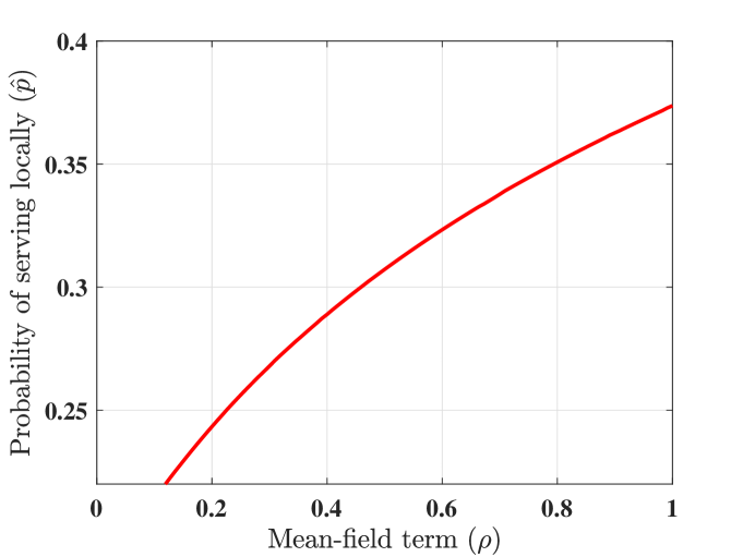
Figure 4: The optimal probability $\hat{p}$ as a function of the MF term $\rho$.

VI Discussion and Conclusion

As a recap, in this work we have considered a timely task computation problem in a MEC system where the devices can either process their tasks on their local processors or offload them to an ES. We have developed a finite-agent Nash game and a MFG model for the task offloading problem in MEC systems, and numerically computed an equilibrium solution to the MF system. In the future, we plan to investigate two important aspects of the above developments: (1) Characterization of the conditions ensuring existence and (possible) uniqueness of the MFE, and (2) a theoretical analysis of the performance of the MFE solution on the original finite-agent system.

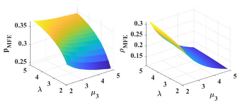
Figure 5: The equilibrium probability $p_{\text{MFE}}$ and equilibrium load $\rho_{\text{MFE}}$ with generic arrival rate $\lambda$ and $\mu_{3}$.

References

• [1] Y. Mao, C. You, J. Zhang, K. Huang, and K. B. Letaief. A survey on mobile edge computing: The communication perspective. IEEE Communications Surveys & Tutorials, 19(4):2322–2358, August 2017.
• [2] M. Hua, Y. Huang, Y. Wang, Q. Wu, H. Dai, and L. Yang. Energy optimization for cellular-connected multi-uav mobile edge computing systems with multi-access schemes. Journal of Communications and Information Networks, 3(4):33–44, December 2018.
• [3] A. Muhammad, I. Sorkhoh, M. Samir, D. Ebrahimi, and C. Assi. Minimizing age of information in multiaccess-edge-computing-assisted IoT networks. IEEE Internet of Things Journal, 9(15):13052–13066, December 2021.
• [4] R. D. Yates, Y. Sun, D. R. Brown, S. K. Kaul, E. Modiano, and S. Ulukus. Age of information: An introduction and survey. IEEE Journal on Sel. Areas in Communication, 39(5):1183–1210, May 2021.
• [5] M. Huang, P. E. Caines, and R. P. Malhamé. Uplink power adjustment in wireless communication systems: A stochastic control analysis. IEEE Transactions on Automatic Control, 49(10):1693–1708, October 2004.
• [6] M. Huang, R. P. Malhamé, and P. E. Caines. Large population stochastic dynamic games: closed-loop Mckean-Vlasov systems and the Nash Certainty Equivalence principle. Communications in Information & Systems, 6(3):221–252, 2006.
• [7] M. Huang, P. E. Caines, and R. P. Malhamé. Large-population cost-coupled LQG problems with nonuniform agents: individual-mass behavior and decentralized $\varepsilon$–Nash equilibria. IEEE Transactions on Automatic Control, 52(9):1560–1571, September 2007.
• [8] J. M. Lasry and P. L. Lions. Mean field games. Japanese Journal of Mathematics, 2(1):229–260, March 2007.
• [9] Y. Wang, F. R. Yu, H. Tang, and M. Huang. A mean field game theoretic approach for security enhancements in mobile ad hoc networks. IEEE Transactions on Wireless Communications, 13(3):1616–1627, January 2014.
• [10] S. Aggarwal, M. A. uz Zaman, M. Bastopcu, and T. Başar. Large population games on constrained unreliable networks. In IEEE CDC, pages 3480–3485, December 2023.
• [11] S. Aggarwal, M. A. uz Zaman, M. Bastopcu, and T. Başar. Weighted age of information based scheduling for large population games on networks. IEEE Journal on Selected Areas in Information Theory, 4:682–697, November 2023.
• [12] Y. Mao, J. Zhang, S. H. Song, and K. B. Letaief. Power-delay tradeoff in multi-user mobile-edge computing systems. In IEEE Globecom, December 2016.
• [13] F. Wang, J. Xu, X. Wang, and S. Cui. Joint offloading and computing optimization in wireless powered mobile-edge computing systems. IEEE Transactions on Wireless Communications, 17(3):1784–1797, December 2017.
• [14] P. Mach and Z. Becvar. Mobile edge computing: A survey on architecture and computation offloading. IEEE Communications Surveys & Tutorials, 19(3):1628–1656, March 2017.
• [15] M. Neely. Stochastic network optimization with application to communication and queueing systems. Springer Nature, May 2022.
• [16] Y. Jia, C. Zhang, Y. Huang, and W. Zhang. Lyapunov optimization based mobile edge computing for internet of vehicles systems. IEEE Transactions on Communications, 70(11):7418–7433, September 2022.
• [17] Q. Kuang, J. Gong, X. Chen, and X. Ma. Age-of-information for computation-intensive messages in mobile edge computing. In IEEE WCSP, October 2019.
• [18] L. Liu, X. Qin, X. Xu, H. Li, F. R. Yu, and P. Zhang. Optimizing information freshness in MEC-assisted status update systems with heterogeneous energy harvesting devices. IEEE Internet of Things Journal, 8(23):17057–17070, April 2021.
• [19] R. D. Yates and S. K. Kaul. The age of information: Real-time status updating by multiple sources. IEEE Transactions on Information Theory, 65(3):1807–1827, September 2018.
• [20] S. P. Boyd and L. Vandenberghe. Convex optimization. Cambridge University Press, 2004.
• [21] R. Goebel, R. G. Sanfelice, and A. R. Teel. Hybrid dynamical systems. IEEE Control Systems Magazine, 29(2):28–93, March 2009.
• [22] J. P. Hespanha. Modelling and analysis of stochastic hybrid systems. IEE Proceedings-Control Theory and Applications, 153(5):520–535, September 2006.
• [23] K. Zhang, Z. Yang, and T. Başar. Multi-agent reinforcement learning: A selective overview of theories and algorithms. Handbook of Reinforcement Learning and Control, pages 321–384, June 2021.
• [24] T. Başar and G. J. Olsder. Dynamic Noncooperative Game Theory. SIAM, 1998.
Refer to caption