Comment on “Machine learning conservation laws from differential equations”

Six months after the author derived a constant of motion for a 1D damped harmonic oscillator (Zimmer, 2021), a similar result appeared by Liu, Madhavan, and Tegmark (Liu et al., 2022a, b), without citing the author. However, their derivation contained six serious errors, causing both their method and result to be incorrect. In this Comment, those errors are reviewed.

Review of Liu, et al.

In Sec. III.C of their paper (Liu et al., 2022b), they analyzed a damped 1D harmonic oscillator. With the natural frequency ($\omega_{0}$) equal to $1$, their equation of motion for the position $x$ and momentum $p$ was (cf. Eq. 9 in (Liu et al., 2022b))

$$\frac{d}{dt}\begin{pmatrix}x\\ p\end{pmatrix}=\begin{pmatrix}p\\ -x-\gamma p\end{pmatrix}\,,$$ (1)

and their solution was (cf. Eq. 10 in (Liu et al., 2022b))

$$\begin{pmatrix}x(t)\\ p(t)\end{pmatrix}=\begin{pmatrix}e^{-\gamma t}\cos(t+\varphi)\\ e^{-\gamma t}\sin(t+\varphi)\end{pmatrix}\,.$$ (2)

They then defined $z=e^{(-\gamma+i)t+i\varphi}$, and used it to define a constant (cf. Eq. 11 in (Liu et al., 2022b)), the log of which is

$$\log H =-\gamma\log\left(\frac{z}{\bar{z}}\right)-i\log(z\bar{z})\,,$$ (3)

where “log” denotes the natural logarithm. (They would have had to compute this, but it wasn’t shown.) After substitution with $z$, $\bar{z}$, they arrived at their constant $H_{1}=(i/2\gamma)\log H$, which is (cf. Table 1 in (Liu et al., 2022b))

$$H_{1}=\arctan\left(\frac{p}{x}\right)+\log\sqrt{x^{2}+p^{2}}/\gamma\,.$$ (4)

The errors in these equations will first be summarized, and then will be compared to the equations obtained earlier by Zimmer (Zimmer, 2021).

Summary of Errors

Errors #1,2: Their solutions $x(t),p(t)$ in Eq. 2 do not satisfy the equation of motion (Eq. 1). In particular, they should note

$$\frac{d}{dt}\left[e^{-\gamma t}\cos(t+\varphi)\right]\neq e^{-\gamma t}\sin(t+\varphi)\,.$$

Also, when their $p(t)$ is substituted into Eq. 1, it would require “$x=-x$”. Their errors can be understood by noting that

$$\frac{d}{dt}\cos(t)\neq\sin(t)$$

$$\frac{d}{dt}\left[f(t)g(t)\right]\neq f\frac{dg}{dt}\,,$$

where $f,g$ are two arbitrary functions (cf. Leibniz product rule).

Errors #3: The third error is that $\gamma$ is off by a factor of $2$: either $2\gamma$ should appear in Eq. 1, or all subsequent instances of $\gamma$ should be replaced by $\gamma/2$. The former change will be assumed.

Errors #4: The fourth error is related to the absence of the pseudo-frequency ($\omega$) due to damping; this is different from the natural frequency ($\omega_{0}$). Their $x$ should instead be written as

$$x(t)=Ae^{-\gamma t}\cos(\omega t+\varphi)$$ (5a)

$$\omega=\sqrt{\omega_{0}^{2}-\gamma^{2}}$$

where $A$ is a constant Rainville and Bedient (1981); MIT Open Courseware (2011). Note that in Eq. 2 they wrote $e^{-\gamma t}\cos(t+\varphi)$ for $x(t)$, which lacks an $\omega$. Since they already implicitly set $\omega_{0}=1$ in Eq. 1, if they also set $\omega=1$, then it must be that $\gamma=0$ (i.e., the undamped case). Also, $\omega$ carries a $\gamma$-dependence, so that would be missing from their comparative plots made at different values of $\gamma$.

Using the corrected version (Eq. 5a) for $x$ and then $p=dx/dt$, their variable $z=x+ip$ should appear as

$$z= Ae^{-\gamma t}\cos(\omega t+\varphi)$$

$$+i\left[-\gamma Ae^{-\gamma t}\cos(\omega t+\varphi)-\omega Ae^{-\gamma t}\sin(\omega t+\varphi)\right]$$

$$= Ae^{-\gamma t}\left[\cos(\omega t+\varphi)-i\sin(\omega t+\varphi+\beta)\right]$$

with $\sin\beta=\gamma$ and $\cos\beta=\omega$. Because of the phase angle $\beta$, their approach with $z$ and its conjugate ($\bar{z}$) no longer works as before; that is, they can’t write $z$ as $Ae^{-\gamma t-i(\omega t+\varphi)}$. Thus, even if their earlier errors are corrected, their approach still fails.

Errors #5: The reader should notice that their derivation was based on cosines and sines, and thus was apparently meant for the underdamped case (they never specified which). First, the reader should recall (see p621 of Olver and Shakiban (2006) or (MIT Open Courseware, 2011; Rainville and Bedient, 1981)) that the three classes of solution for this differential equation are: (1) underdamped ($\gamma<\omega_{0}$) with solution set $\{e^{-\gamma t\pm i\omega t}\}$; (2) overdamped ($\gamma>\omega_{0}$) with solution set $\{e^{-\gamma t\pm\zeta t}\}$, where $\zeta=\sqrt{\gamma^{2}-\omega_{0}^{2}}$; (3) critically damped ($\gamma=\omega_{0}$) with solution set $\{e^{-\gamma t},te^{-\gamma t}\}$. Thus, since they set $\omega_{0}=1$, they should limit their numerical tests to where $\gamma<1$. However, as their fifth error, they also used it for $\gamma=1,10,100$, i.e. critically damped and overdamped cases. They also evaluated it in the limit $\gamma\rightarrow\infty$.

Errors #6: Also, in their derivation of $\log H$ they would have had to encounter $\log(e^{i\theta})$, where $\tan\theta=p/x=\tan(t+\varphi)$ in their case. This requires a careful treatment, since it is the inverse of a non-injective function; it is normally treated by restricting $\theta$ to $(-\pi,\pi]$ and then using Riemann sheets (Wikipedia contributors, 2024). However, they made no mention of this issue, which may be related to the unusual swirling feature in their graphs (cf. Fig. 4 in Liu et al. (2022b)). This is their sixth error.

Finally, from their method they claimed to have derived a constant, labeled $H_{1}$ (see Sec. III C of (Liu et al., 2022b)). However, it is not actually constant versus time. This can be demonstrated using the correct $x$, $p$ with $\omega_{0}=1$, $\gamma=0.1$, $x(0)=-3$, and $p(0)=0$; the result is shown in Fig. 1.

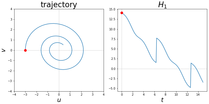
Figure 1: Plots of a trajectory and the corresponding values of the purported constant $H_{1}$, due to Liu, et al. Liu et al. (2022b). Of note is that $H_{1}$ is not actually a constant. Here $\arctan(p/x)$ was instead computed using arctan2(p,x) from the Numpy library Num (2023). The red dot indicates the starting point.

In the left plot of the figure is shown the trajectory for $t\in[0,14.9]$, with a red dot indicating the initial value; corresponding values of $H_{1}$ are shown in the right plot. This clearly shows that their $H_{1}$ is not a constant.

In summary, they obtained an incorrect result using an incorrect method; if their method is corrected, it can no longer be used.

Afterword

Intermediate steps: The reader should note that some of the work summarized in the Review portion has a counterpart in the earlier work of Zimmer (Zimmer, 2021). For example, Eqs. 3,4 in this Comment can be matched to similar equations in App. C of (Zimmer, 2021). (The author has since streamlined his approach in his latest preprint (Zimmer, 2024), and now uses different intermediate steps.)

Their analytical approach: In their treatment of the 1D damped oscillator, they began from exact solutions for $x,p$, and then formed combinations of them to isolate the parameters of the solution, thereby determining a constant of motion. Such an approach can only be used, as they presented it, in the undamped case. To make it work in the damped case, they should have made a variable change ($x\rightarrow w=\gamma x+p$) that Zimmer recognized (see App. D.2 of (Zimmer, 2024)). However, Liu, et al. gave no indication they were aware of such a transformation.

2D oscillator: Liu, et al. also analyzed the 2D oscillator (undamped), and made similar omissions regarding Riemann sheets, as they did in the 1D case. However, most notable is that they did not express their constant as a function of $x,p$ (i.e., in terms of “$\tan^{-1}$”); they instead kept it as a function of the solution parameters. They thus missed the chance to see how such a result could be used as a generalization of angular momentum, as well as other results (see Secs. VI E-G in (Zimmer, 2024)). Also, they would then go on to to write the following pejorative remarks, which the author disagrees with: (1) in the caption of Fig. 5 on p. 045307-7, “an everywhere discontinuous function that is completely useless to physicists”; (2) on p. 045307-6, “ill-behaved, demonstrating fractal behavior”. The author suggests the latter may be a graphical aliasing effect.

References

- Zimmer (2021) M. F. Zimmer, arXiv preprint arXiv:2110.06917v2 (2021), (See Appendix C).
- Liu et al. (2022a) Z. Liu, V. Madhavan, and M. Tegmark, arXiv preprint arxiv:2203.12610 (2022a).
- Liu et al. (2022b) Z. Liu, V. Madhavan, and M. Tegmark, Phys. Rev. E 106, 045307 (2022b).
- Rainville and Bedient (1981) E. D. Rainville and P. E. Bedient, Elementary Differential Equations, 6th ed. (Macmillan Publishing Co., 1981).
- MIT Open Courseware (2011) MIT Open Courseware, “Differential equations (18.03sc),” (2011).
- Olver and Shakiban (2006) P. J. Olver and C. Shakiban, Applied Linear Algebra, 2nd ed. (Springer, 2006).
- Wikipedia contributors (2024) Wikipedia contributors, “Complex logarithm,” (2024), [Online accessed April 2, 2024].
- Num (2023) Numpy API Reference, arctan2 (numpy.org) (2023).
- Zimmer (2024) M. F. Zimmer, arXiv preprint arXiv:2403.19418 (2024).