Linear Attention Sequence Parallelism

Abstract

Sequence Parallel (SP) serves as a prevalent strategy to handle long sequences that exceed the memory limit of a single GPU. However, existing SP methods do not take advantage of linear attention features, resulting in sub-optimal parallelism efficiency and usability for linear attention-based language models. In this paper, we introduce Linear Attention Sequence Parallel (LASP), an efficient SP method tailored to linear attention-based language models. Specifically, we design an efficient point-to-point communication mechanism to leverage the right-product kernel trick of linear attention, which sharply decreases the communication overhead of SP. We also enhance the practical efficiency of LASP by performing kernel fusion and intermediate state caching, making the implementation of LASP hardware-friendly on GPU clusters. Furthermore, we meticulously ensure the compatibility of sequence-level LASP with all types of batch-level data parallel methods, which is vital for distributed training on large clusters with long sequences and large batches. We conduct extensive experiments on two linear attention-based models with varying sequence lengths and GPU cluster sizes. LASP scales sequence length up to 4096K using 128 A100 80G GPUs on 1B models, which is 8$\times$ longer than existing SP methods while being significantly faster. The code is available at https://github.com/OpenNLPLab/LASP.

1 Introduction

Recently, linear attention-based models (Qin et al., 2024a, 2022a; Choromanski et al., 2020) are becoming increasingly popular due to their faster processing speed and comparable language modeling performance to vanilla Softmax transformers (Vaswani et al., 2017). Meanwhile, the growing size of large language models (LLMs) (Touvron et al., 2023a, b; Tang et al., 2024) and longer sequence lengths exert significant strain on contemporary GPU hardware because the memory of a single GPU confines the maximum sequence length of a language model. To tackle this issue, the Sequence Parallelism (SP) techniques (Li et al., 2022; Korthikanti et al., 2022) are often utilized to divide a long sequence into several sub-sequences and train them on multiple GPUs separately. Unfortunately, existing SP methods do not fully leverage the benefits of linear attention features, leading to suboptimal parallelism efficiency and usability.

In this paper, we present the Linear Attention Sequence Parallel (LASP) technique for efficient sequence parallelism on linear transformers. Our approach includes a sophisticated communication mechanism based on point-to-point (P2P) communication for exchanging intermediate states during forward and backward passes among GPUs within a node or across multiple nodes. This design maximizes the utilization of right-product kernel tricks (Katharopoulos et al., 2020; Qin et al., 2023b, 2024b) in linear attention. Notably, our technique is independent of attention heads partitioning, which allows it to be applied to models with varying numbers or styles of attention heads, such as multi-head, multi-query, and grouped-query attentions. This flexibility exceeds the capabilities of existing SP methods in Megatron-LM (Shoeybi et al., 2019; Korthikanti et al., 2022) or DeepSpeed (Jacobs et al., 2023).

Our implementation of LASP incorporates system engineering optimizations such as kernel fusion and KV State caching, resulting in significantly enhanced execution efficiency. Furthermore, we have taken care in ensuring compatibility of LASP with various (sharded) distributed data-parallel (DDP) (Li et al., 2020; Sun et al., 2024) training methods during the implementation, which we refer to as the data-sequence hybrid parallelism. Through extensive experiments with models of different parameters, cluster sizes, and sequence lengths, we demonstrate LASP’s impressive performance and efficiency when used with these DDP instances. Specifically, LASP is significantly faster than existing SP methods and can extend sequence length 8$\times$ longer under the same hardware constraints.

Our primary contributions can be summarized as follows:

• A new SP strategy that is tailored to linear attention. Enabling linear attention-based models to scale for long sequences without being limited by a single GPU.

• Sequence length-independent communication overhead. Our elegant communication mechanism leverages right-product kernel trick of linear attention to ensure that the exchanging of linear attention intermediate states is sequence length-independent.

• GPU friendly implementation. We optimize LASP’s execution on GPUs through meticulous system engineering, including kernel fusion and KV State caching.

• Data-parallel compatibility. LASP is compatible with all batch-level DDP methods, such as PyTorch/Legacy DDP, FSDP, and ZeRO-series optimizers.

2 Method

2.1 Preliminary

Softmax Attention. Consider the standard attention  (Vaswani et al., 2017) computation with causal masking in the transformer architecture, formulated as:

$$\small\mathbf{O}=\mathrm{Softmax}(\mathbf{Q}\mathbf{K}^{\top}/\sqrt{d}\odot\mathbf{M})\mathbf{V},$$ (1)

where $d$ denotes the hidden dimension. The matrices $\mathbf{Q},\mathbf{K},\mathbf{V}\in\mathbb{R}^{N\times d}$ represent query, key, and value matrices, respectively. These matrices are linear projections of the input $\mathbf{X}\in\mathbb{R}^{N\times d}$, i.e., $\mathbf{Q}=\mathbf{X}\mathbf{W_{Q}}$, $\mathbf{K}=\mathbf{X}\mathbf{W_{K}}$, $\mathbf{V}=\mathbf{X}\mathbf{W_{V}}$. The output matrix is denoted as $\mathbf{O}\in\mathbb{R}^{N\times d}$, and $\mathbf{M}\in\mathbb{R}^{N\times N}$ represents the causal mask matrix. The $\mathrm{Softmax(\cdot)}$ operation introduces quadratic time complexity relative to the input sequence length $N$, limiting the scalability of vanilla transformers to extended input sequences.

Linear Attention. Linear attention is originally proposed in (Katharopoulos et al., 2020), with the elimination of Softmax operation (Vaswani et al., 2017). Qin et al. (2022a, 2023a) propose to replace the Softmax operation with a normalization operation $\mathrm{Norm(\cdot)}$, which turns to a concise formulation as:

$$\small\mathbf{O}=\mathrm{Norm}((\mathbf{Q}\mathbf{K}^{\top}\odot\mathbf{M})\mathbf{V}).$$ (2)

When considering bidirectional tasks, the above formulation can be simplified as $\mathbf{O}=\mathrm{Norm}((\mathbf{Q}\mathbf{K}^{\top})\mathbf{V})$. Then by performing the associativity property of matrix products, it can be mathematically equivalently transformed into a right-product version:

$$\small\mathbf{O}=\mathrm{Norm}(\mathbf{Q}(\mathbf{K}^{\top}\mathbf{V})).$$ (3)

This linear attention formulation facilitates recurrent prediction with a computational complexity of $O(Nd^{2})$. And the recurrent update of $\mathbf{K}^{\top}\mathbf{V}$ without needing to compute the entire attention matrix makes its inference efficient.

While linear complexity offers significant advantages in terms of computational efficiency and memory optimization for linear attention, it still incurs a proportional increase in computation and memory utilization on a single GPU as the sequence length $N$ grows. This can lead to memory constraints on a single GPU, such as the 80GB limit in NVIDIA A100, for exceptionally long sequences. The challenge of achieving zero-redundancy (on sequence level) training for such long sequences using linear attention-based LLMs across GPU clusters remains an open problem. Furthermore, the complexity of addressing this issue in a casual setting further intensifies the challenge. To address this, we propose LASP as a solution for parallelizing linear attention training at the sequence level, even in a casual setting.

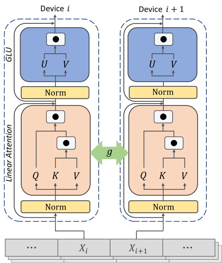
Figure 1: Visualization of LASP. We illustrate a typical linear transformer layer to explain the mechanism of LASP. $\mathbf{X}$ as an input sequence is partitioned into multiple sub-sequence chunks, which are then fed into different model copies on discrete devices. $g$ represents conjugate communication operations in forward and backward passes. In forward pass, $g$ is Send $\&$ Recv from device $i$ to $(i+1)$. While in backward pass, $g$ is Send $\&$ Recv from device $(i+1)$ to $i$. The communication operations exchange intermediate states $\mathbf{KV}$ and $\mathbf{dKV}$ during forward and backward passes to insure the performance of SP.

2.2 LASP

LASP tiles sequence over the cluster. Follow the thought-of-tiling, LASP partitions the input sequences into multiple sub-sequence chunks, distributing these chunks individually across different GPUs. For linear attention in a casual setting, in order to fully exploit the advantage of right-product in linear attention, we categorize the attention computation for sub-sequences into two distinct types: intra-chunks and inter-chunks. Intra-chunks involve conventional attention computation, while inter-chunks leverage the kernel tricks associated with linear attention’s right-product. Further details regarding the intricate mechanisms of LASP in data distribution, forward pass, and backward pass are expounded upon below. A visualization of LASP is presented in Fig. 1.

Data Distribution.

LASP is designed for training long sequences on linear transformers in a distributed environment, achieved by partitioning the input data along its sequence dimension. In this situation, each GPU within the distributed environment undertakes the training of a subset of sub-sequences, which serves to diminish the large memory footprint associated with activation during the training of long sequences. Communication operations are introduced between GPUs to transmit intermediate states. The final trained model assimilates the knowledge derived from the entirety of the long sequences.

For an input sequence of length $N$, we establish its embedding space representation denoted as $\mathbf{X}\in\mathbb{R}^{N\times d}$ with a feature dimension of $d$. In the LASP framework, $\mathbf{X}$ is evenly partitioned into $T$ chunks, where $T$ is called the sequence parallel size, which must be divisible by the distributed world size $W$. These segmented data chunks are subsequently assigned to the respective GPUs. It is essential to note that different sequence parallel groups receive dissimilar data batches. However, within the same group, all data chunks originate from an identical batch of data. A comprehensive depiction of the data distribution process in LASP is provided in Algorithm 1. Additionally, an illustrative example of data distribution in LASP is presented in Fig. 2, considering a node with 8 GPUs and the partitioning of 2 sequences into 4 sub-sequence chunks.

Algorithm 1 LASP Data Distribution

1:  Input: An input sequence in embedding space $\mathbf{X}\in\mathbb{R}^{N\times d}$ with sequence length $N$ and hidden dimension $d$, distributed world size $W$ and sequence parallel size $T$.

2:  Obtain number of sequence parallel groups $G=W/T$.

3:  Obtain sub-sequence length (or chunk size) $C=N/T$.

4:  Get global rank list $R=\text{get\_global\_rank}()$.

5:  Obtain sequence parallel source rank list $R_{{src}}=\lfloor R/T\rfloor*T$.

6:  Along sequence dimension, split $\mathbf{X}$ into $T$ chunks $\{\mathbf{X}_{1},\mathbf{X}_{2},...\mathbf{X}_{T}\}$, of size $C\times d$ for each.

7:  Transfer copies of data chunks $\{\mathbf{X}_{1},\mathbf{X}_{2},\cdots,\mathbf{X}_{T}\}$ to GPUs with rank indices in $R_{src}$.

8:  Scatter $\{\mathbf{X}_{1},\mathbf{X}_{2},\cdots,\mathbf{X}_{T}\}$ from $R_{src}$ to all ranks in respective sequence parallel groups.

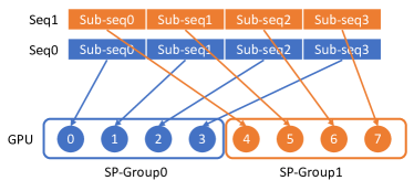
Figure 2: Example of LASP Data Distribution. In this illustration, the distributed world size is characterized by $W=8$, the sequence parallel size by $T=4$, the number of sequence parallel groups by $G=2$, and the sequence parallel source rank list by $R_{{src}}=[0,4]$. For the first batch Seq0, the input sequence ${\mathbf{X}}$ undergoes partitioning into $T$ chunks $\{\mathbf{X}_{1},\mathbf{X}_{2},...\mathbf{X}_{T}\}$ along the sequence dimension, subsequently transmitted to the first rank in the first SP group denoted as SP-Group0, which corresponds to global rank 0. The data chunks on global rank 0 are then scattered to global ranks 0, 1, 2, 3 within SP-Group0, where each rank only retains a single chunk. The subsequent batch Seq1 follows a similar allocation procedure, being assigned to global ranks 4, 5, 6, 7 within SP-Group1.

Algorithm 2 LASP Forward Pass

1:  Input: input sequence in embedding space $\mathbf{X}\in\mathbb{R}^{N\times d}$ with sequence length $N$ and hidden dimension $d$, distributed world size $W$, sequence parallel size $T=W$, decay rate $\lambda\in\mathbb{R}^{+}$.

2:  Distribute input sequence $\mathbf{X}$ according to Algorithm 1.

3:  Obtain sub-sequence length (or chunk size) $C=N/T$.

4:  Initialize mask $\mathbf{M}\in\mathbb{R}^{C\times C}$, where $M_{ij}=\lambda^{i-j}$, if $i\geq j$, else $M_{ij}=0$.

5:  Initialize $\mathbf{\Lambda}=\mathrm{diag}\{\lambda,\lambda^{2},\cdots,\lambda^{C}\}\in\mathbb{R}^{C\times C}$.

6:  Initialize activation state $\mathbf{KV}=\mathbf{0}\in\mathbb{R}^{d\times d}$.

7:  for chunk $t\in\{1,\cdots,T\}$ at rank $i\in\{1,\cdots,W\}$ in parallel do

8:    Calculate $\mathbf{Q}_{t}=\mathbf{X}_{t}\mathbf{W}_{Q}$, $\mathbf{K}_{t}=\mathbf{X}_{t}\mathbf{W}_{K}$, $\mathbf{V}_{t}=\mathbf{X}_{t}\mathbf{W}_{V}$ according to its own data chunk, of size $C\times d$ for each.

9:    Compute $\mathbf{O}_{\mathrm{t,intra}}=[(\mathbf{Q}_{t}\mathbf{K}_{t}^{\top})\odot\mathbf{M}]\mathbf{V}_{t}$.

10:  end for

11:  for chunk $t\in\{1,\cdots,T\}$ at rank $i\in\{1,\cdots,W\}$ do

12:    Recv activation $\mathbf{KV}_{t-1}$ from rank $(i-1)$.

13:    Save $\mathbf{KV}_{{t-1}}$ as $\mathbf{KV}_{i}$ on rank $i$ for backward computation.

14:    Compute $\mathbf{O}_{\mathrm{t,inter}}=\mathbf{\Lambda}\mathbf{Q}_{t}\mathbf{KV}_{t-1}$.

15:    Compute $\mathbf{O}_{t}=\mathbf{O}_{\mathrm{t,intra}}+\mathbf{O}_{\mathrm{t,inter}}$ as $\mathbf{O}$ of $t$-th chunk.

16:    Update $\mathbf{KV}_{{t}}=\lambda^{C}\mathbf{KV}_{{t-1}}+(\lambda^{C}\mathbf{\Lambda}^{-1}\mathbf{K}_{t})^{\top}\mathbf{V}_{t}$.

17:    Send activation $\mathbf{KV}_{{t}}$ to rank $(i+1)$.

18:  end for

19:  return $\mathbf{O}=[\mathbf{O}_{t}]$, with $t\in\{1,\cdots,T\}$.

Forward Pass.

To streamline derivations, the $\mathrm{Norm}(\cdot)$ operator in Eq. (2) is temporarily omitted. Additionally, we consider a normal case where $W=T$, indicating $G=W/T=1$. In this scenario, GPU with rank $0$ consolidates all split sub-sequences in a batch, subsequently distributing them to all GPUs across the entire distributed world. It is noteworthy that the scenario where the sequence parallel size is not equal to world size is discussed in 2.5.

We first define two symbols $\mathbf{kv}$ and $\mathbf{KV}$ which are important in the right-product computation procedure of linear attention. Without loss of generality, we add $\lambda$ as the decay rate in linear attention with casual mask, choosing $\lambda=1$ yields the ordinary linear attention. In the forward pass of linear attention computation with casual mask, the $s$-th output can be formulated as

$$\small\mathbf{o}_{s}^{\top}=\mathbf{q}_{s}^{\top}\sum_{i\leq s}\lambda^{s-i}\mathbf{k}_{i}\mathbf{v}_{i}^{\top}.$$ (4)

Rewrite in a recursive form (Katharopoulos et al., 2020), we have

$$\mathbf{kv}_{0} =0\in\mathbb{R}^{d\times d},$$ (5)

$$\mathbf{kv}_{s} =\lambda\mathbf{kv}_{s-1}+\mathbf{k}_{s}\mathbf{v}_{s}^{\top},$$

$$\mathbf{o}_{s}^{\top} =\mathbf{q}_{s}^{\top}(\mathbf{kv}_{s}),$$

where

$$\small\textstyle\mathbf{kv}_{s}=\sum_{i\leq s}\lambda^{s-i}\mathbf{k}_{i}\mathbf{v}_{i}^{\top}$$ (6)

is the activation state in the forward computation of linear attention with $s$-th input.

In the sequence parallelism scenario, given data chunk $\mathbf{X}_{t}$ on rank $i$, the query, key and value corresponding to $\mathbf{X}_{t}$ is $\mathbf{Q}_{t}=\mathbf{X}_{t}\mathbf{W}_{Q}$, $\mathbf{K}_{t}=\mathbf{X}_{t}\mathbf{W}_{K}$, $\mathbf{V}_{t}=\mathbf{X}_{t}\mathbf{W}_{V}$. Note that we assume $T=W$ here, their indices are thus equivalent, i.e., $t=i$. The output within the $t$-th chunk can be calculated as

$$\small\mathbf{O}_{\mathrm{t,intra}}=[(\mathbf{Q}_{t}\mathbf{K}_{t}^{\top})\odot\mathbf{M}]\mathbf{V}_{t}.$$ (7)

The intra-chunk computation has no dependencies with other chunks on other GPUs, so it can be calculated parallelized on all ranks in the distributed world. However, this result does not consider the impact of the previous $1\sim(t-1)$ chunks on the $t$-th chunk, which is called an inter-chunk. To calculate inter-chunk, let us rearrange Eq. (4) as

$$\mathbf{o}_{s+C}^{\top}=\mathbf{q}_{s+C}^{\top}\sum_{i\leq s+C}\lambda^{s+C-i}\mathbf{k}_{i}\mathbf{v}_{i}^{\top}$$ (8)

$$= \mathbf{q}_{s+C}^{\top}\sum_{i=C+1}^{C+s}\lambda^{s+C-i}\mathbf{k}_{i}\mathbf{v}_{i}^{\top}+\lambda^{s}\mathbf{q}_{s+C}^{\top}\sum_{i\leq C}\lambda^{C-i}\mathbf{k}_{i}\mathbf{v}_{i}^{\top}.$$

The first part (before the plus sign) in Eq. (8) corresponds to the computation on intra-chunk, and the second part (after the plus sign) corresponds to the computation on inter-chunk. In sequence parallelism scenario, Eq. (8) can be rewritten in the chunk form as follows:

$$\small\mathbf{O}_{\mathrm{t,inter}}=\bm{\Lambda}\mathbf{Q}_{t}\mathbf{K}\mathbf{V}_{t-1},$$ (9)

where

$$\small\mathbf{KV}_{t}=\mathbf{kv}_{tC}.$$ (10)

It is worth noting that the calculation of the inter part for the $t$-th chunk depends on the activation state of previous $(t-1)$ chunk, i.e., $\mathbf{KV}_{t-1}$, which is calculated on rank $(i-1)$. Thus a P2P communication operation Recv should be performed to pull $\mathbf{KV}_{t-1}$ from rank $(i-1)$ to rank $i$. Then the activation state $\mathbf{KV}_{t}$ should be updated for subsequent inter-chunk attention computation at $(t+1)$-th chunk. The update rule of $\mathbf{KV}_{t}$ at $t$-th chunk is

$$\mathbf{KV}_{t} =\sum_{s\leq tC}\lambda^{tC-s}\mathbf{k}_{s}\mathbf{v}_{s}^{\top}$$ (11)

$$=\lambda^{C}\!\!\!\!\sum_{s\leq(t-1)C}\!\!\!\!\lambda^{(t-1)C-s}\mathbf{k}_{s}\mathbf{v}_{s}^{\top}+\!\!\!\!\!\!\sum_{s=(t-1)C+1}^{tC}\!\!\!\!\!\!\lambda^{tC-s}\mathbf{k}_{s}\mathbf{v}_{s}^{\top}$$

$$=\lambda^{C}\mathbf{KV}_{t-1}+\left(\mathrm{diag}\{\lambda^{C-1},\ldots,1\}\mathbf{K}_{t}\right)^{\top}\mathbf{V}_{t}$$

$$=\lambda^{C}\mathbf{KV}_{t-1}+\left(\lambda^{C}\mathbf{\Lambda}^{-1}\mathbf{K}_{t}\right)^{\top}\mathbf{V}_{t}.$$

In correspondence to the preceding Recv operation, another P2P communication operation Send is executed to transmit the acquired $\mathbf{KV}_{t}$ in Eq. (11) to the subsequent rank $(i+1)$ for its inter-chunk computation.

It is noteworthy that in the backward pass, the $t$-th chunk necessitates $\mathbf{KV}_{t-1}$ as activation to calculate gradients. To minimize communication operations, we cache $\mathbf{KV}_{t-1}$ on High-Bandwidth Memory (HBM) to accelerate computation. Integrating both the intra and inter parts, the final forward output is as follows:

$$\small\mathbf{O}_{t}=\mathbf{O}_{t,\mathrm{intra}}+\mathbf{O}_{t,\mathrm{inter}}$$ (12)

We present the complete expression of forward pass for LASP with $W=T$ in Algorithm 2.

Algorithm 3 LASP Backward Pass

1:  Input: Sequence Length $N$, Distributed world size $W$, sequence parallel size $T$, decay rate $\lambda\in\mathbb{R}^{+}$, $\mathbf{Q}_{t},\mathbf{K}_{t},\mathbf{V}_{t},\mathbf{O}_{t},\mathbf{dO}_{t}\in\mathbb{R}^{C\times d}$ for $t\in\{1,2,\cdots,{T}\}$.

2:  Obtain sub-sequence length (or chunk size) $C=N/T$.

3:  Initialize mask $\mathbf{M}\in\mathbb{R}^{C\times C}$, where $M_{ij}=\lambda^{i-j}$, if $i\geq j$, else $M_{ij}=0$.

4:  Initialize $\mathbf{\Lambda}=\mathrm{diag}\{\lambda,\lambda^{2},\cdots,\lambda^{C}\}\in\mathbb{R}^{C\times C}$ .

5:  Initialize $\mathbf{dKV}=\mathbf{0}\in\mathbb{R}^{d\times d}$.

6:  for $t\in\{1,2,\cdots,T\}$ at rank $i\in\{1,2,\cdots,W\}$ in parallel do

7:    Compute $\mathbf{dQ}_{\mathrm{t,intra}}=[(\mathbf{dO}_{t}\mathbf{V}_{t}^{\top})\odot\mathbf{M}]\mathbf{K}_{t}$.

8:    Compute $\mathbf{dQ}_{\mathrm{t,inter}}=\mathbf{\Lambda}\mathbf{dO}_{t}\mathbf{KV}_{t-1}^{\top}$.

9:    Compute $\mathbf{dK_{\mathrm{t,intra}}}=[(\mathbf{dO}_{t}\mathbf{V}_{t}^{\top})\odot\mathbf{M}]^{\top}\mathbf{Q}_{t}$.

10:    Compute $\mathbf{dV_{\mathrm{t,intra}}}=[(\mathbf{Q}_{t}\mathbf{K}_{t}^{\top})\odot\mathbf{M}]^{\top}\mathbf{dO}_{t}$.

11:  end for

12:  for $t\in\{T,\cdots,2,1\}$ at rank $i\in\{W,\cdots,2,1\}$ do

13:    Recv activation $\mathbf{dKV}_{t+1}$ from rank $(i+1)$.

14:    Compute $\mathbf{dK_{\mathrm{t,inter}}}={(\lambda^{C}\mathbf{\Lambda}^{-1}\mathbf{V}_{t})}\mathbf{dKV}_{t+1}^{\top}$.

15:    Compute $\mathbf{dV_{\mathrm{t,inter}}}=(\lambda^{C}\mathbf{\Lambda}^{-1}\mathbf{K}_{t})\mathbf{dKV}_{t+1}$.

16:    Load $\mathbf{KV}_{i}$ as $\mathbf{KV}_{t}$ on rank $i$.

17:    Combine intra- and inter-chunks of $\mathbf{dQ}_{t},\mathbf{dK}_{t},\mathbf{dV}_{t}$:

$$\mathbf{dQ}_{t} =\mathbf{dQ}_{t,\mathrm{intra}}+\mathbf{dQ}_{t,\mathrm{inter}},$$

$$\mathbf{dK}_{t} =\mathbf{dK}_{t,\mathrm{intra}}+\mathbf{dK}_{t,\mathrm{inter}},$$

$$\mathbf{dV}_{t} =\mathbf{dV}_{t,\mathrm{intra}}+\mathbf{dV}_{t,\mathrm{inter}}.$$

18:    Compute $\mathbf{dKV}_{t}=\lambda^{C}\mathbf{dKV}_{t+1}+(\mathbf{\Lambda}\mathbf{Q}_{t})^{\top}\mathbf{dO}_{t}$.

19:    Send activation $\mathbf{dKV}_{t}$ to rank $i$.

20:  end for

21:  return $\mathbf{dQ}=[\mathbf{dQ}_{t}]$, $\mathbf{dK}=[\mathbf{dK}_{t}]$, $\mathbf{dV}=[\mathbf{dV}_{t}]$, with $t\in\{1,2,\cdots,T\}$.

Backward Pass.

For the backward pass, let us examine the inverse procedure. We first define $\mathbf{dkv}_{t}$ for subsequent analysis. Given $\mathbf{do}_{s}$, we have (Katharopoulos et al., 2020)

$$\mathbf{dq}_{s}^{\top} =\mathbf{do}_{s}^{\top}\mathbf{kv}_{s}^{\top}\in\mathbb{R}^{1\times d},$$ (13)

$$\mathbf{dk}_{s}^{\top} =\mathbf{v}_{s}^{\top}\mathbf{dkv}_{s}^{\top}\in\mathbb{R}^{1\times d},$$

$$\mathbf{dv}_{s}^{\top} =\mathbf{k}_{s}^{\top}\mathbf{dkv}_{s}\in\mathbb{R}^{1\times d},$$

$$\mathbf{dkv}_{s} =\sum_{i\geq s}\lambda^{i-s}\mathbf{q}_{i}\mathbf{do}_{i}^{\top}\in\mathbb{R}^{d\times d}.$$

By writing $\mathbf{dkv}_{s}$ in a recursive form, we have

$$\mathbf{dkv}_{n+1} =0\in\mathbb{R}^{d\times d},$$ (14)

$$\quad\mathbf{dkv}_{s-1} =\lambda\mathbf{dkv}_{s}+\mathbf{q}_{s-1}\mathbf{do}_{s-1}^{\top}.$$

In the sequence parallelism scenario, we have $\{\mathbf{Q_{t}},\mathbf{K_{t}},\mathbf{V_{t}},\mathbf{O_{t}},\mathbf{dO_{t}}\}$ which corresponds to the $t$-th sub-sequence chunk on rank $i$, where $t\in\{1,\cdots,T\}$ and $i\in\{1,\cdots,W\}$. Same with the forward pass, the following derivations assume $t=i$, $T=W$.

We first calculate $\mathbf{dQ}$ with respective to the $t$-th data chunk, which yields:

$$\small\mathbf{dQ}_{t,\mathrm{intra}}=[(\mathbf{dO}_{t}\mathbf{V}_{t}^{\top})\odot\mathbf{M}]\mathbf{K}_{t}.$$ (15)

Since the computation of $\mathbf{dQ}_{t,\mathrm{intra}}$ is independent, its calculation can be parallelized on all GPUs. While the calculation of $\mathbf{dQ}_{t,\mathrm{inter}}$ reflects the inter-dependence of chunks $1$ to $t-1$ on chunk $t$. In order to compute the inter part, we transform Eq. (13) as

$$\mathbf{dq}_{s+C}^{\top}=\mathbf{do}_{s+C}^{\top}\sum_{i\leq s+C}\lambda^{s+C-i}\mathbf{v}_{i}\mathbf{k}_{i}^{\top}$$ (16)

$$= \mathbf{do}_{s+C}^{\top}\sum_{i=C+1}^{C+s}\lambda^{s+C-i}\mathbf{v}_{i}\mathbf{k}_{i}^{\top}+\lambda^{s}\mathbf{do}_{s+C}^{\top}\sum_{i\leq C}\lambda^{C-i}\mathbf{v}_{i}\mathbf{k}_{i}^{\top}.$$

The first part (before the plus sign) in Eq. (16) corresponds to the intra-chunk, while the second part (after the plus sign) corresponds to the inter-chunk. In sequence parallelism scenario, we can calculate $\mathbf{dQ}_{t,\mathrm{inter}}$ as

$$\small\mathbf{dQ}_{t,\mathrm{inter}}=\mathbf{\Lambda}\mathbf{dO}_{t}\mathbf{KV}_{t-1}^{\top}.$$ (17)

Note that $\mathbf{KV}_{t}$ has already been computed and cached during the forward pass, so no communication is required here to obtain $\mathbf{KV}_{t}$. Benefit from the $\mathbf{KV}$ state caching, the calculation of $\mathbf{dQ}_{t,\mathrm{inter}}$ can also be executed in parallel.

Next, let us take $\mathbf{dK}$ into consideration, $\mathbf{dK}$ within the $t$-th chunk can be calculated in parallel as

$$\small\mathbf{dK}_{t,\mathrm{intra}}=[(\mathbf{dO}_{t}\mathbf{V}_{t}^{\top})\odot\mathbf{M}]^{\top}\mathbf{Q}_{t}.$$ (18)

Then we transform Eq. (13) as

$$\mathbf{dk}_{s}^{\top}=\mathbf{v}_{s}^{\top}\sum_{i\geq s}\lambda^{i-s}\mathbf{do}_{i}\mathbf{q}_{i}^{\top}$$ (19)

$$= \mathbf{v}_{s}^{\top}\sum_{i=s}^{C}\lambda^{i-s}\mathbf{do}_{i}\mathbf{q}_{i}^{\top}+\lambda^{C-s}\mathbf{v}_{s}^{\top}\sum_{i\geq C+1}\lambda^{i-C}\mathbf{do}_{i}\mathbf{q}_{i}^{\top},$$

where the first term (before the plus sign) corresponds to the intra-chunk, and the second term (after the plus sign) corresponds to the inter-chunk. The above equation can be rewritten in terms of chunks as follow:

$$\small\mathbf{dK}_{t,\mathrm{inter}}=\lambda^{C}\mathbf{\Lambda}^{-1}\mathbf{V}_{t}\mathbf{dKV}_{t+1}^{\top}.$$ (20)

Here a Recv operation is required here to pull $\mathbf{dKV}_{t+1}$ from the $(t+1)$-th chunk. Then in order to compute $\mathbf{dKV}$ for the $(t-1)$-th chunk, $\mathbf{dKV}$ should be updated as:

$$\mathbf{dKV}_{t} =\sum_{s>tC}\lambda^{s-tC}\mathbf{q}_{s}\mathbf{do}_{s}^{\top}$$ (21)

$$=\lambda^{C}\!\!\!\!\sum_{s>(t+1)C}\!\!\!\!\lambda^{s-(t+1)C}\mathbf{q}_{s}^{\top}\mathbf{do}_{s}+\!\!\!\!\sum_{s=tC+1}^{(t+1)C}\!\!\!\!\lambda^{s-tC}\mathbf{q}_{s}\mathbf{do}_{s}^{\top}$$

$$=\lambda^{C}\mathbf{dKV}_{t+1}+\left(\mathbf{\Lambda}\mathbf{Q}_{t}\right)^{\top}\mathbf{dO}_{t}.$$

Then a Send operation is performed to push $\mathbf{dKV}_{t}$ to rank $(i-1)$.

Finally, for $\mathbf{dV}$, its intra part can be calculated as

$$\small\mathbf{dV}_{t,\mathrm{intra}}=[(\mathbf{Q}_{t}\mathbf{K}_{t}^{\top})\odot\mathbf{M}]^{\top}\mathbf{dO}_{t}.$$ (22)

Again we transform Eq. (13) as:

$$\mathbf{dv}_{s}^{\top}=\mathbf{k}_{s}^{\top}\sum_{i\geq s}\lambda^{i-s}\mathbf{q}_{i}\mathbf{do}_{i}^{\top}$$ (23)

$$= \mathbf{k}_{s}^{\top}\sum_{i=s}^{C}\lambda^{i-s}\mathbf{q}_{i}\mathbf{do}_{i}^{\top}+\lambda^{C-s}\mathbf{k}_{s}^{\top}\sum_{i\geq C+1}\lambda^{i-C}\mathbf{q}_{i}\mathbf{do}_{i}^{\top}.$$

The first and second terms (before and after the plus sign) corresponds to the computation of the intra- and inter-chunks, respectively. In sequence parallelism, $\mathbf{dV}_{t,\mathrm{inter}}$ can be calculated as:

$$\small\mathbf{dV}_{t,\mathrm{inter}}=\lambda^{C}\mathbf{\Lambda}^{-1}\mathbf{K}_{t}\mathbf{dKV}_{t+1}.$$ (24)

Combine the intra and inter part, we obtain the final results of $\mathbf{dQ}_{t}$, $\mathbf{dK}_{t}$ and $\mathbf{dV}_{t}$:

$$\mathbf{dQ}_{t} =\mathbf{dQ}_{t,\mathrm{intra}}+\mathbf{dQ}_{t,\mathrm{inter}},$$ (25)

$$\mathbf{dK}_{t} =\mathbf{dK}_{t,\mathrm{intra}}+\mathbf{dK}_{t,\mathrm{inter}},$$

$$\mathbf{dV}_{t} =\mathbf{dV}_{t,\mathrm{intra}}+\mathbf{dV}_{t,\mathrm{inter}}.$$

We provide the comprehensive formulation of the backward pass for LASP with $W=T$ in Algorithm 3.

2.3 Communication Analysis

Table 1: Communication Volume Comparison. Last column: we eliminate the common factors $Bd$ for ease of comparison.

Method	Full Formulation	Simplified Formulation
LASP	$Bd^{2}/h$	$d/h$
DeepSpeed-Ulysses	$4BNd/T$	$4N/T$
Megatron-SP	$2BNd+4BNd/T$	$2N+4N/T$

When examining the LASP algorithm, it is important to note that the forward pass requires communication for the $\mathbf{KV}$ activation in each linear attention module layer. The communication volume is determined by $Bd^{2}/h$, where $B$ is the batch size and $h$ is the number of heads. In comparison, sequence parallelism in Megatron-LM utilizes all-gather operations twice after two layer normalization layers within each transformer layer, and a reduce-scatter operation after the attention and Feedforward Neural Network (FFN) layers. This results in a communication volume of $2BNd+4BNd/T$. DeepSpeed uses all-to-all collective communication operation (Thakur et al., 2005) for input $\mathbf{Q},\mathbf{K},\mathbf{V}$, and output $\mathbf{O}$ of each attention module layer, resulting in a communication volume of $4BNd/T$.

Table 1 displays a comparison of communication volumes across three frameworks. $d/h$ is the head dimension which is set at 128 as usual  (Lan et al., 2020). In practical applications where $N/T\geq 32$, LASP is able to achieve the lowest theoretical communication volume. Furthermore, the communication volume of LASP is not impacted by changes in sequence length $N$ or sub-sequence length $C$, which is a huge advantage for extremely long sequence parallelism across large GPU clusters.

2.4 System Engineering Optimization

Kernel Fusion. To improve the efficiency of LASP on GPU, we perform kernel fusion in both the intra-chunk and inter-chunk computations, and also fused the updates of $\mathbf{KV}$ and $\mathbf{dKV}$ into the intra-chunk and inter-chunk computations.

$\mathbf{KV}$ State Caching. To avoid recomputing activation $\mathbf{KV}$ during the backward pass, we choose to store it in the HBM of the GPU right after computing it in the forward pass. During the subsequent backward pass, LASP directly accesses $\mathbf{KV}$ for use. It is important to note that the size of the $\mathbf{KV}$ activation cached in HBM is $d\times d$, which is not affected by the sequence length $N$. When the input sequence length $N$ is exceptionally large, the memory usage of $\mathbf{KV}$ becomes insignificant.

2.5 Data-Sequence Hybrid Parallelism

The technique of Data Parallelism is commonly used to split input data along the batch dimension for large-scale distributed deep learning. However, LASP offers a different approach by dividing data along the sequence dimension, which makes it easier to integrate with Data Parallelism. As explained in Section 2.2 and illustrated in Fig. 2, LASP allows for the specification of a smaller sequence parallel size that is divisible by the distributed world size. This configuration results in the input data being split along both the batch and sequence dimensions, which is a type of hybrid parallelism called data-sequence hybrid parallelism.

Emerging as significant distributed training techniques, sharded data parallelism methodologies aim to mitigate GPU memory usage during the training of large models. The ZeRO-series optimizers (Rajbhandari et al., 2020) in DeepSpeed and FSDP (Zhao et al., 2023) in PyTorch propose to distribute model states, which include optimizer states, gradients, and model parameters, across all GPUs within the distributed environment. This strategic distribution significantly reduces memory utilization on individual GPUs. As variants of data parallelism, these techniques seamlessly align with LASP. However, their focus on minimizing the memory of model states complements LASP’s objective of reducing activation memory on each GPU. By combining these methods, training large models with long sequence lengths becomes more feasible.

3 Related Work

Linear Attention. Linear Transformer models bypass the use of Softmax attention by adopting various approximation methods  (Katharopoulos et al., 2020; Choromanski et al., 2020; Peng et al., 2021; Qin et al., 2022b, a; Yang et al., 2023; Qin & Zhong, 2023; Qin et al., 2024c) instead. The central concept involves using the "kernel trick" to speed up the calculation of the attention matrix, specifically by multiplying keys and values before tackling the computationally intensive $n\times n$ matrix multiplication. For instance,  Katharopoulos et al. (2020) use $1+\mathrm{elu}$ activation function,  Qin et al. (2022b) utilizes the cosine function to imitate Softmax characteristics, and  Choromanski et al. (2020); Zheng et al. (2022, 2023) leverage sampling techniques to closely replicate the Softmax process are all strategies employed to achieve this.

Memory-Efficient Attention.  Rabe & Staats (2021) first employs the online Softmax technique to efficiently compute numerically stable attention scores sequentially, resulting in a linear memory for attention, yet still needs quadratic time complexity. While FlashAttention (Dao et al., 2022; Dao, 2023) employs tiling to minimize the number of memory reads/writes between GPU’s high bandwidth memory (HBM) and on-chip SRAM to reduce time and memory in the training process, PagedAttention (Kwon et al., 2023) optimizes the utilization of the KV cache memory by reducing waste and enabling adaptable sharing among batched requests during inference. Ring Attention (Liu et al., 2023) reduces memory requirements for Transformer models when handling long sequences by distributing sequences across multiple devices and overlapping the communication of key-value blocks with blockwise attention computation.

Sequence Parallelism. Sequence parallelism is a widely used method to train long sequences for neural process language (NLP) tasks. This technique has been integrated into many large model training frameworks, including Megatron-LM, DeepSpeed, and Colossal-AI. Megatron-LM implements SP along with model (tensor) parallelism (MP) to perform large matrix multiplications on GPUs. However, MP partitions the attention heads, which limits the maximum parallelism degree to be less than the number of attention heads. DeepSpeed-Ulysses uses an all-to-all communication primitive to reduce communication volume, but also partitions attention heads and faces similar issues as Megatron-LM. Colossal-AI integrates ring-style communication called Ring Self-Attention (RSA) in SP to efficiently compute attention scores across devices. Recent LightSeq  (Li et al., 2023) introduces SP with load balancing and communication overlap scheduling, and a gradient checkpointing strategy to reduce activation memory further.

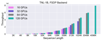
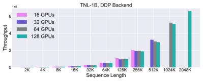
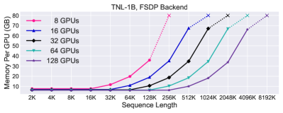
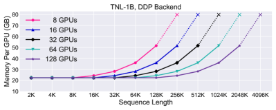
Figure 3: Scalability Evaluation of LASP on Throughput (tokens/sec) and Memory Usage. Left: Integration of LASP with FSDP backend; Right: Integration of LASP with DDP backend. The TNL-1B model is used, with a batch size of 1 across up to 128 A100 80GB GPUs. The sign "$\times$" with a dotted line represents occurring an Out of Memory (OOM).

4 Experiments

We evaluate LASP on two representative linear attention-based models: TransNormerLLM (TNL) (Qin et al., 2024a) and Linear Transformer (Katharopoulos et al., 2020). TNL is the latest large language model purely built upon linear attention, while Linear Transformer is a classical linear transformer model recognized in the community. Our assessment focuses on three key areas: I) the ability of LASP to scale up sequence length on scaling-out GPUs, II) the convergence when using LASP, and III) speed evaluation when using LASP and its comparison with other SP methods. No Activation Checkpointing (AC)  (Korthikanti et al., 2022) techniques are used in following experiments to reduce activation memory, except experiments in Section 4.3. This is because although the adoption of AC will further enables longer sequence lengths, it will cover up the ability of our sequence parallel method LASP. All experiments are conducted on a GPU cluster equipped with 128 A100 80G GPUs. Our implementation is built on MetaSeq (Zhang et al., 2022), a PyTorch-based sequence modeling framework with FairScale (FairScale authors, 2021) integrated. For more details of hardware and software, see Appendix A.1.

Experimental Setup.

The training configuration is set with specific hyperparameters: a learning rate of 0.0005 to control the step size, a cap of 50,000 updates to define the training duration, and a 2,000-update warmup period to stabilize early training by gradually adjusting the learning rate (Zhou et al., 2020). Additionally, a weight decay rate of 0.01 is used for regularization to avoid over-fitting. The Adam optimizer, with beta values of 0.9 and 0.999, is chosen for managing the momentum and scaling of gradients, aiding in effective and stable training convergence. Different DDP backends, including PyTorch DDP (abbr. DDP), Legacy DDP, FSDP, ZeRO-series, are selected in experiments for cross-validation of compatibility with LASP.

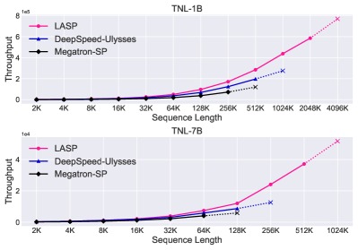
Figure 4: Speed Comparison (tokens/sec) of LASP Against DeepSpeed-Ulysses and Megatron-SP. The sign "$\times$" with a dotted line represents occurring an Out of Memory (OOM). The evaluation utilizes the TNL-1B and 7B models with a batch size of 1 on 64 A100 80GB GPUs. The parallelism size for these three methods is configured to 64.

4.1 Scalability and Speed Comparison

The scalability results regarding throughput and memory usage with varying sequence lengths and number of GPUs are illustrated in Fig. 3. By using LASP, we successfully scale the sequence length up to 4096K using the FSDP backend and 2048K with the DDP backend on a TNL model with 1B parameters, on 128 GPUs.

Importantly, the implementation of LASP allows for a linear increase in the maximum sequence length capacity, directly proportional (linear) to the number of GPUs used. For instance, a sequence length of 512K can be trained using 16 GPUs, while 64 GPUs ($4\times$) has is able to train 2048K ($4\times$) sequence length. Enabling LASP maintains a high throughput level even with more GPUs used. Furthermore, LASP demonstrates consistent scalability performance under both the FSDP and DDP backends. For more quantitative scalability results of LASP, see Table 4 in Appendix A.2.

Table 2: Convergence Performance of LASP. All experiments use 8 A100 80G GPUs, 16K sequence length, and batch size of 1. The results cover various DDP backends in conjunction with LASP. We explore the performance of two linear attention models: TransNormerLLM (TNL) and Linear Transformer, both with 0.4B parameters, across 50K updates.

Model	Parameters	Method	Loss	Method	Loss
TNL  (Qin et al., 2024a)	0 .4B	DDP	3.719	LASP + DDP	3.715
		Legacy DDP	3.709	LASP + Legacy DDP	3.705
		FSDP	3.717	LASP + FSDP	3.714
		ZeRO-1	3.653	LASP + ZeRO-1	3.653
		ZeRO-2	3.655	LASP + ZeRO-2	3.649
		ZeRO-3	3.656	LASP + ZeRO-3	3.649
Linear Transformer  (Katharopoulos et al., 2020)	0 .4B	DDP	5.419	LASP + DDP	5.408
		Legacy DDP	5.425	LASP + Legacy DDP	5.413
		FSDP	5.428	LASP + FSDP	5.441
		ZeRO-1	5.114	LASP + ZeRO-1	5.118
		ZeRO-2	5.105	LASP + ZeRO-2	5.120
		ZeRO-3	5.110	LASP + ZeRO-3	5.123

We furthermore conducted a comparison of sequence parallelism on TNL 1B and 7B models against two existing SP methods: DeepSpeed-Ulysses (Jacobs et al., 2023) and Megatron-SP (Korthikanti et al., 2022). All results presented in Fig. 4 are obtained on 64 GPUs. We keep using a fixed batch size of 1, in order to highlight the ability of LASP to handle extremely lone sequences.

LASP demonstrates a notable enhancement in throughput for linear attention, primarily due to its efficient communication design that facilitates the exchange of linear attention intermediate states. Specifically, LASP outperforms DeepSpeed-Ulysses by $38\%$ and Megatron by $136\%$ in terms of throughput at 256K sequence length on 1B model, with the performance gap widening as the sequence length increases. Additionally, system optimizations like kernel fusion and KV State caching enable LASP to support the longest sequence lengths within the same cluster, achieving 2048K for the 1B model and 512K for the 7B model.

4.2 Convergence

Table 2 presents convergence results of two linear-attention based models: TNL and Linear Transformer, evaluated on an epoch-by-epoch basis. The experiments were conducted using the same training corpus: the Pile (Gao et al., 2020). Both linear models has 0.4B parameters, demonstrated consistent loss values when training with or without LASP. All experiments undergoes 50K steps. The uniform loss convergence across various DDP backends demonstrates that LASP does not negatively affect model convergence.

4.3 Ablation on Activation Reducing Methods

LASP prominently reduces the activation memory usage during training process on per GPU, which is orthometric with another activation memory reducing method: activation checkpointing. Following we conduct ablation experiments on AC and LASP to reveal their performance on memory reduction. With pure DDP and FSDP, the maximum sequence lengths are able to train on 8 GPUs are 12K and 16K, respectively. Both AC and LASP can enlarge the maximum sequence length markedly, but encounters slightly throughput reduction. The distinction is the scaling-up performance of LASP is directly proportional to the number of GPUs used. By combining AC and LASP, we can obtain surprising maximum sequence lengths 496K and 768K on single node with using DDP and FSDP backends, respectively.

Table 3: Ablation on Activation Reducing Methods. Both DDP and FSDP backends are tested. A single node equipped with 8 A100 80G GPUs is used to train a TNL-1B model, still with a batch size of 1 for all experiments.

Method	Maximum Sequence Length	Throughput (tokens/sec)
DDP	12K	131286.0
DDP+AC	64K	117429.5
DDP+LASP	96K	126829.4
DDP+AC+LASP	496K	100837.8
FSDP	16K	145303.6
FSDP+AC	96K	114464.0
FSDP+LASP	120K	138598.8
FSDP+AC+LASP	768K	106578.3

5 Conclusion

We presented LASP, effectively addressing the limitations of existing SP methods on linear transformers by leveraging the specific features of linear attention, which significantly enhanced parallelism efficiency and usability for linear attention-based language models. Through the implementation of an efficient P2P communication mechanism and engineering optimizations such as kernel fusion and KV state caching, LASP achieved a notable reduction in communication traffic and improved hardware utilization on GPU clusters. Compatibility with all types of batch-level DDP methods ensured the practicability of LASP for large-scale distributed training. Our experiments highlighted the advantages of LASP on scalability, speed, memory usage and convergence performance for linear transformers, comparing with existing SP methods in out-of-box frameworks.

Broader Impact

This work presents a significant advancement in the field of artificial intelligence and machine learning, particularly in enhancing the efficiency and scalability of linear attention-based language models. By enabling the processing of sequences up to significantly longer than current methods and accelerating computational speed, LASP has the potential to vastly improve the performance in natural language understanding, genomic sequence analysis, time-series forecasting, and more. However, the increased capability and efficiency may also raise ethical and societal concerns, such as potential misuse in creating persuasive but misleading information, or in surveillance technology. Despite these concerns, the contributions of LASP on reducing computational costs and energy consumption in training large models could have positive environmental implications.

Appendix A Appendix

A.1 Hardware and Software

Hardware.

Our experimental configuration involves a maximum of 16 DGX-A100 servers, each equipped with 8 A100 GPUs, these GPUs are interconnected through NVSwitch, ensuring an inter-GPU bandwidth of 600GBps. For inter-node communication, we employ RoCE (RDMA over Converged Ethernet) technology, utilizing 8 RoCE RDMA adapters in each server. This setup facilitates efficient inter-server communication with a bandwidth capacity of 800Gbps.

Software.

Experiments are implemented in PyTorch 2.1.1 and Triton 2.0.0 with CUDA 11.7, cuDNN 8.0, and NCCL 2.14.3. Our algorithm is developed upon Metaseq 0.0.1. The Linear Transformer experiments build on https://github.com/idiap/fast-transformers.

A.2 Additional Experiment Results

See Table 4 in next page.

Table 4: Quantitative Scalability Results of LASP on Throughput (tokens/sec) and Memory Usage Per GPU (GB). Experiments are performed on TNL-1B, scaling sequence length from 2K to 4096K with a batch size of 1. Both DDP and FSDP backends are tested.

Sequence Length	GPUs	LASP + DDP		LASP + FSDP
		Throughput	Memory	Throughput	Memory
2K	16	1893.3	22.5	1780.5	6.9
	32	1645.4	22.5	1671.2	6.6
	64	1639.7	22.5	1589.8	6.4
	128	1610.9	22.5	1566.2	6.2
4K	16	3686.9	22.5	3519.9	6.9
	32	3458.4	22.5	3304.4	6.6
	64	3245.3	22.5	3152.2	6.4
	128	3211.5	22.5	3075.7	6.2
8K	16	7076.9	22.5	6924.8	6.9
	32	7319.3	22.5	6472.9	6.6
	64	6869.1	22.5	6459.4	6.4
	128	6793.6	22.5	6398.4	6.2
16K	16	14036.8	22.5	13513.7	6.9
	32	14671.7	22.5	12978.9	6.6
	64	13828.6	22.5	12569.4	6.4
	128	13484.5	22.5	12184.5	6.2
32K	16	28354.6	24.4	25727.2	6.9
	32	27863.6	22.5	26646.4	6.6
	64	25275.9	22.5	25201.4	6.4
	128	24523.8	22.5	25638.9	6.2
64K	16	52993.1	28.3	48542.8	11
	32	53393.2	24.4	49648.6	6.6
	64	52024.2	22.5	49780.5	6.4
	128	51983.3	22.5	49833.3	6.2
128K	16	107682	36.1	84901.9	19
	32	93371.5	28.3	92718.8	10.6
	64	100046	24.4	96771.6	6.4
	128	95828.5	22.5	98975.9	6.2
256K	16	202057	51.7	136765	35.2
	32	190675	36.1	159326	18.7
	64	193341	28.3	170996	10.4
	128	187347.7	24.4	178628.4	6.3
512K	16	OOM	OOM	201791	67.5
	32	323596	51.7	250663	34.8
	64	304366	36.1	284803	18.5
	128	295128.5	28.3	298755	10.1
1024K	16	OOM	OOM	OOM	OOM
	32	OOM	OOM	358478	67.1
	64	523119	51.7	437728	34.6
	128	508383	36.1	459794	18.2
2048K	16	OOM	OOM	OOM	OOM
	32	OOM	OOM	OOM	OOM
	64	OOM	OOM	585326	66.9
	128	658432	51.7	597953	33.8
4096K	16	OOM	OOM	OOM	OOM
	32	OOM	OOM	OOM	OOM
	64	OOM	OOM	OOM	OOM
	128	OOM	OOM	792705	66.2

References

- Choromanski et al. (2020) Choromanski, K., Likhosherstov, V., Dohan, D., Song, X., Gane, A., Sarlós, T., Hawkins, P., Davis, J., Mohiuddin, A., Kaiser, L., Belanger, D., Colwell, L. J., and Weller, A. Rethinking attention with performers. ArXiv, abs/2009.14794, 2020.
- Dao (2023) Dao, T. FlashAttention-2: Faster attention with better parallelism and work partitioning. arXiv preprint arXiv:2307.08691, 2023.
- Dao et al. (2022) Dao, T., Fu, D. Y., Ermon, S., Rudra, A., and Ré, C. FlashAttention: Fast and memory-efficient exact attention with IO-awareness. In Advances in Neural Information Processing Systems, 2022.
- FairScale authors (2021) FairScale authors. Fairscale: A general purpose modular pytorch library for high performance and large scale training. https://github.com/facebookresearch/fairscale, 2021.
- Gao et al. (2020) Gao, L., Biderman, S., Black, S., Golding, L., Hoppe, T., Foster, C., Phang, J., He, H., Thite, A., Nabeshima, N., Presser, S., and Leahy, C. The Pile: An 800gb dataset of diverse text for language modeling, 2020.
- Jacobs et al. (2023) Jacobs, S. A., Tanaka, M., Zhang, C., Zhang, M., Song, S. L., Rajbhandari, S., and He, Y. Deepspeed Ulysses: System optimizations for enabling training of extreme long sequence transformer models, 2023.
- Katharopoulos et al. (2020) Katharopoulos, A., Vyas, A., Pappas, N., and Fleuret, F. Transformers are RNNs: Fast autoregressive transformers with linear attention. In International Conference on Machine Learning, pp. 5156–5165. PMLR, 2020.
- Korthikanti et al. (2022) Korthikanti, V., Casper, J., Lym, S., McAfee, L., Andersch, M., Shoeybi, M., and Catanzaro, B. Reducing activation recomputation in large transformer models, 2022.
- Kwon et al. (2023) Kwon, W., Li, Z., Zhuang, S., Sheng, Y., Zheng, L., Yu, C. H., Gonzalez, J. E., Zhang, H., and Stoica, I. Efficient memory management for large language model serving with pagedattention, 2023.
- Lan et al. (2020) Lan, Z., Chen, M., Goodman, S., Gimpel, K., Sharma, P., and Soricut, R. ALBERT: A lite BERT for self-supervised learning of language representations, 2020.
- Li et al. (2023) Li, D., Shao, R., Xie, A., Xing, E. P., Gonzalez, J. E., Stoica, I., Ma, X., and Zhang, H. LightSeq: Sequence level parallelism for distributed training of long context transformers, 2023.
- Li et al. (2020) Li, S., Zhao, Y., Varma, R., Salpekar, O., Noordhuis, P., Li, T., Paszke, A., Smith, J., Vaughan, B., Damania, P., and Chintala, S. Pytorch Distributed: Experiences on accelerating data parallel training, 2020.
- Li et al. (2022) Li, S., Xue, F., Baranwal, C., Li, Y., and You, Y. Sequence Parallelism: Long sequence training from system perspective, 2022.
- Liu et al. (2023) Liu, H., Zaharia, M., and Abbeel, P. Ring attention with blockwise transformers for near-infinite context, 2023.
- Peng et al. (2021) Peng, H., Pappas, N., Yogatama, D., Schwartz, R., Smith, N. A., and Kong, L. Random feature attention. In 9th International Conference on Learning Representations, ICLR 2021, Virtual Event, Austria, May 3-7, 2021. OpenReview.net, 2021. URL https://openreview.net/forum?id=QtTKTdVrFBB.
- Qin & Zhong (2023) Qin, Z. and Zhong, Y. Accelerating toeplitz neural network with constant-time inference complexity. In Proceedings of the 2023 Conference on Empirical Methods in Natural Language Processing. Association for Computational Linguistics, December 2023.
- Qin et al. (2022a) Qin, Z., Han, X., Sun, W., Li, D., Kong, L., Barnes, N., and Zhong, Y. The devil in linear transformer. In Proceedings of the 2022 Conference on Empirical Methods in Natural Language Processing, pp. 7025–7041, Abu Dhabi, United Arab Emirates, December 2022a. Association for Computational Linguistics. URL https://aclanthology.org/2022.emnlp-main.473.
- Qin et al. (2022b) Qin, Z., Sun, W., Deng, H., Li, D., Wei, Y., Lv, B., Yan, J., Kong, L., and Zhong, Y. cosFormer: Rethinking softmax in attention. In International Conference on Learning Representations, 2022b. URL https://openreview.net/forum?id=Bl8CQrx2Up4.
- Qin et al. (2023a) Qin, Z., Li, D., Sun, W., Sun, W., Shen, X., Han, X., Wei, Y., Lv, B., Yuan, F., Luo, X., et al. Scaling transnormer to 175 billion parameters. arXiv preprint arXiv:2307.14995, 2023a.
- Qin et al. (2023b) Qin, Z., Sun, W., Lu, K., Deng, H., Li, D., Han, X., Dai, Y., Kong, L., and Zhong, Y. Linearized relative positional encoding. Transactions on Machine Learning Research, 2023b.
- Qin et al. (2024a) Qin, Z., Li, D., Sun, W., Sun, W., Shen, X., Han, X., Wei, Y., Lv, B., Luo, X., Qiao, Y., and Zhong, Y. TransNormerLLM: A faster and better large language model with improved transnormer, 2024a.
- Qin et al. (2024b) Qin, Z., Sun, W., Li, D., Shen, X., Sun, W., and Zhong, Y. Lightning Attention-2: A free lunch for handling unlimited sequence lengths in large language models, 2024b.
- Qin et al. (2024c) Qin, Z., Yang, S., and Zhong, Y. Hierarchically gated recurrent neural network for sequence modeling. Advances in Neural Information Processing Systems, 36, 2024c.
- Rabe & Staats (2021) Rabe, M. N. and Staats, C. Self-attention does not need memory. CoRR, abs/2112.05682, 2021. URL https://arxiv.org/abs/2112.05682.
- Rajbhandari et al. (2020) Rajbhandari, S., Rasley, J., Ruwase, O., and He, Y. Zero: Memory optimizations toward training trillion parameter models, 2020.
- Shoeybi et al. (2019) Shoeybi, M., Patwary, M., Puri, R., LeGresley, P., Casper, J., and Catanzaro, B. Megatron-LM: Training multi-billion parameter language models using model parallelism. arXiv preprint arXiv:1909.08053, 2019.
- Sun et al. (2024) Sun, W., Qin, Z., Sun, W., Li, S., Li, D., Shen, X., Qiao, Y., and Zhong, Y. CO2: Efficient distributed training with full communication-computation overlap. arXiv preprint arXiv:2401.16265, 2024.
- Tang et al. (2024) Tang, X., Sun, W., Hu, S., Sun, Y., and Guo, Y. MS-Net: A multi-path sparse model for motion prediction in multi-scenes. IEEE Robotics and Automation Letters, 9(1):891–898, 2024. doi: 10.1109/LRA.2023.3338414.
- Thakur et al. (2005) Thakur, R., Rabenseifner, R., and Gropp, W. Optimization of collective communication operations in mpich. The International Journal of High Performance Computing Applications, 19(1):49–66, 2005.
- Touvron et al. (2023a) Touvron, H., Lavril, T., Izacard, G., Martinet, X., Lachaux, M.-A., Lacroix, T., Rozière, B., Goyal, N., Hambro, E., Azhar, F., Rodriguez, A., Joulin, A., Grave, E., and Lample, G. LLaMA: Open and efficient foundation language models. arXiv preprint arXiv:2302.13971, 2023a.
- Touvron et al. (2023b) Touvron, H., Martin, L., Stone, K., Albert, P., Almahairi, A., Babaei, Y., Bashlykov, N., Batra, S., Bhargava, P., Bhosale, S., Bikel, D., Blecher, L., Ferrer, C. C., Chen, M., Cucurull, G., Esiobu, D., Fernandes, J., Fu, J., Fu, W., Fuller, B., Gao, C., Goswami, V., Goyal, N., Hartshorn, A., Hosseini, S., Hou, R., Inan, H., Kardas, M., Kerkez, V., Khabsa, M., Kloumann, I., Korenev, A., Koura, P. S., Lachaux, M.-A., Lavril, T., Lee, J., Liskovich, D., Lu, Y., Mao, Y., Martinet, X., Mihaylov, T., Mishra, P., Molybog, I., Nie, Y., Poulton, A., Reizenstein, J., Rungta, R., Saladi, K., Schelten, A., Silva, R., Smith, E. M., Subramanian, R., Tan, X. E., Tang, B., Taylor, R., Williams, A., Kuan, J. X., Xu, P., Yan, Z., Zarov, I., Zhang, Y., Fan, A., Kambadur, M., Narang, S., Rodriguez, A., Stojnic, R., Edunov, S., and Scialom, T. Llama 2: Open foundation and fine-tuned chat models, 2023b.
- Vaswani et al. (2017) Vaswani, A., Shazeer, N., Parmar, N., Uszkoreit, J., Jones, L., Gomez, A. N., Kaiser, Ł., and Polosukhin, I. Attention is all you need. Advances in neural information processing systems, 30, 2017.
- Yang et al. (2023) Yang, S., Wang, B., Shen, Y., Panda, R., and Kim, Y. Gated linear attention transformers with hardware-efficient training. arXiv preprint arXiv:2312.06635, 2023.
- Zhang et al. (2022) Zhang, S., Roller, S., Goyal, N., Artetxe, M., Chen, M., Chen, S., Dewan, C., Diab, M., Li, X., Lin, X. V., Mihaylov, T., Ott, M., Shleifer, S., Shuster, K., Simig, D., Koura, P. S., Sridhar, A., Wang, T., and Zettlemoyer, L. OPT: Open pre-trained transformer language models, 2022.
- Zhao et al. (2023) Zhao, Y., Gu, A., Varma, R., Luo, L., Huang, C.-C., Xu, M., Wright, L., Shojanazeri, H., Ott, M., Shleifer, S., et al. Pytorch FSDP: experiences on scaling fully sharded data parallel. arXiv preprint arXiv:2304.11277, 2023.
- Zheng et al. (2022) Zheng, L., Wang, C., and Kong, L. Linear complexity randomized self-attention mechanism. In International Conference on Machine Learning, pp. 27011–27041. PMLR, 2022.
- Zheng et al. (2023) Zheng, L., Yuan, J., Wang, C., and Kong, L. Efficient attention via control variates. In International Conference on Learning Representations, 2023. URL https://openreview.net/forum?id=G-uNfHKrj46.
- Zhou et al. (2020) Zhou, B., Liu, J., Sun, W., Chen, R., Tomlin, C. J., and Yuan, Y. pbSGD: Powered stochastic gradient descent methods for accelerated non-convex optimization. In IJCAI, pp. 3258–3266, 2020.