Planck dust polarization power spectra are consistent with strongly supersonic turbulence

Abstract

The polarization of the Cosmic Microwave Background (CMB) is rich in information but obscured by foreground emission from the Milky Way’s interstellar medium (ISM). To uncover relationships between the underlying turbulent ISM and the foreground power spectra, we simulated a suite of driven, magnetized, turbulent models of the ISM, varying the fluid properties via the sonic Mach number, $\mathcal{M_{S}}$, and magnetic (Alfvén) Mach number, $\mathcal{M_{\rm{A}}}$. We measure the power spectra of density ($\rho$), velocity ($v$), magnetic field ($H$), total projected intensity ($T$), parity-even polarization ($E$), and parity-odd polarization ($B$). We find that the slopes of all six quantities increase with $\mathcal{M_{S}}$ and tend to increase with $\mathcal{M_{\rm{A}}}$. By comparing spectral slopes of $E$ and $B$ to those measured by Planck, we infer typical values of $\mathcal{M_{S}}$ and $\mathcal{M_{\rm{A}}}$ for the ISM. As the fluid velocity increases, the ratio of BB power to EE power increases to approach a constant value near the Planck-observed value of $\sim 0.5$ for $\mathcal{M_{S}}>4$, regardless of the magnetic field strength. We also examine correlation-coefficients between projected quantities, and find that $r^{\rm{TE}}\approx 0.3$, in agreement with Planck, for appropriate combinations of $\mathcal{M_{S}}$ and $\mathcal{M_{\rm{A}}}$. Finally, we consider parity-violating correlations $r^{\rm{TB}}$ and $r^{\rm{EB}}$.

1 Introduction

Primordial gravitational waves, generated in inflation and imprinted on the surface of last scattering, are one of the most exciting sources of polarization in the Cosmic Microwave Background (CMB). Their discovery would give revolutionary evidence for inflation and its mechanism (Kamionkowski & Kovetz, 2016). However, the brightest diffuse sources of polarization in the microwave sky are thermal dust and synchrotron emission. These are also exciting signals, because they reveal the turbulent magnetic field in the interstellar medium (ISM) of our own Galaxy (Kritsuk et al., 2018; Kim et al., 2019). In order to see the potential inflation signal, we must first characterize and mitigate the Galactic signal which is at least ten times larger (Planck Collaboration et al., 2020).

Linearly polarized light can be described by the Stokes $Q,U$ parameters, which characterize the propagation of polarized light, but these quantities are coordinate dependent. The coordinate-independent $E,B$ parameters, on the other hand, convert the $Q,U$ signal into parity-even $E$ modes and parity-odd $B$ modes. At the surface of last scattering, cosmological scalar density perturbations produce $E$, while in the filamentary ISM, the $E$ modes are strongest for polarization parallel or perpendicular to a filament or sheet. On the other hand, at the surface of last scattering, gravitational waves (cosmological tensor perturbations) are the only producer of primordial $B$-mode polarization, peaking at degree scales and larger, while in the ISM, the $B$-modes are strongest for polarization at an oblique angle to a filament (Huffenberger et al., 2020). As the CMB signal travels from the surface of last scattering along the line of sight, gravitational lensing by large scale structure also generates $B$-modes, and CMB-lensing reconstruction could also be contaminated by ISM signals.

The Planck satellite measured $E$-mode and $B$-mode power spectra at 353 GHz, where the signal is dominated by dust emission, and found approximate powerlaws with slopes of $\alpha_{EE}=-2.42\pm 0.02$ and $\alpha_{BB}=-2.54\pm 0.02$ for a 71% sky area (Planck Collaboration et al., 2020). For the same sky area, the ratio of amplitudes of $B$ power to $E$ power was $0.53\pm 0.01$. They also found that the scalar temperature $T$-mode and $E$-mode are correlated with correlation coefficient $r^{TE}=0.36$ with some scatter but no clear trend with sky region or with angular scale. Curiously, the $T$-modes and $B$-modes are correlated with $r^{TB}=0.05$. This was unexpected as the correlation of a parity-even $T$-mode and a parity-odd $B$-mode should be zero on average in systems with no helicity or parity violation, and may indicate something about the structure of the magnetic field in the solar neighborhood (Planck Collaboration et al., 2020). Huffenberger et al. (2020) pointed out that in a filamentary picture, a positive $TB$ dust correlation would imply a positive $EB$ correlation, one that is too small to detect with Planck data alone, but is amenable to searches assisted with ISM tracers like HI (Cukierman et al., 2023).

In addition to searches for inflation, the polarization of the CMB can be used to hunt for signatures of other beyond-the-standard-model physics. Cosmic birefringence is the rotation of the polarization vector of CMB photons by hypothetical pseudoscalar fields. Possibilities include axion-like particles that may be responsible for dark matter (Komatsu, 2022). Minami & Komatsu (2020a) report the measurement of a rotation angle of $\beta=(0.35\pm 0.14)^{\circ}$ due to cosmic birefringence. In their work, they assume that the $E$ and $B$ polarization produced by the ISM are uncorrelated in order to set the calibration for the polarization angle. Because the sign of their correlation is the opposite of what is implied for dust in the filament picture, a nonzero $EB$ correlation in the dust would make their result stronger. (Minami & Komatsu, 2020b; Diego-Palazuelos et al., 2022, 2023, provide refinements and robustness tests.)

Simulations of the ISM (Kritsuk et al., 2018; Kim et al., 2019) and theoretical considerations (Caldwell et al., 2017; Kandel et al., 2017) have shown that for certain parameters, magnetohydrodynamic (MHD) turbulence can reproduce the expected $E$- and $B$-mode power spectra. That turbulence produces power-law polarization spectra is unsurprising, as $E$ and $B$ are produced by a combination of quantities that all have power law spectra due to the turbulent cascade: density (Beresnyak et al., 2005; Collins et al., 2012), velocity (Kolmogorov, 1941; Goldreich & Sridhar, 1995) and magnetic field (Grete et al., 2023).

In this work, we characterize how the polarization spectra depend on the MHD fluid parameters. We perform idealized simulations of MHD turbulence in order to characterize the $E$ and $B$ spectra and their correlations. We examine the power spectra of 3d fluid quantities, density $\rho$, velocity ${\bf v}$, and magnetic field ${\mathbf{H}}$; as well as 2d projected observable quantities, $T$, $E$, and $B$. From these results, we infer averaged properties of the ISM from the Planck measurements.

We organize our paper as follows. We describe the methods for simulations and analysis in Section 2. We present results, beginning with a short overview, in Section 3. There we show power spectra and slopes for both fluid (Section 3.1) and projected quantities (Section 3.2). We present ratios and correlation coefficients (Section 3.3). Using the measured quantities from Planck, we posit typical values for the ISM’s sonic and Alfvén Mach numbers (Section 3.5). We briefly contrast these findings with projections parallel to the mean magnetic field (Section 3.6). We conclude in Section 4.

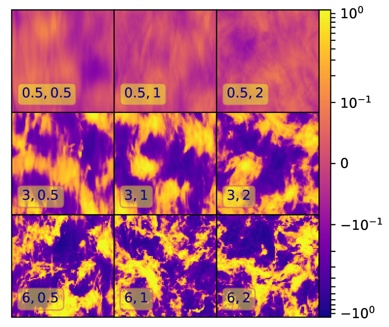
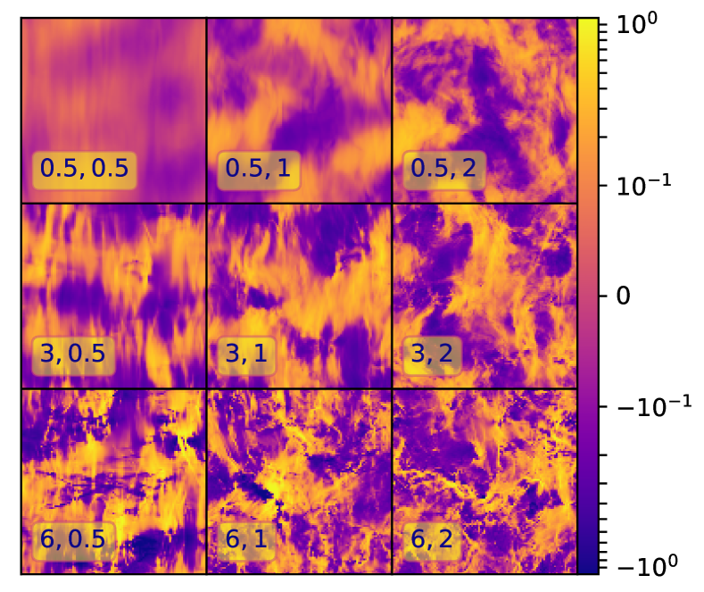
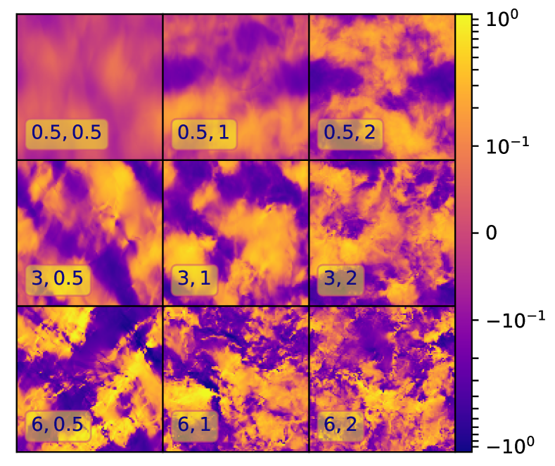
Figure 1: Images of $\ln(T)$ (top), $E$ (middle), and $B$ (bottom). The mean magnetic field points up. The colorbar is a symmetric logarithm. In each $3\times 3$ panel, simulations with weaker magnetic fields (higher $\mathcal{M_{\rm{A}}}$) are to the right and simulations with faster fluid flow (higher $\mathcal{M_{\rm{s}}}$) are to the bottom. Nine of the 21 total simulations are shown, with the targeted $(\mathcal{M_{\rm{s}}},\mathcal{M_{\rm{A}}})$ indicated in the box.

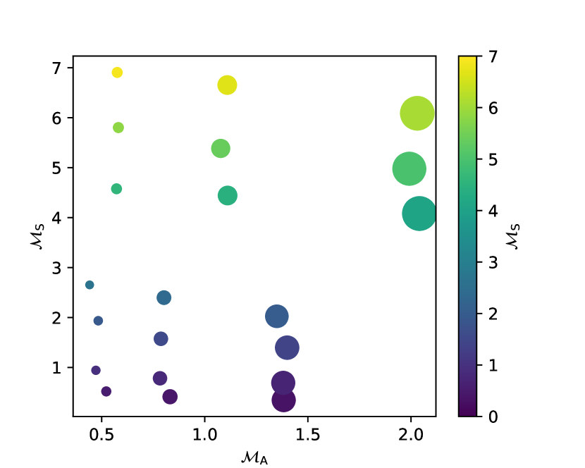
Figure 2: Legend of sonic and Alfén Mach numbers, $\mathcal{M_{S}}$ and $\mathcal{M_{\rm{A}}}$, for each simulation. As with all future plots, color denotes $\mathcal{M_{S}}$, with blue-to-yellow indicating indicating increasing sonic Mach numbers (and faster rms fluid velocity). Marker size denotes $\mathcal{M_{\rm{A}}}$ (increasing size indicates increasing $\mathcal{M_{\rm{A}}}$, and weaker influence of the magnetic field),

2 Methods

We perform a suite of idealized simulations of the intersteller medium. From the 3d simulation boxes, we compute temperature and polarization images, and then compute spectra of 3d and 2d physical quantities. Ideal MHD has three independant quantities: density, $\rho$, velocity, ${\bf v}$, and magnetic field, ${\mathbf{H}}$. With the ansatz that turbulence dictates the primary behavior in $E$- and $B$-modes, we examine the variation in power spectra in all six quantities of interest: the three fluid quantities, $\rho$, ${\bf v}$, and ${\mathbf{H}}$; and the three projected quantities, $T$, $E$, and $B$.

2.1 Simulations

The simulations utilize the open source code Enzo (Wang & Abel, 2009; Bryan et al., 2014) to solve the Eulerian equations of ideal magnetohydrodynamics (MHD). We used the Dedner et al. (2002) divergence cleaning scheme with a piecewise linear reconstruction and HLLD Riemann solver (Mignone, 2007). With an adiabatic index $\gamma-1=10^{-3}$, we achieve a reasonable approximation to an isothermal equation of state.

The simulation boxes are periodic, use a $512^{3}$-zone resolution, and start with uniform density. To generate turbulence, we drive the fluid with a stochastic forcing that adds a random acceleration pattern

to the velocity field in a way that keeps the energy injection rate constant (Mac Low & Klessen, 2004; Federrath et al., 2010). The driving is applied for ten dynamical times, $t_{\rm{dyn}}=L_{0}/\mathcal{M_{S}}$, where $L_{0}=1/2$ is the pattern size and $\mathcal{M_{S}}$ is the r.m.s. velocity. The first 5$t_{\rm{dyn}}$ are ignored, and used only to establish the fully developed turbulence. The remaining 5$t_{\rm{dyn}}$ are used for analysis. The force is distributed as a Gaussian in each component, with power only on large spatial scales, $k/k_{\rm min}\in[1,2]$. The forcing pattern is evolved in time with an Ornstein-Uhlenbeck (OU) process (Federrath et al., 2010). This means that the driving pattern retains only 1/e of its correlation after $t_{\rm{dyn}}$. The input power is split between compressible and solenoidal modes such that the ratio of compressive to solenoidal amplitude is 2/3 ($\zeta$ = 1/2 in Equation 6 of Federrath et al. (2010)). It is anticipated in the inertial range for compressible turbulence, the natural ratio is 2/3 (Kritsuk et al., 2007). We have checked that the driving field’s helicity ($\int dV\ \mathbf{v}\cdot(\nabla\times\mathbf{v})$) is zero to machine precision, so we do not expect the driving to introduce parity violation.

Ideal isothermal MHD is scale free. The dynamics depend on only two parameters, and we choose the Sonic Mach number $\mathcal{M_{S}}$, and the Alfvén Mach number, $\mathcal{M_{\rm{A}}}$:

$$\mathcal{M_{S}} =v_{\rm rms}/c_{s}$$ (1)

$$\mathcal{M_{\rm{A}}} =v_{\rm rms}/v_{A}$$ (2)

$$v_{A} =H/\sqrt{4\pi\rho}$$ (3)

where $\rho$ is the mean density, $v_{A}$ is the Alfvén velocity, $c_{s}$ is the speed of sound, and $H$ is the mean magnetic field strength. Stronger field means bigger $v_{A}$ and thus smaller $\mathcal{M_{\rm{A}}}$.

Throughout the work we define $\mathcal{M_{S}}$ and $\mathcal{M_{\rm{A}}}$ with the 3D velocity dispersion, $v_{\rm rms}^{2}=\langle v_{x}^{2}\rangle+\langle v_{y}^{2}\rangle+\langle v_{z}^{2}\rangle$. In contrast to the 3D Mach number $\mathcal{M_{S}}$, the 1D Mach number (which enters the Maxwellian velocity distribution (Rabatin & Collins, 2023) and is more accessible from the ground) is found by assuming isotropy and dividing $v_{\rm rms}$ by $\sqrt{3}$.

To probe the parameter space, we target nominal sonic Mach numbers

$$\mathcal{M_{S}}=0.5,1,2,3,4,5,6$$

and nominal Alfven Mach numbers

$$\mathcal{M_{\rm{A}}}=0.5,1,2$$

across the suite of 21 simulations. The actual $\mathcal{M_{S}}$ and $\mathcal{M_{\rm{A}}}$ realized by the simulations differ slightly from these nominal values.

Figure 1 shows $\ln(T)$, $E$, and $B$ (defined precisely in the following section). Each figure shows three target Sonic Mach numbers, (0.5, 3, 6) and Alfvén Mach numbers (0.5, 1, 2). The colorbar is a symmetric logarithm. Clearly, structure changes as $\mathcal{M_{S}}$ and $\mathcal{M_{\rm{A}}}$ increase. This is due to the fact that the dissipation scale decreases as the mean kinetic energy increases.

Figure 2 shows a legend of the achieved $\mathcal{M_{S}}$ and $\mathcal{M_{\rm{A}}}$ for each simulation. Because it is challenging to predict the forcing to achieve particular Mach numbers, the measured values of $\mathcal{M_{S}}$ and $\mathcal{M_{\rm{A}}}$ differ slightly from the nominal values listed above. This figure also serves as a legend for the remaining figures in the work, with color denoting mach number, with dark blue-to-yellow corresponding to achieved $\mathcal{M_{S}}$, ranging from subsonic ($\mathcal{M_{S}}<1$) to supersonic ($\mathcal{M_{S}}\sim 7$).

Marker size increases with $\mathcal{M_{\rm{A}}}$, so larger markers denote weaker magnetic field strength. In the power-spectra plots, we will use linestyles to denote $\mathcal{M_{\rm{A}}}$, with dotted lines for $0.4<\mathcal{M_{\rm{A}}}<0.7$, dashed lines for $0.7<\mathcal{M_{\rm{A}}}<1.2$, and solid lines for $1.2<\mathcal{M_{\rm{A}}}<2.2$.

2.2 Projection to dust temperature and polarization

The polarization we are focusing on here comes from elongated dust grains that rotate around the local magnetic field, with their long axis perpendicular to the field direction. We make several simplifying assumptions: the dust-to-gas ratio is constant and uniform, the dust grains perfectly align with the magnetic field, the cloud is optically thin, the dust temperature is the same as the gas temperature (which are both constant and uniform), and there is only one dust species. The boxes are scale-free and do not correspond to any particular physical size.

We focus most of our attention on projections perpendicular to the mean magnetic field. This is because observations oblique to the mean magnetic field are more likely than along the mean magnetic field, as the solid angle for to vectors to be nearly aligned is much smaller than it is for them to be nearly perpendicular. Of course, line-of-sight alignment may exist over some portion of the sky, and the true picture is a mixture of angles. We will start with the more observable case, and return to discuss parallel projections in section 3.6.

From the assumption of optically thin dust, the $T$-mode is simply proportional to the column density,

$$T=\int\rho dz.$$ (4)

To compute $E$ and $B$, we first compute Stokes parameters $Q$ and $U$, which are closely related to the observable quantities. These are

$$Q =\int\rho\cos{2\psi}\cos^{2}{\gamma}dz$$ (5)

$$U =\int\rho\sin{2\psi}\cos^{2}{\gamma}dz,$$ (6)

where $\psi$ is the angle the field makes in the plane of the sky relative to horizontal, and $\gamma$ is the angle between the magnetic field and the plane of the sky (Bohren & Huffman, 1998; Fiege & Pudritz, 2000). For projections along the $\hat{z}$-axis line-of-sight, and choosing $\hat{x}$ as the horizontal direction, this gives

$$Q =\int\rho\frac{H_{y}^{2}-H_{x}^{2}}{H_{x}^{2}+H_{y}^{2}+H_{z}^{2}}dz$$ (7)

$$U =\int\rho\frac{H_{y}H_{x}}{H_{x}^{2}+H_{y}^{2}+H_{z}^{2}}dz.$$ (8)

In the flat-sky approximation, the coordinate-invariant quantities $E$ and $B$ are then found as

$$\tilde{E}+i\tilde{B} =\left(\tilde{Q}+i\tilde{U}\right)e^{-2i\theta_{k}},$$ (9)

where $\tilde{E}$ denotes the Fourier transform of $E$, and $\cos\theta_{k}={k_{x}}/{({k_{x}^{2}+k_{y}^{2}})^{1/2}}$ is the angle in Fourier space (Kamionkowski & Kovetz, 2016).

2.3 Power spectra

We compute the average power spectra of all quantities by averaging over a shell or annulus in Fourier space:

$$C_{k}^{XY}=\frac{1}{\Delta V_{k}}\int_{||{\bf k}^{\prime}|-k|<\Delta k}d^{D}{\bf k}^{\prime}\tilde{X}({\bf k}^{\prime})\tilde{Y}({\bf k}^{\prime})$$ (10)

where $\tilde{X}$ and $\tilde{Y}$ are Fourier transforms of fluid quantities ($\rho$, $\mathbf{v}$, and $\mathbf{H}$, whence dimension $D=3$) or projected quantities ($T$, $E$, and $B$, whence $D=2$). $\Delta V_{k}$ is the volume of a shell at $k$, which has thickness matched to the resolution of the Fourier grid, $\Delta k=k_{\rm min}=2\pi/L$. Because the box is scale-free, the wavenumbers $k$ do not correspond to any particular angular scale or multipole.

For vector quantities the product $XY$ is replaced with the vector dot product, e.g.

$$C_{k}^{vv}=C_{k}^{v_{x}v_{x}}+C_{k}^{v_{y}v_{y}}+C_{k}^{v_{z}v_{z}},$$ (11)

and a similar expression for the magnetic field.

Quite often the turbulence literature employs the contribution to the total power in a shell, which omits the shell volume, $\Delta V_{k}$, in Equation 10, while the cosmology literature uses the average power in the shell for the CMB and large-scale structure. The convention in the turbulence literature is due to the relationship between the power spectrum and the total energy in the system (e.g. Pope, 2000). The slope of total-power spectrum can be recovered from the average-power spectra presented here as $\alpha_{\rm{total}}=\alpha_{XX}+2$ in three-dimensions. This is most apparent when examining the velocity spectrum: the total power in the traditional Kolmogorov cascade is $\alpha_{\rm{total}}=-5/3$, while the average value is $-11/3$. We use the average spectrum throughout to connect with the Planck-measured CMB power spectra.

Each spectra can be broken into three regimes. At large scales ($k<k_{\rm{drive}}$), the driving of the turbulence dominates these spectra, which depends on the details of the simulator’s particular setup. At small scales ($k>k_{\rm{diss}}$), the spectra is dominated by numerical dissipation. In between, in the so-called inertial range where we are most interested in the behavior, the spectra are set by the nonlinear dynamics of the system. Empirically, we use $k_{\rm{drive}}=4k_{\rm{min}}$ and $k_{\rm{diss}}=25k_{\rm{min}}$, as this range captures the nearly-powerlaw section of each of the spectra (visible in Fig. 4 and Fig. 6). In this range, we fit the spectra to the form

$$C_{k}^{XX}=A_{\rm{XX}}k^{\alpha_{XX}}.$$ (12)

To estimate uncertainties on the spectral slopes, we computed $\alpha_{XX}$ for every simulation timestep, also varying $k_{\rm{drive}}\in[3,4,5]k_{\rm{min}}$ and $k_{\rm{diss}}\in[25,26,27,28]k_{\rm{min}}$, and took the standard deviation of the collection.

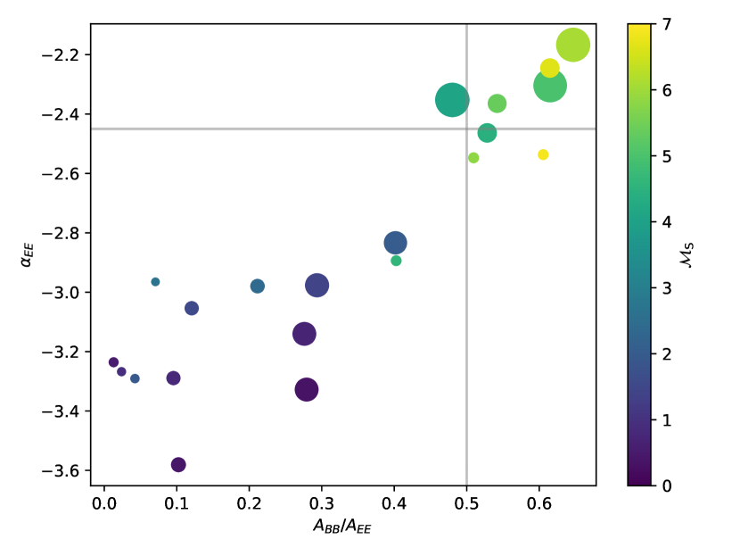
Figure 3: A summary of the slope of $E$-mode vs. the ratio of amplitudes, $A_{\rm{BB}}/A_{\rm{EE}}$. The grey lines denote the approximate values from Planck Collaboration et al. (2020): $\alpha_{EE}=-2.42$, $A_{\rm{BB}}/A_{\rm{EE}}=0.5$. Color and marker size are as described in Section 2.1

3 Results

Figure 3 gives an overview of the main result for foreground polarization. The vertical axis shows $\alpha_{EE}$ while the horizontal shows $A_{\rm{BB}}/A_{\rm{EE}}$ (the ratio of the fit amplitudes). Grey lines indicate the Planck-measured values. The color shows the Mach number $\mathcal{M_{S}}$ and the size shows $\mathcal{M_{\rm{A}}}$ (as in Fig. 2). As discussed below, as $\mathcal{M_{S}}$ increases above 4, the ratio $A_{\rm{BB}}/A_{\rm{EE}}$ increases to sit in the range [0.4,0.7], compared to the Planck value near 0.5, and $\alpha_{EE}$ becomes shallower to a range $[-2.6,-2.2]$, compared to the Planck value of -2.42.

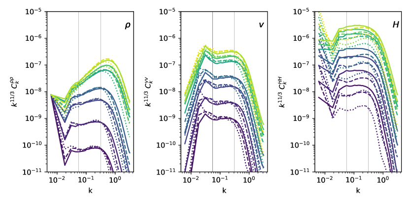
Figure 4: Power spectra of density ($C_{k}^{\rho\rho}$), velocity ($C_{k}^{vv}$) and magnetic field strength ($C_{k}^{HH}$) (left to right, respectively.) All plots have been compensated to the Kolmogorov value of 11/3. Color (blue-yellow) denotes increasing Mach number, while linestyle denotes $\mathcal{M_{\rm{A}}}$ as described in Section 2.1: dotted lines for $0.4<\mathcal{M_{\rm{A}}}<0.7$, dashed lines for $0.7<\mathcal{M_{\rm{A}}}<1.2$, and solid lines for $1.2<\mathcal{M_{\rm{A}}}<2.2$. Density slope depends heavily on Mach number, while velocity and magnetic slopes do not.

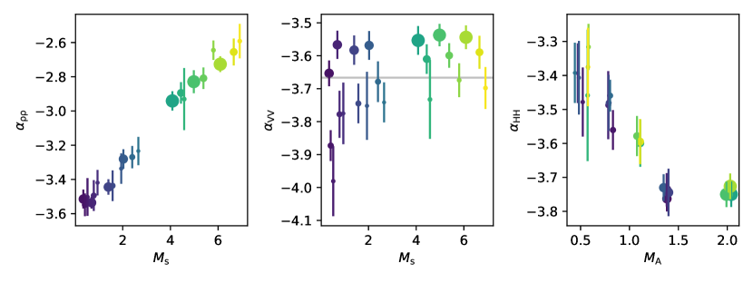
Figure 5: Slopes of fluid quantities ($\rho$, ${\bf v}$, and ${\mathbf{H}}$). The first column of each plot shows (slopes, amplitdues) relative to $\mathcal{M_{S}}$ for the first two, and $\mathcal{M_{\rm{A}}}$ for $\alpha_{HH}$. Color denotes $\mathcal{M_{S}}$ while size denotes $\mathcal{M_{\rm{A}}}$ as described in Section 2.1.

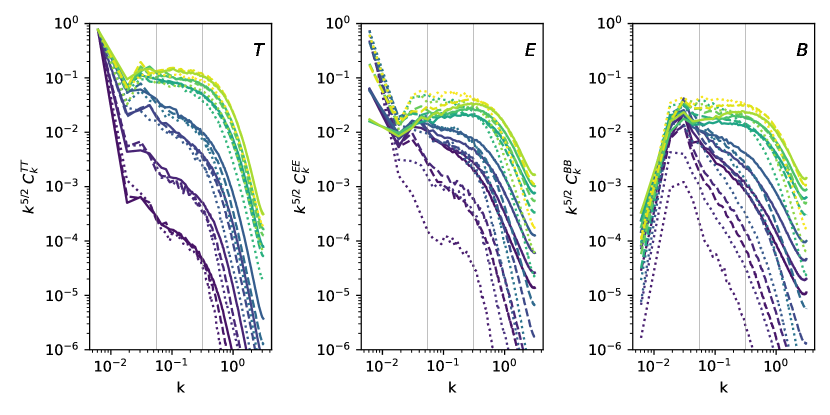
Figure 6: Spectra of projected quantities, $C_{k}^{TT}$, $C_{k}^{EE}$, and $C_{k}^{BB}$. Each spectra has been compensated to $k^{2.5}$ to emphasize the variation with simulation. Color denotes $\mathcal{M_{S}}$ and linestyle denoste $\mathcal{M_{\rm{A}}}$, as described in Section 2.1: dotted lines for $0.4<\mathcal{M_{\rm{A}}}<0.7$, dashed lines for $0.7<\mathcal{M_{\rm{A}}}<1.2$, and solid lines for $1.2<\mathcal{M_{\rm{A}}}<2.2$.

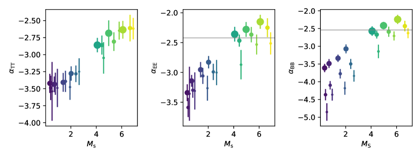
Figure 7: Slopes of intensity and polarization power spectra versus sonic Mach number. The horizontal axis and color denote $\mathcal{M_{S}}$ while size denotes $\mathcal{M_{\rm{A}}}$ as described in Section 2.1. Grey lines denote the values observed by Planck

3.1 Fluid Power Spectra

Figures 4 display the spectra for the fluid quantities, $C_{k}^{\rho\rho}$ (density, left), $C_{k}^{{vv}}$(velocity, center) and $C_{k}^{HH}$ (magnetic field, right). Figure 5 shows the slopes of those spectra, $\alpha_{\rho\rho}$ (left), $\alpha_{{vv}}$ (center) and $\alpha_{HH}$ (right). The spectra are compensated by $k^{11/3}$ to emphasize variations relative to the average Kolmogorov slope value, which would be flat in this plot. The plot style is described in Section 2.1; color (blue to yellow) denotes increasing $\mathcal{M_{S}}$, while line style denotes $\mathcal{M_{\rm{A}}}$. Figure 5 shows the slopes, $\alpha_{XX}$, with color denoting $\mathcal{M_{S}}$ and point size increasing with $\mathcal{M_{\rm{A}}}$.

Density

Beginning with density (first panels in Figures 4 and 5) we find that both slope and amplitude are increasing functions of $\mathcal{M_{S}}$. The increase in amplitude is to be expected, as the variance in density is linearly proportional to the variance in velocity (Federrath et al., 2008), i.e.

$$\sigma^{2}_{\rho}=b^{2}\sigma^{2}_{v},$$ (13)

where $b\in[1/3,1]$. By the Plancherel theorem $\sigma^{2}_{\rho}$ is an integral of the power spectrum, so it is expected that the amplitude of the density power spectra will increase with Mach number. The slope becomes shallower in an almost linear way from $\alpha_{\rho\rho}\sim-3.5$ to $\alpha_{\rho\rho}\sim-2.5$ as $\mathcal{M_{S}}$ increases from 0.5 to 7. As $\mathcal{M_{S}}$ increases, the typical shock velocity also increases, which gives rise to enhanced structure formation by way of fluid instabilities such as the Richtmyer-Meshkov instability (Richtmyer, 1960; Meshkov, 1972). This enhanced power flattens the spectrum. This behavior has been seen before (Beresnyak et al., 2005; Collins et al., 2012). Neither slope, $\alpha_{\rho\rho}$ nor amplitude, $A_{\rho}$ vary with Alfvén Mach number. This is not particularly surprising, as the continuity equation which determines density only contains density and velocity:

$$\frac{\partial\rho}{\partial t}+\nabla\cdot{\bf v}\rho=0,$$

so the density is determined by velocity. We see that the density power spectrum is apparently determined solely by way of the r.m.s. velocity.

Velocity

The velocity field (second panels of Figures 4 and 5) can be seen to vary jointly with $\mathcal{M_{\rm{A}}}$ and $\mathcal{M_{S}}$. In incompressible hydrodynamical turbulence, the expectation is that the slope has the (average) Kolmogorov value of $-11/3\approx-3.7$. These simulations are not imcompressible, but highly compressible and magnetized. For supersonic hydrodynamical turbulence, one expects a value of $\alpha_{{vv}}=-4$ or ($\alpha_{\rm{total}}=-2$, Kritsuk et al. 2007.) For incompressible magnetized turbulence, we expect a value of $\alpha_{v}=-5/2$ along the field, and $\alpha_{v}=-11/3$ transverse to the magnetic field ($\alpha_{\rm{total}}=-3/2$ and $-5/3$, respectively, Goldreich & Sridhar 1995). There is not a theory that combines compressibility and magnetization that is appropriate for the simulations presented here, and in our case we see some resemblance to all of the above. The simulation that most closely approaches the un-magnetized incompressible assumption of the Kolmogorov cascade has $\mathcal{M_{S}}$$=0.5$ and $\mathcal{M_{\rm{A}}}$$=2$, which does have a slope of $-3.6$. For low $\mathcal{M_{S}}$, the slope $\alpha_{{vv}}$ steepens from $-3.6$ to $-3.9$ as the field increases (dot size shrinks). Once supersonic, the slope of the velocity does not vary much with $\mathcal{M_{S}}$, but does steepen with increasing field strength. For low field strength, the slope is around around $\alpha_{{vv}}=-3.5$ ($\alpha_{\rm{total}}=-1.5$).

Magnetic field

The final fluid quantity is magnetic field, ${\mathbf{H}}$. Spectra are plotted in Figure 4, and slopes are plotted in Figure 5). Here the magnetic slope, $\alpha_{HH}$ is plotted against Alfvén Mach number rather than Sonic Mach number. It can be seen that the slope of the magnetic field, $\alpha_{HH}$, does not depend strongly on $\mathcal{M_{S}}$, as points with similar color cluster around the same value, but does decrease nearly linearly for decreasing magnetic field strength. For the weakly magnetized runs, $\alpha_{HH}=-3.75$, and it increases to $-3.3$ for the strongly magnetized runs. This is an intuitively reasonable result, as the magnetic field strength increases ($\mathcal{M_{\rm{A}}}$ decreases) the ability of the field to resist tangling by kinetic motions increases, which suppresses power at all scales, but especially large scales, making the slope more shallow.

3.2 Projected Intensity and Polarization Power Spectra

Figures 6 and 7 show the spectra and slopes for projected quantities, $T$, $E$ and $B$. Color denotes $\mathcal{M_{\rm{A}}}$ (blue-to-yellow denotes increasing $\mathcal{M_{S}}$) and line style denotes $\mathcal{M_{\rm{A}}}$ (solid, dashed, and dotted denoting increasing value) as described in Section 2.1. All projected spectra have been compensated so that slope of $\alpha=-2.5$ would appear flat and horizontal.

Intensity/Temperature

The $T$ spectrum, $C_{k}^{TT}$, can be seen in the first panel of Figures 6 and its slope, $\alpha_{TT}$, in the first panel of Figure 7. The $T$ spectrum has a slope that is nearly identical to the $\rho$ spectrum (though they appear different due to the difference in compensation). This is expected as in this model, $T$ is simply the projection of $\rho$. By the slice-projection theorem, given a quantity $q(x,y,z)$, its projection $Q(x,y)$, and their Fourier transforms $\hat{q}(k_{x},k_{y},k_{z})$ and $\hat{Q}(k_{x},k_{y})$ are related as

$$\hat{Q}(k_{x},k_{y})=\hat{q}(k_{x},k_{y},k_{z}=0).$$ (14)

That is, the transform of the projection is the zero mode of the transform along the projection axis. Thus one can reasonably expect $T$ and $\rho$ to have the same average power spectra, provided the field is isotropic. Thus, $T$ power spectral slopes and amplitudes should also depend primarily on $\mathcal{M_{S}}$ in the same linear fashion as $\alpha_{\rho}$. The match is not exact due to the fundamentally anisotropic nature of our simulations’ mean magnetic fields, but quite similar.

E-mode

The even-parity $E$ spectrum, $C_{k}^{EE}$, can be seen in the second panel of Figures 6 and its slope, $\alpha_{EE}$, in the second panel of Figure 7. The grey line in Figure 7 shows the observed value of -2.42. It can be seen that $\alpha_{EE}$ depends on $\mathcal{M_{S}}$ nearly linearly, and $\mathcal{M_{\rm{A}}}$ somewhat. As the sonic Mach number increases, we find that $\alpha_{EE}$ get shallower from $-3.5$ for $\mathcal{M_{S}}=0.5$ to $-2.3$ for $\mathcal{M_{S}}=6$. Increasing magnetic field (decreasing $\mathcal{M_{\rm{A}}}$) steepens the $\alpha_{EE}$ slope. Simulations with $\mathcal{M_{S}}\geq 4$ are needed to reproduce the measured Planck $\alpha_{EE}$. Simulations with gas velocities that are too slow yield slopes that are too steep. The amplitude of the $E$ power increases for decreasing field when $\mathcal{M_{S}}$ is low, but is relatively immune to both $\mathcal{M_{S}}$ and $\mathcal{M_{\rm{A}}}$ for supersonic runs.

B-mode

The odd-parity $B$ spectrum, $C_{k}^{BB}$, can be seen in the right panel of Figure 6, and its slope, $\alpha_{BB}$, can be seen in the right panel of Figure 7. The slope depends on $\mathcal{M_{S}}$ like $\alpha_{EE}$ but has a stronger dependence on $\mathcal{M_{\rm{A}}}$, particularly when $\mathcal{M_{\rm{A}}}$ is small (strong field). For the weakly magnetized runs, $\alpha_{BB}$ ranges from $-3.5$ to $-2.1$.

Compared to the the other projected slopes, there is a strong steepening of the slope $\alpha_{BB}$ at all $\mathcal{M_{S}}$ as $\mathcal{M_{\rm{A}}}$ decreases. That is, stronger magnetic fields result in steeper power spectra in the $B$ mode. We may interpret this reduction in power as a stiffening of the filamentary structure, which cause the field and filament to more likely align on small scales. We revisit this interpretation in the discussion.

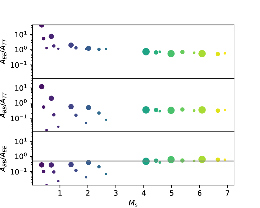
Figure 8: Ratios of amplitudes converge on (0.62, 0.34, 0.55) for $E/T$, $B/T$, and $B/E$, respectively. Colors are described in Section 2.1. A value of 0.5 is seen as the grey line in each row.

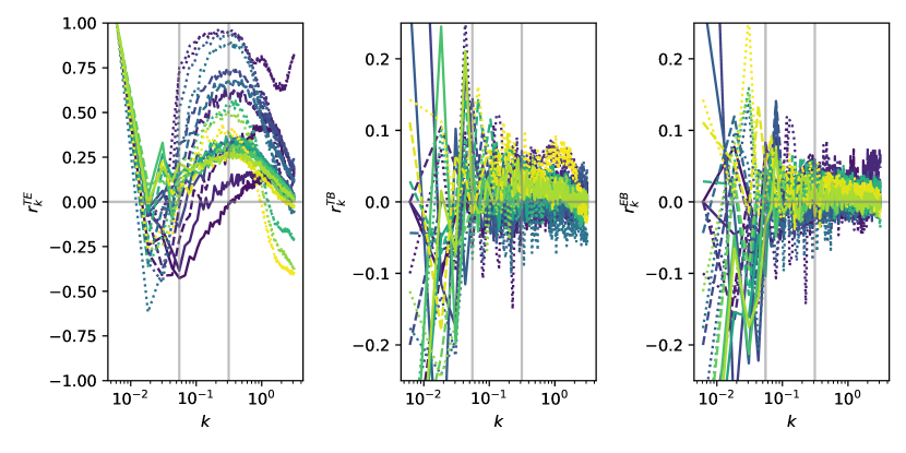
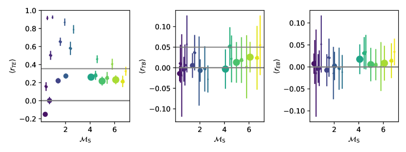
Figure 9: (Top) Correlation ratio $r_{xy}$ for TE, TB, and EB spectra. Vertical bars show the analysis window. (Bottom) Average $r_{XY}$ in the analysis window versus Sonic Mach number KMH: label missing, $\mathcal{M_{S}}$, compared to Planck-measured values. In the top plots, we use dotted lines for $0.4<\mathcal{M_{\rm{A}}}<0.7$ (smallest point size at bottom), dashed lines for $0.7<\mathcal{M_{\rm{A}}}<1.2$, and solid lines for $1.2<\mathcal{M_{\rm{A}}}<2.2$ (largest point size at bottom). See text for cautions about interpreting the $\langle r_{TB}\rangle$ and $\langle r_{TE}\rangle$.

3.3 Power Amplitude Ratios

The ratio of $B$ power to $E$ power is interest because the observed value of $A_{\rm{BB}}/A_{\rm{EE}}=0.53$ was unexpected. We can also examine the ratio of of $E$ and $B$ relative to total power, $A_{\rm{EE}}/A_{\rm{TT}}$ and $A_{\rm{BB}}/A_{\rm{TT}}$, though our model lacks a detailed treatment of the dust polarization fraction, which implies that these ratios cannot be directly compared to observed values, though the trend with $\mathcal{M_{S}}$ and $\mathcal{M_{\rm{A}}}$ can be measured. The polarization fraction cancels out in the $A_{\rm{BB}}/A_{\rm{EE}}$ ratio, so this can be directly compared to the Planck value.

Figure 8 shows the ratio of fit amplitudes, $A_{\rm{EE}}/A_{\rm{TT}}$, $A_{\rm{BB}}/A_{\rm{TT}}$, and $A_{\rm{BB}}/A_{\rm{EE}}$ versus the sonic Mach number in each of the three panels. The third panel also shows the observed value as a grey line. The runs with slower velocities show the most $E$ modes, as the low velocity causes the field to have larger impact on the morphology, and more filamentary structures that align magnetic field and density are observed. This can be seen in the projections in Figure 1. The runs with the slower velocities show the largest $B$ modes as well, when the Alvèn Mach number is large and the magnetic fields are weak. But when then the magnetic fields are strong, the slower velocities show the weakest B modes. For higher velocity Mach numbers ($\mathcal{M_{S}}\geq 4$), the amplitude ratios depend little on either the fluid velocity or the magnetic field. For $\mathcal{M_{S}}>4$, the ratio tends toward $A^{BB}/A^{EE}=0.55\pm 0.07$, near to the observed ratio of Planck. Thus it may be that that the ratio of $B$ to $E$ observed by Planck is a natural consequence of compressive turbulence, and that $A_{\rm{BB}}/A_{\rm{EE}}=0.53$ simply because the flow is hypersonic and magnetized, which naturally gives this value.

3.4 Cross-correlations

Figure 9 shows the correlation coefficient spectra,

$$r^{\rm{XY}}_{k}={C_{k}^{XY}}/{\sqrt{C_{k}^{XX}\times C_{k}^{YY}}},$$ (15)

for all pairs of $T$, $E$, and $B$. The top row shows the spectra, with the fitting window denoted by vertical light-grey lines. The bottom row shows $\langle r^{\rm{XY}}\rangle$, averaged over the fit window and all frames, as a function of Mach number. Error bars are found by first averaging $r_{k}^{XY}$ over $k$ for each frame within the fit window, then taking the variance over frames. Shown in horizontal grey lines are the observed values of $r^{\rm{TE}}=0.355$ and $r^{\rm{TB}}=0.055$ (Planck Collaboration et al., 2020).

For the two even-parity modes, $T$ and $E$, we find significant positive correlation in all cases but one. As the velocity decreaess and magnetic field increaes, $r^{\rm{TE}}$ increases well above the value observed by Planck. The general trend is of increasing correlation with increasing field strength. For large Mach numbers, correlations are more modest and mostly consistent with the observed Planck value of $r^{\rm{TE}}=0.35$. For large $\mathcal{M_{S}}$, the effect of the magnetic field is not as pronounced as it is for lower $\mathcal{M_{S}}$. Earlier results, e.g. for $\alpha_{EE}$ and the ratio of $E$ to $B$, show that the Planck data are consistent with $\mathcal{M_{S}}>4$, and this is also compatible with what we see for $\langle r^{\rm{TE}}\rangle$. We do observe a scale dependence in $r^{\rm{TE}}$ (rising toward small scales) that is not seen by Planck, which may be a sign that our simplified simulations are missing a key element of the ISM.

How do we draw conclusions from the $\langle r^{\rm{TE}}\rangle$ values, compared to the Planck value of 0.35? The Planck correlation looks most compatible with slow velocities with moderate magnetic fields or fast velocities with moderate-to-strong magnetic fields. Earlier we saw that the $B/E$ power ratio prefers fast velocities with $\mathcal{M_{S}}>4$, so the latter case seems to fit the bill. Other combinations do not work: in our simulations, low $\mathcal{M_{S}}$ and low $\mathcal{M_{\rm{A}}}$ (low velocity and strong magnetic field) would lead to a stronger correlation than what Planck sees. Low $\mathcal{M_{S}}$ and high $\mathcal{M_{\rm{A}}}$ (low velocity and weak magnetic field) leads to too small of a correlation, or a slight anticorrelation.

It is hard to assess the $TB$ and $EB$ correlations, which we expect to be zero based on the physics in the simulation. By sample variance, individual time snapshots can have a small nonzero correlation in certain wave bands. In the cross-correlation spectra (Fig. 9), which are averaged over 5$t_{\rm{dyn}}$, the deviations from zero correlation are the same magnitude as the mode-to-mode fluctuations in power, much smaller than the $TT$, $EE$, $BB$, and $TE$ correlations, which we measure robustly. Still, for $TB$ in the middle panel of the figure, some spectra appear to be mostly above zero for these realizations. The error bars we draw on the mean $r_{TB}$ do intersect zero for most cases, but the fluctuations are smaller than we would expect compared to the size of our error bars. We note that 14 of the 21 cases have positive values, and this number or greater has 9% cumulative probability in a binomial distribution with equal weight on positive and negative. At fast velocities ($\mathcal{M_{S}}>4$), we find that 8 of 9 realizations are positive, which is 2% probability. Thus is not completely clear what to conclude.

We also show $r_{EB}$ in the third panel of the figure. These correlations are on the same order as $r^{\rm{TB}}$, and similarly have 14 of 21 simulations slightly positive, though consistent with zero according to our error prescription. Above $\mathcal{M_{S}}>4$, all 9 cases have positive correlation (0.2% probability, but measured a posteriori).

These tendencies toward positive parity-violating correlation values at high fluid velocity are somewhat puzzling because all of the MHD physics we include respects parity. The simulations start with uniform density and are driven with a non-helical acceleration pattern, and the base solver is an unsplit solver with no inherent asymmetry. A larger, more systematic, and more resolved ensemble of simulations will be necessary to determine if we have inadvertently inserted some parity-violating effect, if this is simply a statistical fluctuation, or if there is a slight tendency for MHD simulations to produce positive parity violations.

Spectra	$a$	$b$	$c$	$c/b$
$\alpha_{\rho}$	-3.61	0.16	-0.00	-0.03
$\alpha_{v}$	-3.86	0.02	0.14	6.48
$\alpha_{H}$	-3.31	0.02	-0.28	-18.13
$\alpha_{TT}$	-3.66	0.15	0.09	0.62
$\alpha_{EE}$	-3.63	0.17	0.28	1.60
$\alpha_{BB}$	-4.82	0.28	0.64	2.28

Table 1: Linear fits of the form $q=a+b\mathcal{M_{S}}+c\mathcal{M_{\rm{A}}}$.

3.5 Linear fits and importance of parameters

The nearly linear nature of the results in Figures 4 and 6 inspire us to fit the slopes of each of our quantities to a linear relation of the form

$$\alpha_{q}=a_{q}+b_{q}\mathcal{M_{S}}+c_{q}\mathcal{M_{\rm{A}}}$$ (16)

where $q$ stands for density, velocity, magnetic field, $T$, $E$, and $B$. These fit coefficients are found in Table 1. Noting that $b=\frac{\partial q}{\partial M_{s}}$ and $c=\frac{\partial q}{\partial M_{A}}$, we see that $b$ and $c$ give the relative importance of sonic and Alfvén Mach numbers on each quantity. The third column of Table 1 gives the ratio of $c/b$, which denotes the relative impact of the two. Density, $\rho$, depends only on sonic Mach number $(b_{\rho}=0)$ while the velocity spectrum is more influenced by $\mathcal{M_{\rm{A}}}$ ($c_{\rho}/b_{\rho}=6.5$). Sonic Mach number determines $\alpha_{TT}$, while Alfvén Mach number determines $\alpha_{BB}$.

From this linear process, we can derive an “typical” $\mathcal{M_{S}}$ and $\mathcal{M_{\rm{A}}}$ for the ISM. By simultaneously solving the linear equations for $\alpha_{\rm{EE}}=-2.4$ and $\alpha_{\rm{BB}}=-2.5$, we find an “ideal” $\mathcal{M_{S}}=4.7$ and $\mathcal{M_{\rm{A}}}=1.5$ from the slopes. This combination would produce an appropriate $B/E$ power ratio, but would probably underproduce $r^{\rm{TE}}$, which would prefer a somewhat smaller $\mathcal{M_{\rm{A}}}\sim 0.7$ or so and a higher velocity $\mathcal{M_{S}}\sim 5$–$6$ to compensate the slope. Of course, the true values for $\mathcal{M_{S}}$ and $\mathcal{M_{\rm{A}}}$ may vary substantially from point to point in the sky, as the ISM is a multiphase medium and the sound speed and kinetic energy are determined by the phase. However these give a typical value for reproducing the geometrical structures in the ISM.

3.6 Parallel versus perpendicular projections

We focus primarily on the behavior of projections perpendicular to the mean magnetic field because it is a more physically appropriate configuration to compare to the sky. To observe a signal comparable to projecting our boxes along the mean field would require the field to be radially directed away from the earth, and to be coherent over a large fraction of the optical depth of the ISM. This is unlikely. However, the real signal will be an admixture of orientations along the line of sight, so we present the major differences here.

Figure 10 shows projections of the $\mathcal{M_{S}}=4$ suite in the $\hat{x}$ direction, along the magnetic field (top row), and the $\hat{y}$ direction, perpendicular to the field (bottom row). Magnetic field strength increases to the left. The impact of the field is most apparent for the $\mathcal{M_{\rm{A}}}=0.5$ simulations with the strongest magnetic field. The mean magnetic field is out of the page in the top row, and suppresses motion across the line of sight, while the mean field is vertical in the bottom row, and suppresses motion in the horizontal direction.

Figure 11 shows $\alpha_{EE}$ and $\alpha_{BB}$ vs $\mathcal{M_{S}}$ for parallel projections (top row) and perpendicular projections (bottom row, same as Figure 7, reproduced for ease of comparison). For the weakly magnetized cases (large points) the behavior is comparable between the two directions, as expected. For the more strongly magnetized case, increasing magnetic field has the opposite effect on the slope between the two directions. For the $\hat{x}$ projection, increasing magnetic field increases $\alpha_{EE}$ and $\alpha_{BB}$ slightly. For the parallel direction, increase mean field causes $\alpha_{EE}$ to become steeper, but $\alpha_{BB}$ steepens more dramatically.

Figure 12 shows the cross correlation, $r_{TE}$, $r_{TB}$ and $r_{EB}$ for the perpendicular projections. The $TE$ correlation increases with $\mathcal{M_{S}}$ to a typical value of about 0.25, slightly smaller than the value of 0.355 observed on the sky. The correlations with $B$ look consistent with zero for the parallel projections.

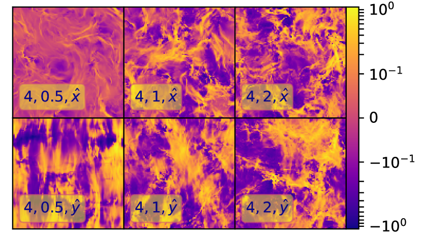
Figure 10: Projections of $E$ for the sonic mach $\mathcal{M_{S}}=4$ simulations, with targeted $\mathcal{M_{\rm{A}}}=0.5,1,2$. (Top row) projection along $\hat{x}$, with the magnetic field coming out of the page and (Bottom row) projection along $\hat{y}$, with the field pointing up (as in Fig. 1). Field strength increases to the left.

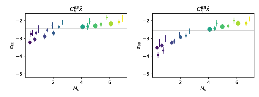
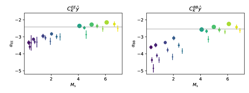
Figure 11: Amplitudes for $C_{k}^{EE}$ and $C_{k}^{BB}$ along the magnetic field ($\hat{x}$, top row) and across the field ($\hat{y}$, bottom row), as in Fig. 7.

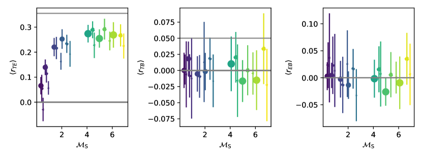
Figure 12: Average correlations $r_{TE}$, $r_{TB}$ and $r_{EB}$, left to right respectively, for the $\hat{x}$ projections along the magnetic field.

4 Conclusions

In this work, we examine the $E-$mode and $B-$mode spectra from a suite of idealized, magnetized, and turbulent simulations. We find that isothermal turbulence alone is enough to reproduce the observed values of $\alpha_{EE}$ and $\alpha_{BB}$, as well as the ratio of amplitudes, $A_{BB}/A_{EE}$, for suitable values of Mach number, $\mathcal{M_{S}}$, and Alfvén Mach number, $\mathcal{M_{\rm{A}}}$. We additionally find that the observed correlation of $T$ and $E$, $r^{TE}=0.3$, is naturally reproduced by the turbulence at high $\mathcal{M_{S}}$ and an appropriate magnetic field strength. Correlations with $B$ are spectrally flat and near zero, certainly below $0.05$, but the results are somewhat murky. We suggest that a “typical” patch of the sky has $\mathcal{M_{S}}=4.7$, $\mathcal{M_{\rm{A}}}=1.5$, based on linear interpolation of the $E$- and $B$-mode slopes, but $r^{\rm{TE}}$ prefers lower $\mathcal{M_{\rm{A}}}$ and higher $\mathcal{M_{S}}$.

The density spectrum is found to be tightly related to $\mathcal{M_{S}}$, with slope $\alpha_{\rho}\sim-3.6+0.16\mathcal{M_{S}}$. This is due to the fact that shock thickness decreases with $\mathcal{M_{S}}$, leading to smaller scale structure and faster growth of instabilities such as Richmeyer-Meshkov and Rayleigh Taylor. The velocity spectra is relatively insensitive to $\mathcal{M_{S}}$ for $\mathcal{M_{S}}<2$. Supersonic slope values cluster around $\alpha_{v}\sim-3.5$ for super-Alfvén values, slightly shallower than the Kolmogorov value of -11/3. Magnetic spectral slopes are relatively insensitive to $\mathcal{M_{S}}$, and decrease with decreasing magnetic field.

The projected quantities, $T$, $E$ and $B$, also depend on $\mathcal{M_{S}}$ and $\mathcal{M_{\rm{A}}}$. In these perfectly optically thin models, $T$ is the integral of $\rho$ along the line of sight, and it is found that $\alpha_{T}\sim\alpha_{\rho}$ with some small dependence due to the magnetic field. $E$ is found to depend on both $\mathcal{M_{S}}$ and $\mathcal{M_{\rm{A}}}$, from $\alpha^{EE}\in[-3.5,-2]$ and $\alpha^{BB}\in[-4.5,-2.2]$.

In Huffenberger et al. (2020), we model $E$ and $B$ with filaments that have an aspect ratio $\epsilon\in[0,1]$ threaded by magnetic fields at an angle, $\theta_{LH}$. It is found that as $\epsilon$ increases, the ratio of $B$ to $E$ increases as a longer filaments have proportionally more $E$. This also explains the decrease in $r^{TE}$ as $\epsilon$ increases. These predictions from the filament model are consistent with our findings with the turbulent boxes. As $\mathcal{M_{S}}$ and $\mathcal{M_{\rm{A}}}$ increase, the ability of the magnetic field to suppress instability decreases, and shorter filaments are expected. This can be seen in projections and in the power spectra of $\rho.$ Commensurate, we find an increase in $B/E$ and a decrease in $r^{TE}$ with increasing $\mathcal{M_{S}}$. Again, the shorter structures as a result of increased $\mathcal{M_{S}}$ and $\mathcal{M_{\rm{A}}}$ are in agreement, at least qualitatively, with the model of Huffenberger et al. (2020). Clark et al. (2021) model the parity violating correlation as a misalignment between filamentary structure and magnetic field direction in a similar filamentary framework, and compare to simulations. In future, we will examine filamentary properties of these cubes to further explore the predictive power of Huffenberger et al. (2020) and Clark et al. (2021).

In future simulation studies, we need higher resolution to increase our inertial range and improve our accuracy, particularly on the slopes. We also need larger statistical ensembles to quantify the sample variance in the $TB$ and $EB$ correlations. These are important for measurements of detector calibration, gravitational lensing, and cosmic birefringence.

References

- Beresnyak et al. (2005) Beresnyak A., Lazarian A., Cho J., 2005, ApJ, 624, L93
- Bohren & Huffman (1998) Bohren C. F., Huffman D. R., 1998, Absorption and Scattering of Light by Small Particles
- Bryan et al. (2014) Bryan G. L., et al., 2014, ApJS, 211, 19
- Caldwell et al. (2017) Caldwell R. R., Hirata C., Kamionkowski M., 2017, ApJ, 839, 91
- Clark et al. (2021) Clark S. E., Kim C.-G., Hill J. C., Hensley B. S., 2021, ApJ, 919, 53
- Collins et al. (2012) Collins D. C., Kritsuk A. G., Padoan P., Li H., Xu H., Ustyugov S. D., Norman M. L., 2012, ApJ, 750, 13
- Cukierman et al. (2023) Cukierman A. J., Clark S. E., Halal G., 2023, ApJ, 946, 106
- Dedner et al. (2002) Dedner A., Kemm F., Kröner D., Munz C.-D., Schnitzer T., Wesenberg M., 2002, J. Comput. Phys, 175, 645
- Diego-Palazuelos et al. (2022) Diego-Palazuelos P., et al., 2022, Phys. Rev. Lett., 128, 091302
- Diego-Palazuelos et al. (2023) Diego-Palazuelos P., et al., 2023, J. Cosmology Astropart. Phys, 2023, 044
- Federrath et al. (2008) Federrath C., Klessen R. S., Schmidt W., 2008, ApJ, 688, L79
- Federrath et al. (2010) Federrath C., Roman-Duval J., Klessen R. S., Schmidt W., Mac Low M., 2010, A&A, 512, A81
- Fiege & Pudritz (2000) Fiege J. D., Pudritz R. E., 2000, ApJ, 544, 830
- Goldreich & Sridhar (1995) Goldreich P., Sridhar S., 1995, ApJ, 438, 763
- Grete et al. (2023) Grete P., O’Shea B. W., Beckwith K., 2023, ApJ, 942, L34
- Huffenberger et al. (2020) Huffenberger K. M., Rotti A., Collins D. C., 2020, ApJ, 899, 31
- Kamionkowski & Kovetz (2016) Kamionkowski M., Kovetz E. D., 2016, ARA&A, 54, 227
- Kandel et al. (2017) Kandel D., Lazarian A., Pogosyan D., 2017, MNRAS, 472, L10
- Kim et al. (2019) Kim C.-G., Choi S. K., Flauger R., 2019, ApJ, 880, 106
- Kolmogorov (1941) Kolmogorov A., 1941, Akademiia Nauk SSSR Doklady, 30, 301
- Komatsu (2022) Komatsu E., 2022, Nature Reviews Physics, 4, 452
- Kritsuk et al. (2007) Kritsuk A. G., Norman M. L., Padoan P., Wagner R., 2007, ApJ, 665, 416
- Kritsuk et al. (2018) Kritsuk A. G., Flauger R., Ustyugov S. D., 2018, Phys. Rev. Lett., 121, 021104
- Mac Low & Klessen (2004) Mac Low M.-M., Klessen R. S., 2004, Rev. Mod. Phys. , 76, 125
- Meshkov (1972) Meshkov E. E., 1972, Fluid Dynamics, 4, 101–104
- Mignone (2007) Mignone A., 2007, J. Comput. Phys, 225, 1427
- Minami & Komatsu (2020a) Minami Y., Komatsu E., 2020a, Phys. Rev. Lett., 125, 221301
- Minami & Komatsu (2020b) Minami Y., Komatsu E., 2020b, Progress of Theoretical and Experimental Physics, 2020, 103E02
- Planck Collaboration et al. (2020) Planck Collaboration et al., 2020, A&A, 641, A11
- Pope (2000) Pope S. B., 2000, Turbulent Flows
- Rabatin & Collins (2023) Rabatin B., Collins D. C., 2023, MNRAS, 525, 297
- Richtmyer (1960) Richtmyer R. D., 1960, Communications on Pure and Applied Mathematics, 13, 297–319
- Towns et al. (2014) Towns J., et al., 2014, Computing in Science and Engineering, 16, 62
- Wang & Abel (2009) Wang P., Abel T., 2009, ApJ, 696, 96