Information propagation in far-from-equilibrium molecular templating networks is optimised by pseudo-equilibrium systems with negligible dissipation
Abstract
Far-from equilibrium molecular templating networks, like those that maintain the populations of RNA and protein molecules in the cell, are key biological motifs. These networks share the general property that assembled products are produced and degraded via complex pathways controlled by catalysts, including molecular templates. Although it has been suggested that the information propagated from templates to products sets a lower bound on the thermodynamic cost of these networks, this bound has not been explored rigorously to date. We show that, for an arbitrarily catalytic reaction network in steady state, the specificity with which a single product can dominate the ensemble is upper bounded, and the entropy of the product ensemble lower bounded, by a function of , the difference between the maximal and minimal free-energy changes along pathways to assembly. These simple bounds are particularly restrictive for systems with a smaller number of possible products . Remarkably, however, although constrains the information propagated to the product distribution, the systems that saturate the bound operate in a pseudo-equilibrium fashion, and there is no minimal entropy production rate for maintaining this non-equilibrium distribution. Moreover, for large systems, a vanishingly small subset of the possible products can dominate the product ensemble even for small values of .
I Introduction
Biochemical systems use catalysts to selectively produce multiple distinct products from a shared set of ingredients. For example, consider protein production [1]: many polypeptide sequences are created from the same set of amino acids, using a set of template mRNAs and other molecules act as selective catalysts [2]. The result is a distribution of polypeptide sequences in the cell, sharply peaked around the target sequences specified by the mRNA. Since these sequences fold into functional proteins, a sharply-peaked, or accurate, distribution is essential to biological function.
Often, biological systems continuously turn over the products, recycling the basic ingredients for subsequent use. For example, polynucleotide phosphorylase enzymes actively degrade the pool of selectively transcribed RNA [3]. Degradation allows the cell to set up a finite steady-state population that is biased towards specific products, and continuous turnover and recycling of components is necessary for systems with finite resources that need to change their state in response to dynamic environments. The underlying processes may also be complex and involve many possible routes of assembling and disassembling the products. For example, kinetic proofreading motifs [4, 5, 6] introduce fuel-consuming loops into the assembly process, thereby providing multiple pathways to each product.
Previous studies [7, 8, 9, 10, 11, 12, 13, 14, 15, 16, 17, 6, 18, 19, 20, 21, 22, 23, 24, 25, 26, 27, 28, 29, 30] have generally focused on models of a single production process only, in particular considering how templated copolymerisation in isolation can produce an accurate sequence. These studies have explored thermodynamic constraints on the accuracy in different classes of templated copolymerisation models, including those with single pathways leading to infinite-length polymers [23, 24, 25], more complex infinite-length polymerisation processes [26, 27, 28] and finite length copolymerisation [29, 30].
To the best of our knowledge, only Refs. [2, 31, 32] have considered the implications of two or more pathways for production and destruction of an ensemble of products, in each case without considering a detailed model of dynamical pathways. These works hypothesise a minimal thermodynamic cost or entropy production per product made, which is related to the information accurately transferred from template to products [2, 31, 32]. However, entropy production in stochastic thermodynamics is related to the relative rate of forwards and backwards transitions [33], rather than the relative rate of two different transitions; it therefore places no minimal cost on the specificity of a catalyst [29]. Exactly how these two ideas are reconciled is unclear.
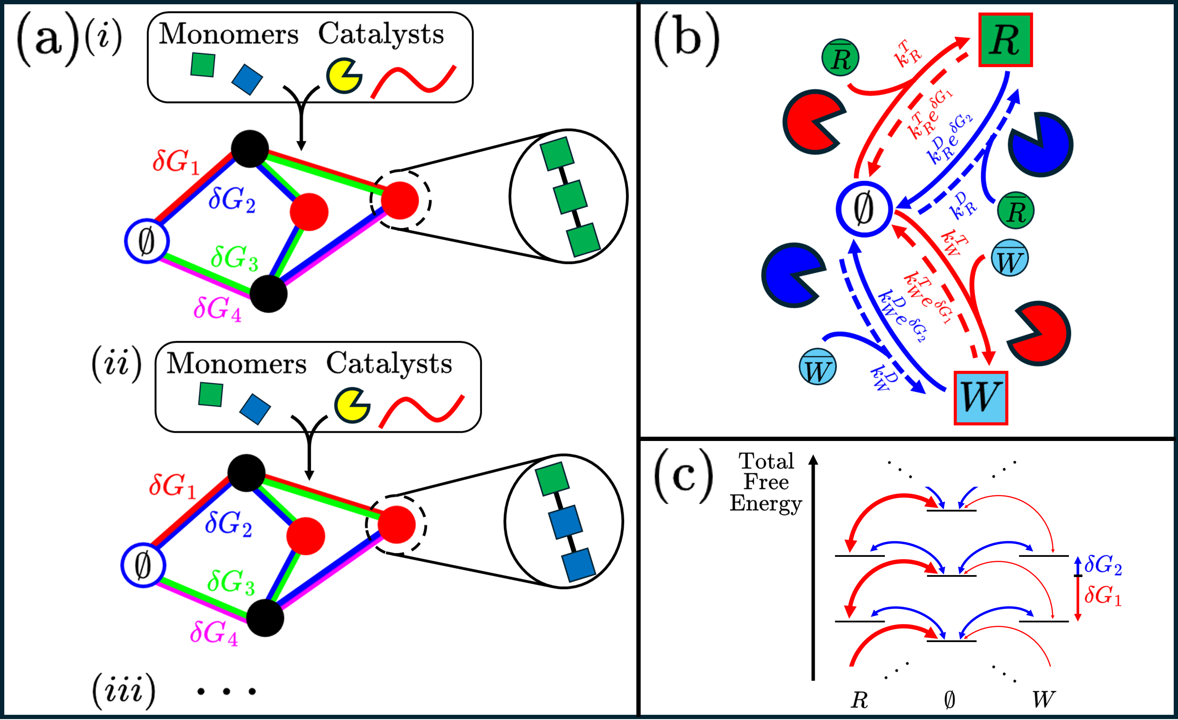
The limiting thermodynamics of this crucial class of processes therefore remains under-explored. In this paper, we consider the thermodynamics of a general system in which a distribution of products is created and maintained by a set of catalysts that inter-convert molecules between pools of monomer inputs and pools of assembled products. These inter-conversion processes can be arbitrarily complex, but we assume that all products have the same thermodynamic stability [2, 25, 29, 30, 32], consistent with the fact that catalysts cannot adjust the thermodynamic stability of the products that they select. Moreover, all products can be formed by a topologically equivalent set of processes (figure 1 (a)). By analogy with the processes of the central dogma, we shall loosely describe the catalysts that tend to generate products as “templates”, but we do not make any particular assumptions about the detailed mechanisms.
Each pathway for creating or destroying a given product can incur a different free-energy change (figure 1 (a)), due to coupling with ancillary fuel molecules. These free-energy changes specify the equilibrium that would result in the long time limit if that pathway operated in isolation. We will show that this set of equilibrium free energies sets a lower bound on the entropy of the product distribution in a non-equilibrium steady state, for any fuel-coupled catalyst-induced kinetics. If the system is interpreted as an information channel between the input catalysts and the output products, this lower bound on entropy is equivalent to an upper bound on channel capacity [34, 35].
The bound on product distribution entropy also sets a bound on the accuracy with which a single product can dominate the resultant ensemble. But surprisingly, the goals of producing a distribution maximally specific to a single chemical species and producing the distribution of products with minimal entropy are generally distinct. Moreover, contrary to our expectations, the optimal system that minimizes the entropy of the product distribution – pushing the distribution as far from equilibrium as possible – is not one in which desired products are systematically assembled on a template and degraded by another catalyst [31]. Rather, the optimal system is a pseudo-equilibrium one in which kinetic specificity ensures that each product is coupled overwhelmingly to only a single pathway, with each product’s yield specified by the equilibrium properties of that pathway.
Exploring our bound, we observe that, for possible products, it is possible to selectively produce a single product with perfect accuracy in steady state provided two pathways exist that are separated by in their free-energy change, irrespective of other pathways. However, the probability of producing a single correct product as is zero for . Further, the convergence to the infinite behaviour is slow. Similarly, zero entropy product distributions can never be achieved with finite , but even low entropy requires .
These results appear consistent with the notion that accurately maintaining a specific pool of products has a thermodynamic cost related to the information stored ( if a single template selects for a unique product) [31, 2, 32]. However, this simple picture is incomplete. Since the bound is saturated for pseudo-equilibrium systems in which each product couples overwhelmingly to a single pathway, there is no minimal entropy production per product molecule created in these steady states. Moreover, for , although a single product cannot be maintained with any accuracy for , it is possible to maintain a vanishingly small fraction of the total possible products with perfect accuracy for any , even if . Finally, the bounds only apply to steady states, and it is possible to produce distributions of arbitrary precision at finite time with no minimal .
In Section II, we formally introduce the class of models and techniques used to analyse them. In Section III, we motivate our analysis by considering the simplest possible case of a network of this kind, in which two products can both be produced via two pathways. We find that, even with full control over the forward fluxes of each reaction, the concentrations of each product are still constrained by the equilibrium properties of the individual pathways. In Section IV.1, we then derive bounds on the distribution of products for a more general class of models that include multiple, sometimes overlapping creation and destruction pathways to an arbitrary number of products. In Section IV.3, we discuss the physical interpretation of the bounds. Finally, in Sections V.1 and V.2, we explore how systems are constrained by the bound in two biologically inspired examples. Throughout this article, we shall use Shannon entropy in units of nats, free energies in units of , and concentrations relative to a reference concentration. Additionally, we use the symbol “” to mean “less than something which is approximately equal to” and similarly for “”.
II Models and methods
II.1 Physical model
We now define the class of models considered, illustrated in figure 1 (a). Consider a set of input chemical species that may be assembled into a number of different possible products. For simplicity, and to focus on information propagation, we shall assume that all input species are held (chemostatted) at the same constant concentration by the cell or the environment. In these context of the central dogma of molecular biology, these inputs would be the nucleotides or amino acids. There are possible different products that these inputs may form, corresponding to the different sequences of copolymers (e.g. RNAs, polypeptides). Finally, there are catalytic species (e.g. templates, polymerases, or nucleases) that facilitate the inter-conversion of inputs and products via intermediates. We assume that these catalysts are also chemostatted, and neglect any reaction involving more than one product and/or intermediate. We are interested in the set of products formed.
Such a model may be expressed as a deterministic chemical reaction network (CRN) [36, 37]. A deterministic CRN consists of a set of chemical species, a set of complexes (which are collections of species), and a set of reactions. In each reaction, a complex (the set of reactants) is converted into a different complex (the set of products) at some reaction rate, which is a function of the concentrations of species making up the reactants. We shall work with deterministic reversible CRNs obeying mass action kinetics. By reversible, we mean that, if a reaction from a complex to a complex is allowed, then its reverse reaction from to is also allowed. By mass action kinetics, we mean that the rate of a given reaction is proportional to the product of concentrations of species making up the reactants. Henceforth, we shall refer to the constant of proportionality as the “reaction rate”. Since all reactions are reversible, we may use the principle of local detailed balance to define free-energy changes due to reactions. For a pair of reactions , with reaction rate , and its reverse with reaction rate , the free-energy change due to this reaction is
| (1) |
Given our assumptions about their chemostatting, the concentrations of input species and catalysts can be treated as parameters, rather than variables. Under such assumptions, the CRNs are linear: the set of complexes contains only the null complex (containing no non-chemostatted species), and singletons (containing a single non-chemostatted species, i.e. an intermediate or a product). All reaction rates therefore depend linearly on the concentration of the non-chemostatted species. Transitions from the null complex correspond to the first association between inputs or inputs and catalysts to produce an intermediate.
We can draw a linear CRN as a graph (e.g. figure 1 (a)(i)), with nodes as species, edges as reactions and weights as reaction rates, absorbing the concentration of any chemostatted species involved into the reaction rates. We shall assume the graph produced is connected, as it must be if all species can be produced from the null state. This graph defines a set of self-avoiding walks (SAWs) from the null state to each product; each SAW together with its inverse define a “pathway” between the null state and the products.
We allow for the transitions to be coupled to implicit fuel molecules, meaning that different SAWs are associated with different . However, each edge must correspond to the turnover of a fixed number of fuel molecules; branching pathways allow for variable fuel consumption when coupled to a given catalyst. Each SAW from the null complex to a product therefore has a well-defined free-energy change.
We assume that products are all connected to the null complex by topologically equivalent graphs (figure 1 (a)). Such an assumption makes sense for a set of products corresponding to, for example, RNA molecules of a fixed length, which can all be grown via an equivalent set of steps. We further assume that all products are equally thermodynamically stable. This assumption is consistent with the fact that catalysts cannot thermodynamically favour one product over another [2, 25, 29, 30, 32], and allows us to focus on the question of how information is propagated from catalysts to products. Any internal thermodynamic bias towards certain products would not generally help to form an arbitrary product.
As a consequence, the equilibrium product state would contain a uniform distribution over products [2] and a narrower distribution over products can only be achieved via kinetic selection of a non-equilibrium steady state by the catalysts. Moreover, there exists a finite number of SAWs from the null complex to any given product, each with a free-energy change where indexes the given SAW. The set of SAWs from the null complex to any product will be topologically equivalent and incur the same set of total free-energy changes (figure 1 (a)).
These constraints on free energy only apply to full paths from the null state to completed products. Intermediate states, involving partial, catalyst-bound products, can have sequence-specific free energies. Moreover, the transition rates between states can be different, subject to the overall constraint that, along a given complete SAW from null to product, the total free-energy change is the same as its equivalent for all other products. We will explore how relative yields of the products can be optimised by varying these strictly positive rates arbitrarily under this constraint.
Finally, we focus on deterministic CRNs here. However, since the CRNs are linear and connected, our results also apply to the expected concentrations at steady state of a stochastic realisation of the CRN [38].
II.2 Analytical methods
The steady state concentration of species in a linear, deterministic CRN can be found directly from the graph. The concentration is given by the ratio of the sum of spanning trees of the graph rooted at the species to the sum over spanning trees rooted at the null species. Explicitly,
| (2) |
where is the set of spanning trees rooted at node , is an edge in graph , and means the weight of edge . For a proof, see appendix B or [39] for a similar result.
These sums over spanning trees may be usefully rewritten as a sum over the SAWs from the null species to the given product species [40, 28]. Having done so, the results are expressed in terms of the free-energy change along a given SAW [36] ,
| (3) |
where is the reverse reaction of edge . Note that SAWs with positive correspond to pathways that tend to disassemble products.
Using graph theoretical methods, one may calculate the steady state concentrations for all of the product species. Having done so, and denoting the products by for , we define the product distribution as the probability that a randomly chosen product from the resultant ensemble is ,
| (4) |
where is the total concentration. We define the (Shannon) entropy [35] of this distribution as
| (5) |
In appendix A, we show how under certain assumptions, the minimisation of this entropy maximises the channel capacity of this system if treated as an information channel from catalysts to products. Informally, a lower entropy reduces the probability that the same product is sampled from the output of two different catalyst configurations.
II.3 Simulation of specific networks
Although calculations of the bounds (section IV.1) is often straightforward, evaluation of the actual performance of a system realisation can be more challenging. For the examples presented in section V, steady state distributions are found by numerical solutions of the underlying ordinary differential equations (ODEs). The CRNs are linear, connected and contain only one stoichiometric compatibility class. Hence, there exists a single positive steady state to the ODEs induced by mass action kinetics [36]. Initially, all concentrations are set to zero, and the ODEs are simulated for a large time until no change to the distribution is observed. For section V.2, to speed up simulation, we make use a of a result from [28] whereby we may coarse grain some sets of reactions without changing the steady state. The code used to simulate the ODEs is available from the zenodo repository.
III Free-energy differences between pathways bound accuracy for a simple network with two catalysts
To build intuition, we first consider the simplest non-trivial system in which inputs and products are inter-converted by catalysts (figure 1 (b,c)). The reaction network has two product species that we denote “right” () for the target species and “wrong” for the other species (). These products are formed by catalytic activation of their inactive states and , which are the input monomers, present at equal concentrations. Absorbing the concentrations of and and the catalysts into the rate constants, we may describe the system via the following CRN:
| (6) |
where is the null species, and the effective reaction rates are written above/below the arrows. For each product there are two pathways from the null state leading to the product, one via a catalyst we call the template (reaction rates labelled by in equation 6) and one via a destructive catalyst (reaction rates labelled by in equation 6). For simplicity, we have assumed the catalyst-bound intermediates are short-lived, and do not explicitly represent them.
The pathways via the destructive catalyst are both biased with free energy against creating the product, relative to the pathways via the template (). A non-zero implies that the (or ) pathway is coupled to the turnover of implicit molecular fuel, allowing the apparent disruption of detailed balance [33]. Each individual pathway, however, has a well-defined free-energy change associated with it; in the presence of only that pathway, the system would relax to an equilibrium defined by the free-energy change of that pathway.
The two products and can be produced by topologically equivalent pathways, by processes with the same overall free energy change. and are therefore both equally thermodynamically stable and a non-equilibrium excess of over is only possible if the template is kinetically selective for production of over . This setup is a minimal analog of a transcription-like system in which all products are thermodynamically viable, but those selected by the presence of their templates are preferentially produced.
In a conventional analysis of a system in which a template selectively produces a specific daughter molecule [9, 10, 11, 12, 13, 14, 15, 16, 17, 18, 19, 20, 21, 22, 23, 24, 25, 26, 27, 28, 29], it is typical to simply consider how selective the template is when producing the intended product. We can calculate the net flux of product, , along pathway in steady state as
| (7) |
where is the concentration of . Equivalent equations have the same form for , , and . At the steady state, for .
By varying the underlying rates at fixed , the flux ratio relating the production rate of and by can be straightforwardly varied. A quick calculation shows that this ratio is
| (8) |
This ratio can be made arbitrarily large for any , simply by picking appropriate rates , forcing the template to produce output at a rate arbitrarily higher than the rate it produces output . The catalyst can therefore be arbitrarily kinetically selective for a given along each pathway; kinetic selectivity of catalysts is not – in principle – constrained by thermodynamics.
We might, therefore, expect to be able to produce an output distribution that contains an arbitrarily higher concentration of than by varying the reaction rates at fixed . However, this is not the case. The steady-state concentrations of and are
| (9) |
Both these concentrations are bounded by . Hence, we cannot achieve an arbitrary ratio of concentrations, . Moreover, since ratios and can be set independently, an arbitrarily high ratio of fluxes does not necessarily correspond to a high ratio of concentrations. For example, if the rates obey (figure 1 (c)) then will be large, and will be close to . However, if instead , then will still be close to , but will be small.
The optimal distribution giving the highest proportion of the right product is found when and . In this case, is overwhelmingly produced and destroyed via the template. For , it is as if the yield is governed by the equilibrium of a single red transition in figure 1 (c). , by contrast, is overwhelmingly produced and destroyed via ; its yield is equivalent to the equilibrium of a single blue transition in figure 1 (c). This “pseudo-equilibrium” limit gives a concentration of for and a concentration of for . We note that although the individual products appear to equilibrate, the product ensemble remains far from equilibrium, because different product species are coupled to different equilibria.
In conclusion, even with arbitrary relative fluxes of different products along different pathways, and a far-from-equilibrium distribution of products, the relative steady-state concentrations of products are bound by the differences in the equilibrium properties of individual pathways, and the ideal behaviour involves vanishing cyclic flux around the template/destroyer cycle. In the remainder of this paper, we shall generalise this result and explore its consequences.
IV General Bounds on the properties of product distributions
IV.1 Derivation of the bounds
We shall now present the main mathematical results of this work: an upper bound on the maximal probability of a single product , and a lower bound on the entropy of the product distribution. To do so, we first note that for the class of linearised CRNs considered here, the steady-state concentration of any species is bound by the set of free-energy changes along the pathways that create or destroy it. Generalizing the result in Section III, the steady state concentration is upper-bounded by the equilibrium implied by the single pathway with the most negative free-energy change of species formation, and lower-bounded by the equilibrium implied by the pathway with the most positive free-energy change of species formation. These bounds are achieved when the rates along all other pathways tend to zero.
Mathematically, we define and as the maximal and minimal free energy changes along self-avoiding walks that lead to the creation of from the null state, respectively. Then
| (10) |
The proof for this statement is given in Appendix C, although similar bounds are shown in [41, 42, 39, 40].
Our systems have the particular property that the concentrations of all product species have the same upper and lower bounds (). As a result of this crucial fact, properties of the distribution defined by eq. 4 are constrained. Specifically, the maximal probability of a single product has a non-trivial upper bound, while the entropy has a non-zero lower bound. We now calculate the optimal distribution for maximising one desired product and the distribution for minimising total product distribution entropy, showing that they are different.
When maximising the probability of a single product species, hereafter referred to as specificity maximisation, the probability distribution will be one product with probability , and all others with , with
| (11) |
where and is the number of possible product species.
Alternatively, we can consider entropy minimisation, or finding the minimal entropy of a distribution under the constraint that all species are restricted by . We obtain , with
| (12) |
arises from a distribution in which species are at the upper bound concentration, , and species are at the lower bound, . The that minimises entropy is given by either:
| or | |||
| (13) |
whichever gives the lower . We use the ceiling function because is integer; we are required to check two values on either side of the minimum of the continuous function. A reasonable approximation to the optimal value of is given by
| (14) |
since for , the difference between using the integer value of (eq. 13) and the continuous value (eq. 14) is small. In practice, using equation 14 produces a very slightly looser bound on . Further, using eq. 14, for , we may simplify:
| (15) |
The proofs for these results are given in appendix D. Note that in the context of copolymerisation, is proportional to the length of polymer necessary to produce different possible product sequences.
IV.2 The bounds in the presence of kinetic proofreading
Surprisingly, internal cycles in the reaction network, a requirement for celebrated kinetic proofreading motifs [4, 5, 6], do not directly feature in the bounds derived, since SAWs cannot contain cycles by definition. Adding a proofreading loop to a process may affect , since it may provide a new pathway with a maximal or minimal free-energy change, but the SAWs identified would always be loop-free and correspond to a fixed free-energy change for product formation. The possibility of repeatedly undergoing a single dissipative cycle in an actual dynamic trajectory, consuming an arbitrary amount of molecular fuel, does not translate into an arbitrary along a pathway. However, the existence of loops within the network may still help to achieve a better product distribution than otherwise if transition rates are constrained beyond the free-energy changes along SAWs being fixed.
IV.3 Physical significance of the bounds
We split the analysis into three main parts. In the first, we discuss the difference between specificity maximisation and entropy minimisation. We look at the properties of both of these distributions in detail. In the second we compare our result to the previous arguments from Bennett on the minimal cost of systems that create product polymers via templates and destroy them via other pathways [31]. Finally, we discuss whether and how systems can, even in principle, reach the bounds we find.
IV.3.1 Entropy minimisation versus specificity maximisation
One might naively expect that the distribution of product concentrations that minimises the entropy would be the same as the distribution that optimises the probability of a single product. However, this is not the case in general. The concentration of each species is constrained between and . The lower concentration cannot be arbitrarily close to zero, and the higher concentration cannot be arbitrarily high. Since having multiple products at the high concentration increases the total concentration of products, suppressing the relative probabilities of sampling products at the low concentration, the probability distribution may be sharper for systems with multiple products at a higher concentration. In this subsection, we first discuss when specificity maximisation and entropy minimisation are equivalent; then proceed to analyse specificity maximisation and finally entropy minimisation.
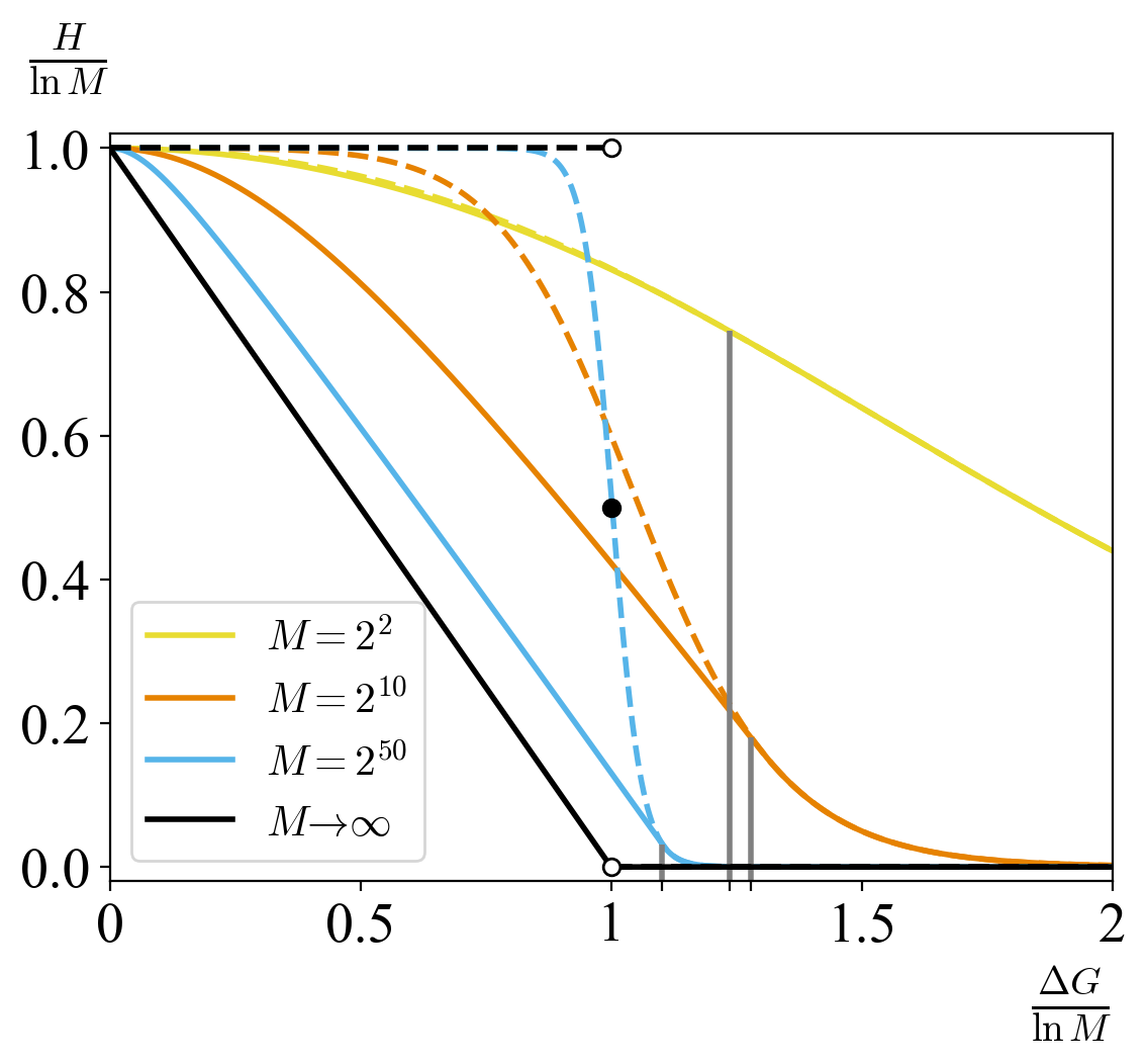
If minimises eq. 12, entropy minimisation and specificity maximisation are equivalent. The lowest entropy state then contains a single product at a high concentration, and all others at a low concentration. We find is optimal for (figure 2). For smaller than this value, the entropy of the distribution that maximises specificity differs quite drastically from that minimising the entropy. Surprisingly, the distribution for maximising specificity has an entropy consistent with an unbiased distribution () for in the limit . In other words, the concentration of the desired product tends to zero relative to the total concentration of products.
To explore this observation further, we consider the maximal product probability . The probability is a sigmoidal function centred on , with at and as . Interestingly, the sigmoidal function does not approach a step function here, but has fixed width around (figure 3a). Instead has the exact form as . Thus, if we were to plot as a function of , the curves for different, but large enough, would collapse onto each other. Therefore, to achieve a for small , one needs a . If we instead scale by system size, we find that tends to a step function when (figure 3b), reiterating that the relative yield of a single product is necessarily zero below as . Although the intended product can be far more probable than any single alternative, the large number of possible alternatives dominates.
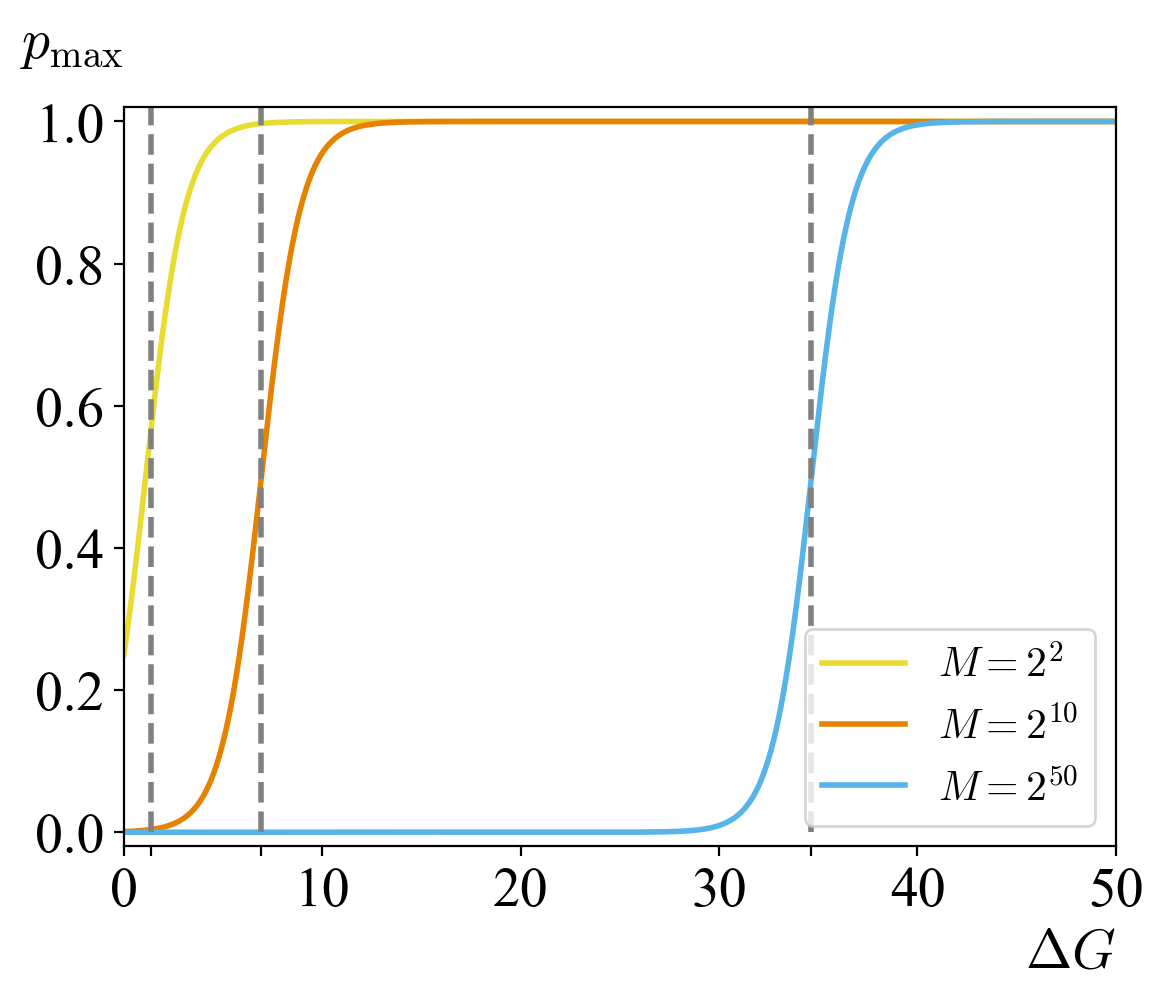
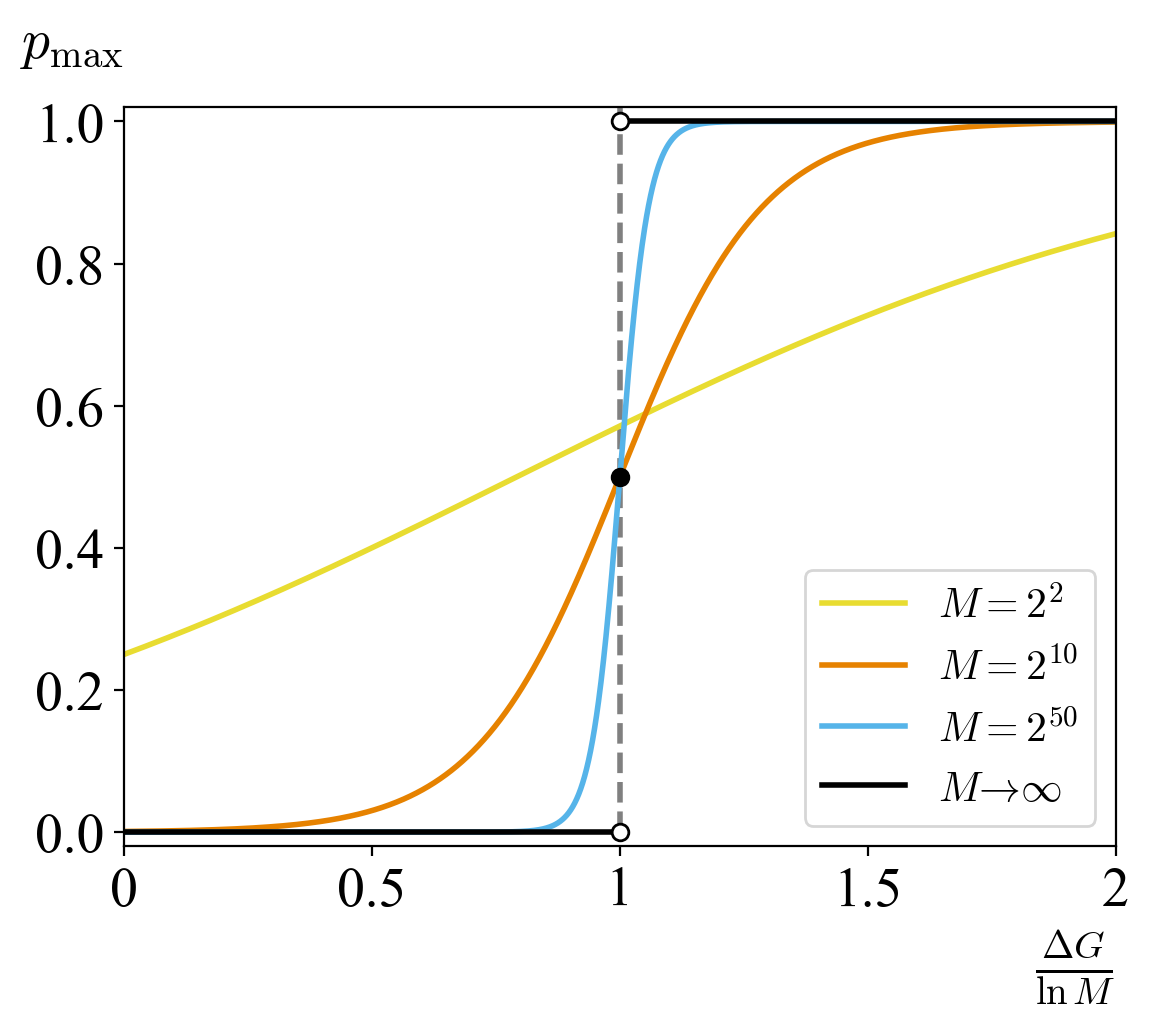
To put the bound on into context, we consider the implications for the charging of a single tRNA with the correct amino acid. Here, there are approximately different combinations of codon and amino acid, having grouped all codons that correspond to the same amino acid into one. Using , we can calculate the bound for the specificity with which an ensemble dominated by a single charged tRNA could be maintained in steady state. We see that for an error rate of , i.e. , one needs a free-energy difference in the pathways connecting inputs and products of approximately . Thus, for an error rate of , one would need a free-energy difference of around or 1 ATP[43] at , substantially higher than , the value implied by the large limit.
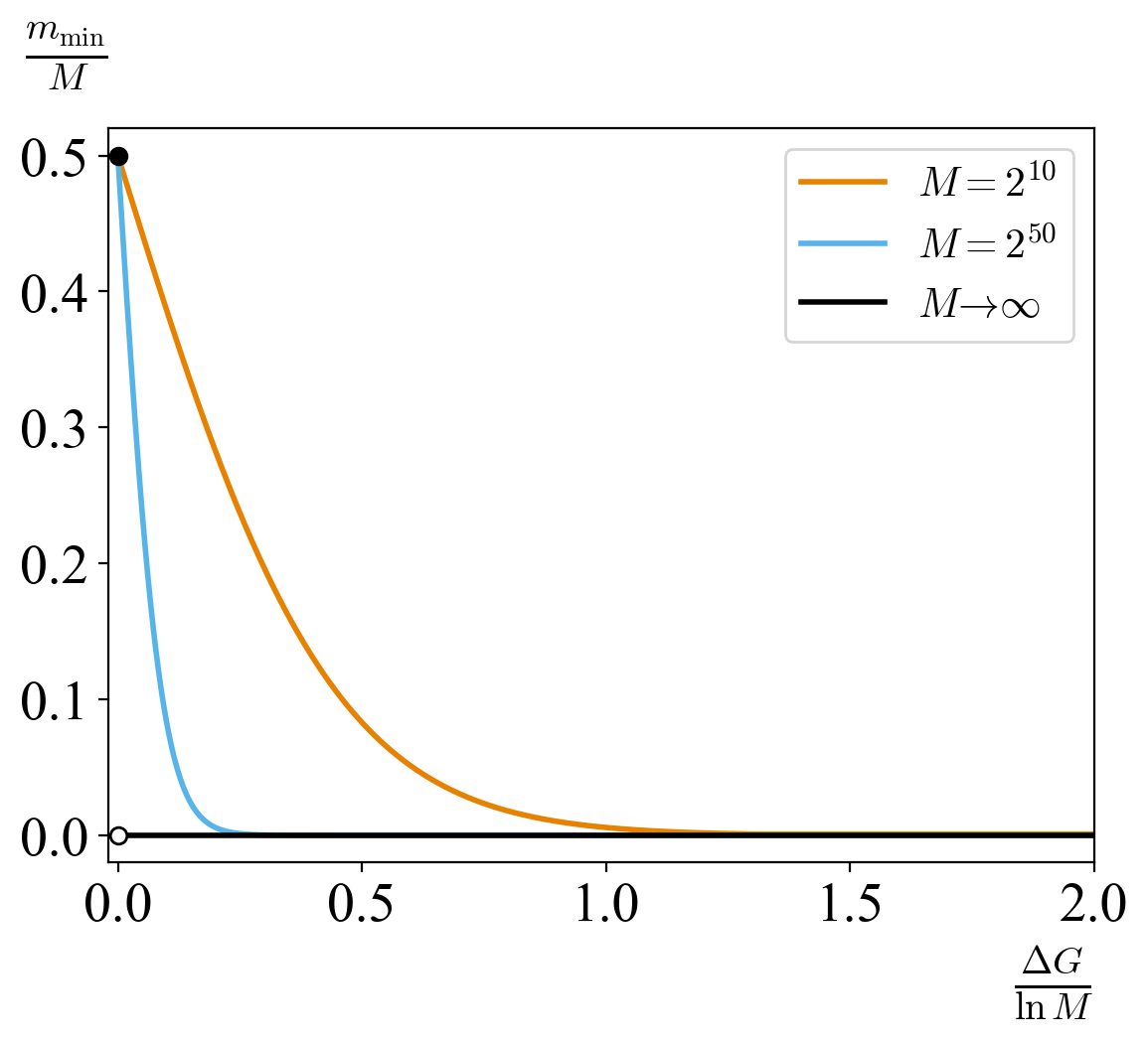
For entropy minimisation, we find that the limits and are identical to those found by specificity maximisation (figure 2). At , all pathways carry the same free-energy change and so the system is a true equilibrium one and no specificity is possible, . For , for all and a single product dominates. As can be seen from figure 2, the approach to the limit is very slow. Even for , there is a significant discrepancy between and the minimal entropy for the limit. This difference, when normalised by , is approximately (which is for ).
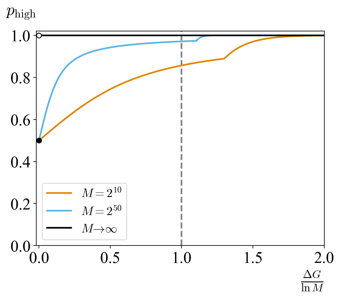
We now consider the properties of the entropy-minimizing distribution for . Here, species are at the same high concentration, and the remaining species are at a low concentration. The fraction given by eq. 14 is independent of , and monotonically decreases to with increasing . Thus, if we scale at fixed , the fraction of products with high yields will tend to zero even for , well inside the region where specificity for a single product is impossible (figure 4a).
Furthermore, the probability of a product randomly chosen from this distribution being one of the with a high concentration is given by . This quantity is also independent of and increases monotonically with to (figure 4b). Thus, as at fixed , a vanishingly small proportion of the total number of products can contain an overwhelming majority of the probability, even for and . The black lines in figure 4 illustrate this surprising phenomenon in the limit of .
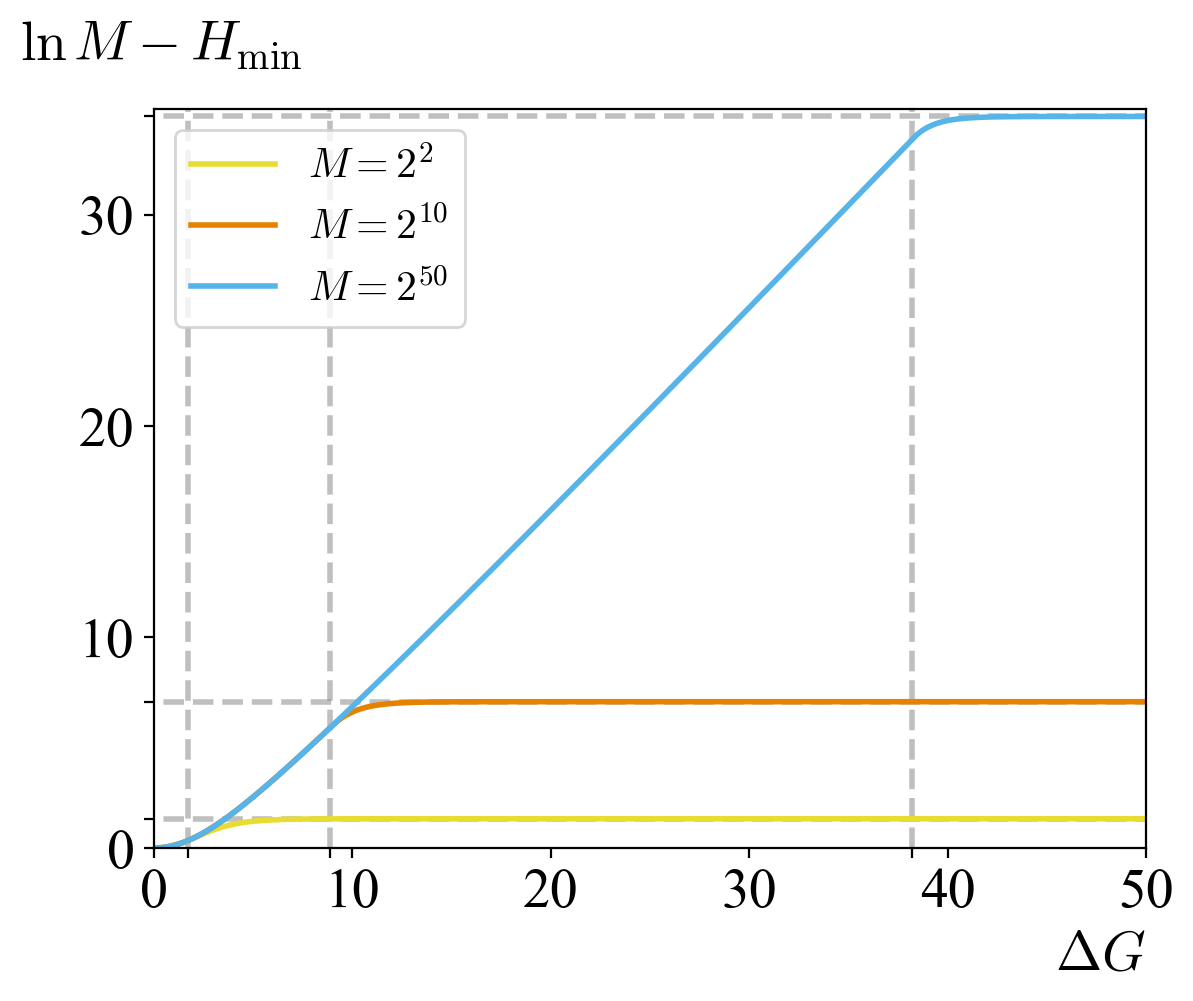
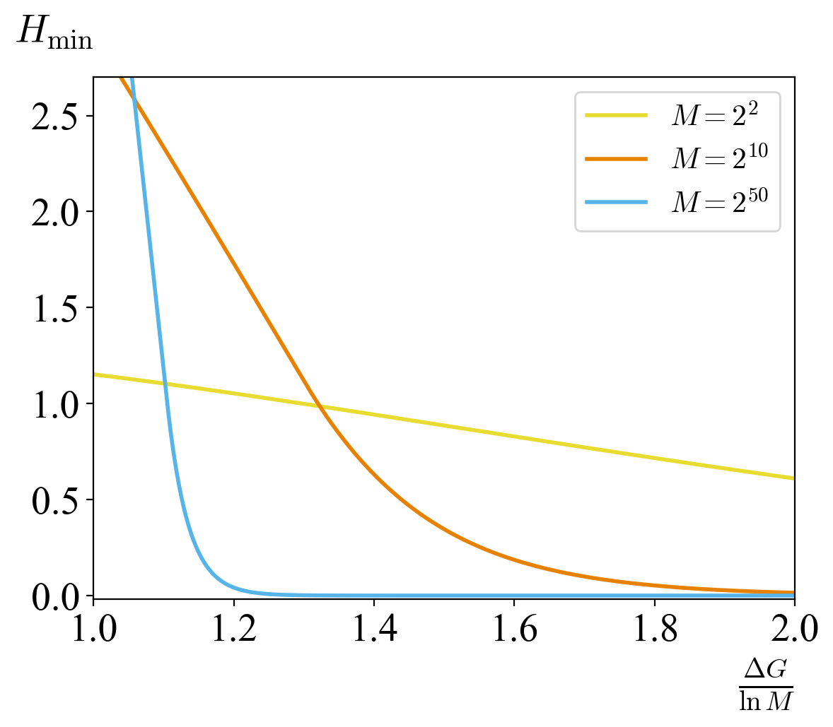
Turning now to , we consider how behaves for large and large, but finite, . Below , from eq. 15, , which is approximately linear in (figure 5a). Above , decreases exponentially as . Further, at , . Since the maximum value of is , this value for gives the approximate scale for to be considered small.
In figure 5b, we show how the limits on the un-normalised entropy vary with . Here, for sufficiently large , increasing leads to a nominal decrease in , not just a decrease in , as might be expected. Similarly for specificity maximisation (figure 3a), for sufficiently large , increases with increasing . Longer polymers therefore have much more scope within the bounds derived to use a given per monomer to suppress the absolute entropy of the resultant product distribution.
IV.3.2 Relationship of the bounds to previously postulated costs
In his seminal paper [31], Bennett briefly discussed the production of a single product RNA copolymer using a specific template, and its subsequent destruction via a non-specific destructive enzyme. Without considering a specific model, he stated that since the enzyme is nonspecific, one requires four times the phosphate concentration driving the non-specific destructive enzyme than one would if it was a sequence-specific destructive enzyme. This difference would prevent the non-specific destructive enzyme from creating non-target, random sequences, instead encouraging it to indiscriminately destroy everything, including the target sequence. He therefore states that a cycle of create via template followed by destruction via destructive catalyst must use at least per nucleotide of free energy, even in steady state, corresponding to in our formalism.
Our bounds update this understanding in several ways. Firstly, we point out that although two pathways with are required to generate a product distribution consisting of a single sequence in the steady state, the optimal system in terms of maintaining a specific product pool would not typically push polymers around a cycle, producing of entropy each time a polymer was created then destroyed. Instead, although the distribution over products as a whole is far from equilibrium, each product is effectively in its own kinetically-selected pseudo-equilibrium state. Each product is produced and destroyed by inverse pathways coupled to the same type of catalyst. Such a system has vanishing entropy production per creation event in the steady state.
Secondly, as shown through figures 2 and 3, while does serve as a necessary condition for perfect specificity in the limit of infinite polymer length, the approach to this limit is slow. A finite size correction on the order of (where would be the length of a polymer product) provides the minimum free-energy difference above for high specificity to be achievable.
Thirdly, the bounds are fundamentally a property of distributions of products and monomers, rather than the specificity of templates [29]. Although the kinetic selectivity of the template is important in determining how close a system can get to the bound (see section V), it doesn’t set the bound. This observation resolves the paradox that there are thermodynamic constraints on the templated ensemble, even though there are no thermodynamic constraints on catalytic specificity.
That the bounds are unrelated to catalytic specificity is particularly emphasised by considering the region . In this region, for large , a fraction of the possible products dominates the ensemble. In principle, such an ensemble could follow from distinct templates each catalysing formation of a single product sequence with high accuracy, even for . Intriguingly, for , a vanishingly small fraction of the possible products can constitute the full ensemble, in the absence of any other products, even for .
Fourthly, the limits on entropy and specificity with hold not only in the case of a non-specific destructive ecatalyst but also for a specific one, or indeed any complex set of pathways between monomers and products.
Finally, although our work mainly focuses on the issue of creating a steady state distribution of high specificity, we note by simple example that away from steady state, no free-energy differences are required to achieve arbitrary specificity. Consider a simple system with two products as follows:
| (16) |
This CRN is a simplified version of the system considered in section III, with only a single catalyst and thus . The steady state bound on this distribution would give an unbiased equilibrium of . However, the concentrations of and can be very different at short times. Starting with initial conditions ,
| (17) |
which is only bounded by 0,1. Thus, the entropy can temporarily be below our steady-state bound and we can achieve arbitrarily high specificity for any set of free-energy differences between pathways.
IV.3.3 The achievability of the bounds
The bounds we have derived are not always achievable, even if we allow a system to have arbitrary reaction rates consistent with the overall of each path. Whether or not the bounds are achievable depends on the topology of the CRN. To achieve the bounds, it is essential that it is possible to make the pathways corresponding to for high-yield products and for low-yield products fast, while keeping all other pathways slow. Given that pathways to a product will typically share edges with pathways to other products, this independent scaling is not always possible.
A pleasing aspect of our result is that, although finding full steady-state concentration requires knowledge of all of the SAWs from to the product, identifying the bounds only requires knowledge of the pathways with the highest and lowest free-energy-change. These free energy changes can often be intuited or proven without knowing all of the pathways. Further, it is then often possible to check whether or not the set of pathways identified is indeed compatible with reaching the bound.
V Examples
Having explored the properties of the bound itself, we consider two example systems to see how/whether the bound is reached as the rates along different edges are extremised.
V.1 Example 1: Templated polymerisation with a destructive catalyst
Refs [25, 28] studied a system in which a polymer is grown on a template. Monomers of either the “right” or the “wrong” type are added one at a time to a polymer in contact with a template, while the product polymer continually unbinds from the template from behind its leading edge. We now extend the system to include final dissociation from the template for complete polymers, and also a “destructive template”. This destructive template participates in identical reactions to the template, except that polymerisation is driven backwards due to consumption of fuel molecules, meaning products tend to be destroyed rather than grown.
A full CRN for this model is shown in appendix E; we illustrate the linearised network (assuming monomers and catalysts are coupled to chemostats) for the case of dimerisation in figure 6. The thermodynamics of the model are characterised by the standard polymerisation free energy of the monomers (); the standard free-energy change of binding to the template for right and wrong monomers ( and ), and the free energy of fuel turnover . We assume that both right and wrong monomers are held at concentration .
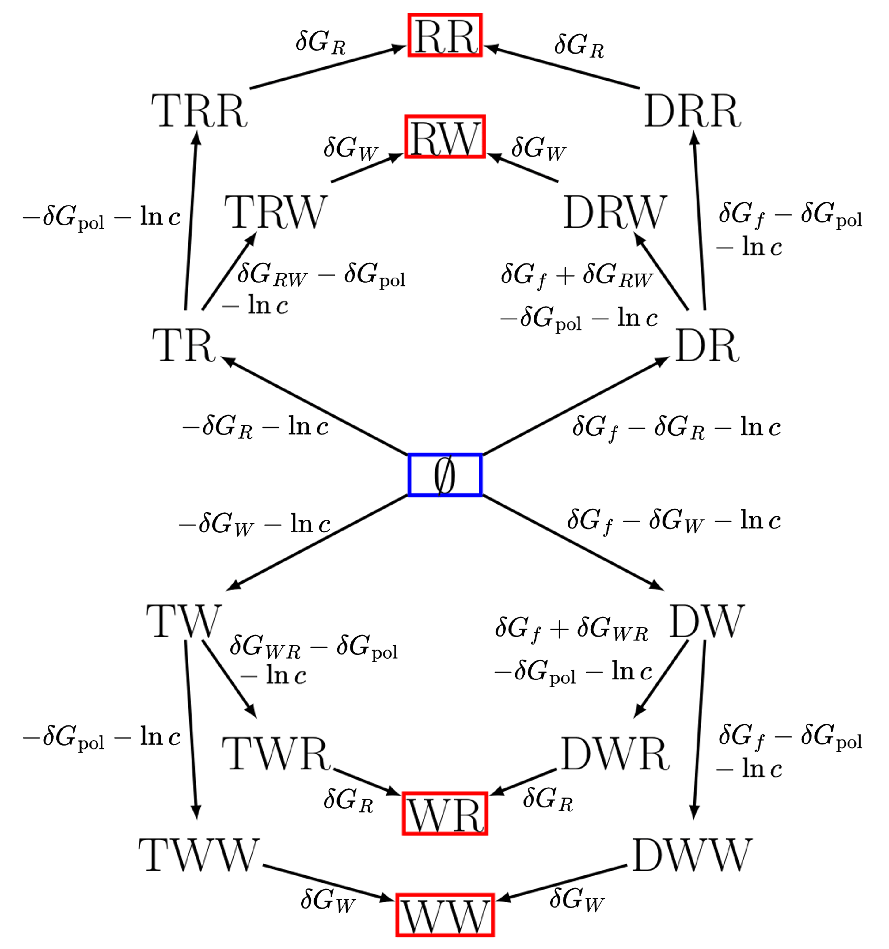
For the model depicted in figure 6, we can calculate the free-energy change for different paths to each product state. For example, the paths from the null state to are:
| (24) |
These incur free-energy changes:
| (25) |
Each pathway contains the terms , corresponding to the standard free-energy change of product formation without any fuel turnover. Since our bounds only rely on the differences in free energies between pathways, we may drop these contributions, and the fuel free energy alone determines the bounds. For polymers of length , the equivalent standard free energy of product formation is , and it too may be dropped for consideration of the bounds.
Our bounds are achieved when rates of the path with the most negative free-energy change are maximised for the desired product(s), and rates of the path with the most positive free-energy change are maximised for all other products. For the case, for example, we could therefore maximise the rate of path 1 for , and the equivalents of path 4 for other products.
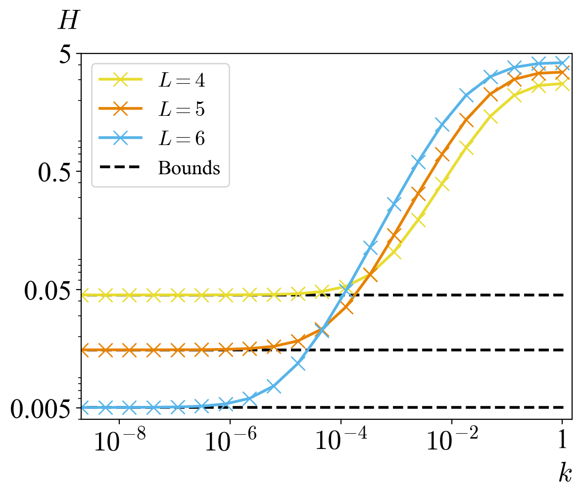
In fact, for this system, the entropy bound is formally achievable for arbitrary . We can split the edges of the graph into two sets; one in which the rates are , and one in which the rates are . In figure 7, we show as for a particular choice of these sets, in which all the reactions leading directly to the fully correct sequence being created/destroyed on the template are set to be fast (not proportional to ), as are all the reactions leading directly to the creation/destruction of other sequences on the destroyer. The system saturates the entropy bound found in section IV.1 as . Note that for the value of used, the minimal entropy and maximal specificity distributions are the same.
There are many possible ways to chose sets of edges that can saturate the bound in the limit . Here, we have chosen a set of rates that specifically highlights a full pathway to each product for illustrative purposes. One might also wish to choose a minimum set of rates to have rate while still saturating the bound in the limit . For example, letting the slow reactions be , where means copies of , and , excluding all being (appendix E), will still saturate the bound in the limit . Further, we note that it is possible to saturate the bound with a non-specific destructive catalyst, where the reaction rates are independent of the polymer sequence. In the examples we have identified, such a network requires at least three rate scales .
We stress that although the bound is formally attainable in this system, doing so relies on the ability to manipulate rate constants arbitrarily, subject to thermodynamic constraints. In a more realistic model of a templating system, constraints on relative rates may also be relevant; these constraints may stop the system reaching the bounds on accuracy or product entropy.
V.2 Example 2: Hopfield-like kinetic proofreading with a destructive catalyst
To illustrate the application of the bound to a more complex network, and to demonstrate the possibility of non-trivial pathways defining the bound, we consider an extension to the previous model, wherein the template also performs kinetic proofreading. First suggested by Hopfield [4] and Ninio [5] and widely studied [6, 44], kinetic proofreading is a mechanism by which a system can increase the specificity of a process by expending extra free energy through fuel consuming cycles. These cycles give an extra opportunity to reject the “wrong” monomers due to their shorter binding lifetime.
The full chemical reaction network for a proofreading template of arbitrary length is given in appendix F. Once again, we linearise the system by assuming that monomers and catalysts are coupled to chemostats. In figure 8, we show part of the linearised CRN graph; this fragment should be inserted into figure 6 in place of the pathway (), with similar modifications to all other template-based pathways to , , and . Proofreading adds complexity to the graph in the form of additional loops, and we now explicitly consider a polymerization step independently from the binding to the template.
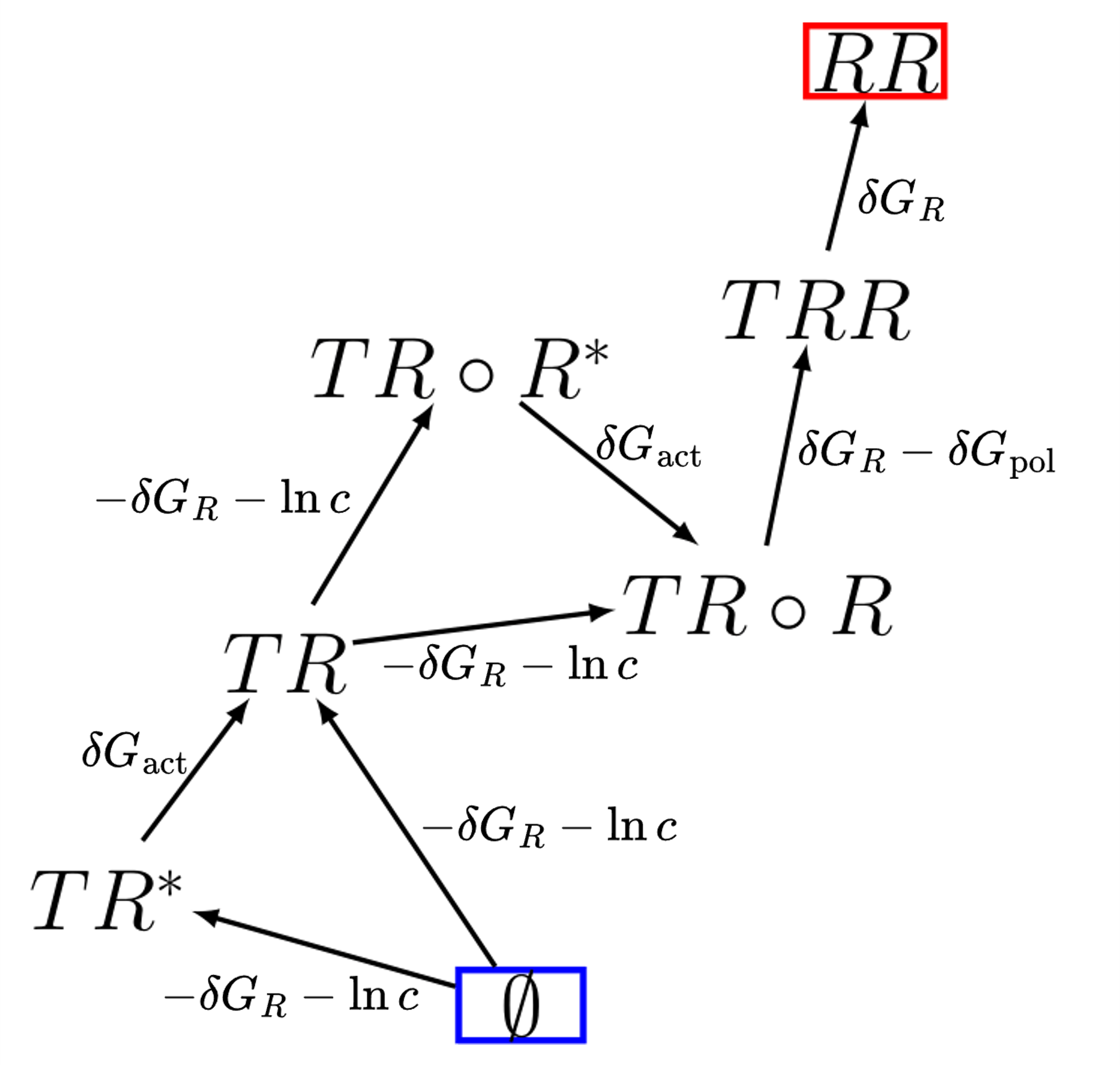
Monomers are now present in inactive (starred) and active forms, with , representing the free-energy change of activation. We assume that each non-activated monomer is chemostatted at the same concentration as each non-activated monomer , . Dropping this assumption would only cause a shift to . As a result, and control the concentration bounds. We assume .
The concentration bounds of this system, determined by the SAWs with maximal and minimal free-energy changes, depend on the values of both the aforementioned free-energy parameters, as well as whether is odd or even. The bounds are set by
| (28) |
and
| (31) |
where the top value in each brace is for even and the bottom value for odd . Unlike the simple system in section V.1, the SAWs that exhibit and are not the intuitively simple pathways that go via the template and the destroyer, respectively. Instead, the extremal pathways correspond to snaking through the CRN, alternately using both the template and destructive catalyst to first create a sequence, and then convert it into another sequence. We show these pathways for in appendix G. These SAWs would not only be absurd as the dominant pathways in a real system, they actually define a bound that is unachievable, even in principle. Since the pathways exhibiting and pass through other products as intermediates, scaling these pathways to be fast would necessarily result in sub-pathways to other products being fast.
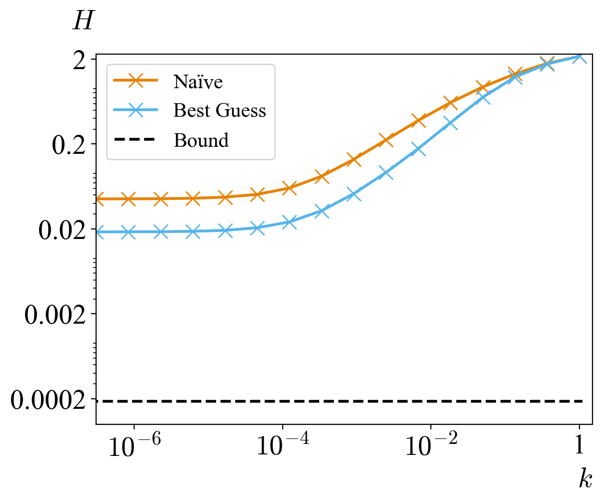
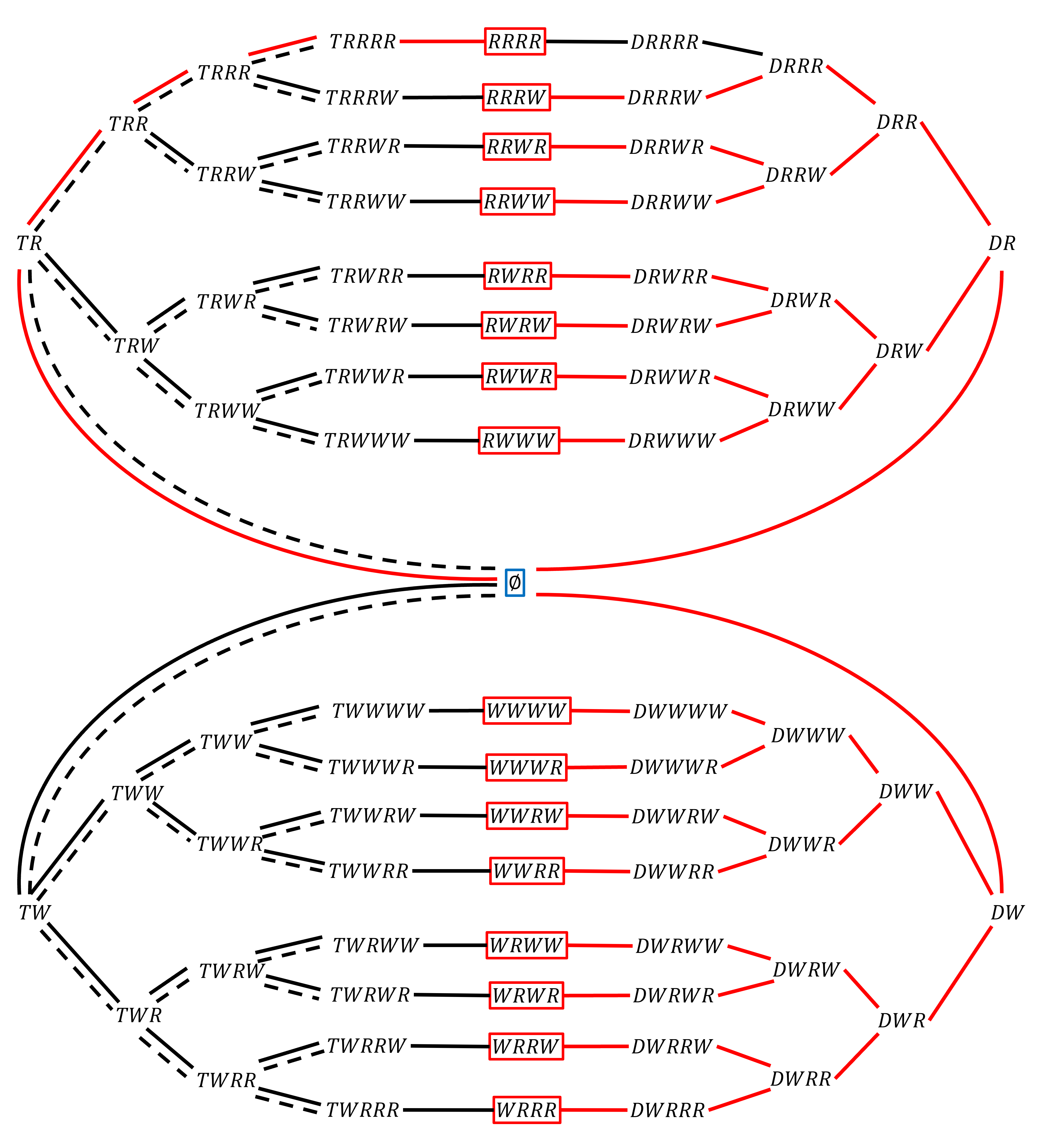
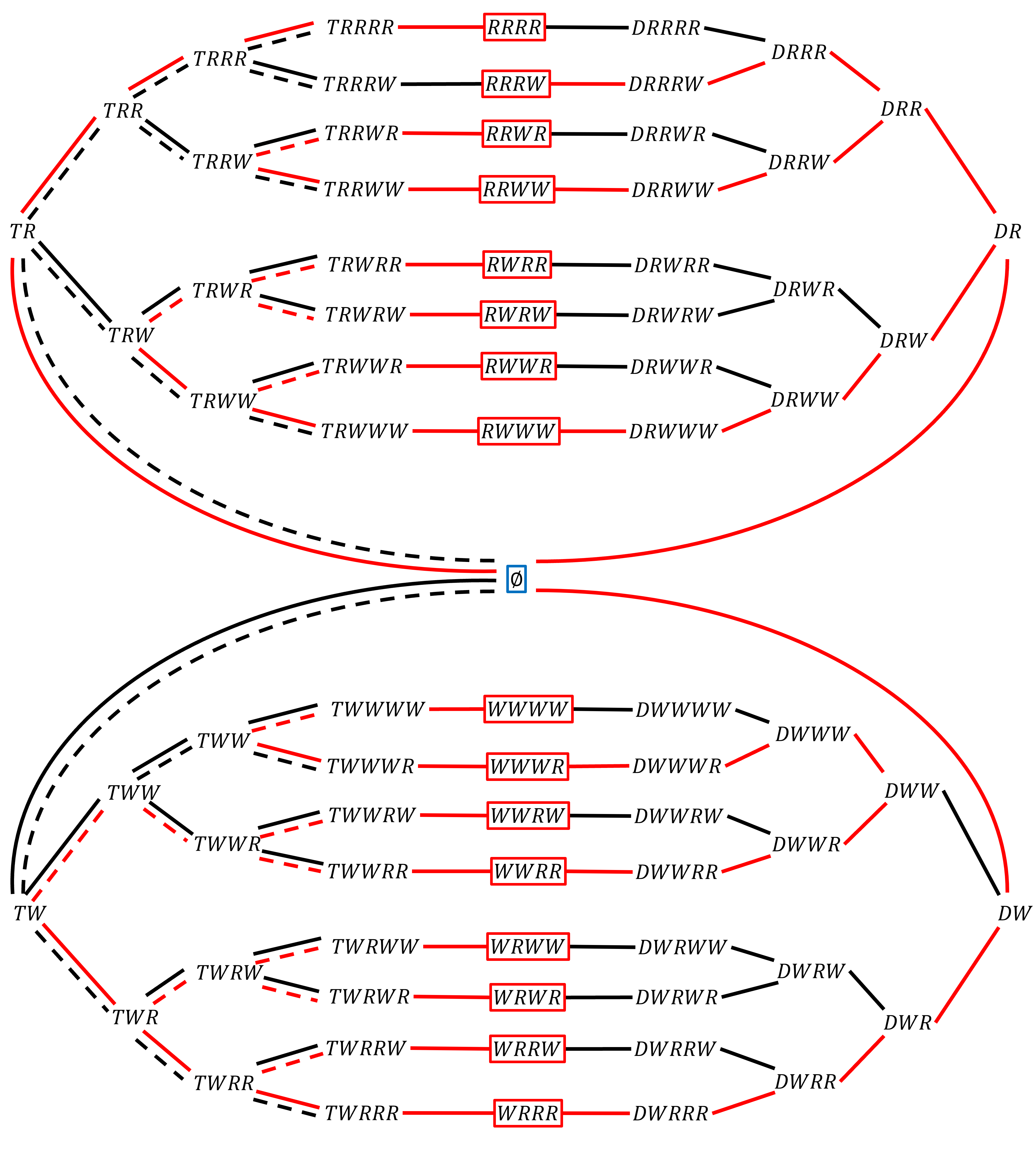
Nonetheless, the existence of these snaking pathways can provide some advantage, at least in principle. In figure 9, we show two attempts to find parameters that minimize entropy for a system with . In the first “naïve” scheme, plotted in blue, reactions contributing to assembly of via the template or assembly of any other sequence via the destructive catalyst are assigned rates of and all other rates are taken as . We show this scheme in appendix G. In the second “best guess” scheme, plotted in red, we make use of these snaking pathways. The reactions contributing to assembly of via the template are still assigned rates of . However, for all other products, the longest snaking pathway which does not intersect with the pathway leading to has rates assigned . Again we show this scheme in more detail in appendix G.
As , the snaking pathways outperform the non-snaking pathways significantly, resulting in approximately half the entropy of the product distribution (figure 9). Notably, however, neither the best guess nor the naïve system converges on the bound as ; the best guess approaches as compared to the bound at two orders of magnitude lower.
Although the the best guess system can outperform the naïve system in principle, when absolute rates can be chosen freely, rates may in practice be mechanistically constrained. As a result, this outperformance may not be achievable in a specific model. Indeed, at moderate , the entropies of the naive system and the best guess converge.
VI Conclusion
Considering systems in which catalysts selectively produce products drawn from a large set of possibilities, we have derived general bounds on the steady-state distribution of products. The maximal difference in free energies between formation paths for the products sets an upper bound on the specificity (or probability with which a single sequence can be selected from the product distribution) and a lower bound on the entropy of that product distribution. These bounds are remarkably simple, applying to arbitrarily complex networks regardless of details such as kinetic proofreading.
Several features of these bounds are, a least to us, unexpected. They modify our understanding that producing sequence-specific products has a “cost” related to the information stored [31, 2, 32], and help to resolve the paradox that thermodynamics imposes limits on templating despite the fact that catalysts can be arbitrarily specific for their substrate with no minimal cost.
Most importantly, the bounds are pseudo-equilibrium in nature. In the optimal system, kinetic selectivity ensures that each product is coupled to only a single pathway, with the yield determined by the equilibrium properties of that pathway. As a result, although maintaining an ensemble with exactly one product drawn from possibilities requires pathways differentiated by , this is not a cost in the sense of entropy production. A low entropy product distribution will be far from equilibrium, with a high non-equilibrium free energy, and will consequently require more chemical work to create it in the first place than a uniform ensemble [2, 29]. But once in the dynamic steady state, a highly-specific ensemble (which is capable of dynamically responding to changing catalyst concentrations) can, in theory, be maintained with negligible “housekeeping” entropy production [45].
Such behaviour is profoundly different from apparently similar information-processing networks, such as a push-pull phosphorylation network [46]. In that case, accurate information transmission is only possible if the system undergoes cyclic phosphorylation by one pathway, and dephosphorylation by another, resulting in a high housekeeping entropy production. Fundamentally, the difference arises because the system considered here relies on catalytic rates distinguishing between different pathways to different products, which is not constrained by entropy production, whereas the push-pull network of [46] relies on catalysts selecting a forwards pathway over its reverse, which is so constrained [33].
Indeed, the thermodynamic limits on the product distribution that do exist do not reflect the actual selectivity of the underlying catalytic processes, which is the typical focus of work on templated processes [7, 8, 9, 10, 11, 12, 13, 14, 15, 26, 27, 16, 17, 25, 6, 18, 19, 20, 21, 22, 29, 30, 28]. The ability of a template to kinetically select certain products determines how close to the bound a system can come, but it does not determine the bound itself. For example, although a single product cannot dominate the steady state for , this does not mean that catalysts cannot be arbitrarily specific; simply that the steady state achieved via the set of available catalysts cannot be dominated by one product. Indeed, remarkably, for the lower bound on product entropy is achieved when a vanishingly small fraction of the possible products dominate the ensemble, even for . Such a distribution could arise from a system with templates each catalysing a single product with high accuracy, and a non-specific destructive catalyst.
The above results suggest that, in some sense, catalytic templating ensembles do not have an inherent minimum maintenance “cost” related to the accuracy of information propagation from a single template to its product. From another perspective, however, our bounds show that maintaining a product distribution that is highly-specific for a single product is hard relative to previous claims [31, 2, 32]. The minimal entropy distribution is only dominated by a single product for , a condition that converges to the more familiar achingly slowly with . Moreover, the minimal entropy of a product distribution with finite is larger than that for for all values of . For any finite , perfect accuracy is only possible in the limit , although good accuracy is possible for .
This work open up several lines of inquiry. Firstly: why do cells not operate in the manner suggested by the optimal behaviour? RNA molecules are not destroyed by the reverse of their creation pathway. As we have noted, the bounds may be formally unachievable even in a system for which rates can be arbitrarily scaled, but even in this context it is theoretically possible to produce sharply-peaked ensembles at low cost via mechanisms that avoid cycling of products via distinct pathways. We expect that practical constraints that would limit the speed and specificity of catalysts operating in this reversible regime must be a factor. It may also be true that, in practical contexts, the “excess” entropy production due to responding to changing conditions [45] dominates of the housekeeping entropy production for the steady state. Indeed, exploring how the behaviour of realistic models that are constrained by the actual chemistry and biological context would be highly informative. We note, however, that synthetic information-processing systems might be engineered to operate in this low-cost fashion - particularly if the products are relatively simple compared to proteins and RNA. Such a system would be reminiscent of the behaviour of dynamic combinatorial chemistry ensembles [47], but with the system designed so that the presence/absence of specific catalysts changes the free energy of the dominant pathway to an assembled product.
Secondly, we have made a number of simplifying assumptions in this work. Most significantly, we have assumed that all products are equally thermodynamically stable, and produced via equivalent pathways. In practice, although the presence of catalysts cannot change the thermodynamic stability of the products, some products will be more stable than others due to intra-product interactions, and network topologies will necessarily vary for polymers of different length. As a result, and will be product-specific in general. In this case, much of our analysis would still apply directly, with individual products pushed either to their maximum or minimum concentration to minimize entropy, and the optimal distribution being achieved when each product is overwhelmingly coupled to a single pathway. However, it will likely be easier to create distributions that are sharply peaked about the most stable products, and harder in other cases. Given that the aim of processes like transcription and translation is to produce functional, rather than stable, products, it is unclear whether this asymmetry would actually be beneficial. It would also be interesting to examine behaviour when either monomers or catalysts are not chemostatted, making the system non-linear.
Finally, we have not considered the dynamics of these networks in detail. We have shown that at finite times, the bounds can be violated, but we have not attempted to explore for how long this is possible. Indeed, one might ask whether cells are effectively in this non-steady-state limit since some theoretically possible polymers (such as chimeric RNA/DNA sequences) are essentially never created by the cell. The question of how these networks respond to dynamical changes in the concentration of the catalysts, and the associated thermodynamic costs, is also open.
Author Contributions
All authors conceived of the project. B.Q. produced the analysis and wrote the initial draft. All authors interpreted results and reviewed and edited this paper.
Data Availability Statement
The Mathematica code that support the findings of this study openly available on Zenodo at https://doi.org/10.5281/zenodo.10909084.
Acknowledgements.
We thank Pieter Rein ten Wolde for his constructive comments on the manuscript. This work is part of a project that has received funding from the European Research Council (ERC) under the European Union’s Horizon 2020 research and innovation program (Grant agreement No. 851910). T.E.O. is supported by a Royal Society University Fellowship.Appendix A Minimizing entropy maximizes channel capacity
We can consider the deterministic CRNs in this paper to be information channels. Let us assume the underlying chemistry, which determines the rate constants appearing in the un-linearized model, and the concentration of monomers, are fixed. The effective rates of the linearized network would then vary with the concentrations of catalysts only. As a specific (simple) example of how the entropy bound defines the channel capacity, let us assume that all variability is due to sequence-specific template catalysts, one for each product, and that of these templates exactly one is present at any given time at a fixed concentration.
We can define the input to the information channel as the template that is present at high concentration; the output would then be a product sampled from the steady state product distribution for that input state. If the templates are symmetric, acting equivalently relative to their ideal sequence, then each output distribution would merely be a permutation of the set of product probabilities.
A system of this kind would define a symmetric channel. The channel capacity of such a symmetric channel [34] is given by in our notation, where is the number of products/sequence-specific templates, and the Shannon entropy of the output distribution for any single template. This entropy will be the same for any input state in our symmetrized description. Hence, minimizing the entropy maximizes the channel capacity.
Appendix B Proof of the steady state concentration written as sum over spanning trees
We note that a similar result can be seen in e.g. [39]. However, we prove this result here with particular reference to the effect of a null species.
Consider a linear connected CRN under mass action kinetics. Let be the chemical species with concentration . Assume the CRN contains some reactions of the form . Without loss of generality, we assume that there only exists at most one reaction of the form (for the cases where there are multiple such reactions, replace their reaction rate with the sum over all reaction rates of reactions of that form). We may cast the steady state equation for the vector of steady state concentrations of the chemical species, , as the linear equation:
| (32) |
where is a vector such that entry is the reaction rate of the reaction , and is a matrix with off diagonal entries equal to the reaction rate of the reaction and diagonal elements equal to minus the sum of reaction rates of reactions over all chemical species as well as . Note that the sum of column of matrix is equal to minus the reaction rate of reaction . Thus, we may create the new matrix:
| (37) |
where is a vector such that entry is equal to the reaction rate of reaction . The columns of the matrix, , now sum to zero and we can use the all minors matrix tree theorem [48]. Represent as a graph with nodes corresponding to chemical species and an additional node corresponding to , and edges corresponding to reactions between species with weights equal to their reaction rate constants . Then, the determinant (up to a sign) of the sub matrix formed by deleting row and column from matrix is given by the sum over the set of spanning trees rooted at node , ,
| (38) |
where represents matrix with row and column deleted. In particular,
| (39) |
Thus, by Cramers rule [49], and the sign of the determinant under swapping of rows, eq. 2 gives the solution to eq. 32.
Appendix C Proof of boundedness of steady-state concentrations
We note that similar proofs exist in the literature [41, 42, 39, 40], but we have included the proof here for completeness and to match our specific conventions. Further, in the cases considered in this paper, the fact that all products are connected to the null state means that our result bounds the absolute, rather than a relative, concentrations.
Consider a linear connected CRN with chemical species and some reactions of the form . The concentration of species may be written as in eq 2. The numerator and denominator in this fraction are sums over spanning trees rooted at a given node. A sum over spanning trees rooted at node may be factored into a sum over self avoiding walks (SAWs) from some arbitrary other node to node . Concretely, letting be the other, arbitrary node, and be the set of SAWs from to ,
| (40) |
where is a factor that, crucially, is the same for the equivalent (reversed) SAW in , in which all edges are reversed compared to . That is to say, if we now wish to find the sum over spanning trees rooted at , we may choose as the arbitrary other state and find:
| (41) |
where is the reverse of edge . For the linear CRNs, utilising eq 3, we may thus write:
| (42) | |||||
Hence,
| (43) |
as required.
Appendix D Proof of the boundedness of steady-state distribution entropy
We have a set of concentrations . Denote the total concentration . From these concentrations we can define a distribution where . The Shannon entropy of this distribution is
| (44) |
Suppose that each concentration is bounded by the same upper and lower bounds, . We now propose that the distribution of concentrations that minimises the entropy, , is that with of the species at concentration and at concentration , where is either
| (45) |
To prove this claim, let us calculate the derivative of with respect to a concentration , holding all other concentrations fixed and remembering that is linear in ,
| (46) |
Additionally, we require the second derivative,
| (47) |
Evaluating the second derivative at , the first two terms are zero and the third is necessarily negative for non-zero . Thus
| (48) |
And so, for any distribution, we can decrease the by increasing the concentrations of any species for which and decreasing the concentrations for any species whose concentration has . For species for which , changing the concentration in either direction will decrease . Consequently, minimising the entropy of the distribution necessarily requires all species to be at one bound or the other: we need species at concentration and at concentration . Hence, we have transformed the problem into a one dimensional one of minimising as a function of . We can write this entropy as
| (49) |
Taking the derivative with respect to and setting it to zero tells us that
| (50) |
gives a turning point for , which is clearly a minimum since is maximal entropy. Since has only a single turning point as a function of , the integer that minimises will be either the floor or ceiling of the above expression, and is given by eqs. 12 and 13.
Appendix E Chemical reaction network for example 1
We present here the full chemical reaction network used for section V.1.
for , . Dynamics is assumed to follow mass action kinetics, with rate constants given above and below the harpoons. represents the template, the destructive catalyst and the “right” and “wrong” monomers. The products are , representing the polymers of length . Here, there are different products. and represent partial polymers, , bound to the template or destructive catalyst. Monomer binds to the template or destructive catalyst with standard free-energy and the standard free-energy of polymerisation is in the absence of fuel. The destructive catalyst has an additional free energy per length driving the disassembly of polymers.
Let us consider a set of rate constants that allow us to saturate (in a certain limit) the bound for specificity maximisation. We may for example, set the rates of , , …, , equal to a non-zero constant (here, corresponds to copies of ). We also set all the rates of , , …, , , where or but excluding all being , equal to 1. Conversely, we set the rates of , , …, , and , , …, , , where or but excluding all being , equal to . The reverse reactions of those listed above have a rate determined by the free-energy change of reaction. For , this set of reaction rates saturates the bound.
Appendix F Chemical reaction network for example 2
Similarly, we present the full CRN used for section V.2.
where , . As in the previous CRN, represents the template, the destructive catalyst, the “right” monomers and the “wrong” monomers. and are non-activated monomers. Dynamics is assumed to follow mass action kinetics, with rate constants given above and below the harpoons. The species, () represent a complex of polymer of length bound to the template as well as a (non-)activated monomer () bound, but not yet polymerised into a single polymer of length . are the products. Both non-activated () and activated monomers () bind to the template or destructive catalyst with standard free energy . If an non-activated monomer is bound to the template, it may be activated, with a free-energy change . If an activated monomer is bound to the template, it may be polymerised into the growing copolymer; the standard free-energy change of polymerisation is . The destructive catalyst has an additional free-energy per length driving the disassembly of polymers.
Appendix G Pathways for example 2
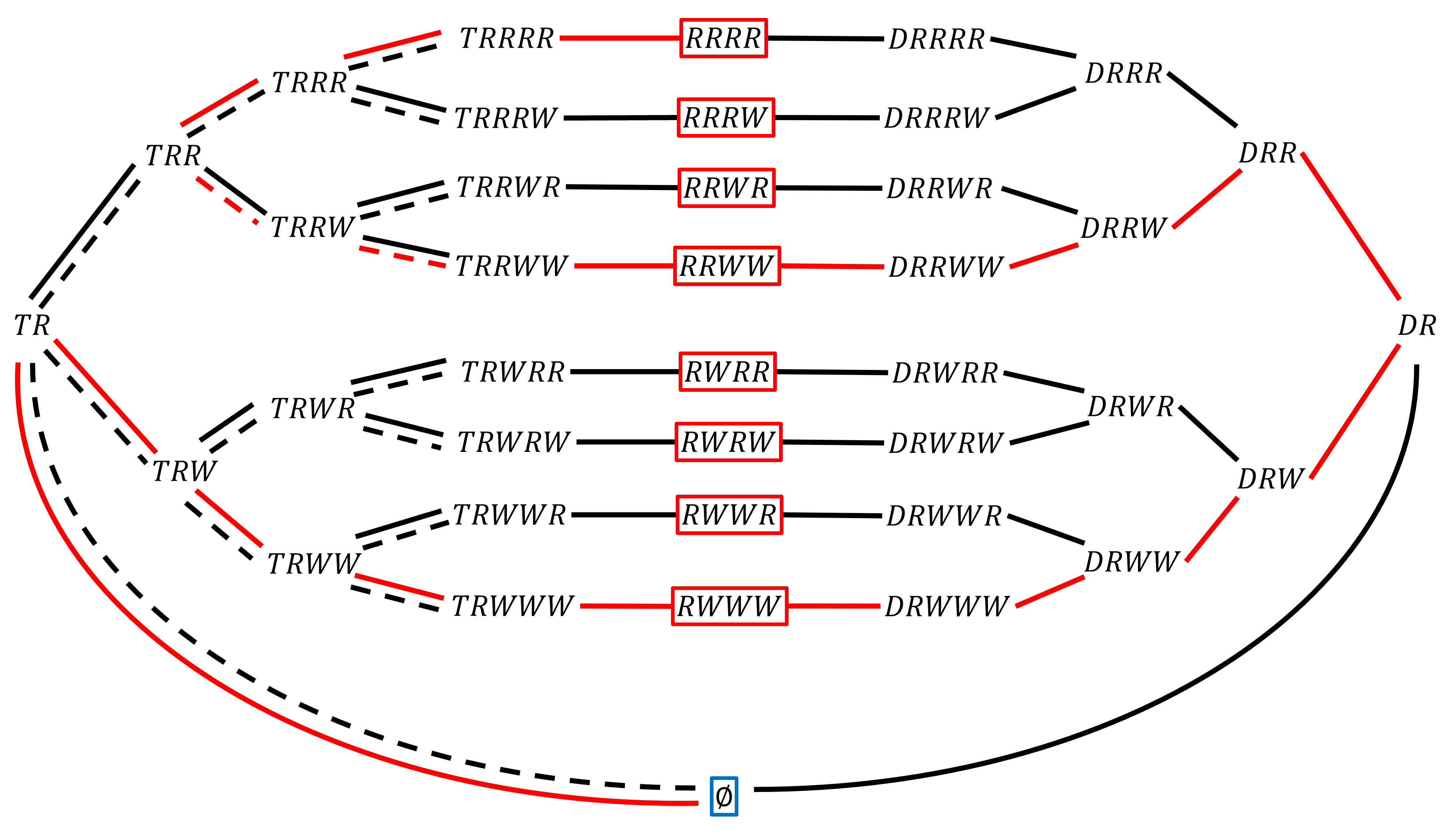
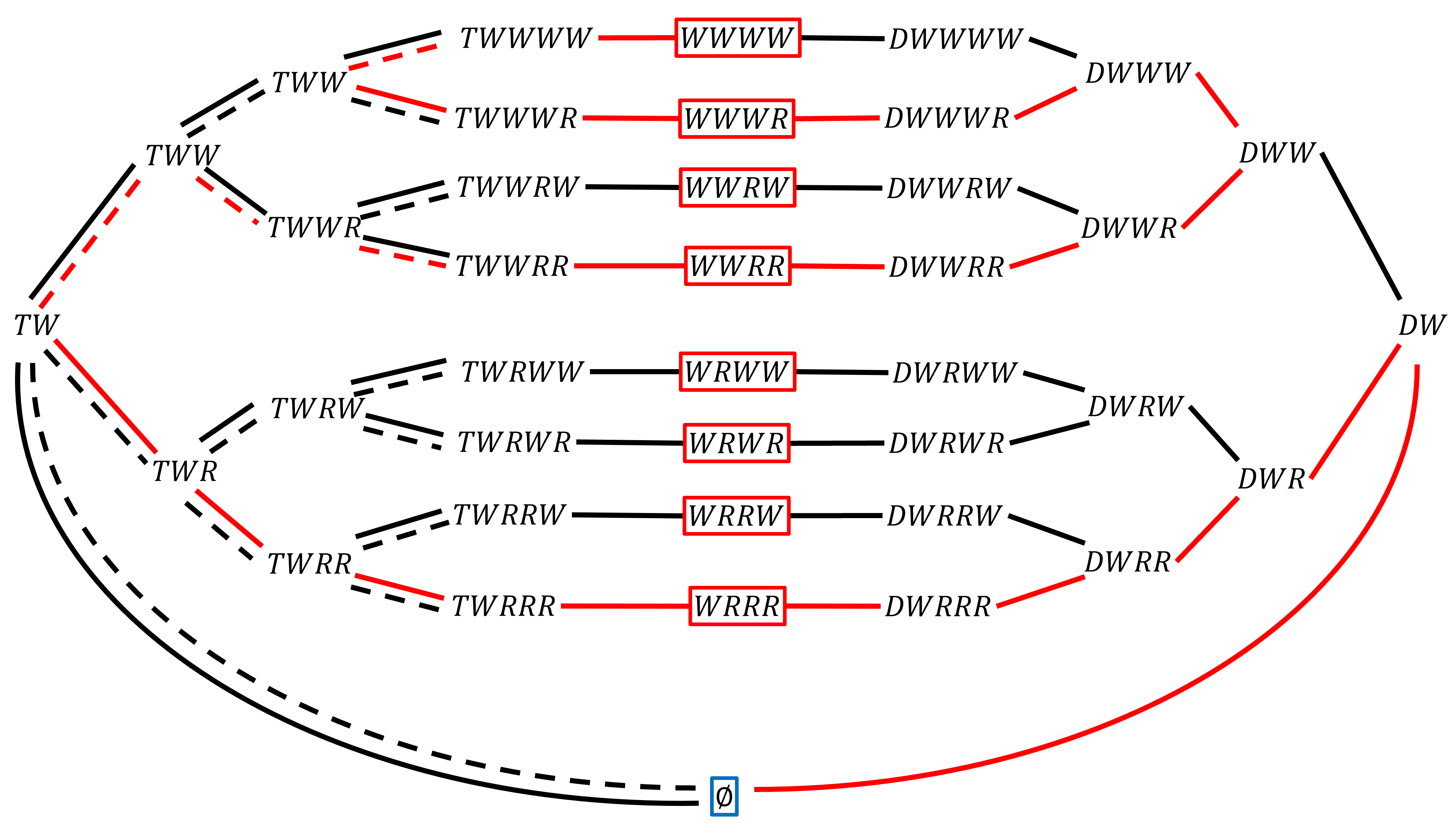
In this appendix, for the kinetic proofreading CRN (section V.2) we depict the pathways of most positive/negative free-energy change (figure 10) as well as the fast reactions used for the two attempts to minimize the entropy, the naïve attempt (figure 11) and our best guess (figure 12). For simplicity, we have coarse-grained the intermediate states for the reactions involving templates, and have presented these processes using two lines for the pathways through the kinetic proofreading motifs. The solid line represents the inactivated monomer pathway ( ) and the dashed line represents the active monomer pathway (). Extremal pathways (figure 10) and fast reactions with rates (figure 11 and figure 12) are highlighted in red.
References
- Crick [1970] F. Crick, Central dogma of molecular biology, Nature 227, 561 (1970).
- Ouldridge and ten Wolde [2017] T. E. Ouldridge and P. R. ten Wolde, Fundamental costs in the production and destruction of persistent polymer copies, Physical Review Letters 118, 158103 (2017).
- Watson [2014] J. D. Watson, Molecular biology of the gene, seventh edition. ed. (Benjamin-Cummings Publishing Company, Boston, 2014).
- Hopfield [1974] J. J. Hopfield, Kinetic proofreading: a new mechanism for reducing errors in biosynthetic processes requiring high specificity, Proceedings of the National Academy of Sciences of the United States of America 71, 4135 (1974).
- Ninio [1975] J. Ninio, Kinetic amplification of enzyme discrimination, Biochimie 57, 587 (1975).
- Bennett [1979] C. H. Bennett, Dissipation-error tradeoff in proofreading, BioSystems 11, 85 (1979).
- Murugan et al. [2014] A. Murugan, D. A. Huse, and S. Leibler, Discriminatory proofreading regimes in nonequilibrium systems, Physical Review X 4, 021016 (2014).
- Murugan et al. [2012] A. Murugan, D. A. Huse, and S. Leibler, Speed, dissipation, and error in kinetic proofreading, Proceedings of the National Academy of Sciences of the United States of America 109, 12034 (2012).
- Yu et al. [2022] Q. Yu, A. B. Kolomeisky, and O. A. Igoshin, The energy cost and optimal design of networks for biological discrimination, Journal of the Royal Society Interface 19, 20210883 (2022).
- Sahoo and Klumpp [2013] M. Sahoo and S. Klumpp, Backtracking dynamics of rna polymerase: pausing and error correction, Journal of Physics: Condensed Matter 25, 374104 (2013).
- Sahoo et al. [2021] M. Sahoo, N. Arsha, P. R. Baral, and S. Klumpp, Accuracy and speed of elongation in a minimal model of dna replication, Physical Review E 104, 034417 (2021).
- Ehrenberg and Blomberg [1980] M. Ehrenberg and C. Blomberg, Thermodynamic constraints on kinetic proofreading in biosynthetic pathways, Biophysical Journal 31, 333 (1980).
- Song et al. [2016] Y.-S. Song, Y.-G. Shu, X. Zhou, Z.-C. Ou-Yang, and M. Li, Proofreading of dna polymerase: a new kinetic model with higher-order terminal effects, Journal of Physics: Condensed Matter 29, 025101 (2016).
- Song and Hyeon [2020] Y. Song and C. Hyeon, Thermodynamic cost, speed, fluctuations, and error reduction of biological copy machines, The Journal of Physical Chemistry Letters 11, 3136 (2020).
- Li et al. [2019] Q.-S. Li, P.-D. Zheng, Y.-G. Shu, Z.-C. Ou-Yang, and M. Li, Template-specific fidelity of dna replication with high-order neighbor effects: A first-passage approach, Physical Review E 100, 012131 (2019).
- Wong et al. [2018] F. Wong, A. Amir, and J. Gunawardena, Energy-speed-accuracy relation in complex networks for biological discrimination, Physical Review E 98, 012420 (2018).
- Piñeros and Tlusty [2020] W. D. Piñeros and T. Tlusty, Kinetic proofreading and the limits of thermodynamic uncertainty, Physical Review E 101, 022415 (2020).
- Nguyen and Vaikuntanathan [2016] M. Nguyen and S. Vaikuntanathan, Design principles for nonequilibrium self-assembly, Proceedings of the National Academy of Sciences of the United States of America 113, 14231 (2016).
- Galstyan and Phillips [2019] V. Galstyan and R. Phillips, Allostery and kinetic proofreading, The Journal of Physical Chemistry B 123, 10990 (2019).
- Rao and Peliti [2015] R. Rao and L. Peliti, Thermodynamics of accuracy in kinetic proofreading: dissipation and efficiency trade-offs, Journal of Statistical Mechanics: Theory and Experiment 2015, P06001 (2015).
- Banerjee et al. [2017] K. Banerjee, A. B. Kolomeisky, and O. A. Igoshin, Elucidating interplay of speed and accuracy in biological error correction, Proceedings of the National Academy of Sciences of the United States of America 114, 5183 (2017).
- Chiuchiù et al. [2019] D. Chiuchiù, Y. Tu, and S. Pigolotti, Error-speed correlations in biopolymer synthesis, Physical Review Letters 123, 038101 (2019).
- Sartori and Pigolotti [2013] P. Sartori and S. Pigolotti, Kinetic versus energetic discrimination in biological copying, Physical Review Letters 110, 188101 (2013).
- Gaspard and Andrieux [2014] P. Gaspard and D. Andrieux, Kinetics and thermodynamics of first-order markov chain copolymerization, The Journal of Chemical Physics 141, 044908 (2014).
- Poulton et al. [2019] J. M. Poulton, P. R. Ten Wolde, and T. E. Ouldridge, Nonequilibrium correlations in minimal dynamical models of polymer copying, Proceedings of the National Academy of Sciences 116, 1946 (2019).
- Pigolotti and Sartori [2016] S. Pigolotti and P. Sartori, Protocols for copying and proofreading in template-assisted polymerization, Journal of Statistical Physics 162, 1167 (2016).
- Sartori and Pigolotti [2015] P. Sartori and S. Pigolotti, Thermodynamics of error correction, Physical Review X 5, 041039 (2015).
- Qureshi et al. [2023] B. Qureshi, J. Juritz, J. M. Poulton, A. Beersing-Vasquez, and T. E. Ouldridge, A universal method for analyzing copolymer growth, The Journal of Chemical Physics 158, 104906 (2023).
- Poulton and Ouldridge [2021] J. M. Poulton and T. E. Ouldridge, Edge-effects dominate copying thermodynamics for finite-length molecular oligomers, New Journal of Physics 23, 063061 (2021).
- Juritz et al. [2022] J. Juritz, J. M. Poulton, and T. E. Ouldridge, Minimal mechanism for cyclic templating of length-controlled copolymers under isothermal conditions, The Journal of Chemical Physics 156, 074103 (2022).
- Bennett [1982] C. H. Bennett, The thermodynamics of computation—a review, International Journal of Theoretical Physics 21, 905 (1982).
- Genthon et al. [2024] A. Genthon, C. D. Modes, F. Jülicher, and S. W. Grill, Non equilibrium transitions in a polymer replication ensemble, arXiv preprint arXiv:2403.05665 (2024).
- Ouldridge [2018] T. E. Ouldridge, The importance of thermodynamics for molecular systems, and the importance of molecular systems for thermodynamics, Natural Computing 17, 3 (2018).
- Cover and Thomas [2006] T. M. Cover and J. A. Thomas, Elements of information theory, second edition. ed. (Wiley-Interscience, Hoboken, N.J, 2006).
- Shannon [1948] C. E. Shannon, A mathematical theory of communication, The Bell system technical journal 27, 379 (1948).
- Polettini and Esposito [2014] M. Polettini and M. Esposito, Irreversible thermodynamics of open chemical networks. i. emergent cycles and broken conservation laws, The Journal of Chemical Physics 141, 024117 (2014).
- Rao and Esposito [2016] R. Rao and M. Esposito, Nonequilibrium thermodynamics of chemical reaction networks: Wisdom from stochastic thermodynamics, Phys. Rev. X 6, 041064 (2016).
- Anderson et al. [2010] D. F. Anderson, G. Craciun, and T. G. Kurtz, Product-form stationary distributions for deficiency zero chemical reaction networks, Bulletin of Mathematical Biology 72, 1947 (2010).
- Nam et al. [2022] K.-M. Nam, R. Martinez-Corral, and J. Gunawardena, The linear framework: using graph theory to reveal the algebra and thermodynamics of biomolecular systems, Interface Focus 12, 20220013 (2022).
- Çetiner and Gunawardena [2022] U. Çetiner and J. Gunawardena, Reformulating nonequilibrium steady states and generalized hopfield discrimination, Physical Review E 106, 064128 (2022).
- Maes and Netočnỳ [2013] C. Maes and K. Netočnỳ, Heat bounds and the blowtorch theorem, in Annales Henri Poincaré, Vol. 14 (Springer, 2013) pp. 1193–1202.
- Sáez et al. [2019] M. Sáez, E. Feliu, and C. Wiuf, Linear elimination in chemical reaction networks, in Recent Advances in Differential Equations and Applications (Springer International Publishing, Cham, 2019) pp. 177–193.
- Nelson [2020] P. C. Nelson, Biological physics: energy, information, life (Chiliagon Science, Philadelphia PA USA, 2020).
- Mallory et al. [2020] J. D. Mallory, O. A. Igoshin, and A. B. Kolomeisky, Do we understand the mechanisms used by biological systems to correct their errors?, The Journal of Physical Chemistry B 124, 9289 (2020).
- Seifert [2012] U. Seifert, Stochastic thermodynamics, fluctuation theorems and molecular machines, Reports on progress in physics 75, 126001 (2012).
- Ouldridge et al. [2017] T. E. Ouldridge, C. C. Govern, and P. R. ten Wolde, Thermodynamics of computational copying in biochemical systems, Phys. Rev. X 7, 021004 (2017).
- Ladame [2008] S. Ladame, Dynamic combinatorial chemistry: on the road to fulfilling the promise, Org. Biomol. Chem. 6, 219 (2008).
- Chaiken [1982] S. Chaiken, A combinatorial proof of the all minors matrix tree theorem, SIAM Journal on Algebraic Discrete Methods 3, 319 (1982).
- Robinson [1970] S. M. Robinson, A short proof of cramer’s rule, Mathematics Magazine 43, 94 (1970).